On the convergence of Jacobi-type algorithms for Independent Component Analysis

Abstract

Jacobi-type algorithms for simultaneous approximate diagonalization of real (or complex) symmetric tensors have been widely used in independent component analysis (ICA) because of their good performance. One natural way of choosing the index pairs in Jacobi-type algorithms is the classical cyclic ordering, while the other way is based on the Riemannian gradient in each iteration. In this paper, we mainly review in an accessible manner our recent results in a series of papers about weak and global convergence of these Jacobi-type algorithms. These results are mainly based on the Lojasiewicz gradient inequality.

I Introduction

Let $\mathcal{M}$ be the orthogonal group $\mathscr{O}_{n}$ or the unitary group $\mathscr{U}_{n}$. In this paper, we mainly study the following problem, which is to maximize a smooth function

$$\textit{f}:\mathcal{M}\to\mathbb{R}.$$ (1)

The cost functions in Example I.1 and Example I.2 are all in the form of problem (1), and they are important in blind source separation and Independent Component Analysis (ICA) [1, 2, 3, 4].

Let $\mathbb{F}=\mathbb{R}$ or $\mathbb{C}$. Let $\mathbb{F}^{n_{1}\times\cdots\times n_{d}}\stackrel{{\scriptstyle\sf def}}{{=}}\mathbb{F}^{n_{1}}\otimes\cdots\otimes\mathbb{F}^{n_{d}}$ be the linear space of $d$-th order tensors [5, 6, 7, 8, 9]. For $\boldsymbol{\mathcal{W}}\in\mathbb{F}^{n\times\cdots\times n}$, we denote by $\mathop{\operator@font diag}\{\boldsymbol{\mathcal{W}}\}$ the vector of its diagonal elements, and $\mathop{\operator@font tr}\{\boldsymbol{\mathcal{W}}\}$ the trace function. We denote by $\|\cdot\|$ the Frobenius norm of a tensor or a matrix, or the Euclidean norm of a vector. Operator $\mathop{\bullet_{p}}$ denotes contraction on the $p$-th index of a tensor; when contracted with a matrix, it is understood that summation is always performed on the second index of the matrix. For instance, $(\boldsymbol{\mathcal{A}}\mathop{\bullet_{1}}\boldsymbol{M})_{ijk}=\sum_{\ell}\mathcal{A}_{\ell jk}M_{i\ell}$.

Example I.1 ([10, Section 1]).

Let $\{\boldsymbol{\mathcal{A}}^{(\ell)}\}_{1\leq\ell\leq L}\subseteq\mathbb{R}^{n\times\cdots\times n}$ be a set of $d$-th order real symmetric tensors [11]. The simultaneous approximate diagonalization of symmetric tensors problem is to maximize

$$f(\boldsymbol{Q})=\sum_{\ell=1}^{L}\|\mathop{\operator@font diag}\{\boldsymbol{\mathcal{A}}^{(\ell)}\mathop{\bullet_{1}}\boldsymbol{Q}^{{\sf T}}\cdots\mathop{\bullet_{d}}\boldsymbol{Q}^{{\sf T}}\}\|^{2},$$ (2)

where $\boldsymbol{Q}\in\mathscr{O}_{n}$. This problem includes the following well-known problems in ICA as special cases:
(i) approximate tensor diagonalization problem [12, 2, 13, 14], if $L=1$ and $d>2$;
(ii) simultaneous approximate matrix diagonalization problem [15], if $L>1$ and $d=2$.

Example I.2 ([16, Section 2]).

Let $\boldsymbol{\mathcal{A}}^{(\ell)}\in\mathbb{C}^{n\times\cdots\times n}$ be a $d_{\ell}$-th order complex tensor for $1\leq\ell\leq L$ (orders $d_{1},\ldots,d_{L}$ are potentially different). For integers $t_{\ell}$ satisfying $0\leq t_{\ell}\leq d_{\ell}$ and $\alpha_{\ell}\in\mathbb{R}$ (possibly negative), the cost function is defined as

$$f(\boldsymbol{U}) =\sum\limits_{\ell=1}^{L}\alpha_{\ell}\|\mathop{\operator@font diag}\{\boldsymbol{\mathcal{W}}^{(\ell)}\}\|^{2},\ \ \textrm{where}$$ (3)

$$\boldsymbol{\mathcal{W}}^{(\ell)} =\boldsymbol{\mathcal{A}}^{(\ell)}\mathop{\bullet_{1}}\boldsymbol{U}^{{\sf H}}\cdots\mathop{\bullet_{t_{\ell}}}\boldsymbol{U}^{{\sf H}}\mathop{\bullet_{t_{\ell}+1}}\boldsymbol{U}^{{\sf T}}\cdots\mathop{\bullet_{d_{\ell}}}\boldsymbol{U}^{{\sf T}}.$$

Let $d=\max(d_{1},\ldots,d_{L})$. It can be shown that $f$ admits representation (3) if and only if there exists a $2d$-th order Hermitian[18] complex tensor $\boldsymbol{\mathcal{B}}$, such that $f$ has a representation

$$f(\boldsymbol{U}) =\mathop{\operator@font tr}\{\boldsymbol{\mathcal{V}}\},\ \ \textrm{where}$$ (4)

$$\boldsymbol{\mathcal{V}} =\boldsymbol{\mathcal{B}}\mathop{\bullet_{1}}\boldsymbol{U}^{{\sf H}}\cdots\mathop{\bullet_{d}}\boldsymbol{U}^{{\sf H}}\mathop{\bullet_{d+1}}\boldsymbol{U}^{{\sf T}}\cdots\mathop{\bullet_{2d}}\boldsymbol{U}^{{\sf T}}.$$

This cost function includes the following well-known problems in ICA as special cases:
(i) simultaneous approximate Hermitian diagonalization of complex matrices [19]. Let $\boldsymbol{A}^{(\ell)}\in\mathbb{C}^{n\times n}$. The cost function is defined as

$$f(\boldsymbol{U})=\sum\limits_{\ell=1}^{L}\|\mathop{\operator@font diag}\{\boldsymbol{U}^{{\sf H}}\boldsymbol{A}^{(\ell)}\boldsymbol{U}\}\|^{2}.$$ (5)

(ii) approximate diagonalization of a 3rd order complex tensor [3, 4]. Let $\boldsymbol{\mathcal{A}}\in\mathbb{C}^{n\times n\times n}$. The cost function is defined as

$$f(\boldsymbol{U})=\|\mathop{\operator@font diag}\{\boldsymbol{\mathcal{A}}\mathop{\bullet_{1}}\boldsymbol{U}^{{\sf H}}\mathop{\bullet_{2}}\boldsymbol{U}^{{\sf T}}\mathop{\bullet_{3}}\boldsymbol{U}^{{\sf T}}\}\|^{2}.$$ (6)

(iii) approximate diagonalization of a 4th order complex tensor [20]. Let $\boldsymbol{\mathcal{B}}\in\mathbb{C}^{n\times n\times n\times n}$ be Hermitian. The cost function is defined as

$$f(\boldsymbol{U})=\mathop{\operator@font tr}\{\boldsymbol{\mathcal{B}}\mathop{\bullet_{1}}\boldsymbol{U}^{{\sf H}}\mathop{\bullet_{2}}\boldsymbol{U}^{{\sf H}}\mathop{\bullet_{3}}\boldsymbol{U}^{{\sf T}}\mathop{\bullet_{4}}\boldsymbol{U}^{{\sf T}}\}.$$ (7)

To solve problem (1), Jacobi-like sweeping procedure is a popular method, which can break a high-dimensional optimization problem into a sequence of one or two dimensional subproblems. This method often has a very high speed, as the solution of the subproblem can often be written in closed form. In particular, there have been several Jacobi-type algorithms proposed for the cost functions (2) and (3) in ICA, e.g., the well-known Jacobi CoM2 algorithm [1, 2, 12, 4] and Joint approximate diagonalization of eigenmatrices (JADE) algorithm [15, 19].

In this paper, we mainly review our recent results [10, 21, 16, 22] about the weak convergence and global convergence of Jacobi-type algorithms on $\mathcal{M}$. In Section II, we introduce the general Jacobi algorithm on $\mathcal{M}$, as well as the Jacobi-C algorithms. In Section III, we introduce the Jacobi-G algorithms, and present our convergence results about them. Section IV includes some experiments.

II Jacobi-type algorithms

II-A General Jacobi algorithm on $\mathscr{O}_{n}$

Let $\theta\in\mathbb{R}$ be an angle and $(i,j)$ be a pair of indices with $1\leq i<j\leq n$. Denote by $\boldsymbol{G}^{(i,j,\theta)}$ the Givens rotation matrix, as defined e.g., in [23, 4, 10]. The general Jacobi algorithm for problem (1) on $\mathscr{O}_{n}$ can be summarized as in Algorithm 1. In this algorithm, if several equivalent maximizers are present in (8), we choose the one with the angle of smallest magnitude.

Algorithm 1 General Jacobi algorithm on $\mathscr{O}_{n}$

1:  Input: a starting point $\boldsymbol{Q}_{0}$

2:  Output: sequence of iterates $\boldsymbol{Q}_{k}$

3:  for  $k=1,2,\ldots$ do

4:     Choose the pair $(i_{k},j_{k})$ according to a certain pair selection rule

5:     Compute $\theta^{*}_{k}$ that maximizes

$$h_{k}(\theta)\stackrel{{\scriptstyle\sf def}}{{=}}{f}(\boldsymbol{Q}_{k-1}\boldsymbol{G}^{(i_{k},j_{k},\theta)})$$ (8)

6:     Update $\boldsymbol{Q}_{k}=\boldsymbol{Q}_{k-1}\boldsymbol{G}^{(i_{k},j_{k},\theta^{*}_{k})}$

7:  end for

II-B General Jacobi algorithm on $\mathscr{U}_{n}$

Let $\boldsymbol{\Psi}\in\mathscr{U}_{2}$. Denote by $\boldsymbol{G}^{(i,j,\boldsymbol{\Psi})}$ the plane transformation matrix, as defined e.g., in [16, 4]. The general Jacobi algorithm for problem (1) on $\mathscr{U}_{n}$ can be summarized as in Algorithm 2.

Algorithm 2 General Jacobi algorithm on $\mathscr{U}_{n}$

1:  Input: a starting point $\boldsymbol{U}_{0}$

2:  Output: sequence of iterates $\boldsymbol{U}_{k}$

3:  for $k=1,2,\ldots$ do

4:     Choose the pair $(i_{k},j_{k})$ according to a certain pair selection rule

5:     Compute $\boldsymbol{\Psi}_{k}^{*}$ that maximizes

$$h_{k}(\boldsymbol{\Psi})\stackrel{{\scriptstyle\sf def}}{{=}}f(\boldsymbol{U}_{k-1}\boldsymbol{G}^{(i_{k},j_{k},\boldsymbol{\Psi})})$$ (9)

6:     Update $\boldsymbol{U}_{k}=\boldsymbol{U}_{k-1}\boldsymbol{G}^{(i_{k},j_{k},\boldsymbol{\Psi}_{k}^{*})}$

7:  end for

II-C Jacobi-C algorithms

One natural pair selection rule in Algorithm 1 and Algorithm 2 is in cyclic fashion [23, 4] as follows:

$${\small\begin{split}&(1,2)\to(1,3)\to\cdots\to(1,n)\to\\ &(2,3)\to\cdots\to(2,n)\to\\ &\cdots\to(n-1,n)\to\\ &(1,2)\to(1,3)\to\cdots.\end{split}}$$ (10)

The Jacobi algorithm with cyclic rule (10) is called Jacobi-C algorithm. Although this cyclic rule is very simple, the convergence of Jacobi-C algorithms is difficult to study. In [21, Remark 6.5], we proved that, if $f$ is the cost function in (2) with $d=3$ and $L=1$, then Jacobi-C algorithm may converge to a saddle point of $f$. To our knowledge, the convergence of Jacobi-C algorithms for cost functions (2) and (3) is still unknown, except in the single matrix case [23].

III Convergence analysis of Jacobi-G algorithms

In this section, we mainly present our recent results [10, 16, 22] about weak and global convergence of Algorithm 1 and Algorithm 2 under a gradient based pair selection rule. Before that, we need to first recall the well-known Łojasiewicz gradient inequality[24, 25, 26, 27].

III-A Łojasiewicz gradient inequality

Let ${T}_{\boldsymbol{x}}\mathcal{M}$ be the tangent space at $\boldsymbol{x}$. Let $\nabla\textit{f}(\boldsymbol{x})$ be the Euclidean gradient, and $\mathop{{\operator@font grad}}f(\boldsymbol{x})$ be the projection of $\nabla\textit{f}(\boldsymbol{x})$ on ${T}_{\boldsymbol{x}}\mathcal{M}$, i.e., the Riemannian gradient [28]. The following results were proved in [26].

Lemma III.1.

Let $\mathcal{M}\subseteq\mathbb{R}^{n}$ be an analytic submanifold. Then any point $\boldsymbol{x}\in\mathcal{M}$ satisfies a Łojasiewicz inequality for $\mathop{{\operator@font grad}}f(\cdot)$, that is, there exist $\delta>0$, $\sigma>0$ and $\zeta\in(0,1/2]$ such that for all $\boldsymbol{y}\in\mathcal{M}$ with $\|\boldsymbol{y}-\boldsymbol{x}\|<\delta$, it holds that

$$|\textit{f}(\boldsymbol{y})-\textit{f}(\boldsymbol{x})|^{1-\zeta}\leq\sigma\|\mathop{{\operator@font grad}}f(\boldsymbol{y})\|.$$ (11)

Theorem III.2 ([26, Theorem 2.3]).

Let $\mathcal{M}\subseteq\mathbb{R}^{n}$ be an analytic submanifold and $\{\boldsymbol{x}_{k}\}_{k\geq 1}\subseteq\mathcal{M}$ be a sequence. Suppose that $f$ is real analytic and, for large enough $k$,
(i) there exists $\sigma>0$ such that

$$|\textit{f}(\boldsymbol{x}_{k+1})-\textit{f}(\boldsymbol{x}_{k})|\geq\sigma\|\mathop{{\operator@font grad}}f(\boldsymbol{x}_{k})\|\|\boldsymbol{x}_{k+1}-\boldsymbol{x}_{k}\|;$$

(ii) $\mathop{{\operator@font grad}}f(\boldsymbol{x}_{k})=0$ implies that $\boldsymbol{x}_{k+1}=\boldsymbol{x}_{k}$.
Then any accumulation point $\boldsymbol{x}_{*}$ of $\{\boldsymbol{x}_{k}\}_{k\geq 1}\subseteq\mathcal{M}$ is the only limit point.

If, in addition, for some $\kappa>0$ and for large enough $k$ it holds that

$$\|\boldsymbol{x}_{k+1}-\boldsymbol{x}_{k}\|\geq\kappa\|\mathop{{\operator@font grad}}f(\boldsymbol{x}_{k})\|,$$

then the following convergence rates apply

$$\|\boldsymbol{x}_{k}-\boldsymbol{x}_{*}\|\leq C\begin{cases}e^{-ck},&\text{ if }\zeta=\frac{1}{2}\text{ (for some }c>0\text{)},\\ k^{-\frac{\zeta}{1-2\zeta}},&\text{ if }0<\zeta<\frac{1}{2},\end{cases}$$

where $\zeta$ is the parameter in (11) at the limit point $\boldsymbol{x}_{*}$.

III-B Convergence of Jacobi-G algorithm on $\mathscr{O}_{n}$

A gradient based pair selection rule of Algorithm 1 was proposed in [30], which chooses a pair $(i_{k},j_{k})$ in each iteration satisfying that

$$|h^{\prime}_{k}(0)|\geq\delta\|\mathop{{\operator@font grad}}f(\boldsymbol{Q}_{k-1})\|,$$ (12)

where $\delta$ is a small positive constant. The main idea behind this rule is to choose Givens rotations that are well aligned with the Riemannian gradient of $f$. We call the Jacobi algorithm with this rule the Jacobi-G algorithm, which is summarized in Algorithm 3.

Algorithm 3 Jacobi-G algorithm on $\mathscr{O}_{n}$

1:  Input: a starting point $\boldsymbol{Q}_{0}$, a positive constant $0<\delta<{2}/n$

2:  Output: sequence of iterates $\boldsymbol{Q}_{k}$

3:  for  $k=1,2,\ldots$ do

4:     Choose the pair $(i_{k},j_{k})$ satisfying (12)

5:     Compute $\theta^{*}_{k}$ that maximizes the function (8)

6:     Update $\boldsymbol{Q}_{k}=\boldsymbol{Q}_{k-1}\boldsymbol{G}^{(i_{k},j_{k},\theta^{*}_{k})}$

7:  end for

It was shown in [30, Lemma 5.2] and [10, Lemma 3.1] that, in Algorithm 3, we can always choose such a pair $(i_{k},j_{k})$ satisfying condition (12). Then, based on the proof of [30, Theorem 5.4], we can easily get the following result about the weak convergence of Algorithm 3.

Theorem III.3 ([10, Theorem 3.3]).

Let $f$ be smooth. Then every accumulation point of the iterates in Algorithm 3 is a stationary point of $f$.

Based on Theorem III.2, the following global convergence result of Algorithm 3 was proved.

Theorem III.4 ([10, Theorem 5.6]).

Let $f$ be the cost function in (2) with $d=2$ or $d=3$. Then, for any starting point $\boldsymbol{Q}_{0}$, the iterates in Algorithm 3 always converge to a stationary point of $f$.

III-C Convergence of Jacobi-G algorithm on $\mathscr{U}_{n}$

As a complex generalization of Algorithm 3, the following Jacobi-G algorithm on $\mathscr{U}_{n}$ was formulated in [16, Section 2].

Algorithm 4 Jacobi-G algorithm on $\mathscr{U}_{n}$

1:  Input: a starting point $\boldsymbol{U}_{0}$, a positive constant $0<\delta<\sqrt{2}/n$

2:  Output: sequence of iterates $\boldsymbol{U}_{k}$

3:  for $k=1,2,\ldots$ do

4:     Choose an index pair $(i_{k},j_{k})$ satisfying

$$\|\mathop{{\operator@font grad}}h_{k}(\boldsymbol{I}_{2})\|\geq\delta\|\mathop{{\operator@font grad}}f(\boldsymbol{U}_{k-1})\|$$ (13)

5:     Compute $\boldsymbol{\Psi}^{*}_{k}$ that maximizes the function (9)

6:     Update $\boldsymbol{U}_{k}=\boldsymbol{U}_{k-1}\boldsymbol{G}^{(i_{k},j_{k},\boldsymbol{\Psi}_{k}^{*})}$

7:  end for

It was shown in [16, Section 4] that, in Algorithm 4, we can always choose such a pair $(i_{k},j_{k})$ satisfying condition (13). Then, based on [31, Theorem 2.5], the following weak convergence result of Algorithm 4 was proved in [16, Section 5].

Proposition III.5.

Let $f$ be the cost function in (3). Then every accumulation point of the iterates in Algorithm 4 is a stationary point of $f$.

For $\boldsymbol{U}\in\mathscr{U}_{n}$ and $1\leq i<j\leq n$, we define the restriction of $f$ as

$$h_{(i,j),\boldsymbol{U}}:\mathscr{U}_{2}\longrightarrow\mathbb{R},\ {\boldsymbol{\Psi}}\longmapsto f(\boldsymbol{U}\boldsymbol{G}^{(i,j,\boldsymbol{\Psi})}).$$

When maximizing $h_{(i,j),\boldsymbol{U}}$, we only consider

$$\boldsymbol{\Psi}=\boldsymbol{\Psi}(c,s_{1},s_{2})=\begin{bmatrix}c&-(s_{1}+is_{2})\\ s_{1}-is_{2}&c\end{bmatrix},$$

satisfying $c^{2}+s_{1}^{2}+s_{2}^{2}=1$. It was proved in [16, Section 4] that, if $f$ is the cost function in (4) with $d\leq 3$, there exists a real symmetric matrix $\boldsymbol{\Gamma}^{(i,j,\boldsymbol{U})}\in\mathbb{R}^{3\times 3}$ such that

$$h_{(i,j),\boldsymbol{U}}(c,s_{1},s_{2})=\boldsymbol{r}^{{\sf T}}\boldsymbol{\Gamma}^{(i,j,\boldsymbol{U})}\boldsymbol{r},$$ (14)

where $\boldsymbol{r}\stackrel{{\scriptstyle\sf def}}{{=}}(2c^{2}-1,-2cs_{1},-2cs_{2})^{{\sf T}}.$ Therefore, the cost functions (5), (6) and (7) in Example I.2 all satisfy (14). Now, we define

$$\mathfrak{D}^{(i,j)}_{\boldsymbol{U}}\stackrel{{\scriptstyle\sf def}}{{=}}2\left(\begin{bmatrix}\boldsymbol{\Gamma}^{(i,j,\boldsymbol{U})}_{2,2}&\boldsymbol{\Gamma}^{(i,j,\boldsymbol{U})}_{2,3}\\ \boldsymbol{\Gamma}^{(i,j,\boldsymbol{U})}_{3,2}&\boldsymbol{\Gamma}^{(i,j,\boldsymbol{U})}_{3,3}\end{bmatrix}-\boldsymbol{\Gamma}^{(i,j,\boldsymbol{U})}_{1,1}\boldsymbol{I}_{2}\right).$$

Let $\mathrm{Hess}_{\boldsymbol{x}}{f}$ be the Riemannian Hessian of $f$ at $\boldsymbol{x}\in\mathcal{M}$, which is a linear map $\mathbf{T}_{\boldsymbol{x}}\mathcal{M}\to\mathbf{T}_{\boldsymbol{x}}\mathcal{M}$. Based on Theorem III.2, the following global convergence result of Algorithm 4 was proved in [16, Section 7].

Theorem III.6.

Let $f$ be the cost function in (4) with $d\leq 3$. Let $\boldsymbol{U}_{*}$ be an accumulation point of the iterates in Algorithm 4 (and thus $\mathop{{\operator@font grad}}f(\boldsymbol{U}_{*})=0$ by Proposition III.5). Assume that $\mathfrak{D}^{(i,j)}_{\boldsymbol{U}_{*}}$ is negative definite for all pairs $(i,j)$. Then
(i) $\boldsymbol{U}_{*}$ is the only limit point and convergence rates in Theorem III.2 apply.
(ii) If the rank of Riemannian Hessian is maximal at $\boldsymbol{U}_{*}$ (i.e., $\mathop{\operator@font rank}\{\mathrm{Hess}_{\boldsymbol{U}_{*}}{f}\}=n(n-1)$), then the speed of convergence is linear.

IV Experiments

In this section, we make some experiments to see the convergence behaviours of Jacobi-C and Jacobi-G algorithms on $\mathscr{O}_{n}$.

Example IV.1.

We randomly generate two symmetric tensors $\boldsymbol{\mathcal{A}}_{1}\in\mathbb{R}^{10\times 10\times 10}$ and $\boldsymbol{\mathcal{A}}_{2}\in\mathbb{R}^{10\times 10\times 10\times 10}$. Let $f$ be the cost function in (2) with $L=1$. Let the starting point $\boldsymbol{Q}_{0}=\boldsymbol{I}_{10}$ in Jacobi-C algorithm and Algorithm 3, and $\delta=0.1$ in Algorithm 3 . The results are shown in Figure 1.

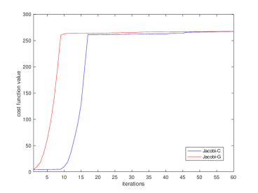
(a) $\boldsymbol{\mathcal{A}}_{1}\in\mathbb{R}^{10\times 10\times 10}$

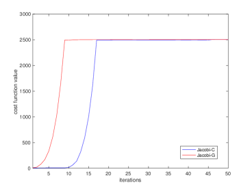
(b) $\boldsymbol{\mathcal{A}}_{2}\in\mathbb{R}^{10\times 10\times 10\times 10}$

​​​

Figure 1: Results of Jacobi-C and Jacobi-G algorithms on $\mathscr{O}_{n}$.

V Conclusion

In this paper, we mainly review our results [10, 21, 16, 22] about the convergence of Jacobi-type algorithms on $\mathscr{O}_{n}$ and $\mathscr{U}_{n}$. For the moment, there are still some open problems:
(i) If $f$ is the cost function in (2) with $d\geq 4$, the global convergence of Algorithm 3 is still unknown.
(ii) The global convergence of Jacobi-C algorithm is still unknown.

References

- [1] P. Comon, “Independent Component Analysis,” in Higher Order Statistics, J.-L. Lacoume, Ed. Amsterdam, London: Elsevier, 1992, pp. 29–38.
- [2] ——, “Independent component analysis, a new concept?” Signal Processing, vol. 36, no. 3, pp. 287–314, 1994.
- [3] L. De Lathauwer, Signal processing based on multilinear algebra. Katholieke Universiteit Leuven Leuven, 1997.
- [4] P. Comon and C. Jutten, Eds., Handbook of Blind Source Separation. Oxford: Academic Press, 2010.
- [5] T. G. Kolda and B. W. Bader, “Tensor decompositions and applications,” SIAM review, vol. 51, no. 3, pp. 455–500, 2009.
- [6] P. Comon, “Tensors: a brief introduction,” IEEE Signal Processing Magazine, vol. 31, no. 3, pp. 44–53, 2014.
- [7] A. Cichocki, D. Mandic, L. D. Lathauwer, G. Zhou, Q. Zhao, C. Caiafa, and H. A. PHAN, “Tensor decompositions for signal processing applications: From two-way to multiway component analysis,” IEEE Signal Processing Magazine, vol. 32, no. 2, pp. 145–163, 2015.
- [8] N. D. Sidiropoulos, L. De Lathauwer, X. Fu, K. Huang, E. E. Papalexakis, and C. Faloutsos, “Tensor decomposition for signal processing and machine learning,” IEEE Transactions on Signal Processing, vol. 65, no. 13, pp. 3551–3582, 2017.
- [9] L. Qi and Z. Luo, Tensor analysis: Spectral theory and special tensors. SIAM, 2017.
- [10] J. Li, K. Usevich, and P. Comon, “Globally convergent Jacobi-type algorithms for simultaneous orthogonal symmetric tensor diagonalization,” SIAM J. Matr. Anal. Appl., vol. 39, no. 1, pp. 1–22, 2018.
- [11] P. Comon, G. Golub, L.-H. Lim, and B. Mourrain, “Symmetric tensors and symmetric tensor rank,” SIAM Journal on Matrix Analysis and Applications, vol. 30, no. 3, pp. 1254–1279, 2008.
- [12] P. Comon, “Tensor Diagonalization, A useful Tool in Signal Processing,” in 10th IFAC Symposium on System Identification (IFAC-SYSID), M. Blanke and T. Soderstrom, Eds., vol. 1. Copenhagen, Denmark: IEEE, Jul. 1994, pp. 77–82.
- [13] L. De Lathauwer, B. De Moor, and J. Vandewalle, “Blind source separation by simultaneous third-order tensor diagonalization,” in 1996 8th European Signal Processing Conference (EUSIPCO 1996), 1996, pp. 1–4.
- [14] ——, “Independent component analysis and (simultaneous) third-order tensor diagonalization,” IEEE Transactions on Signal Processing, vol. 49, no. 10, pp. 2262–2271, 2001.
- [15] J. Cardoso and A. Souloumiac, “Blind beamforming for non-gaussian signals,” IEE Proceedings F (Radar and Signal Processing), vol. 6, no. 140, pp. 362–370, 1993.
- [16] K. Usevich, J. Li, and P. Comon, “Approximate matrix and tensor diagonalization by unitary transformations: convergence of Jacobi-type algorithms,” arXiv:1905.12295v2, 2020.
- [17] B. Jiang, Z. Li, and S. Zhang, “Characterizing real-valued multivariate complex polynomials and their symmetric tensor representations,” SIAM Journal on Matrix Analysis and Applications, vol. 37, no. 1, pp. 381–408, 2016.
- [18] J. Nie and Z. Yang, “Hermitian tensor decompositions,” arXiv preprint arXiv:1912.07175, 2019.
- [19] J.-F. Cardoso and A. Souloumiac, “Jacobi angles for simultaneous diagonalization,” SIAM journal on matrix analysis and applications, vol. 17, no. 1, pp. 161–164, 1996.
- [20] P. Comon, “Contrasts, Independent Component Analysis, and Blind Deconvolution,” International Journal of Adaptive Control and Signal Processing, vol. 18, no. 3, pp. 225–243, 2004.
- [21] J. Li, K. Usevich, and P. Comon, “On approximate diagonalization of third order symmetric tensors by orthogonal transformations,” Linear Algebra and its Applications, vol. 576, pp. 324–351, 2019.
- [22] ——, “Jacobi-type algorithm for low rank orthogonal approximation of symmetric tensors and its convergence analysis,” arXiv:1911.00659, 2019.
- [23] G. Golub and C. Van Loan, Matrix Computations, 3rd ed. Johns Hopkins University Press, 1996.
- [24] S. Łojasiewicz, “Ensembles semi-analytiques,” IHES notes, 1965.
- [25] P. A. Absil, R. Mahony, and B. Andrews, “Convergence of the iterates of descent methods for analytic cost functions,” SIAM Journal on Optimization, vol. 16, no. 2, pp. 531–547, 2005.
- [26] R. Schneider and A. Uschmajew, “Convergence results for projected line-search methods on varieties of low-rank matrices via Lojasiewicz inequality,” SIAM Journal on Optimization, vol. 25, no. 1, pp. 622–646, 2015.
- [27] J. Bolte, S. Sabach, and M. Teboulle, “Proximal alternating linearized minimization for nonconvex and nonsmooth problems,” Mathematical Programming, vol. 146, no. 1-2, pp. 459–494, 2014.
- [28] P.-A. Absil, R. Mahony, and R. Sepulchre, Optimization Algorithms on Matrix Manifolds. Princeton, NJ: Princeton University Press, 2008.
- [29] S. Krantz and H. Parks, A Primer of Real Analytic Functions. Boston: Birkhäuser, 2002.
- [30] M. Ishteva, P.-A. Absil, and P. Van Dooren, “Jacobi algorithm for the best low multilinear rank approximation of symmetric tensors,” SIAM J. Matrix Anal. Appl., vol. 2, no. 34, pp. 651–672, 2013.
- [31] N. Boumal, P.-A. Absil, and C. Cartis, “Global rates of convergence for nonconvex optimization on manifolds,” IMA Journal of Numerical Analysis, vol. 39, no. 1, pp. 1–33, 2019.