BatVision: Learning to See 3D Spatial Layout with Two Ears

Abstract

Many species have evolved advanced non-visual perception while artificial systems fall behind. Radar and ultrasound complement camera-based vision but they are often too costly and complex to set up for very limited information gain. In nature, sound is used effectively by bats, dolphins, whales, and humans for navigation and communication. However, it is unclear how to best harness sound for machine perception.

Inspired by bats’ echolocation mechanism, we design a low-cost BatVision system that is capable of seeing the 3D spatial layout of space ahead by just listening with two ears. Our system emits short chirps from a speaker and records returning echoes through microphones in an artificial human pinnae pair. During training, we additionally use a stereo camera to capture color images for calculating scene depths. We train a model to predict depth maps and even grayscale images from the sound alone. During testing, our trained BatVision provides surprisingly good predictions of 2D visual scenes from two 1D audio signals. Such a sound to vision system would benefit robot navigation and machine vision, especially in low-light or no-light conditions. Our code and data are publicly available.

Figure 1: Our Batvision system learns to generate visual scenes by just listening to echos with two ears. Mounted on a model car, our system has two microphones embedded into artificial human ears, a speaker, and a stereo camera which is only used during training for providing visual image ground-truth. 1) The speaker emits sound chirps in an office space and the microphones receive echos returned from the environment. The camera captures stereo image pairs, based on which depth maps can be calculated. 2) We train a model to turn binaural signals into visual scenes such as depth-maps or grayscale images. Our results show surprisingly accurate reconstruction of the 3D spatial layout of indoor scenes from the input sound alone.

I Introduction

Our task is to train a machine learning system that can turn binaural sound signals to visual scenes. Solving this challenge would benefit robot navigation and machine vision, especially in low-light or no-light conditions.

While many animals sense the spatial layout of the world through vision, some species such as bats, dolphins, and whales rely heavily on acoustic information. For example, bats have advanced ears that give them a form of vision in the dark known as echolocation: They sense the world by continuously emitting ultrasonic pulses and processing echos returned from the environment.

It is indeed possible to locate highly reflecting ultrasonic targets in the 3D space by using an artificial pinnae pair of bats, which acts as complex direction dependent spectral filters and using head related transfer functions  [1, 2].

Likewise, humans who suffer from vision loss have shown to develop capabilities of echolocation using palatal clicks similar to dolphins, learning to sense obstacles in the 3D space by listening to the returning echoes  [3, 4].

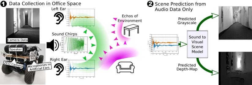
Inspired by bats’ echolocation, we design BatVision that can form a visual image of the 3D world by just listening to the environmental echo sound with two ears (Fig. 1).

Contrary to existing works  [1, 2], our system uses only two simple low-cost consumer-grade microphones to keep it small, mobile, and easily reproducible. Our microphones are embedded into a human pinnae pair to utilize the spectral filters of an emulated human auditory system, which has an additional benefit of easy debugging by human engineers.

Mounted on a model car, our BatVision also has a speaker and a camera which is only used during training for providing visual image ground-truth. Like bats, our speaker emits frequency modulated chirps in the audible spectrum, and our microphones receive echos returned from the environment. Our camera captures stereo image pairs of the scene ahead, from which depth disparity maps can be calculated.

During training, we first collect a dataset of time-synchronized binaural audio signals and stereo image pairs in an indoor office environment, and then train a neural network model to predict images such as depth maps and grayscale images from audio data alone.

During testing, we just need the sound signals to reconstruct depth maps or grayscale images. By just listening with two ears, which receive sound echos at only two points in the 3D space, our BatVision is able to generate a depth map of the 3D space ahead that resolves features such as walls, hallways, door openings, and roughly outlined furniture correctly in azimuth, elevation, and distance, whereas our reconstructed grayscale images show surprisingly plausible floor layouts even though obstacles lack finer details.

For a navigation system, such an intelligent sound system could provide information complementary to vision sensors, independent of light and at very low additional costs. Our approach is conceptually simple, practically easy to implement, and readily deployable on embedded mobile platforms.

To the best of our knowledge, our BatVision is the first work that generates scene depth maps from binaural sound only. Our code, model, and data are available at https://github.com/SaschaHornauer/Batvision.

II Related Works

Biosonar Imaging and Echolocation. Inspired by echolocation in animals, several papers [4, 2, 5, 6, 7] study target echolocation in the 2D or 3D space using ultrasonic frequency modulated (FM) chirps between $20\text{\,}\mathrm{-}$$200\text{\,}\mathrm{kHz}$. Bats emit pulse trains of very short durations (typically $<$5\text{\,}\mathrm{ms}$$) and use received echoes to perceive their surroundings.

In [6, 4], microphones are placed in an artificial bat pinnae to receive the sound signal. The natural form of the bat pinnae acts as a frequency filter, useful for separating spatial information in both azimuth and elevation [8, 2]. These works motivate our use of short FM chirps and artificial human pinnaes with integrated microphones.

In [6], the task is to recognize scenes from echo-cochleogram fingerprints and to create a topological map of the surrounding. In [5], the goal is to autonomously drive a mobile robot while mapping and avoiding obstacles using azimuth and range information from ultrasonic sensors. They classify echo spectrograms into obstacles or not, biological objects or not, along a single scan line and without visual reconstruction of the scene.

In [4], ultrasonic echoes are recorded, dilated, and played back to a human subject in the audible spectrum. After initial training, human subjects were able to pick up echolocation abilities to estimate azimuth, distance, and to some extent, elevation of targets. In [7, 2], 3D targets are localized based on an array of microphones instead of binaural microphones.

Sound Source Localization. In [9, 10, 11, 12, 13], deep neural network models are trained to localize the source of the sound (e.g. a piano) in images or videos. Remarkable results are obtained in a self-supervised learning framework, demonstrating the potential of learning associations between paired audio-visual data.

In [11], sound is localized using an acoustic camera [14], a hybrid audio-visual sensor that provides RGB video overlaid with acoustic sound, aligned in time and space. All the works on sound localization receive sound signals passively.

In [15], sound is localized using emulated binaural hearing, with a model of human ears and head related transfer functions. They test azimuth from $0\text{\,}\mathrm{\SIUnitSymbolDegree}$ to $360\text{\,}\mathrm{\SIUnitSymbolDegree}$ at $5\text{\,}\mathrm{\SIUnitSymbolDegree}$ resolution and test elevation from $-40\text{\,}\mathrm{\SIUnitSymbolDegree}$ to $90\text{\,}\mathrm{\SIUnitSymbolDegree}$ at $10\text{\,}\mathrm{\SIUnitSymbolDegree}$ resolution.

In [16], an audio monologue of a speaker is turned into visual gestures of the speaker’s arms and hands, by translating audio clips into $2D$ trajectories of joint coordinates. Our sound to vision decoder model is inspired by their cross-domain translation success.

Acoustic Imaging. In non-Line-of-Sight imaging [17], a microphone and a speaker array are used to emit and record FM sound waves. The sound waves are chirps in the audible spectrum from $$2\text{\,}\mathrm{Hz}$-$20\text{\,}\mathrm{kHz}$$, emitted to propagate to a wall, a hidden object, and back to the microphone array. They demonstrate successful object reconstruction at a resolution limited by the receiving microphone array. In contrast, we capture the complete scene of the 3D space ahead with a small system mounted on a mobile device.

Figure 2: Data collected at different parts of the building are used for training, validation, and testing. Training and validation data are collected in separate areas of the same floor, whereas the test data come from another floor and have different obstacles and decorations.

III Collection of Our Audio-Visual Dataset

We collect a new dataset of time-synchronized binaural audio, RGB images, and depth maps, which can be used for learning the associations between sound and vision.

III-A Our Data Collection Sites and Splits

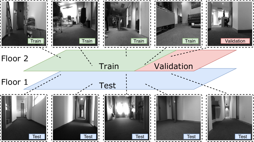
We traverse an office building in the hallways, open areas, conference rooms, and office spaces. We fix our BatVision on a trolley and slowly push it around, so that there is no active motor noise corrupting our sound.

We collect data at various spatial locations to minimize correlation and maximize scene diversity (Fig 2). A total of 39,500 and 7,500 instances at two different parts of the same floor are collected for training and validation respectively, with additional 5,040 instances on a different floor for testing. While hallways appear similar, their spatial layout, furniture, occupancy, and decorations are different.

III-B Our Hardware: Speaker, Ears, and Camera

We use a consumer-grade JBL Flip4 Bluetooth speaker to send out linear FM waveform chirps every half second (Fig. 1). Each chirp sweeps from $$20\text{\,}\mathrm{Hz}$-$20\text{\,}\mathrm{kHz}$$ within a duration of $3\text{\,}\mathrm{ms}$. The waveform characteristics are designed using the freely available software tool Audacity.

We adopt two low-cost consumer-grade omni-directional USB Lavalier MAONO AU-410 microphones, separated at approximately $23.5\text{\,}\mathrm{cm}$ apart. Each microphone is mounted in a Soundlink silicone ear to effectively emulate an artificial human auditory system. We record sound using PyAudio for Python at $44.1\text{\,}\mathrm{kHz}$ and $24\text{\,}$ bits per sample.

We use a ZED camera to capture stereo image pairs and extract depth maps from them. Our camera, speaker, and artificial ears are mounted on a small model car (Fig. 1).

Figure 3: Sample audio waveform and its amplitude spectrogram from a single microphone. The echo appears after the chirp (first peak) at about $3\text{\,}\mathrm{ms}$.

III-C Our Audio clips and Visual Images

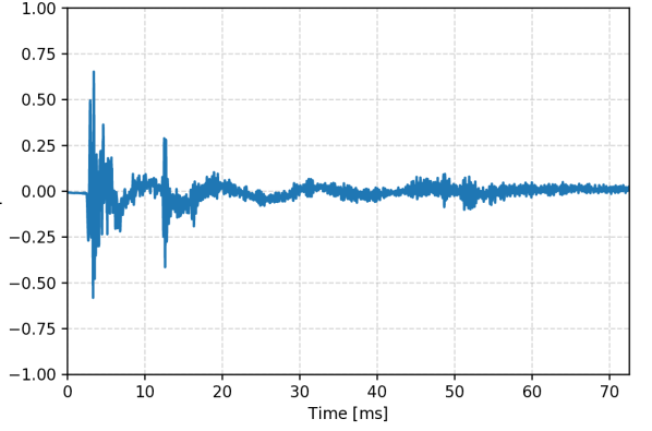
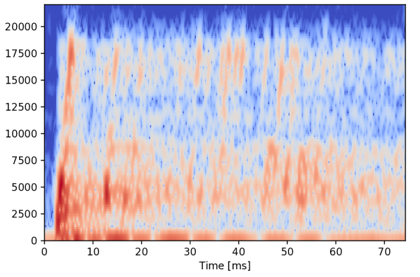
We choose the length of each audio instance to be $72.5\text{\,}\mathrm{ms}$, so that it includes echoes traveling up to $12\text{\,}\mathrm{m}$. This time window selection reflects a trade-off between receiving echos within the distance relevant for navigation and reducing later echos from multiple reflection paths. Each of our audio clips has $3200\text{\,}$ frames, containing one chirp and returned echoes.

We synchronize all the audio instances by the time of the recorded chirp. However, during training, we augment the audio data by jittering the position of the window by 30%.

We consider two audio representations: $1D$ raw waveforms and $2D$ amplitude spectrograms. The LibROSA library for Python is used to compute spectrograms with $512\text{\,}$ points for FFT and Hanning window size $64\text{\,}$. Fig.  3 shows the probing chirp at $3\text{\,}\mathrm{ms}$ and the returned echoes afterwards.

We compute the scene depth using the API of our camera, range clipped within $12\text{\,}\mathrm{m}$. We normalize the depth value to be between 0 and 1. Pixels where the camera is unable to produce a valid measurements are set to 0.

IV Our Sound to Vision Prediction Models

We use an encoder-decoder network architecture to turn the audio clip into the visual image, and further improve the quality of generated images using an adversarial discriminator to contrast them against the ground-truth (Fig. 4).

Figure 4: Our sound to vision network architecture. The temporal convolutional audio encoder $A$ turns the binaural input into a latent audio feature vector, based on which the visual generator $G$ predicts the scene depth map. The discriminator $D$ compares the prediction with the ground-truth and enforces high-frequency structure reconstruction at the patch level.

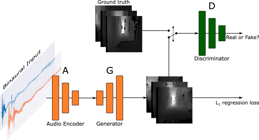
We train our model with two possible audio representations. Our experiments indicate that spectrograms yield slightly better sound-to-vision predictions over raw waveforms. However, as we aim for a real-time BatVision system on embedded platforms, we focus on raw waveforms which are more computationally efficient.

IV-A Our Audio Encoder $A$

Encoder for Waveforms. Following SoundNet [18], we represent the binaural input as two channels of $1D$ signals and transform it into a 1024-dimensional feature vector with 8 temporal convolutions. See Fig. 5 and Table I for details.

Figure 5: Our audio encoder for the raw waveform. We use 8 convolutional layers to turn the two-channel representations of the audio waveform into a 1024-dimensional feature vector.

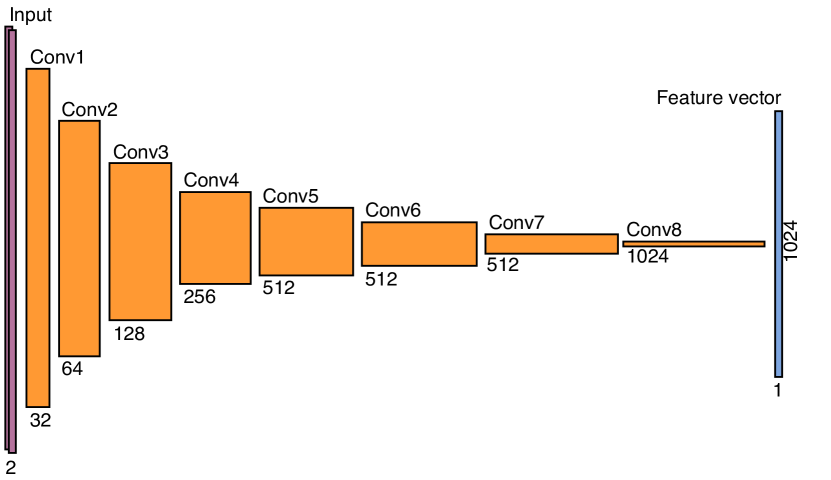
Encoder for Spectrograms. Likewise, with successive temporal convolutions and downsampling, we gradually reduce the time-dimension of the spectrograms down to 1, producing a $1\times f\times 1024$ feature vector, where $f$ is the number of final frequencies. $f$ depends on the downsampling factors along the y-axis of the spectrogram.

TABLE I: Layer configuration of our waveform audio encoder

Layer	# of Filters	Filter size	Stride	Padding
Conv1	32	228	2	114
Conv2	64	128	3	64
Conv3	128	64	3	32
Conv4	256	32	3	16
Conv5	256	16	3	8
Conv6	512	8	3	4
Conv7	512	4	3	2
Conv8	1024	3	3	1

IV-B Our Visual Image Generator $G$

The generator decodes the latent audio feature vector and expands it into visual scene image. For raw waveforms, successive deconvolutions yield the best results, whereas for spectrograms, a UNet-type encoder-decoder network [19] yields best results. We investigate several resolutions for reconstructed images, from $16\times 16$ to $128\times 128$.

Decode by A UNet. To transform the output of our audio encoder to a $2D$ image representation suitable for a UNet, we reshape the 1024-dimensional feature vector into a $32\times 32\times 1$ tensor. For spectrograms, where the audio encoder outputs a $1\times f\times 1024$ vector and $f\neq 1$, we first apply two fully connected linear layers before reshaping it into a $32\times 32\times 1$ tensor. The output of this generator depends on the target resolution, e.g. $128\times 128\times 1$.

The encoder of the UNet downsamples the $32\times 32\times 1$ input through several layers of double convolutions followed by batch normalization and ReLU, whereas the decoder of the UNet upsamples the input through double de-convolutions followed by batch normalization and ReLU. Skip connections are utilized wherever possible.

Decode from Direct Upsampling. Given the $1\times 1\times 1024$ latent audio vector, we apply a series of upsampling layers (as in the UNet decoder) to reach the target resolution. See the layer configuration for the $128\times 128\times 1$ output in Table II.

TABLE II: Layer configuration of the direct upsampling generator for the $128\times 128$ image

Layer	# of Filters	Filter size	Stride	Padding	Res.
Up1	512	4	1	0	4
Up2	512	4	2	1	8
Up3	256	4	2	1	16
Up4	128	4	2	1	32
Up5	128	4	2	1	64
Up6	64	4	2	1	128
Final	1	1	1	0	128

IV-C Our Adversarial Discriminator

We add an adversarial discriminator $D$ for generating more detailed and realistic predictions. We implement the discriminator as a PatchGAN [20] to ensure that the predicted visual image has similar looking patches as the set of ground-truth images; $D$ tries to classify whether each $N\times N$ patch looks real or fake as a ground truth sample, where $N$ is roughly $1/3$ of the image size. $D$ consists of a few convolutional layers with depth, kernel size and stride parameters dependent on the final output image size. See the layer configuration in Table III for size $128\times 128$.

TABLE III: PatchGAN discriminator configuration for $128\times 128$ images.

Layer	# of Filters	Filter size	Stride	Padding
Conv1	64	4	2	1
Conv2	128	4	2	1
Conv3	256	4	2	1
Conv4	1	4	2	1

Figure 6: Sample sound-to-vision predictions by Generator $G$ only without the adversarial discriminator $D$. Columns 1-2 show the grayscale scene image and the ground-truth depth map. The rest columns show predictions from waveforms and spectrograms at size $16\times 16$, $32\times 32$, $64\times 64$, and $128\times 128$.

V Experimental Results

V-A Generator Only Without Discriminator

In a preliminary study that compares input modes and fusion design choices, we predict small images at size $16\times 16$. We have the following observations.

• For raw waveforms, early fusion (left-right-channel concatenation of the input audio) outperforms late fusion (concatenation at Conv8, see Fig. 5).

• Spectrograms yield slightly better results than raw waveforms.

However, as we aim for real-time performance on embedded platforms, we focus on the least computationally expensive method using waveforms.

We compute the prediction error via an $L_{1}$ regression loss:

$$\mathcal{L}_{L_{1}}(G)=\mathbb{E}_{x,y}\left[||y-G(A(x))||_{1}\right]$$ (1)

where $x$ is the audio waveforms or spectrograms, $y$ is the ground truth visual image (depth map or grayscale scene image), $A$ is the audio encoder, and $G$ is the generator.

We use leaky ReLU with slope $0.2$, batch size $16$, and Adam solver [21] with an initial learning rate of $1\times 10^{-4}$ with parameters $\beta_{1}$ and $\beta_{2}$ set to $0.9$ and $0.999$ respectively.

Table IV compares various model choices along with two trivial reconstruction baselines which do not learn any sound and vision associations at all:

1. The mean depth map of the training set.

2. Random uniform noise in the $\left[0,1\right)$ range.

For raw waveforms, direct upsampling and early fusion perform the best. For spectrograms, early fusion, downsampling to $1\times 10\times 1024$ and the UNet generator perform best. These two best configurations are retrained for output dimensions of $32\times 32$, $64\times 64$ and $128\times 128$, and the loss is higher for a larger depth map (Table V).

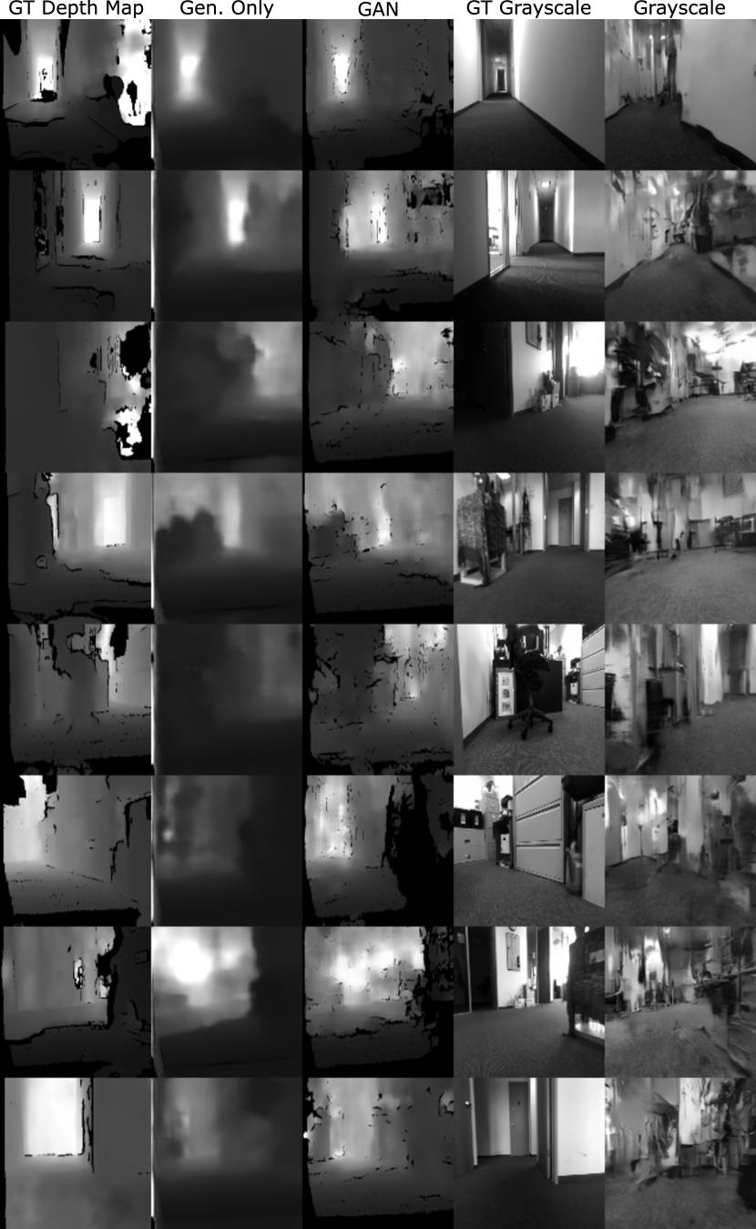
Fig. 6 compares reconstructions at different resolutions. Fig. 7 shows more samples of diverse scenes at reconstruction size $128\times 128$. The sound-to-vision predictions provide a rough outline of the spatial layout of the 3D scene.

TABLE IV: “Generator Only” results for $16\times 16$ imgs. on the test set.

Audio Encoder	Fusion	Shape	Generator	Loss
Waveform	Early	1024	UNet	0.0883
			Direct	0.0838
	Late	1024	UNet	0.0894
			Direct	0.0845
Spectrogram	Early	1024	UNet	0.0834
			Direct	0.0790
		$1\times 10\times 1024$	UNet	0.0773
			Direct	0.0778
Mean Depth				0.1058
Random Noise				0.3654

V-B Generator with Adversarial Discriminator

We use an Generative Adversarial network (GAN) model at the patch level to improve the visual reconstruction quality. We use the following least-squares loss instead of a sigmoid cross-entropy loss in order to avoid vanishing gradients [22]:

$$\mathcal{L}_{GAN}(D)\!=\!\mathbb{E}_{y}\left[\|1-D(y)\|^{2}_{2}\right]\!+\!\mathbb{E}_{x}\left[\|D(G(A(x)))\|^{2}_{2}\right]$$ (2)

$$\mathcal{L}_{GAN}(G)\!=\!\mathbb{E}_{x}\left[\|1-D(G(A(x)))\|^{2}_{2}\right]$$ (3)

Our full objective is thus:

$$\min_{G}\max_{D}\quad\frac{1}{2}\mathcal{L}_{GAN}(D)+\mathcal{L}_{GAN}(G)+\lambda\mathcal{L}_{L_{1}}(G)$$ (4)

where $\lambda$ is a weight factor. We use leaky ReLU with slope 0.2, $\lambda=100$, batch size $16$, and Adam solver with learning rate set to $2\times 10^{-4}$ with parameters $\beta_{1}$ and $\beta_{2}$ set to $0.5$ and $0.999$ respectively.

Figure 7: Good test sample reconstructions at the $128\times 128$ output resolution. Columns 1 and 4 show the ground truth depth map and grayscale scene image. The remaining columns show predictions from raw waveforms. Overall, our generated depth maps show correct mapping of close and distant areas even for row 3, where errors are present in the ground-truth itself.

Figure 8: Poor test sample reconstructions. Same conventions as Fig. 7. Up-close and complex objects are not well represented.

TABLE V: $L_{1}$ test loss for waveforms and spectrograms at resolution $32\times 32$, $64\times 64$, and $128\times 128$

Model	Waveform (D. Upsampling)			Spectrogram (UNet Style)
	32	64	128	32	64	128
Gen. Only
Depth map	0.0852	0.0862	0.0880	0.0722	0.0726	0.0742
GAN
Depth map	0.0867	0.0955	0.0930	0.0799	0.0808	0.0878
Grayscale	0.2238	0.1967	0.2018	0.1721	0.1845	0.1841

Table V compares the test set loss over a few design choices. As in the ”Generator Only” case, the loss is moderately higher for a larger depth map. However, Fig. 7 shows our sample reconstructions by GAN have much finer details and clearer borders, and our grayscale reconstructions in the rightmost column have well placed floors even though objects are roughly outlined and abstracted.

V-C Limitations of Our Approach

How sound resonates, propagates and reflects in a room has a huge impact on sound-to-vision predictions.

• Some materials have dampening properties, leading to faint or absorbed echos.

• Facing corners, where hallways fork in different directions, poses a big challenge, because sound waves scatter off in different directions.

• At short ranges (e.g. <$1\text{\,}\mathrm{m}$), multi-path echoes could be received at the same time with similar amplitudes, creating a superposition that is difficult to resolve.

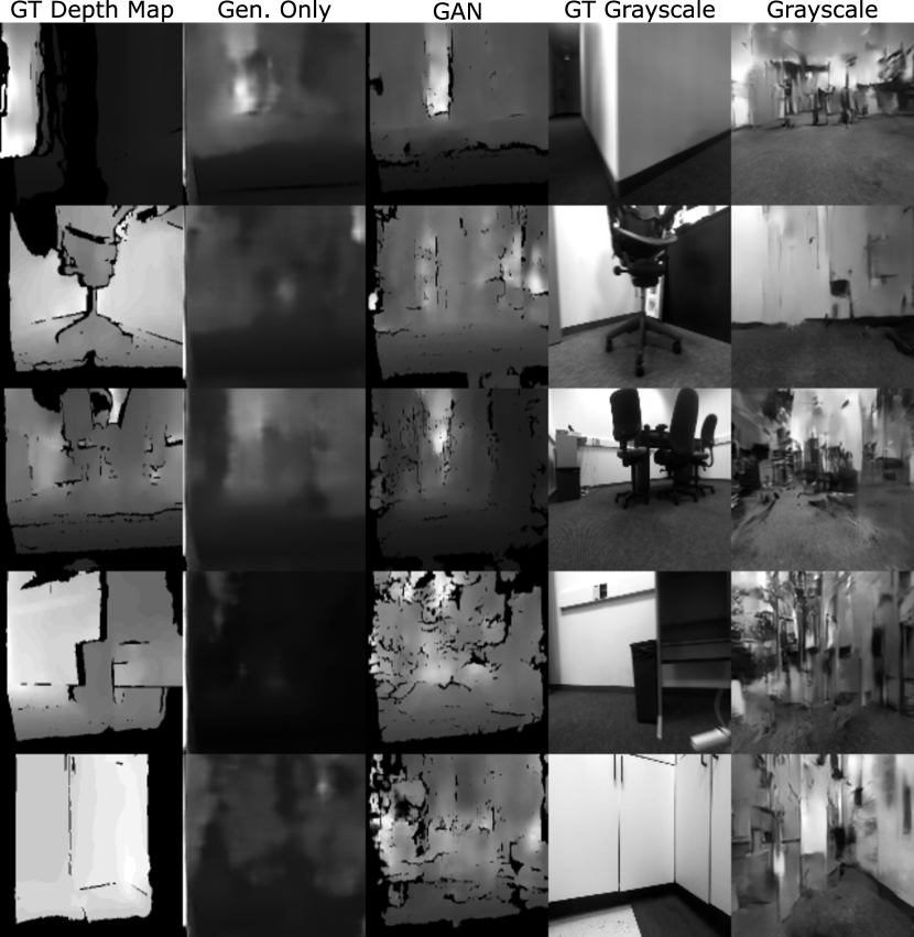
• In areas with dense obstacles such as conference rooms with many office chairs, our sound-to-vision model often fails to predict any meaningful content (Fig. 8).

VI Conclusions

Our BatVision system with a trained sound-to-vision model can reconstruct depth maps from binaural sound recorded by only two microphones to a remarkable accuracy. It can predict detailed indoor scene depth and obstacles such as walls and furniture. Sometimes, it even outperforms our ground-truth depth map obtained from a stereo vision algorithm which struggles to estimate disparity reliably.

Generating the grayscale scene image is more difficult; the amount of detail and information required is not expected to be present in sound echos. However, our trained model is able to generate plausible wall placements and free floor areas. When objects are not recognizable from the sound, the network fills in with an approximation of obstacles.

Such seemingly incredible sound-to-vision results reflect natural statistical correlations between the sound and the image of indoor scenes, captured by our model trained on diverse scenes and likely utilized in a similar fashion by humans and animals.

References

- [1] F. Schillebeeckx, F. De Mey, D. Vanderelst, and H. Peremans, “Biomimetic sonar: Binaural 3d localization using artificial bat pinnae,” I. J. Robotic Res., vol. 30, pp. 975–987, 07 2011.
- [2] I. Matsuo, J. Tani, and M. Yano, “A model of echolocation of multiple targets in 3d space from a single emission,” The Journal of the Acoustical Society of America, vol. 110, no. 1, pp. 607–624, 2001. [Online]. Available: https://doi.org/10.1121/1.1377294
- [3] R. Kuc and V. Kuc, “Modeling human echolocation of near-range targets with an audible sonar,” The Journal of the Acoustical Society of America, vol. 139, pp. 581–587, 02 2016.
- [4] J. Sohl-Dickstein, S. Teng, B. Gaub, C. C. Rodgers, C. Li, M. R. DeWeese, and N. S. Harper, “A device for human ultrasonic echolocation,” IEEE transactions on bio-medical engineering, vol. 62, 01 2015.
- [5] I. Eliakim, Z. Cohen, G. Kósa, and Y. Yovel, “A fully autonomous terrestrial bat-like acoustic robot,” PLOS Computational Biology, vol. 14, p. e1006406, 09 2018.
- [6] J. Steckel and H. Peremans, “Batslam: Simultaneous localization and mapping using biomimetic sonar,” PloS one, vol. 8, p. e54076, 01 2013.
- [7] B. Fontaine, H. Peremans, and J. Steckel, “3d sparse imaging in biosonar scene analysis,” 04 2009.
- [8] J. M. Wotton and J. A. Simmons, “Spectral cues and perception of the vertical position of targets by the big brown bat, eptesicus fuscus,” The Journal of the Acoustical Society of America, vol. 107, no. 2, pp. 1034–1041, 2000. [Online]. Available: https://doi.org/10.1121/1.428283
- [9] Y. Tian, J. Shi, B. Li, Z. Duan, and C. Xu, “Audio-visual event localization in the wild,” Proc. CVPR Workshop: Sight and Sound, 06 2019.
- [10] A. Senocak, T. Oh, J. Kim, M. Yang, and I. S. Kweon, “Learning to localize sound source in visual scenes,” CoRR, vol. abs/1803.03849, 2018. [Online]. Available: http://arxiv.org/abs/1803.03849
- [11] A. F. Pérez, V. Sanguineti, P. Morerio, and V. Murino, “Audio-visual model distillation using acoustic images,” 04 2019.
- [12] A. Ephrat, I. Mosseri, O. Lang, T. Dekel, K. Wilson, A. Hassidim, W. T. Freeman, and M. Rubinstein, “Looking to listen at the cocktail party: A speaker-independent audio-visual model for speech separation,” ACM Trans. Graph., vol. 37, no. 4, pp. 112:1–112:11, July 2018. [Online]. Available: http://doi.acm.org/10.1145/3197517.3201357
- [13] A. Owens and A. A. Efros, “Audio-visual scene analysis with self-supervised multisensory features,” arXiv preprint arXiv:1804.03641, 2018.
- [14] A. Zunino, M. Crocco, S. Martelli, A. Trucco, A. Del Bue, and V. Murino, “Seeing the sound: A new multimodal imaging device for computer vision,” 2015 IEEE International Conference on Computer Vision Workshop (ICCVW), 12 2015.
- [15] F. Keyrouz and K. Diepold, “An enhanced binaural 3d sound localization algorithm,” in 2006 IEEE International Symposium on Signal Processing and Information Technology, Aug 2006, pp. 662–665.
- [16] S. Ginosar, A. Bar, G. Kohavi, C. Chan, A. Owens, and J. Malik, “Learning individual styles of conversational gesture,” in Computer Vision and Pattern Recognition (CVPR). IEEE, June 2019.
- [17] D. B. Lindell, G. Wetzstein, and V. Koltun, “Acoustic non-line-of-sight imaging,” Proc. CVPR, 2019.
- [18] Y. Aytar, C. Vondrick, and A. Torralba, “Soundnet: Learning sound representations from unlabeled video,” in Advances in Neural Information Processing Systems 29, D. D. Lee, M. Sugiyama, U. V. Luxburg, I. Guyon, and R. Garnett, Eds. Curran Associates, Inc., 2016, pp. 892–900. [Online]. Available: http://papers.nips.cc/paper/6146-soundnet-learning-sound-representations-from-unlabeled-video.pdf
- [19] O. Ronneberger, P. Fischer, and T. Brox, “U-net: Convolutional networks for biomedical image segmentation,” in Medical Image Computing and Computer-Assisted Intervention – MICCAI 2015, N. Navab, J. Hornegger, W. M. Wells, and A. F. Frangi, Eds. Cham: Springer International Publishing, 2015, pp. 234–241.
- [20] P. Isola, J.-Y. Zhu, T. Zhou, and A. Efros, “Image-to-image translation with conditional adversarial networks,” 07 2017, pp. 5967–5976.
- [21] D. Kingma and J. Ba, “Adam: A method for stochastic optimization,” International Conference on Learning Representations, 12 2014.
- [22] X. Mao, Q. Li, H. Xie, R. Y. K. Lau, Z. Wang, and S. P. Smolley, “Least squares generative adversarial networks,” in 2017 IEEE International Conference on Computer Vision (ICCV), Oct 2017, pp. 2813–2821.