Efficient quantum algorithm for solving structured problems via multi-step quantum computation

Abstract

In classical computation, a problem can be solved in multiple steps where calculated results of each step can be copied and used repeatedly. While in quantum computation, it is difficult to realize a similar multi-step computation process because the no-cloning theorem forbids making copies of an unknown quantum state perfectly. We find a method based on quantum resonant transition to protect and reuse an unknown quantum state that encodes calculated results of an intermediate step without making copies of the state, and present a quantum algorithm that solves a problem via a multi-step quantum computation process. This algorithm can achieve an exponential speedup over classical algorithms in solving a type of structured search problems.

I Introduction

Solving a problem on a quantum computer can be transformed to finding the ground state of a problem Hamiltonian that encodes the solution to the problem. The phase estimation algorithm (PEA) kitaev ; abrams projects an initial state onto the ground state of the problem Hamiltonian with probability proportional to the square of the overlap between them. However, it is difficult to find a good initial state for a complicated system. By using amplitude amplification, quantum algorithms can achieve quadratic speed-up over classical algorithms in preparing the ground state of a quantum many-body system poulin1 . In adiabatic quantum computing (AQC) farhi1 , the system is evolved adiabatically from the ground state of an initial Hamiltonian to that of the problem Hamiltonian. The efficiency of AQC depends on the minimum energy gap between the ground and the first excited states of the adiabatic Hamiltonian, which is difficult to estimate in most cases. Quantum Zeno effect childs ; poulin can be used to keep a quantum computer near ground state of a smoothly varying Hamiltonian by performing frequent measurements, and has the same efficiency as AQC.

The structure of a problem is the key for whether it can be solved efficiently or not on a quantum computer. In Refs. struct ; structAQC , a nested search algorithm was proposed for problems that can be divided into two (or more) levels described by a set of primary and secondary variables, respectively. It works by nesting one quantum search within another, and performing quantum search at a selected level among partial solutions to narrow subsequent search over their descendants. The complete solution is constructed through a tree of partial solutions at different levels. This algorithm achieves quadratic speedup over the corresponding classical nesting algorithms, and can be faster than the usual Grover bound for unstructured search. In general, the constraints of a problem contain variables that are coupled to each other, the variables may be divided into only a few sets, thus the search space is still exponentially large.

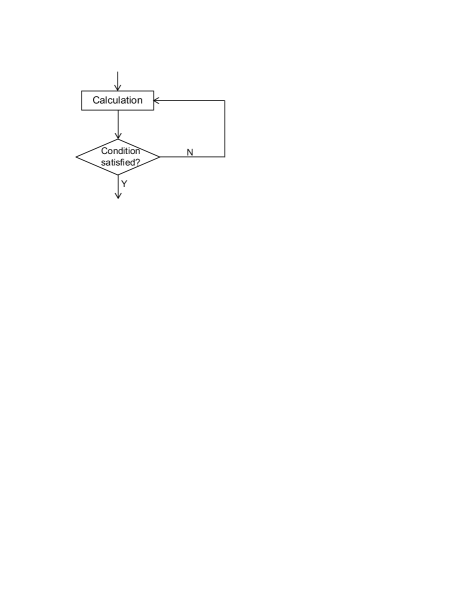
Figure 1: Flowchart for one step in a multi-step computation process.

In the circuit model, a quantum computation is performed by first preparing qubits in an initial state, then applying a series of unitary operations, finally measuring the qubits to obtain calculation results. While in classical computation, a problem can be solved in multiple steps, where each step contains a computation procedure as shown in Fig. $1$: with calculated results of the previous step as input, one performs a calculation, then checks if the results satisfy certain conditions; if the conditions are satisfied, then continue calculation of the next step, otherwise, repeat the procedure iteratively until the desired results are obtained. This process is easy to implement in classical computation since calculated results of each step can be copied and used repeatedly, the runtime is proportional to the number of computation steps. In quantum computation, however, it is difficult to realize a similar multi-step quantum computation process due to the restriction of the no-cloning theorem noclone1 ; noclone2 , which forbids making copies of an unknown quantum state perfectly. Calculated results encoded in an unknown quantum state cannot be used by making copies as in classical computation. Therefore in multi-step quantum computation, if one fails to obtain desired results of a step, one has to run the algorithm from beginning again. This leads to the result that the runtime scales exponentially with the number of steps of the algorithm.

We find a method to protect and reuse an unknown quantum state that encodes calculated results of an intermediate step without copying it. Using this method, we present a quantum algorithm for finding the ground state of a problem Hamiltonian via multi-step quantum computation. And apply it for efficiently solving a type of structured search problems that can be decomposed in a more general way than that of in Refs. struct ; structAQC , in which the search space of the problems is reduced in polynomial rate to the target state, while it is difficult to solve them through the usual quantum computation process.

The idea of the algorithm is as follows: we construct an evolution path from an initial Hamiltonian $H_{0}$ to a problem Hamiltonian $H_{P}$ by inserting between them a sequence of intermediate Hamiltonians {$H_{l},$ $l\!=\!1,\cdots,m\!-\!1$}, through which $H_{0}$ reaches $H_{P}$ as $H_{0}\rightarrow H_{1}\rightarrow\cdots\rightarrow H_{m-1}\rightarrow H_{P}\!=\!H_{m}$. We start from the ground state $|\varphi_{0}^{(0)}\rangle$ of $H_{0}$, and evolve it through ground states of the intermediate Hamiltonians sequentially to reach the ground state $|\varphi_{0}^{(m)}\rangle$ of $H_{P}$ in $m$ steps. In each step, ground state of an intermediate Hamiltonian is obtained deterministically via quantum resonant transitions (QRT) whf0 ; whf2 . For Hamiltonians that can be simulated efficiently on a quantum computer, the algorithm can be run efficiently if: $i$) overlaps between ground states of any two adjacent Hamiltonians and, $ii$) energy gap between the ground and the first excited states of each Hamiltonian, are not exponentially small. The conditions can be reduced to simpler form for problems with special structures.

Compared with the algorithm in Ref. childs , our algorithm is flexible in designing evolution paths. As we demonstrate later, our algorithm can solve a type of structured search problems efficiently through a path even when the usual AQC algorithm, which has the same efficiency as the algorithm in childs , fails following the same path.

II The algorithm

We describe the algorithm by using one of its steps as example. By optimizing the algorithm in whf0 ; whf2 , one qubit is saved in this algorithm. It requires $\left(n+1\right)$ qubits with one probe qubit and an $n$-qubit register $R$ representing a problem of dimension $N=2^{n}$. In the $l$-th step, given the Hamiltonians $H_{l}$, $H_{l-1}$ and its ground state $|\varphi_{0}^{\left(l-1\right)}\rangle$ prepared on register $R$ and the corresponding eigenvalue $E_{0}^{\left(l-1\right)}$ obtained from previous step, we aim to prepare the ground state $|\varphi_{0}^{\left(l\right)}\rangle$ and obtain the corresponding eigenvalue $E_{0}^{\left(l\right)}$ of $H_{l}$. The algorithm Hamiltonian of the $l$-th step is

$$H^{\left(l\right)}=-\frac{1}{2}\omega\sigma_{z}\otimes I_{N}+H_{R}^{\left(l\right)}+c\sigma_{x}\otimes I_{N},$$ (1)

where

$$H_{R}^{\left(l\right)}=\alpha_{l}|1\rangle\langle 1|\otimes H_{l-1}+|0\rangle\langle 0|\otimes H_{l}\mathbf{,}\text{\ }l=1,2,\cdots,m,$$ (2)

$I_{N}$ is the $N$-dimensional identity operator, and $\sigma_{x,\text{ }z}$ are the Pauli matrices. The first term in Eq. ($1$) is the Hamiltonian of the probe qubit, the second term contains the Hamiltonian of the register $R$ and describes the interaction between the probe qubit and $R$, and the third term is a perturbation. The parameter $\alpha_{l}$ is used to rescale energy levels of $H_{l-1}$, and the ground state energy of $\alpha_{l}H_{l-1}$ is used as a reference point to the ground state eigenvalue of $H_{l}$, and $c\ll 1$. We estimate the range of the ground state eigenvalue $E_{0}^{\left(l\right)}$ of $H_{l}$ and obtain the estimated transition frequency range $\left[\omega_{\min}\text{, }\omega_{\max}\right]$ between states $|\varphi_{0}^{\left(l-1\right)}\rangle$ and $|\varphi_{0}^{\left(l\right)}\rangle$. Then discretize the frequency range into a number of grids and use them as detection frequency of the probe qubit. Procedures of the $l$-th step of the algorithm are as follows:

$i$) Set the probe qubit in a frequency from the frequency set, and initialize it in its excited state $|1\rangle$ and the register $R$ in state $|\varphi_{0}^{\left(l-1\right)}\rangle$.

$ii$) Implement the time evolution operator $U(t)=\exp\left(-iH^{\left(l\right)}t\right)$.

$iii$) Read out the state of the probe qubit.

We repeat procedures $ii$)-$iii$) a number of times. If the measurement on the probe qubit results in state $|1\rangle$, it indicates that register $R$ remains in state $|\varphi_{0}^{\left(l-1\right)}\rangle$, then we run procedures $ii$)-$iii$) by setting the probe qubit in another frequency. Otherwise if the probe qubit decays to state $|0\rangle$, it indicates a resonant transition from state $|1\rangle|\varphi_{0}^{\left(l-1\right)}\rangle$ to $|0\rangle|\varphi_{0}^{\left(l\right)}\rangle$. The eigenvalue $E_{0}^{\left(l\right)}$ of $H_{l}$ can be obtained by locating resonant transition frequency of the probe qubit that satisfies $E_{0}^{\left(l\right)}-\alpha_{l}E_{0}^{\left(l-1\right)}=\omega$. The corresponding eigenvector $|\varphi_{0}^{\left(l\right)}\rangle$ can be prepared by running the above procedure at the resonant transition frequency whf0 ; whf2 . With $H_{l}$, $|\varphi_{0}^{\left(l\right)}\rangle$ and $E_{0}^{\left(l\right)}$, we run the algorithm for next step. Proceeding step by step, finally we obtain the ground state of the problem Hamiltonian. For some problems, the ground state eigenvalues of the intermediate Hamiltonians can be calculated analytically, implementation of the algorithm becomes easier.

As resonant transition occurs, the system is approximately in state $\sqrt{1-p_{0}^{\left(l\right)}}|1\rangle|\varphi_{0}^{\left(l-1\right)}\rangle+\sqrt{p_{0}^{\left(l\right)}}|0\rangle|\varphi_{0}^{\left(l\right)}\rangle$, where $p_{0}^{\left(l\right)}=\sin^{2}\left(ctd_{0}^{(l)}\right)$ is the decay probability of the probe qubit of $l$-th step, and $d_{0}^{(l)}=\langle\varphi_{0}^{(l-1)}|\varphi_{0}^{(l)}\rangle$. The state $|\varphi_{0}^{\left(l-1\right)}\rangle$ is protected in this entangled state. If measurement performed on the probe results in state $|0\rangle$, it indicates the state $|\varphi_{0}^{\left(l\right)}\rangle$ is obtained on register $R$, then we run ($l+1$)-th step of the algorithm. Otherwise if the probe is in state $|1\rangle$, it means $R$ remains in state $|\varphi_{0}^{\left(l-1\right)}\rangle$, we repeat procedures $ii$)-$iii$) by setting the probe in the resonant transition frequency until it decays to state $|0\rangle$. By protecting calculated results of an intermediate step in this entangled state, we do not need to run the algorithm from beginning once it fails to obtain the desired state in a step of the algorithm. We just repeat procedures of the step until the desired state is obtained. With this property, desired state of each step is obtained deterministically in polynomial time if the conditions of the algorithm are satisfied. Here “deterministically” means that by running the procedures of a step repeatedly, we know exactly when the desired state of the step is obtained from the outcome of measurement on the probe qubit. The number of times the procedures have to be repeated is proportional to $1/p_{0}^{\left(l\right)}$. Therefore, runtime of the algorithm is proportional to $\sum_{l=1}^{m}1/p_{0}^{\left(l\right)}$, which scales linearly with the number of steps of the algorithm, provided $p_{0}^{\left(l\right)}$ are not exponentially small.

There are various ways to construct evolution paths that satisfy conditions of the algorithm. Here we present two methods: $i$) for a system Hamiltonian $H_{0}+V$, by writing $H=H_{0}+gV$ ($g\in\left[0,1\right]$) and discretizing the parameter $g$, intermediate Hamiltonians $H_{l}=H_{0}+g_{l}V$ ($0=g_{0}<g_{1}<\cdots<g_{m}=1$) can be constructed poulin . The parameters $g_{l}$ can be adjusted to make $d_{0}^{(l)}$ finite; $ii$) the system Hamiltonian can be a Hamiltonian matrix, intermediate Hamiltonian matrices can be constructed by spanning the system Hamiltonian in a sequence of basis sets with increasing dimension, such that the matrix $H_{l-1}$ is contained in a subspace of the following matrix $H_{l}$. The dimension of the basis sets can be adjusted to make $d_{0}^{(l)}$ to be finite. The path can also be constructed considering the structure of the problem as below.

In $l$-th step, the probability of the initial state being evolved to the state $|0\rangle|\varphi_{0}^{\left(l\right)}\rangle$ reaches maximum at $t=\pi/(2cd_{0}^{(l)})$. Errors are introduced as the initial state leaks to the excited states $|0\rangle|\varphi_{j}^{(l)}\rangle$ ($j=1,\ldots,N-1$) with probability $p_{j}$. By assuming $E_{1}^{(l)}-E_{0}^{(l)}\gg cd_{0}^{(l)}$ and $\alpha_{l}(E_{1}^{(l-1)}-E_{0}^{(l-1)})\gg cd_{0}^{(l)}$, and set the optimal runtime $t=\pi/(2cd_{0}^{(l)})$ for convenience, we have

$$\sum_{j}p_{j}\leq a_{l}^{2}c^{2},$$ (3)

where

$$a_{l}^{2}=\frac{4\left[1-\left(d_{0}^{(l)}\right)^{2}\right]}{\left[E_{1}^{(l)}-\!E_{0}^{(l)}\right]^{2}}.$$

(see Appendix A for details). If the energy gap $E_{1}^{\left(l\right)}-E_{0}^{\left(l\right)}$ are not exponentially small, i.e., bounded by a polynomial function of the problem size, then $a_{l}$ is finite and the error in the $l$-th step is bounded by $a_{l}^{2}c^{2}$. Considering errors accumulated in all steps, the success probability of the algorithm satisfies

$$P_{\text{succ}}\geqslant\prod_{l=1}^{m}\left[1-a_{l}^{2}c^{2}\right]\geqslant\left[1-\left(a_{\max}c\right)^{2}\right]^{m},$$

where $a_{\max}$ is the maximum value of $a_{l}$. The coefficient $c$ can be set such that $a_{\max}c<1/\sqrt{m}$, then $P_{\text{succ}}>1/e$ in the asymptotic limit of $m$. The runtime of each step is proportional to $\pi/(2cd_{0}^{(l)})$, therefore the runtime of the algorithm scales as $O\left(\sum_{l=1}^{m}\frac{\pi}{2(E_{1}^{(l)}-E_{0}^{(l)})d_{0}^{(l)}}\right)$.

We need to find the accurate ground state eigenvalues of the intermediate Hamiltonians, and do not need to know the accurate overlap $d_{0}^{(l)}$ between the ground states of two adjacent Hamiltonians, the algorithm can be performed by using an estimated instead of the optimal runtime. These will cause extra cost, but the scaling is the same, which is proportional to the number of steps of the algorithm (see Appendix A).

The time evolution operators $U(t)=\exp\left(-iH^{\left(l\right)}t\right)$ can be implemented efficiently using Hamiltonian simulation algorithms QSP ; qubitization for simulatable Hamiltonians. Our algorithm requires performing a single-qubit measurement and resetting the probe qubit to its excited state, such techniques have been realized in ion-trap experiment qubit . We now apply the algorithm for solving a type of structured search problems.

III Search problem with a special structure

The unstructured search problem is to find a marked item in an unsorted database of $N$ items using an oracle that recognizes the marked item. The oracle is defined in terms of a problem Hamiltonian $H_{P}=-|q\rangle\langle q|$, where $|q\rangle$ is the marked state associated with the marked item. The initial Hamiltonian is defined as $H_{0}=-|\psi_{0}\rangle\langle\psi_{0}|$, where $|\psi_{0}\rangle=\frac{1}{\sqrt{N}}\sum_{j=0}^{N-1}|j\rangle$. We consider a structured search problem that can be decomposed by using $m$ (in order of $O\left(\log N\right)$) oracles to construct a sequence of intermediate Hamiltonians

$$H_{i}=\frac{N_{i}}{N}H_{0}+\left(1-\frac{N_{i}}{N}\right)H_{P_{i}},\text{ \ \ }i=1,2,\cdots,m-1,$$ (4)

where

$$H_{P_{i}}=-\sum_{q_{i}\in\Pi_{i}}|q_{i}\rangle\langle q_{i}|,$$ (5)

and $H_{m}=H_{P}$ and $\Pi_{m}$ only contains the target state $|q\rangle$, and $\Pi_{1}\supset\cdots\supset\Pi_{m-1}\supset\Pi_{m}$ with sizes $N_{1}$, $\cdots$, $N_{m-1}$, $N_{m}=1$, respectively. If $N_{i}/N_{i-1}$ ($i=1,2,\cdots,m$) are not exponentially small, the problem can be solved efficiently in $m$ steps by using our algorithm.

Define $|q_{i}^{\bot}\rangle=\frac{1}{\sqrt{N-N_{i}}}\sum_{j\notin\Pi_{i}}|j\rangle$. In basis $\left(\left\{|q_{i}\rangle\right\}_{q_{i}\in\Pi_{i}}\text{, }|q_{i}^{\bot}\rangle\right)$, the Hamiltonian $H_{i}$ in Eq. ($4$) can be written as

$$H\!_{i}\!\!=\!\!\left(\!\!\begin{array}[]{cccc}\frac{\xi-1}{N}&\cdots&\frac{\xi-1}{N}&\frac{\left(\xi\!-\!1\right)\!\sqrt{\!N\!-\!N_{i}}}{N}\\ \vdots&\ddots&\vdots&\vdots\\ \frac{\xi-1}{N}&\cdots&\frac{\xi-1}{N}&\frac{\left(\xi-1\right)\!\sqrt{N\!-\!N_{i}}}{N}\\ \frac{\left(\!\xi\!-\!1\!\right)\!\sqrt{\!N\!-\!N_{i}}}{N}&\cdots&\frac{\left(\!\xi\!-\!1\!\right)\!\sqrt{\!N\!-\!N_{i}}}{N}&\xi^{2}\end{array}\!\!\right)\!-\!\xi I_{N_{i}+1},$$ (6)

where $\xi=1-\frac{N_{i}}{N}$ and $I_{N_{i}+1}$ is the identity matrix of dimension $N_{i}+1$. The eigenvalues of the ground and the first excited states of $H_{i}$ are $E_{\pm}^{\left(i\right)}=\frac{-1\pm\Delta E_{i}}{2}$, respectively, where $\Delta E_{i}\!=\!\sqrt{\!\left(\!1\!-\!\frac{2N_{i}}{N}\!\right)^{2}\!+\!4\frac{N_{i}^{2}}{N^{2}}\left(\!1\!-\!\frac{N_{i}}{N}\!\right)}$ is the energy gap between them and reaches minimum $\sqrt{11}/3\sqrt{3}\approx 0.638$ at $N_{i}/N=1/3$. Let $\mathbf{e}=\left(1,\cdots,1\right)^{\text{T}}$ and $\mathbf{0}=\left(0,\cdots,0\right)^{\text{T}}$ be $N_{i}\times 1$ vectors, respectively, there are $N_{i}-1$ degenerate eigenstates $|e_{i}^{\prime}\rangle=\left(|e_{i}^{\perp}\rangle,0\right)^{\text{T}}$ of $H_{i}$ with eigenvalue $-\xi$, where $|e_{i}^{\perp}\rangle$ is orthogonal to $\mathbf{e}$. These eigenstates are uncoupled from the ground and the first excited states of $H_{i}$ cerf . The condition for resonant transition between states $|1\rangle|V_{-}^{\left(i-1\right)}\rangle$ and $|0\rangle|V_{-}^{\left(i\right)}\rangle$ is satisfied by setting $\omega=1$ and $\alpha_{i}=\left(E_{-}^{\left(i\right)}-1\right)/E_{-}^{\left(i-1\right)}$. The ground state of $H_{i}$ is $|V_{-}^{\left(i\right)}\rangle=x_{1}^{\left(i\right)}\left(\mathbf{e},0\right)^{\text{T}}+x_{2}^{\left(i\right)}\left(\mathbf{0},1\right)^{\text{T}}$. After normalization, the overlap between the ground states of two adjacent intermediate Hamiltonians is

$$d_{0}^{(i)}\! = \!\langle V_{-}^{\left(i\!-\!1\right)}|V_{-}^{\left(i\right)}\rangle\!=\!\sqrt{\frac{N_{i}}{N_{i-1}}}x_{1}^{\left(i\!-\!1\right)\ast}x_{1}^{\left(i\right)}\!+$$ (7)

$$\!\frac{N_{i\!-\!1}\!-\!N_{i}}{\sqrt{\!N_{i\!-\!1}(N\!\!-\!\!N_{i})}}x_{1}^{\left(i\!-\!1\right)\ast}x_{2}^{(i)}\!\!+\!\!\sqrt{\!\!\frac{N\!\!-\!\!N_{i\!-\!1}}{N\!\!-\!\!N_{i}}}\!x_{2}^{\left(i\!-\!1\!\right)\ast}\!x_{2}^{\left(i\right)}.$$

The components $x_{1}^{\left(i\right)}$ and $x_{2}^{\left(i\right)}$ are functions of $N_{i}/N$, and $x_{1}^{\left(i\right)}$ contributes most to $|V_{-}^{\left(i\right)}\rangle$. If the ratio $N_{i}/N_{i-1}$ are finite, where $N_{0}=N$, then $d_{0}^{(i)}$ are finite, the conditions of our algorithm are satisfied. The problem can be solved efficiently through the path in Eq. ($4$) by setting the optimal runtime in each step since $d_{0}^{(i)}$ can be calculated. The overlaps between the ground states of $H_{i}$ and $H_{P}$ is proportional to $\frac{1}{\sqrt{N_{i}}}|x_{1}^{\left(i\right)}|$, which increase monotonically as $H_{i}$ approaching $H_{P}$.

We find some problems have the structure described above whfuture , as an example, we apply our algorithm for solving the Deutsch-Jozsa problem (see Appendix B). Grover’s algorithm cannot achieve the same efficiency as our algorithm in solving the structured search problem by using $m$ oracles (see Appendix D). The unstructured search problem has one marked item and exponential unmarked items, the ratio $1/N$ is exponentially small. It cannot be divided further, and the conditions of our algorithm cannot be satisfied. Our algorithm has the same efficiency as Grover’s algorithm grover and AQC algorithm cerf ; lidar in solving the unstructured search problem (see Appendix C).

IV Comparison of the algorithm with adiabatic quantum computing

In AQC, a system evolves from the ground state of an initial Hamiltonian to that of the problem Hamiltonian under driving Hamiltonian varying adiabatically from the initial Hamiltonian to the problem Hamiltonian. In our algorithm, the ground state of the problem Hamiltonian is induced step by step through QRT following a path from the initial Hamiltonian to the problem Hamiltonian. The structured search problem is solved efficiently. Applying AQC for this problem with adiabatic Hamiltonian $H(s)=(1-s)H_{0}+sH_{P}$, $s\in\left[0,1\right]$, the minimum energy gap between the ground and the first excited states of $H(s)$ is $1/\sqrt{N}$ at $s=1/2$, the runtime scales as $O(\sqrt{N})$.

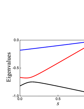
(a)

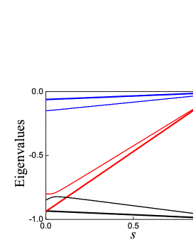
(b)

Figure 2: (Color online) Eigenvalue spectrum of the adiabatic Hamiltonian $H_{i}^{\prime}\left(s\right)$ of an intermediate step with $N_{i}/N_{i-1}=1/10$ vs. the parameter $s$ by setting the parameter $N_{i}/N$ at different values. ($a$) $N_{i}/N=1/30$, ($b$) the dashed thin lines represent the case $N_{i}/N=1/50$, and the solid thick lines represent the case $N_{i}/N=1/150$.

What about applying AQC for this problem using the same path as our algorithm? We set $N_{i}/N_{i-1}$ to be finite, thus the conditions of our algorithm are satisfied. Let the system evolve from the ground state of $H_{i-1}$ to that of $H_{i}$ under adiabatic Hamiltonian $H_{i}^{\prime}\left(s\right)=\left(1-s\right)H_{i-1}+sH_{i}$. We set $N_{i}/N_{i-1}=1/10$ and calculate eigenvalues of $H_{i}^{\prime}\left(s\right)$ for $1<i<m$. In Fig. 2, we draw the energy spectrum of $H_{i}^{\prime}\left(s\right)$ vs. $s$ where $0<s<1$ by setting $N_{i}/N=1/30$, $1/50$ and $1/150$, respectively. As $N_{i}/N$ becomes small, the minimum energy gap between the ground and the first excited states decreases quickly as $s\rightarrow 0$, and scales as $O(1/N^{2})$ at the asymptotic limit of $N$ (see see Appendix E). Thus the usual AQC algorithm cannot solve this problem efficiently using the path of our algorithm. The reason for this may due to the structure coefficients $N_{i}$ of the problem are used in constructing the intermediate Hamiltonians. It has been found that for adiabatic path constructed in linear interpolation of two Hamiltonians, gaps can become super-exponentially small, the time for adiabatic evolution is longer than the time required for even a classical brute force search AT ; Hastings . In see Appendix F, we summarize the performance of different algorithms for solving the structured search problems.

V Discussion

We present a quantum algorithm that solves a problem through a multi-step quantum computation process in which an unknown quantum state can be protected and reused without copying it. The runtime is proportional to the number of steps of the algorithm, provided the conditions of the algorithm are satisfied. We find a type of structured search problems can be solved efficiently by using our algorithm. Classically one has to check the items one by one to find the target item in solving these problems, the cost scales as the number of items $O(N)$. Our algorithm achieves an exponential speedup over classical algorithms in solving these problems in time that scales $O(\log N)$.

In Ref. AT , a jagged adiabatic path approach was proposed for running AQC by using a sequence of Hamiltonians as stepping stones. This approach can have the same complexity as our algorithm by using the same intermediate Hamiltonians. It requires to project out the ground state of each Hamiltonian to form an adiabatic path. In comparison, our algorithm is much simpler, it needs only one ancilla qubit, and the implementation requires only Hamiltonian simulation for which there are optimal quantum algorithms QSP ; qubitization for simulatable Hamiltonians. Our algorithm of multi-step quantum computation can be used for universal quantum computing and developing new quantum algorithms for other problems.

In the following appendix, we present the error analysis of the algorithm in the main text in Appendix A. In Appendix B, we apply our algorithm for solving the Deutsch-Jozsa problem; in Appendix C, we apply our algorithm for solving the unstructured search problem; in Appendix D, we apply Grover’s algorithm for solving the search problem with a special structure by using a number of different oracles; in Appendix E, we study the application of the quantum adiabatic algorithm for solving the search problem with a special structure via the same evolution path as our algorithm; and in Appendix F, we summarize the performance of different algorithms for solving the search problem with a special structure.

Appendix A Error analysis

In the $l$-th step of the algorithm, we are given Hamiltonians $H_{l}$, $H_{l-1}$ and its ground state $|\varphi_{0}^{\left(l-1\right)}\rangle$ and the ground state eigenvalue $E_{0}^{\left(l-1\right)}$ that have been obtained from the previous $(l-1)$-th step, the goal is to prepare the ground state $|\varphi_{0}^{\left(l\right)}\rangle$ and obtain its corresponding eigenvalue $E_{0}^{\left(l\right)}$ of the Hamiltonian $H_{l}$. This can be achieved via the quantum resonant transitions (QRT) method by optimizing the algorithm in Ref. whf0 ; whf2 . The algorithm requires $\left(n+1\right)$ qubits with one probe qubit and an $n$-qubit quantum register $R$ representing a Hamiltonian of dimension $N=2^{n}$. The Hamiltonian for the $l$-th step of the algorithm is constructed as

$$H^{\left(l\right)}=-\frac{1}{2}\omega\sigma_{z}\otimes I_{N}+H_{R}^{\left(l\right)}+c\sigma_{x}\otimes I_{N},$$ (8)

where

$$H_{R}^{\left(l\right)}=\alpha_{l}|1\rangle\langle 1|\otimes H_{l-1}+|0\rangle\langle 0|\otimes H_{l}\mathbf{,}\text{\ }l=1,2,\cdots,m,$$ (9)

and $I_{N}$ is the $N$-dimensional identity operator, $\sigma_{x,\text{ }z}$ are the Pauli matrices. The first term in Eq. (A$1$) is the Hamiltonian of the probe qubit, the second term describes the interaction between the probe qubit and the register $R$, and the third term is a perturbation, where $c\ll 1$ and $\alpha_{l}$ is an adjustable parameter. The Hamiltonians $H_{l-1}$ and $H_{l}$ have eigenstates $H_{l-1}|\varphi_{j}^{\left(l-1\right)}\rangle=E_{j}^{\left(l-1\right)}|\varphi_{j}^{\left(l-1\right)}\rangle$, and $H_{l}|\varphi_{j}^{\left(l\right)}\rangle=E_{j}^{\left(l\right)}|\varphi_{j}^{\left(l\right)}\rangle$, respectively, where $j=0,\cdots,N-1$.

For some problems, e.g. the search problem with a special structure in the main text where $N_{j}$ are known, the intermediate Hamiltonians can be solved analytically, we can calculate the ground state eigenvalues of the intermediate Hamiltonians and the overlaps $d_{0}^{(l)}$ between ground states of $H_{l-1}$ and $H_{l}$, and set the optimal runtime $t_{\text{opt}}=\pi/(2cd_{0}^{(l)})$ for running the algorithm to evolve the system to the ground state of $H_{l}$. For these problems, the optimal runtime $t_{\text{opt}}$ and the eigenvalues $E_{0}^{\left(l\right)}$ are known exactly.

In general, the intermediate Hamiltonians may not be solved analytically. We need to find accurate value of the ground state eigenvalue of the Hamiltonian $H_{l}$ to adjust the parameters to satisfy the resonant transition condition in QRT, while we do not need to know accurate value of the overlaps $d_{0}^{(l)}$. The reason for this is as follows: if we know the overlaps $d_{0}^{(l)}$, we can set the optimal runtime $t_{\text{opt}}=\pi/(2cd_{0}^{(l)})$, then the resonant transition probability reaches its maximum as the condition for QRT is satisfied, the algorithm will be more efficient. Without knowing the exact value of $d_{0}^{(l)}$, we can set an estimated runtime $t$ to run the QRT method, in this case, the resonant transition probability is approximately $p_{0}^{(l)}=\sin^{2}\left(ctd_{0}^{(l)}\right)$. Most likely it does not reach its maximum. In this case we just repeat the procedures of the algorithm for a few times until the resonant transition occurs. The number of times the procedures have to be repeated is proportional to $1/p_{0}^{(l)}$. This will add extra finite cost of the algorithm.

Now we describe how to obtain the ground state eigenvalue $E_{0}^{\left(l\right)}$ accurately. In order to obtain the accurate $E_{0}^{\left(l\right)}$, we need to locate the accurate resonant transition frequency that corresponds to the maximum transition probability of the probe qubit for a given estimated runtime $t$. In searching for the resonant transition frequency, we discritize an estimated probe frequency range into a number of grids to form a frequency set. The width of the grids should be smaller than the width of the transition peaks of the probe qubit, which is given by $\max\left[cd_{0}^{(l)},1/t\right]$ whf1 . We set the probe qubit in a frequency, and run the procedures of the algorithm for a number of times. If a resonant transition is not observed, we try the next frequency and run the algorithm. The cost of this process is proportional to the number of frequency points in the discretized frequency set. Here we note that in general, the transition frequency $\omega$ of a qubit in a digital quantum computer is fixed. While in our algorithm, variation of the transition frequency $\omega$ of the probe qubit can be realized equivalently by adjusting the parameter $\alpha_{l}$, e.g. for the probe qubit frequency to be varied in frequency range $\left[\omega_{\min},\omega_{\max}\right]$, this can be equivalently realized by setting the parameter $\alpha_{l}$ in a range $\left[\alpha_{l\max},\alpha_{l\min}\right]$, where $E_{0}^{\left(l\right)}-\alpha_{l\max}E_{0}^{\left(l-1\right)}=\omega_{\min}$, and $E_{0}^{\left(l\right)}-\alpha_{l\min}E_{0}^{\left(l-1\right)}=\omega_{\max}$.

In order to obtain the accurate value of $E_{0}^{\left(l\right)}$, we need to locate the accurate resonant transition frequency corresponding to the maximum transition probability of the probe qubit for a given estimated runtime $t$. We may not obtain it in one step, most likely we have to try a number of times back and forth around the accurate resonant transition frequency. Suppose we are trying the frequencies of the probe qubit from small to large values, if we pass the accurate value, we need to go back and try another frequency. This can be done by modifying the Hamiltonian in Eq. (A$2$) to switch the adjacent Hamiltonians $H_{l-1}$ and $H_{l}$: $H_{R}^{\prime\left(l\right)}=\alpha_{l}|1\rangle\langle 1|\otimes H_{l}+|0\rangle\langle 0|\otimes H_{l-1}$, and run the procedures of the algorithm to drive the system back to state $|\varphi_{0}^{\left(l-1\right)}\rangle$. We can repeat this procedure while varying the frequency of the probe qubit near the resonant transition frequency to obtain accurate value of $E_{0}^{\left(l\right)}$. The cost is proportional to the number of times of the procedures needs to be repeated, which scales as $O(1/\epsilon^{2})$ where $\epsilon$ denotes the accuracy of $E_{0}^{\left(l\right)}$. And the cost for the case when there is a deviation $\epsilon$ of the probe frequency from the resonant transition frequency is analyzed at the end of this section.

In the following, we estimate errors introduced when running the algorithm by using the accurate value of $E_{0}^{\left(l\right)}$ and the optimal runtime $t$. Let

$$H_{0}^{\left(l\right)}=-\frac{1}{2}\omega\sigma_{z}\otimes I_{N}+H_{R}^{\left(l\right)},$$ (10)

then the algorithm Hamiltonian $H^{\left(l\right)}$ can be written as $H^{\left(l\right)}=H_{0}^{\left(l\right)}+c\sigma_{x}\otimes I_{N}$. The Hamiltonian $H_{0}^{\left(l\right)}$ is the unperturbed term and has eigenstates

$$H_{0}^{\left(l\right)}|1\rangle|\varphi_{j}^{\left(l-1\right)}\rangle=\left(\frac{\omega}{2}\!+\!\alpha_{l}E_{j}^{(l-1)}\right)|1\rangle|\varphi_{j}^{\left(l-1\right)}\rangle,$$ (11)

and

$$H_{0}^{\left(l\right)}|0\rangle|\varphi_{j}^{\left(l\right)}\rangle=\left(\frac{-\omega}{2}\!+\!E_{j}^{(l)}\right)|0\rangle|\varphi_{j}^{\left(l\right)}\rangle,$$ (12)

where $j=0,1,\cdots,N-1$. In the $l$-th step of the algorithm, the system is initialized in state $|1\rangle|\varphi_{0}^{\left(l-1\right)}\rangle$. When the resonant transition condition $E_{0}^{\left(l\right)}-\alpha_{l}E_{0}^{\left(l-1\right)}=\omega$ is satisfied, the system is transferred to state $|0\rangle|\varphi_{j}^{\left(l\right)}\rangle$ through QRT. Errors in the algorithm are introduced by excitations from the initial state to the excited states $|0\rangle|\varphi_{j}^{\left(l\right)}\rangle$ ($j=1,\cdots,N-1$) of the unperturbed Hamiltonian $H_{0}^{\left(l\right)}$ induced by the perturbation term.

For a system consists of a probe qubit coupled to a two-level system described by the Hamiltonian in Eq. (A$1$), the maximum transition probability from the ground state to the excited state of the two-level system becomes higher as the transition frequency between the two-level system gets closer to the frequency of the probe qubit. Based on this observation, the upper bound of the error of the algorithm, that is, the upper bound of the transition probability from the initial state to the excited states, can be obtained by ($i$) assuming all the excited states are degenerate at the first excited state of the unperturbed Hamiltonian $H_{0}^{\left(l\right)}$, and ($ii$) without considering competition of the transition from the initial state to the target state $|0\rangle|\varphi_{j}^{\left(l\right)}\rangle$ through QRT, which is the ground state of the unperturbed Hamiltonian $H_{0}^{\left(l\right)}$. With the above analysis, the upper bound of the error in the $l$-th step of the algorithm is the probability of the system being transferred from the initial state to the state $|0\rangle|\varphi_{1}^{\left(l\right)}\rangle$ described by the algorithm Hamiltonian in basis of $\left\{|1\rangle|\varphi_{0}^{\left(l-1\right)}\rangle,|0\rangle|\varphi_{1}^{\left(l\right)}\rangle\right\}$ as:

$${H_{err}^{(l)}=}\left(\begin{array}[]{cc}-\frac{1}{2}\omega+E_{0}^{(l)}&c\sqrt{1-\left|{d_{0}^{(l)}}\right|^{2}}\\ c\sqrt{1-\left|{d_{0}^{(l)}}\right|^{2}}&-\frac{1}{2}\omega+E_{1}^{(l)}\end{array}\right),$$ (13)

here we have denoted $d_{j0}=\langle\varphi_{j}^{(l)}|\varphi_{0}^{(l-1)}\rangle$ and $d_{0}^{(l)}=d_{00}>0$. The transition probability from the initial state $|1\rangle|\varphi_{0}^{\left(l-1\right)}\rangle$ to the state $|0\rangle|\varphi_{1}^{\left(l\right)}\rangle$ is:

$$\frac{4c^{2}\left[1-\left(d_{0}^{(l)}\right)^{2}\right]}{4c^{2}\left[1-\left(d_{0}^{(l)}\right)^{2}\right]+\left[E_{1}^{(l)}-\!\alpha_{l}E_{0}^{(l-1)}-\omega\right]^{2}}\sin^{2}\left[\frac{t}{2}\sqrt{4c^{2}\left[1-\left(d_{0}^{(l)}\right)^{2}\right]+\left[E_{1}^{(l)}-\!\alpha_{l}E_{0}^{(l-1)}-\omega\right]^{2}}\right],$$ (14)

by using the Rabi’s formula cohen . Therefore considering the resonant transition condition $E_{0}^{\left(l\right)}-\alpha_{l}E_{0}^{\left(l-1\right)}=\omega$, the upper bound of the transition probabilities from the initial state to the excited states $|0\rangle|\varphi_{j}^{\left(l\right)}\rangle$ ($j=1,\cdots,N-1$) can be estimated as

$$\sum_{j=1}^{N-1}p_{j}\leq\frac{4c^{2}\left[1-\left(d_{0}^{(l)}\right)^{2}\right]}{4c^{2}\left[1-\left(d_{0}^{(l)}\right)^{2}\right]+\left[E_{1}^{(l)}-\!\alpha_{l}E_{0}^{(l-1)}-\omega\right]^{2}}<\frac{4c^{2}\left[1-\left(d_{0}^{(l)}\right)^{2}\right]}{\left[E_{1}^{(l)}-\!E_{0}^{(l)}\right]^{2}}.$$ (15)

We obtain the upper bound of the error introduced by transition from the initial state to the excited states of the target Hamiltonian of the ${l}$-th step $H_{l}$.

We denote $a_{l}^{2}=\frac{4\left[1-\left(d_{0}^{(l)}\right)^{2}\right]}{\left[E_{1}^{(l)}-\!E_{0}^{(l)}\right]^{2}}$. If the energy gap $E_{1}^{(l)}-E_{0}^{(l)}\gg c$ is not exponentially small, i.e., bounded by a polynomial function of the problem size, then $a_{l}$ is a finite number and the error in the $l$-th step is bounded by $a_{l}^{2}c^{2}$. Considering errors accumulated in all steps of the algorithm, the success probability of the algorithm for obtaining the ground state of the problem Hamiltonian satisfies

$$P_{\text{succ}}\geqslant\prod_{l=1}^{m}\left(1-a_{l}^{2}c^{2}\right)\geqslant\left[1-\left(a_{\max}c\right)^{2}\right]^{m},$$ (16)

where $a_{\max}$ is the maximum value of $a_{l}$ for $l=1,\ldots,m$. The coefficient $c$ can be set such that $a_{\max}c<1/\sqrt{m}$, then $P_{\text{succ}}>1/e$ in the asymptotic limit of $m$.

Now we consider the cost when there is deviation $\epsilon$ of the probe frequency from the resonant transition frequency. By ignoring the off-resonant transition, the transition probability from the state $|1\rangle|\varphi_{0}^{\left(l-1\right)}\rangle$ to $|0\rangle|\varphi_{0}^{\left(l\right)}\rangle$ is $\sin^{2}\left(\frac{\Omega_{0}}{2}t\right)\frac{\left(2cd_{0}^{(l)}\right)^{2}}{\Omega_{0}^{2}}$ where $\Omega_{0}=\sqrt{\left(2cd_{0}^{(l)}\right)^{2}+\epsilon^{2}}$. The transition probability is finite if $\epsilon<2cd_{0}^{(l)}$. The number of times that this procedure needs to be repeated scales as $O(1/\epsilon^{2})$, and the cost is finite as long as $d_{0}^{(l)}$ and $c$ are not exponentially small.

Appendix B Application of the algorithm for the Deutsch-Jozsa problem

In the context of our algorithm, the Deutsch-Jozsa problem is described as: given a function $f:\left\{0,1\right\}^{n}\longmapsto\left\{0,-1\right\}$ which is either constant for all values of $x$ or balanced, i.e., $f\left(x\right)=0$ on half the inputs and $f\left(x\right)=-1$ on the other half. The Deutsch-Jozsa problem is to determine which type the function is. Classically, the problem requires ($2^{n-1}+1$) queries of the function $f$ in the worst case. The Deutsch-Jozsa algorithm solves this problem in a single query of $f$.

Our algorithm can also be applied for solving this problem efficiently. In the case where $f$ is balanced, the total number of $N=2^{n}$ states can be divided into two sets by using an oracle $f$. The set with eigenvalue $-1$ has $N_{1}=2^{n-1}$ items, thus the ratio $N_{1}/N=1/2$. To apply our algorithm, we set the initial state of the problem to be $|\psi_{0}\rangle=\frac{1}{\sqrt{N}}\sum_{j=0}^{N-1}|j\rangle$, the overlap between the initial state and the target state $|\psi_{1}\rangle=\frac{1}{\sqrt{N_{1}}}\sum_{x,f(x)=-1}|x\rangle$ is $1/\sqrt{2}$, therefore our algorithm can determine whether the function is a balanced function in time $t=\pi/(\sqrt{2}c)$, when observing decay of the probe qubit with probability one. On the other hand, if the resonant transition is not observed with probability one at time $t=\pi/(\sqrt{2}c)$, we know the function is constant. In this case, if the constant is $0$, there will be no resonant transition; if the constant is $-1$, then the resonant transition probability reaches one at runtime $t=\pi/(2c)$. These cases can be easily distinguished in our algorithm, therefore we can find out whether the function $f$ is constant or balanced.

Appendix C Application of the algorithm for the unstructured search problem

The unstructured search problem is to find a marked item in an unsorted database of $N$ items using an oracle that recognizes the marked item. The oracle is defined in terms of a problem Hamiltonian

$$H_{P}=-|q\rangle\langle q|,$$ (17)

where $|q\rangle$ is the marked state associated with the marked item. The initial Hamiltonian is defined as

$$H_{0}=-|\psi_{0}\rangle\langle\psi_{0}|,$$ (18)

where $|\psi_{0}\rangle=\frac{1}{\sqrt{N}}\sum_{j=0}^{N-1}|j\rangle$. We can solve the unstructured search problem by using the QRT method whf0 ; whf2 directly.

We set the Hamiltonian of the algorithm as

$$H=-\frac{1}{2}\omega\sigma_{z}\otimes I_{N}+H_{R}+c\sigma_{x}\otimes I_{N},$$ (19)

where

$$H_{R}=2|1\rangle\langle 1|\otimes H_{0}+|0\rangle\langle 0|\otimes H_{P}\mathbf{,}$$ (20)

and the coupling coefficient $c\ll 1$. We set the initial state of the circuit as $|1\rangle|\psi_{0}\rangle$, which is the eigenstate of $H_{R}$ with eigenvalue $-2$. The transition frequency of the probe qubit is set as $\omega=1$, such that the resonant transition condition between states $|1\rangle|\psi_{0}\rangle$ and $|0\rangle|q\rangle$ is satisfied. The overlap between the initial state $|\psi_{0}\rangle$ and the target state $|q\rangle$ is $d_{0}=\frac{1}{\sqrt{N}}$. By applying the QRT method, the decay probability of the probe qubit is $p_{0}=\sin^{2}\left(ctd_{0}\right)$, which reaches its maximum $1$ at $t=\frac{\pi}{2cd_{0}}$. Therefore the system can evolve to the target state in runtime scales as $O(\sqrt{N})$. In the case of multiple marked items in a database, the problem Hamiltonian is defined as $H_{P}=-\sum_{q_{j}\in\Pi}|q_{j}\rangle\langle q_{j}|$, where $\Pi$ is a set of marked states associated with the marked items of size $N_{q}$. The overlap between the initial state $|\psi_{0}\rangle$ and the target state $\frac{1}{\sqrt{N_{q}}}\sum_{q_{j}\in\Pi}|q_{j}\rangle|q_{j}\rangle$ is $\sqrt{N_{q}/N}$. By applying the QRT method, the system can evolve to the target state in runtime scales as $O(\sqrt{N/N_{q}})$. In both cases, the runtime of our algorithm is the same as that of Grover’s algorithm grover and the adiabatic quantum computing (AQC) algorithm cerf ; lidar .

Appendix D Solving the search problem with a special structure via Grover’s algorithm

In the main manuscript, we have shown that the search problem with a special structure can be solved efficiently by using the QRT method in $m$ steps, where the problem can be decomposed by $m$ different oracles and $m$ scales in order of $O\left(\log N\right)$. We have also shown in the above section that by using one oracle, the unstructured search problem can be solved by the QRT method with the same efficiency as that of the Grover’s algorithm. Then a natural question is: can the structured search problem be solved efficiently by using the Grover’s algorithm with $m$ different oracles? We analyze this problem as follows:

The structured search problem can be decomposed by $m$ different oracles that are defined in terms of $m$ Hamiltonians

$$H_{P_{j}}=-\sum_{q_{j}\in\Pi_{j}}|q_{j}\rangle\langle q_{j}|,$$ (21)

and $H_{P_{m}}=H_{P}=-|q\rangle\langle q|$, where $|q\rangle$ is the marked state associated with the marked item, and the set $\Pi_{m}$ only contains the target state $|q\rangle$, and $\Pi_{1}\supset\cdots\supset\Pi_{m-1}\supset\Pi_{m}$, with size $N_{1}$, $\cdots$, $N_{m-1}$, $N_{m}=1$, respectively. Here $N_{j}$ are known and $N_{j}/N_{j-1}$ ($j=1,2,\cdots,m$) are not exponentially small. The corresponding oracles are $O_{1}$, $\cdots$, $O_{m}$, respectively. The initial Hamiltonian is defined as $H_{0}=-|\psi_{0}\rangle\langle\psi_{0}|$, where $|\psi_{0}\rangle=\frac{1}{\sqrt{N}}\sum_{k=0}^{N-1}|k\rangle$.

Since $N_{j}$ are already known, the fixed-point search can be performed by using Grover’s algorithm. In the first iteration, the Grover operator is constructed as:

$$G_{1}=\left(2|\psi_{0}\rangle\langle\psi_{0}|-I\right)O_{1}=R_{1}O_{1},$$ (22)

by applying $G_{1}$ for $O\left(\sqrt{N/N_{1}}\right)$ times, we can obtain state $|\psi_{1}\rangle=\frac{1}{\sqrt{N_{1}}}\sum_{q_{1}\in\Pi_{1}}|q_{1}\rangle$. The oracle $O_{1}$ is queried for $O\left(\sqrt{N/N_{1}}\right)$ times. The Grover operator of the second iteration is:

$$G_{2}=\left(2|\psi_{1}\rangle\langle\psi_{1}|-I\right)O_{2}=R_{2}O_{2},$$ (23)

by applying $G_{2}$ for $O\left(\sqrt{N_{1}/N_{2}}\right)$ times, we obtain state $|\psi_{2}\rangle=\frac{1}{\sqrt{N_{2}}}\sum_{q_{2}\in\Pi_{2}}|q_{2}\rangle$. This iteration requires the oracle $O_{1}$ to be queried for $\sqrt{N/N_{1}}\times\sqrt{N_{1}/N_{2}}=\sqrt{N/N_{2}}$ times and the oracle $O_{2}$ for $\sqrt{N_{1}/N_{2}}$ times. By repeating this procedure after $m$ iterations, the target state $|q\rangle$ is obtained. The oracle $O_{1}$ is queried for $O\left(\sqrt{N}\right)$ times, and the oracle $O_{2}$ for $O\left(\sqrt{N_{1}}\right)$ times, …, etc.

Based on the above analysis, we can see that Grover’s algorithm cannot achieve the same efficiency as our algorithm in solving the structured search problem by using $m$ oracles. We can see that in applying Grover’s algorithm for solving the problem, only one quantum computation process is applied. While in our algorithm, we apply a multi-step quantum computation process. In our algorithm, an oracle is used in only one step of the algorithm to obtain the desired state of the step. By using techniques of QRT, post-selection and measurement on the probe qubit, the desired state of the step is obtained deterministically. The desired state is protected through quantum entanglement and can be used repeatedly for the next step of the algorithm. These properties of the algorithm make it achieve better efficiency than that of Grover’s algorithm in solving the structured search problem.

Appendix E Solving the search problem with a special structure via quantum adiabatic evolution

In the unstructured search problem, the problem Hamiltonian is $H_{P}=-|q\rangle\langle q|$, where $|q\rangle$ is the marked state associated with the marked item, and the initial Hamiltonian is given by $H_{0}=-|\psi_{0}\rangle\langle\psi_{0}|$, where $|\psi_{0}\rangle=\frac{1}{\sqrt{N}}\sum_{j=0}^{N-1}|j\rangle$. The initial Hamiltonian $H_{0}$ has two energy levels: $-1$ with corresponding eigenstate $|\psi_{0}\rangle$ and $0$ with $(N-1)$ eigenstates $|\psi_{0}^{\bot}\rangle$ that are orthogonal to $|\psi_{0}\rangle$. For a search problem with a special structure that it can be decomposed by using a number of different oracles and allows us to construct a sequence of intermediate Hamiltonians

$$H_{j}=\frac{N_{j}}{N}H_{0}+\left(1-\frac{N_{j}}{N}\right)H_{P_{j}},\text{ \ }j=1,2,\cdots,m-1,$$ (24)

and

$$H_{P_{j}}=-\sum_{q_{j}\in\Pi_{j}}|q_{j}\rangle\langle q_{j}|,$$ (25)

where $\Pi_{1}\supset\cdots\supset\Pi_{m-1}$, the sizes of $\Pi_{1}$, $\cdots$, $\Pi_{m-1}$ are $N_{1}$, $\cdots$, $N_{m-1}$, respectively, and $N_{1}>\cdots>N_{m-1}$, and inserted between the initial Hamiltonian $H_{0}$ and the problem Hamiltonian $H_{P}$ (see Fig. 3). Let $H_{m}=H_{P}$ and the set $\Pi_{m}$ only contains the target state $|q\rangle$ with size $N_{m}=1$, and $\Pi_{m-1}\supset\Pi_{m}$. We demonstrate in the main text that as long as the ratio $N_{j}/N_{j-1}$ ($j=1,2,\cdots,m$) are not exponentially small, the problem can be solved efficiently by our algorithm step by step through the evolution path $H_{0}\rightarrow H_{1}\rightarrow\cdots\rightarrow H_{m}=H_{P}$ as constructed above. We start from the ground state $|\varphi_{0}^{(0)}\rangle$ of $H_{0}$, and evolve it through ground states of the intermediate Hamiltonians sequentially using the QRT method, finally reach the ground state $|\varphi_{0}^{(m)}\rangle$ of $H_{P}$ in $m$ steps. An interesting question is: will this problem be solved efficiently through quantum adiabatic evolution using the same evolution path of our algorithm? In the following, we study the quantum adiabatic evolution from the ground state of the initial Hamiltonian $H_{0}$ to that of the problem Hamiltonian $H_{P}$ through the evolution path of our algorithm step by step. In each step, the system is evolved adiabatically from the ground state of the Hamiltonian $H_{j-1}$ to that of its next neighbor $H_{j}$, finally reach the ground state of the problem Hamiltonian $H_{P}$. Note that here we apply the usual quantum adiabatic evolution Hamiltonian $H_{j}^{\prime}\left(s\right)=\left(1-s\right)H_{j-1}+sH_{j}$, $s\in\left[0,1\right]$ in each step.

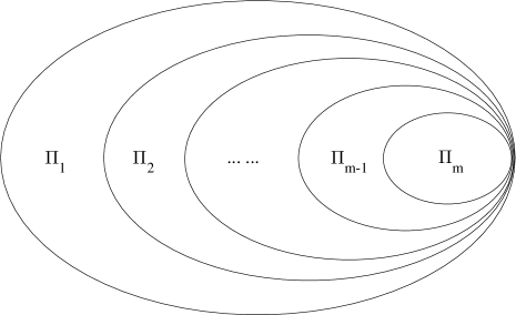
Figure 3: The index sets $\Pi_{1}\supset\Pi_{2}\supset\cdots\supset\Pi_{m}$.

E.1 Eigen-problem of the intermediate Hamiltonians

First we solve the eigen-problem of an intermediate Hamiltonian $H_{j}$. Define

$$|\psi_{0}\rangle=\frac{1}{\sqrt{N}}\sum_{j=0}^{N-1}|j\rangle=\frac{1}{\sqrt{N}}\sum_{q_{j}\in\Pi_{j}}|q_{j}\rangle+\sqrt{\frac{N-N_{j}}{N}}|q_{j}^{\bot}\rangle.$$ (26)

where

$$|q_{j}^{\bot}\rangle=\frac{1}{\sqrt{N-N_{j}}}\sum_{k\notin\Pi_{j}}|k\rangle.$$ (27)

Then in the basis $\left(\left\{|q_{j}\rangle\right\}_{q_{j}\in\Pi_{j}}\text{, }|q_{j}^{\bot}\rangle\right)$ we have

$$H\!_{0}\!\! = -|\psi_{0}\rangle\langle\psi_{0}|$$ (32)

$$= -\!\!\left(\!\!\begin{array}[]{cccc}\frac{1}{N}&\cdots&\frac{1}{N}&\frac{\sqrt{\!N\!-\!N_{j}}}{N}\\ \vdots&\ddots&\vdots&\vdots\\ \frac{1}{N}&\cdots&\frac{1}{N}&\frac{\sqrt{N\!-\!N_{j}}}{N}\\ \frac{\sqrt{\!N\!-\!N_{j}}}{N}&\cdots&\frac{\sqrt{\!N\!-\!N_{j}}}{N}&\frac{\!N\!-\!N_{j}\!}{N}\!\end{array}\!\!\right),$$

and

$$H_{P_{j}} = -\sum_{q_{j}\in\Pi_{j}}|q_{j}\rangle\langle q_{j}|$$ (37)

$$= -\!\!\left(\!\!\begin{array}[]{cccc}1&\cdots&0&0\\ \vdots&\ddots&\vdots&\vdots\\ 0&\cdots&1&0\\ 0&\cdots&0&0\end{array}\!\!\right).$$

Then

$$H_{j} = \frac{N_{j}}{N}H_{0}+\left(1-\frac{N_{j}}{N}\right)H_{P_{j}}$$ (43)

$$= -\!\!\left(\!\!\begin{array}[]{ccccc}\frac{N_{j}}{N^{2}}+1-\frac{N_{j}}{N}&\frac{N_{j}}{N^{2}}&\cdots&\frac{N_{j}}{N^{2}}&\frac{N_{j}\sqrt{\!N\!-\!N_{j}}}{N^{2}}\\ \frac{N_{j}}{N^{2}}&\frac{N_{j}}{N^{2}}+1-\frac{N_{j}}{N}&\cdots&\vdots&\vdots\\ \vdots&\vdots&\ddots&&\\ \frac{N_{j}}{N^{2}}&\frac{N_{j}}{N^{2}}&\cdots&\frac{N_{j}}{N^{2}}+1-\frac{N_{j}}{N}&\frac{N_{j}\sqrt{N\!-\!N_{j}}}{N^{2}}\\ \frac{N_{j}\sqrt{\!N\!-\!N_{j}}}{N^{2}}&\frac{N_{j}\sqrt{\!N\!-\!N_{j}}}{N^{2}}&\cdots&\frac{N_{j}\sqrt{\!N\!-\!N_{j}}}{N^{2}}&\frac{N_{j}\left(N\!-\!N_{j}\right)\!\!}{N^{2}}\end{array}\!\!\right).$$

Let

$$\mathbf{e}=\left(\begin{array}[]{c}1\\ \vdots\\ 1\\ 1\end{array}\right)_{(N_{j}+1)\times 1},\qquad\mathbf{e}_{n}=\left(\begin{array}[]{c}0\\ \vdots\\ 0\\ 1\end{array}\right)_{(N_{j}+1)\times 1},$$ (44)

then $H_{0}$ can be written as

$$H_{0} = -\left(\frac{1}{\sqrt{N}}\mathbf{e}+\frac{\sqrt{N-N_{j}}-1}{\sqrt{N}}\mathbf{e}_{n}\right)\left(\frac{1}{\sqrt{N}}\mathbf{e}+\frac{\sqrt{N-N_{j}}-1}{\sqrt{N}}\mathbf{e}_{n}\right)^{T}$$ (45)

$$= -\frac{1}{N}\mathbf{e}\mathbf{e}^{T}-\frac{\sqrt{N-N_{j}}-1}{N}\left(\mathbf{e}\mathbf{e}_{n}^{T}+\mathbf{e}_{n}\mathbf{e}^{T}\right)-\frac{\left(\sqrt{\!N\!-\!N_{j}}-1\right)^{2}}{N}\mathbf{e}_{n}\mathbf{e}_{n}^{T},$$

and

$$H_{P_{j}}=-\left(I_{n}-\mathbf{e}_{n}\mathbf{e}_{n}^{T}\right),$$ (46)

where $I_{n}$ is the $(N_{j}+1)$-dimensional identity operator.

Thus

$$H_{j} = \frac{N_{j}}{N}H_{0}+\left(1-\frac{N_{j}}{N}\right)H_{P_{j}}$$ (47)

$$= \!-\frac{N_{j}}{N}\!\left[\!\frac{1}{N}\mathbf{e}\mathbf{e}^{T}\!+\!\frac{\sqrt{N\!-\!N_{j}}\!-\!1}{N}\left(\!\mathbf{e}\mathbf{e}_{n}^{T}\!+\!\mathbf{e}_{n}\mathbf{e}^{T}\!\right)\!+\!\frac{\left(\!\sqrt{\!N\!-\!N_{j}}\!-\!1\!\right)^{2}}{N}\mathbf{e}_{n}\mathbf{e}_{n}^{T}\!\right]\!\!-\!\!\left(\!1\!-\!\frac{N_{j}}{N}\!\right)\left(\!I_{n}\!-\!\mathbf{e}_{n}\mathbf{e}_{n}^{T}\!\right)$$

$$= -\frac{N_{j}}{N^{2}}\mathbf{e}\mathbf{e}^{T}\!-\!\frac{N_{j}\left(\!\sqrt{N-N_{j}}\!-\!1\!\right)}{N^{2}}\left(\mathbf{e}\mathbf{e}_{n}^{T}\!+\!\mathbf{e}_{n}\mathbf{e}^{T}\right)\!+\!\left[\!\left(\!1\!-\!\frac{N_{j}}{N}\!\right)\!-\!\frac{N_{j}\left(\!\sqrt{\!N\!-\!N_{j}}\!-\!1\!\right)^{2}}{N^{2}}\!\right]\mathbf{e}_{n}\mathbf{e}_{n}^{T}$$

$$-\left(1-\frac{N_{j}}{N}\right)I_{n}$$

$$\equiv \alpha\mathbf{e}\mathbf{e}^{T}+\beta\left(\mathbf{e}\mathbf{e}_{n}^{T}+\mathbf{e}_{n}\mathbf{e}^{T}\right)+\left(\gamma-2\beta\right)\mathbf{e}_{n}\mathbf{e}_{n}^{T}-\left(1-\frac{N_{j}}{N}\right)I_{n},$$

where $\alpha=-\frac{N_{j}}{N^{2}}$, $\beta=-\frac{N_{j}\left(\sqrt{N-N_{j}}-1\right)}{N^{2}}$, $\gamma=2\beta+1-\frac{N_{j}}{N}-\frac{N_{j}\left(\sqrt{\!N\!-\!N_{j}}-1\right)^{2}}{N^{2}}$. Please note that, with a bit abuse of notation, in the following we will reuse the notations $\mathbf{e}$, $\mathbf{e}_{n}$, $\alpha$, $\beta$ and $\gamma$, and their dimensions and values can be determined easily from the context.

Define $\tilde{\mathbf{e}}$ as the $N_{j}\times 1$ vector of all ones, and we can rewrite $H_{j}$ as

$$H_{j}=\alpha\mathbf{e}\mathbf{e}^{T}\!+\!\left(\begin{array}[]{cc}\mathbf{0}_{N_{j}}&\beta\tilde{\mathbf{e}}\\ \beta\tilde{\mathbf{e}}^{T}&\gamma\end{array}\right)-\left(1-\frac{N_{j}}{N}\right)I_{n}\equiv\alpha\mathbf{e}\mathbf{e}^{T}+G-\left(1-\frac{N_{j}}{N}\right)I_{n}.$$

($i$) Define the vector space $V=\left\{\mathbf{e},\mathbf{e}_{n}\right\}$ of dimension $2$. Then from Eq. (47), $\forall x\in V^{\perp}$, we have $H_{j}x=-\left(1-\frac{N_{j}}{N}\right)x$, therefore the eigenvalues are $-\left(1-\frac{N_{j}}{N}\right)$, corresponding to $N_{j}-1$ eigenvectors.

($ii$) The vector space of $V$ can be spanned by vectors

$$W=\left[\frac{1}{\sqrt{N_{j}}}\left(\begin{array}[]{c}1\\ \vdots\\ 1\\ 0\end{array}\right),\left(\begin{array}[]{c}0\\ \vdots\\ 0\\ 1\end{array}\right)\right].$$

It is easy to check that

$$W^{T}GW=\left(\begin{array}[]{cc}0&\beta\sqrt{N_{j}}\\ \beta\sqrt{N_{j}}&\gamma\end{array}\right),$$

and

$$W^{T}\mathbf{e}=\left(\begin{array}[]{c}\sqrt{N_{j}}\\ 1\end{array}\right).$$

Then we can verify that

$$W^{T}H_{j}W = \alpha W^{T}\mathbf{e}\mathbf{e}^{T}W+W^{T}GW-\left(1-\frac{N_{j}}{N}\right)I$$ (50)

$$= \left(\begin{array}[]{cc}\alpha N_{j}&\left(\alpha+\beta\right)\sqrt{N_{j}}\\ \left(\alpha+\beta\right)\sqrt{N_{j}}&\alpha+\gamma\end{array}\right)-\left(1-\frac{N_{j}}{N}\right)I.$$

Solving the eigen-problem of the above matrix, we can obtain the eigenvalues:

$$\lambda_{1,2}\! = \frac{1}{2}\left(\alpha N_{j}\!+\!\alpha\!+\!\gamma\right)\pm\frac{1}{2}\sqrt{(\alpha N_{j}\!+\!\alpha\!+\!\gamma)^{2}\!+\!4(\alpha\!+\!\beta)^{2}N_{j}\!-\!4\alpha N_{j}(\alpha\!+\!\gamma)}\!-\!\left(1\!-\!\frac{N_{j}}{N}\right)$$ (51)

$$= -\frac{1}{2}\pm\frac{1}{2}\sqrt{1-4\frac{N_{j}}{N}+8\left(\frac{N_{j}}{N}\right)^{2}-4\left(\frac{N_{j}}{N}\right)^{3}}.$$

Besides these $N_{j}+1$ eigenvalues above, there are also $N-(N_{j}+1)$ degenerate eigenstates with eigenvalue $0$, and they are orthogonal to both the vector space $V=\left\{e,e_{n}\right\}$ and the vector space $V^{\perp}$ of dimension $N_{j}-1$.

E.2 Quantum adiabatic evolution in the first step

In the first step, the system evolves adiabatically from the ground state $|\psi_{0}\rangle$ of $H_{0}$ to the ground state of $H_{1}=\frac{N_{1}}{N}H_{0}+\left(1-\frac{N_{1}}{N}\right)H_{P_{1}}$. Define

$$|\psi_{0}\rangle=\frac{1}{\sqrt{N}}\sum_{j=0}^{N-1}|j\rangle=\frac{1}{\sqrt{N}}\sum_{q_{1}\in\Pi_{1}}|q_{1}\rangle+\sqrt{\frac{N-N_{1}}{N}}|q_{1}^{\bot}\rangle.$$ (52)

where

$$|q_{1}^{\bot}\rangle=\frac{1}{\sqrt{N-N_{1}}}\sum_{k\notin\Pi_{1}}|k\rangle,$$ (53)

Then in the basis $\left(\left\{|q_{1}\rangle\right\}_{q_{1}\in\Pi_{1}}\text{, }|q_{1}^{\bot}\rangle\right)$ we have

$$H\!_{0}\!\! = -|\psi_{0}\rangle\langle\psi_{0}|$$ (58)

$$= -\!\!\left(\!\!\begin{array}[]{cccc}\frac{1}{N}&\cdots&\frac{1}{N}&\frac{\sqrt{\!N\!-\!N_{1}}}{N}\\ \vdots&\ddots&\vdots&\vdots\\ \frac{1}{N}&\cdots&\frac{1}{N}&\frac{\sqrt{N\!-\!N_{1}}}{N}\\ \frac{\sqrt{\!N\!-\!N_{1}}}{N}&\cdots&\frac{\sqrt{\!N\!-\!N_{1}}}{N}&\frac{\!N\!-\!N_{1}\!}{N}\!\end{array}\!\!\right),$$

and

$$H_{P_{1}} = -\sum_{q_{1}\in\Pi_{1}}|q_{1}\rangle\langle q_{1}|$$ (63)

$$= -\!\!\left(\!\!\begin{array}[]{cccc}1&\cdots&0&0\\ \vdots&\ddots&\vdots&\vdots\\ 0&\cdots&1&0\\ 0&\cdots&0&0\end{array}\!\!\right).$$

Then

$$H_{1} = \frac{N_{1}}{N}H_{0}+\left(1-\frac{N_{1}}{N}\right)H_{P_{1}}$$ (68)

$$= -\!\!\left(\!\!\begin{array}[]{cccc}\frac{N_{1}}{N^{2}}+1-\frac{N_{1}}{N}&\cdots&\frac{N_{1}}{N^{2}}&\frac{N_{1}\sqrt{\!N\!-\!N_{1}}}{N^{2}}\\ \vdots&\ddots&\vdots&\vdots\\ \frac{N_{1}}{N^{2}}&\cdots&\frac{N_{1}}{N^{2}}+1-\frac{N_{1}}{N}&\frac{N_{1}\sqrt{N\!-\!N_{1}}}{N^{2}}\\ \frac{N_{1}\sqrt{\!N\!-\!N_{1}}}{N^{2}}&\cdots&\frac{N_{1}\sqrt{\!N\!-\!N_{1}}}{N^{2}}&\frac{N_{1}(\!N\!-\!N_{1}\!)}{N^{2}}\end{array}\!\!\right).$$

The adiabatic evolution Hamiltonian from $H_{0}$ to $H_{1}$ is defined as follows:

$$H\left(s\right) = \left(1-s\right)H_{0}+sH_{1}$$ (77)

$$= \!-(\!1\!-\!s\!)\!\!\left(\!\!\begin{array}[]{cccc}\frac{1}{N}&\cdots&\frac{1}{N}&\frac{\sqrt{\!N\!-\!N_{1}}}{N}\\ \vdots&\ddots&\vdots&\vdots\\ \frac{1}{N}&\cdots&\frac{1}{N}&\frac{\sqrt{N\!-\!N_{1}}}{N}\\ \frac{\sqrt{\!N\!-\!N_{1}}}{N}&\cdots&\frac{\sqrt{\!N\!-\!N_{1}}}{N}&\frac{\!N\!-\!N_{1}\!}{N}\!\end{array}\!\!\right)\!\!-\!\!s\!\!\left(\!\!\begin{array}[]{cccc}\frac{N_{1}}{N^{2}}\!\!+\!\!1\!\!-\!\!\frac{N_{1}}{N}&\cdots&\frac{N_{1}}{N^{2}}&\frac{N_{1}\sqrt{\!N\!-\!N_{1}}}{N^{2}}\\ \vdots&\ddots&\vdots&\vdots\\ \frac{N_{1}}{N^{2}}&\cdots&\frac{N_{1}}{N^{2}}\!\!+\!\!1\!\!-\!\!1\frac{N_{1}}{N}&\frac{N_{1}\sqrt{N\!-\!N_{1}}}{N^{2}}\\ \frac{N_{1}\sqrt{\!N\!-\!N_{1}}}{N^{2}}&\cdots&\frac{N_{1}\sqrt{\!N\!-\!N_{1}}}{N^{2}}&\frac{N_{1}(\!N\!-\!N_{1}\!)}{N^{2}}\end{array}\!\!\right).$$

Let

$$\mathbf{e}=\left(\begin{array}[]{c}1\\ \vdots\\ 1\\ 1\end{array}\right)_{(N_{1}+1)\times 1},\qquad\mathbf{e}_{n}=\left(\begin{array}[]{c}0\\ \vdots\\ 0\\ 1\end{array}\right)_{(N_{1}+1)\times 1},$$ (78)

then $H_{0}$ can be written as

$$H_{0} = -\left(\frac{1}{\sqrt{N}}\mathbf{e}+\frac{\sqrt{N-N_{1}}-1}{\sqrt{N}}\mathbf{e}_{n}\right)\left(\frac{1}{\sqrt{N}}\mathbf{e}+\frac{\sqrt{N-N_{1}}-1}{\sqrt{N}}\mathbf{e}_{n}\right)^{T}$$

$$= -\frac{1}{N}\mathbf{e}\mathbf{e}^{T}-\frac{\sqrt{N-N_{1}}-1}{N}\left(\mathbf{e}\mathbf{e}_{n}^{T}+\mathbf{e}_{n}\mathbf{e}^{T}\right)-\frac{\left(\sqrt{\!N\!-\!N_{1}}-1\right)^{2}}{N}\mathbf{e}_{n}\mathbf{e}_{n}^{T}.$$

Meanwhile, we have

$$H_{P_{1}}=-(I-\mathbf{e}_{n}\mathbf{e}_{n}^{T}),$$

where $I$ is the $(N_{1}+1)$-dimensional identity operator. Thus,

$$H_{1} = \frac{N_{1}}{N}H_{0}+\left(1-\frac{N_{1}}{N}\right)H_{P_{1}}$$ (79)

$$= \!-\frac{N_{1}}{N}\!\!\left[\!\frac{1}{N}\mathbf{e}\mathbf{e}^{T}\!\!+\!\!\frac{\sqrt{N\!-\!N_{1}}\!\!-\!\!1}{N}\left(\!\mathbf{e}\mathbf{e}_{n}^{T}\!\!+\!\!\mathbf{e}_{n}\mathbf{e}^{T}\!\right)\!\!+\!\!\frac{\left(\!\sqrt{\!N\!-\!N_{1}}\!-\!1\!\right)^{2}}{N}\mathbf{e}_{n}\mathbf{e}_{n}^{T}\!\right]\!\!+\!\!\left(\!\!1\!\!-\!\!\frac{N_{1}}{N}\!\!\right)\!\!{\ (\!\mathbf{e}_{n}\mathbf{e}_{n}^{T}\!\!-\!\!I\!).}$$

The adiabatic evolution Hamiltonian can be written as

$$H\left(s\right) = \left(1-s\right)H_{0}+sH_{1}=\left(1-s+s\frac{N_{1}}{N}\right)H_{0}+s\left(1-\frac{N_{1}}{N}\right)H_{P_{1}}$$ (80)

$$= \left[-\left(1-s\right)-s\frac{N_{1}}{N}\right]\frac{1}{N}\mathbf{e}\mathbf{e}^{T}+\left[-\left(1-s\right)-s\frac{N_{1}}{N}\right]\frac{\sqrt{N-N_{1}}-1}{N}\left(\mathbf{e}\mathbf{e}_{n}^{T}+\mathbf{e}_{n}\mathbf{e}^{T}\right)$$

$$+\!\left\{\!\left[\!-\left(1-s\right)\!-\!s\frac{N_{1}}{N}\right]\frac{\left(\sqrt{N\!-\!N_{1}}\!-\!1\right)^{2}}{N}\!+\!s\left(1\!-\!\frac{N_{1}}{N}\right)\right\}\mathbf{e}_{n}\mathbf{e}_{n}^{T}\!-\!s\left(1\!-\!\frac{N_{1}}{N}\right)I$$

$$\equiv \alpha\mathbf{e}\mathbf{e}^{T}+\beta\left(\mathbf{e}\mathbf{e}_{n}^{T}+\mathbf{e}_{n}\mathbf{e}^{T}\right)+\left(\gamma-2\beta\right)\mathbf{e}_{n}\mathbf{e}_{n}^{T}-s\left(1-\frac{N_{1}}{N}\right)I,$$

where $\alpha=-\left(1-s+s\frac{N_{1}}{N}\right)\frac{1}{N}$, $\beta=-\left(1-s+s\frac{N_{1}}{N}\right)\frac{\sqrt{N-N_{1}}-1}{N}$, $\gamma=-\left(1-s+s\frac{N_{1}}{N}\right)\frac{\left(\sqrt{N-N_{1}}-1\right)^{2}}{N}+s\left(1-\frac{N_{1}}{N}\right)+2\beta=-\left(1-s+s\frac{N_{1}}{N}\right)\left(2-\frac{1}{N}-\frac{N_{1}}{N}\right)+1$.

We have

$$H\left(s\right)=\alpha\mathbf{e}\mathbf{e}^{T}+\left(\begin{array}[]{cc}0_{N_{1}}&\beta\tilde{\mathbf{e}}\\ \beta\tilde{\mathbf{e}}^{T}&\gamma\end{array}\right)-s\left(1-\frac{N_{1}}{N}\right)I\equiv\alpha\mathbf{e}\mathbf{e}^{T}+G-s\left(1-\frac{N_{1}}{N}\right)I,$$

where $\tilde{\mathbf{e}}$ is an $N_{1}\times 1$ vector of all ones. Besides the $N-(N_{1}+1)$ degenerate eigenstates with trivial eigenvalue $0$, the other $N_{1}+1$ eigenvalues are given as follows.

($i$) Define vector space $V=\left\{\mathbf{e},\mathbf{e}_{n}\right\}$ of dimension $2$. Then from Eq. (E$22$), $\forall x\in V^{\perp}$, we have $H\left(s\right)x=-s\left(1-\frac{N_{1}}{N}\right)x$. Therefore, there are $N_{1}-1$ degenerate eigenvectors, corresponding to the eigenvalue $-s\left(1-\frac{N_{1}}{N}\right)$.

($ii$) The vector space $V$ can be spanned by vectors

$$W=\left[\frac{1}{\sqrt{N_{1}}}\left(\begin{array}[]{c}1\\ \vdots\\ 1\\ 0\end{array}\right),\left(\begin{array}[]{c}0\\ \vdots\\ 0\\ 1\end{array}\right)\right].$$

Then we have

$$W^{T}GW=\left(\begin{array}[]{cc}0&\beta\sqrt{N_{1}}\\ \beta\sqrt{N_{1}}&\gamma\end{array}\right),$$

and

$$W^{T}\mathbf{e}=\left(\begin{array}[]{c}\sqrt{N_{1}}\\ 1\end{array}\right).$$

Then

$$W^{T}H\left(s\right)W = \alpha W^{T}\mathbf{e}\mathbf{e}^{T}W+W^{T}GW-s\left(1-\frac{N_{1}}{N}\right)I$$ (83)

$$= \left(\begin{array}[]{cc}\alpha N_{1}&\left(\alpha+\beta\right)\sqrt{N_{1}}\\ \left(\alpha+\beta\right)\sqrt{N_{1}}&\alpha+\gamma\end{array}\right)-s\left(1-\frac{N_{1}}{N}\right)I.$$

Solving the eigen-problem of the above matrix, we can obtain the eigenvalues and eigenstates of $H\left(s\right)$:

$$\lambda_{1,2}\!=-\frac{1}{2}\pm\frac{1}{2}\sqrt{1-4\left[s\left(1-\frac{N_{1}}{N}\right)^{2}-s^{2}\left(1-\frac{N_{1}}{N}\right)^{3}\right]}.$$ (84)

The energy gap reaches its minimum $\sqrt{N_{1}/N}$ at $s=\frac{N}{2(N-N_{1})}$. Since $N_{1}/N$ is finite, the first step can be run efficiently.

E.3 Quantum adiabatic evolution in a middle step

In the following, we study the evolution of the system from the ground state of an intermediate Hamiltonian $H_{j-1}$ to that of its next neighbor $H_{j}$. In the basis $\left(\left\{|q_{j-1}\rangle\right\}_{q_{j-1}\in\Pi_{j-1}}\text{, }|q_{j-1}^{\bot}\rangle\right)$ where

$$|q_{j-1}^{\bot}\rangle=\frac{1}{\sqrt{N-N_{j-1}}}\sum_{k\notin\Pi_{j-1}}|k\rangle,$$ (85)

the state $|\psi_{0}\rangle$ can be written as

$$|\psi_{0}\rangle=\frac{1}{\sqrt{N}}\sum_{q_{j-1}\in\Pi_{j-1}}|q_{j-1}\rangle+\sqrt{\frac{N-N_{j-1}}{N}}|q_{j-1}^{\bot}\rangle.$$ (86)

We have

$$H\!_{0}\!\! = -|\psi_{0}\rangle\langle\psi_{0}|$$ (91)

$$= -\!\!\left(\!\!\begin{array}[]{cccc}\frac{1}{N}&\cdots&\frac{1}{N}&\frac{\sqrt{\!N\!-\!N_{j-1}}}{N}\\ \vdots&\ddots&\vdots&\vdots\\ \frac{1}{N}&\cdots&\frac{1}{N}&\frac{\sqrt{N\!-\!N_{j-1}}}{N}\\ \frac{\sqrt{\!N\!-\!N_{j-1}}}{N}&\cdots&\frac{\sqrt{\!N\!-\!N_{j-1}}}{N}&\frac{\!N\!-\!N_{j-1}\!}{N}\!\end{array}\!\!\right),$$

$$H_{P_{j-1}} = -\sum_{q_{j-1}\in\Pi_{j-1}}|q_{j-1}\rangle\langle q_{j-1}|$$ (96)

$$= -\!\!\left(\!\!\begin{array}[]{cccc}1&\cdots&0&0\\ \vdots&\ddots&\vdots&\vdots\\ 0&\cdots&1&0\\ 0&\cdots&0&0\end{array}\!\!\right),$$

and

$$H_{P_{j}} = -\sum_{q_{j}\in\Pi_{j}}|q_{j}\rangle\langle q_{j}|$$ (104)

$$= -\left(\begin{array}[]{ccccccc}1&\cdots&0&0&\cdots&0&0\\ \vdots&\ddots&\vdots&\vdots&\ddots&\vdots&\vdots\\ 0&\cdots&1&0&\cdots&0&0\\ 0&\cdots&0&0&\cdots&0&0\\ \vdots&\ddots&\vdots&\vdots&\ddots&\vdots&\vdots\\ 0&\cdots&0&0&\cdots&0&0\\ 0&\cdots&0&0&\cdots&0&0\end{array}\right).\!\!\!\!$$

The above three matrices in Eqs (E$27$), (E$28$) and (E$29$) have dimension $\left(N_{j-1}+1\right)\times\left(N_{j-1}+1\right)$. In the matrix $H_{P_{j}}$, the top-left matrix is an identity matrix with dimension of $N_{j}\times N_{j}$. Then $H_{j-1}$ and $H_{j}$ matrices can be written as

$$H_{j-1} = \frac{N_{j-1}}{N}H_{0}+\left(1-\frac{N_{j-1}}{N}\right)H_{P_{j-1}}$$ (112)

$$= \!\!-\!\!\left(\!\!\begin{array}[]{ccccccc}\frac{N_{j\!-\!1}}{N^{2}}\!\!+\!\!1\!\!-\!\!\frac{N_{j\!-\!1}}{N}&\cdots&\frac{N_{j\!-\!1}}{N^{2}}&\frac{N_{j\!-\!1}}{N^{2}}&\cdots&\frac{N_{j\!-\!1}}{N^{2}}&\frac{N_{j\!-\!1}\sqrt{\!N\!-\!N_{j\!-\!1}}}{N^{2}}\\ \vdots&\ddots&\vdots&\vdots&\ddots&\vdots&\vdots\\ \frac{N_{j\!-\!1}}{N^{2}}&\cdots&\frac{N_{j\!-\!1}}{N^{2}}\!\!+\!\!1\!\!-\!\!\frac{N_{j\!-\!1}}{N}&\frac{N_{j\!-\!1}}{N^{2}}&\cdots&\frac{N_{j\!-\!1}}{N^{2}}&\frac{N_{j\!-\!1}\sqrt{\!N\!-\!N_{j\!-\!1}}}{N^{2}}\\ \frac{N_{j\!-\!1}}{N^{2}}&\cdots&\frac{N_{j\!-\!1}}{N^{2}}&\frac{N_{j\!-\!1}}{N^{2}}\!+\!1\!-\!\frac{N_{j\!-\!1}}{N}&\cdots&\frac{N_{j\!-\!1}}{N^{2}}&\frac{N_{j\!-\!1}\sqrt{\!N\!-\!N_{j\!-\!1}}}{N^{2}}\\ \vdots&\ddots&\vdots&\vdots&\ddots&\vdots&\vdots\\ \frac{N_{j\!-\!1}}{N^{2}}&\cdots&\frac{N_{j\!-\!1}}{N^{2}}&\frac{N_{j\!-\!1}}{N^{2}}&\cdots&\frac{N_{j\!-\!1}}{N^{2}}\!\!+\!\!1\!\!-\!\!\frac{N_{j\!-\!1}}{N}&\frac{N_{j\!-\!1}\sqrt{\!N\!-\!N_{j\!-\!1}}}{N^{2}}\\ \frac{N_{j\!-\!1}\sqrt{\!N\!-\!N_{j\!-\!1}}}{N^{2}}&\cdots&\frac{N_{j\!-\!1}\sqrt{\!N\!-\!N_{j\!-\!1}}}{N^{2}}&\frac{N_{j\!-\!1}\sqrt{\!N\!-\!N_{j\!-\!1}}}{N^{2}}&\cdots&\frac{N_{j\!-\!1}\sqrt{\!N\!-\!N_{j\!-\!1}}}{N^{2}}&\frac{N_{j\!-\!1}\left(\!N\!-\!N_{j\!-\!1}\!\right)}{N^{2}}\end{array}\!\!\right),$$

and

$$H_{j} = \frac{N_{j}}{N}H_{0}+\left(1-\frac{N_{j}}{N}\right)H_{P_{j}}$$ (120)

$$= -\left(\begin{array}[]{ccccccc}\frac{N_{j}}{N^{2}}+1-\frac{N_{j}}{N}&\cdots&\frac{N_{j}}{N^{2}}&\frac{N_{j}}{N^{2}}&\cdots&\frac{N_{j}}{N^{2}}&\frac{N_{j}\sqrt{\!N\!-\!N_{j-1}}}{N^{2}}\\ \vdots&\ddots&\vdots&\vdots&\ddots&\vdots&\vdots\\ \frac{N_{j}}{N^{2}}&\cdots&\frac{N_{j}}{N^{2}}+1-\frac{N_{j}}{N}&\frac{N_{j}}{N^{2}}&\cdots&\frac{N_{j}}{N^{2}}&\frac{N_{j}\sqrt{\!N\!-\!N_{j-1}}}{N^{2}}\\ \frac{N_{j}}{N^{2}}&\cdots&\frac{N_{j}}{N^{2}}&\frac{N_{j}}{N^{2}}&\cdots&\frac{N_{j}}{N^{2}}&\frac{N_{j}\sqrt{\!N\!-\!N_{j-1}}}{N^{2}}\\ \vdots&\ddots&\vdots&\vdots&\ddots&\vdots&\vdots\\ \frac{N_{j}}{N^{2}}&\cdots&\frac{N_{j}}{N^{2}}&\frac{N_{j}}{N^{2}}&\cdots&\frac{N_{j}}{N^{2}}&\frac{N_{j}\sqrt{\!N\!-\!N_{j-1}}}{N^{2}}\\ \frac{N_{j}\sqrt{\!N\!-\!N_{j-1}}}{N^{2}}&\cdots&\frac{N_{j}\sqrt{\!N\!-\!N_{j-1}}}{N^{2}}&\frac{N_{j}\sqrt{\!N\!-\!N_{j-1}}}{N^{2}}&\cdots&\frac{N_{j}\sqrt{\!N\!-\!N_{j-1}}}{N^{2}}&\frac{N_{j}\left(N-N_{j-1}\right)}{N^{2}}\end{array}\right).$$

Let

$$\mathbf{e}=\left(\begin{array}[]{c}1\\ \vdots\\ 1\\ 1\end{array}\right)_{(N_{j-1}+1)\times 1},\qquad\mathbf{e}_{n}=\left(\begin{array}[]{c}0\\ \vdots\\ 0\\ 1\end{array}\right)_{(N_{j-1}+1)\times 1},$$ (121)

then $H_{0}$ can be written as

$$H_{0} = -\left(\frac{1}{\sqrt{N}}\mathbf{e}+\frac{\sqrt{N-N_{j-1}}-1}{\sqrt{N}}\mathbf{e}_{n}\right)\left(\frac{1}{\sqrt{N}}\mathbf{e}+\frac{\sqrt{N-N_{j-1}}-1}{\sqrt{N}}\mathbf{e}_{n}\right)^{T}$$ (122)

$$= -\frac{1}{N}\mathbf{e}\mathbf{e}^{T}-\frac{\sqrt{N-N_{j-1}}-1}{N}\left(\mathbf{e}\mathbf{e}_{n}^{T}+\mathbf{e}_{n}\mathbf{e}^{T}\right)-\frac{\left(\sqrt{N-N_{j-1}}-1\right)^{2}}{N}\mathbf{e}_{n}\mathbf{e}_{n}^{T},$$

and we have

$$H_{P_{j-1}}=-I_{n}+\mathbf{e}_{n}\mathbf{e}_{n}^{T},\text{ \ }H_{P_{j}}=\left(\begin{array}[]{cc}-I_{N_{j}}&0\\ 0&0_{N_{j-1}+1-N_{j}}\end{array}\right)=-I_{n}+\mathbf{e}_{n}\mathbf{e}_{n}^{T}+\sum_{k\in\Pi_{j-1}\setminus\Pi_{j}}\mathbf{e}_{k}\mathbf{e}_{k}^{T},$$ (123)

where $I_{n}$ is the identity matrix of dimension $N_{j-1}+1$, and $\mathbf{e}_{k}$ ($k=N_{j}+1,\cdots,N_{j-1}$) are $(N_{j-1}+1)$-dimensional vectors with the $k$-th element being $1$ and other elements $0$, forming the basis for the subspace associated with the set $\Pi_{j-1}\setminus\Pi_{j}$, that is

$$\mathbf{e}_{k}=\left(\begin{array}[]{c}0\\ \vdots\\ 0\\ 1\\ 0\\ \vdots\\ 0\end{array}\right)_{(N_{j-1}+1)\times 1},\qquad k=N_{j}+1,\cdots,N_{j-1}.$$ (124)

Thus,

$$H_{j-1} = \frac{N_{j-1}}{N}H_{0}+\left(1-\frac{N_{j-1}}{N}\right)H_{P_{j-1}}$$ (125)

$$= -\frac{N_{j-1}}{N}\left[\frac{1}{N}\mathbf{e}\mathbf{e}^{T}+\frac{\sqrt{N-N_{j-1}}-1}{N}\left(\mathbf{e}\mathbf{e}_{n}^{T}+\mathbf{e}_{n}\mathbf{e}^{T}\right)+\frac{\left(\sqrt{N-N_{j-1}}-1\right)^{2}}{N}\mathbf{e}_{n}\mathbf{e}_{n}^{T}\right]$$

$$+\left(1-\frac{N_{j-1}}{N}\right)\mathbf{e}_{n}\mathbf{e}_{n}^{T}-\left(1-\frac{N_{j-1}}{N}\right)I_{n},$$

and

$$H_{j} = \frac{N_{j}}{N}H_{0}+\left(1-\frac{N_{j}}{N}\right)H_{P_{j}}$$ (126)

$$= -\frac{N_{j}}{N}\left[\frac{1}{N}\mathbf{e}\mathbf{e}^{T}+\frac{\sqrt{N-N_{j-1}}-1}{N}\left(\mathbf{e}\mathbf{e}_{n}^{T}+\mathbf{e}_{n}\mathbf{e}^{T}\right)+\frac{\left(\sqrt{N-N_{j-1}}-1\right)^{2}}{N}\mathbf{e}_{n}\mathbf{e}_{n}^{T}\right]$$

$$+\left(1-\frac{N_{j}}{N}\right)\left(\mathbf{e}_{n}\mathbf{e}_{n}^{T}+\sum_{k\in\Pi_{j-1}\setminus\Pi_{j}}\mathbf{e}_{k}\mathbf{e}_{k}^{T}\right)-\left(1-\frac{N_{j}}{N}\right)I_{n}.$$

For the last step $j=m$, we set $N_{j}/N$ to be $0$, then $H_{j}$ above reduces to $H_{m}$. The adiabatic evolution Hamiltonian from $H_{j-1}$ to $H_{j}$ can be written as

$$H\left(s\right) = \left(1-s\right)H_{j-1}+sH_{j}$$ (127)

$$= \left[-\left(1-s\right)\frac{N_{j-1}}{N}-s\frac{N_{j}}{N}\right]\frac{1}{N}\mathbf{e}\mathbf{e}^{T}+\left[-\left(1-s\right)\frac{N_{j-1}}{N}-s\frac{N_{j}}{N}\right]\frac{\sqrt{N-N_{j-1}}-1}{N}\left(\mathbf{e}\mathbf{e}_{n}^{T}+\mathbf{e}_{n}\mathbf{e}^{T}\right)$$

$$+\left\{\left[-\left(1-s\right)\frac{N_{j-1}}{N}-s\frac{N_{j}}{N}\right]\frac{\left(\sqrt{N-N_{j-1}}-1\right)^{2}}{N}+\left[-\left(1-s\right)\frac{N_{j-1}}{N}-s\frac{N_{j}}{N}\right]+1\right\}\mathbf{e}_{n}\mathbf{e}_{n}^{T}$$

$$+s\left(1-\frac{N_{j}}{N}\right)\sum_{k\in\Pi_{j-1}\setminus\Pi_{j}}\mathbf{e}_{k}\mathbf{e}_{k}^{T}-\left[\left(1-\frac{N_{j-1}}{N}\right)(1-s)+\left(1-\frac{N_{j}}{N}\right)s\right]I_{n}$$

$$\equiv \alpha\mathbf{e}\mathbf{e}^{T}+\beta\left(\mathbf{e}\mathbf{e}_{n}^{T}+\mathbf{e}_{n}\mathbf{e}^{T}\right)+\left(\gamma-2\beta\right)\mathbf{e}_{n}\mathbf{e}_{n}^{T}+\delta\sum_{k\in\Pi_{j-1}\setminus\Pi_{j}}\mathbf{e}_{k}\mathbf{e}_{k}^{T}+\nu I_{n}.$$

Define $\tau=\left(1-s\right)\frac{N_{j-1}}{N}+s\frac{N_{j}}{N}$, then $\alpha=-\frac{\tau}{N}$, $\beta=-\tau\frac{\sqrt{N-N_{j-1}}}{N}+\frac{\tau}{N}$,  $\gamma=1-2\tau+\frac{\tau}{N}\left(N_{j-1}+1\right)$, $\nu=-1+\tau$, and $\delta=s\left(1-\frac{N_{j}}{N}\right)$. For $s\neq 0$, let $l=N_{j-1}-N_{j}$; otherwise, $l=0$. That is, $l=\left(N_{j-1}-N_{j}\right)\left(1-\delta_{0s}\right)$. We have

$$H\left(s\right) = \alpha\mathbf{e}\mathbf{e}^{T}+\left(\begin{array}[]{ccccccc}0&\cdots&0&0&\cdots&0&\beta\\ \vdots&\ddots&\vdots&\vdots&\ddots&\vdots&\vdots\\ 0&\cdots&0&0&\cdots&0&\beta\\ 0&\cdots&0&\delta&\cdots&0&\beta\\ \vdots&\ddots&\vdots&\vdots&\ddots&\vdots&\vdots\\ 0&\cdots&0&0&\cdots&\delta&\beta\\ \beta&\cdots&\beta&\beta&\cdots&\beta&\gamma\end{array}\right)+\nu I_{n}$$ (135)

$$= \alpha\mathbf{e}\mathbf{e}^{T}+\left(\begin{array}[]{ccc}\mathbf{0}_{N_{j-1}-l}&\mathbf{0}&\beta\tilde{\mathbf{e}}\\ \mathbf{0}&\delta I_{l}&\beta\hat{\mathbf{e}}\\ \beta\tilde{\mathbf{e}}^{T}&\beta\hat{\mathbf{e}}^{T}&\gamma\end{array}\right)+\nu I_{n}$$ (139)

$$\equiv \alpha\mathbf{e}\mathbf{e}^{T}+G+\nu I_{n},$$ (140)

where

$$\tilde{\mathbf{e}}=\left(\begin{array}[]{c}1\\ \vdots\\ 1\\ 1\end{array}\right)_{(N_{j-1}-l)\times 1},\qquad\hat{\mathbf{e}}=\left(\begin{array}[]{c}1\\ \vdots\\ 1\\ 1\end{array}\right)_{l\times 1}.$$

It is easy to check that there are $N-(N_{j-1}+1)$ degenerate eigenstates with eigenvalue $0$. The other $N_{j-1}+1$ nontrivial eigenvalues associated with Eq. (140) are given in the following three parts.

($i$) Define the vector space $V=\left\{\mathbf{e},\mathbf{e}_{n},\mathbf{e}_{k}|k\in\Pi_{j-1}\setminus\Pi_{j}\right\}$ whose dimension is $N_{j-1}-N_{j}+2=l+2$. $\forall x\in V^{\perp}$, it has the form $\left(\begin{array}[]{c}\tilde{\mathbf{e}}^{\perp}\\ \mathbf{0}\end{array}\right)$, where $\tilde{\mathbf{e}}^{\perp}$ are vectors that are orthogonal to the $N_{j}\times 1$ vector $\tilde{\mathbf{e}}$, and $\mathbf{0}$ is the $(N_{j-1}-N_{j}+1)\times 1$ zero vector. Then from Eq. (127), we can check that $H\left(s\right)x=\nu x$, $\forall x\in V^{\perp}$, and therefore the eigenvalues are $\nu$, corresponding to $N_{j-1}+1-\left(N_{j-1}-N_{j}+2\right)=N_{j-1}-l-1=N_{j}-1$ eigenvectors.

($ii$) For $l>1$, let $U=span\left\{\begin{array}[]{c}0_{N_{j}\times 1}\\ \hat{\mathbf{e}}^{\perp}\\ 0\end{array}\right\}$, where $\hat{\mathbf{e}}^{\perp}$ are vectors that are orthogonal to the $l\times 1$ vector $\hat{\mathbf{e}}$. From Eq. (140): $\forall x\in U$, we have $H\left(s\right)x=(\delta+\nu)x$, and therefore the eigenvalues are $\delta+\nu$, corresponding to $N_{j-1}-N_{j}-1=l-1$ eigenvectors.

($iii$) The vector space $V$ is spanned by $U$ and the following three vectors

$$W=\left[\frac{1}{\sqrt{N_{j-1}-l}}\left(\begin{array}[]{c}1\\ \vdots\\ 1\\ 0\\ \vdots\\ 0\end{array}\right),\frac{1}{\sqrt{l}}\left(\begin{array}[]{c}0\\ \vdots\\ 0\\ 1\\ \vdots\\ 1\\ 0\end{array}\right),\left(\begin{array}[]{c}0\\ \vdots\\ 0\\ 0\\ \vdots\\ 0\\ 1\end{array}\right)\right].$$

Then we have

$$W^{T}GW=\left(\begin{array}[]{ccc}0&0&\beta\sqrt{N_{j-1}-l}\\ 0&\delta&\beta\sqrt{l}\\ \beta\sqrt{N_{j-1}-l}&\beta\sqrt{l}&\gamma\end{array}\right),$$

and

$$W^{T}\mathbf{e}=\left(\begin{array}[]{c}\sqrt{N_{j-1}-l}\\ \sqrt{l}\\ 1\end{array}\right).$$

Therefore,

$$W^{T}H\left(s\right)W = \alpha W^{T}ee^{T}W+W^{T}GW+\nu I$$ (144)

$$= \!\!\left(\!\!\begin{array}[]{ccc}\alpha(N_{j-1}-l)&\alpha\sqrt{l(N_{j-1}\!-\!l)}&\left(\alpha\!\!+\!\!\beta\right)\!\sqrt{N_{j-1}\!-\!l}\\ \alpha\sqrt{l(N_{j-1}-l)}&l\alpha+\delta&\left(\alpha+\beta\right)\sqrt{l}\\ \left(\alpha\!\!+\!\!\beta\right)\!\sqrt{N_{j-1}\!-\!l}&\left(\alpha+\beta\right)\sqrt{l}&\alpha+\gamma\end{array}\!\!\right)+\nu I.$$

Note that for $s\neq 0$ we have $N_{j-1}-l=N_{j}$.

For $s=0$,

$$H\left(s=0\right)=H_{j-1}=\frac{N_{j-1}}{N}H_{0}+\left(1-\frac{N_{j-1}}{N}\right)H_{P_{j-1}},$$ (145)

and the matrix in the formula Eq. (144) reduces to a $2\times 2$ matrix as given in Eq. (50).

For $s=1$,

$$H\left(s=1\right)=H_{j}=\frac{N_{j}}{N}H_{0}+\left(1-\frac{N_{j}}{N}\right)H_{P_{j}},$$ (146)

and the matrix in the formula Eq. (144) is similar to

$$\left(\begin{array}[]{ccc}l\alpha+\delta+\nu&\alpha\sqrt{lN_{j}}&\left(\alpha+\beta\right)\sqrt{l}\\ \alpha\sqrt{lN_{j}}&\alpha N_{j}+\nu&\left(\alpha+\beta\right)\sqrt{N_{j}}\\ \left(\alpha+\beta\right)\sqrt{l}&\left(\alpha+\beta\right)\sqrt{N_{j}}&\alpha+\gamma+\nu\end{array}\right),$$

where $\alpha=-\frac{\tau}{N}$, $\beta=-\tau\frac{\sqrt{N-N_{j-1}}}{N}+\frac{\tau}{N}$, $\gamma=1-2\tau+\frac{\tau}{N}\left(N_{j-1}+1\right)$, $\nu=-1+\tau$, $\delta=1-\tau$, $l=N_{j-1}-N_{j}$, and $\tau=\frac{N_{j}}{N}$. The matrix above is equivalent to

$$-\frac{N_{j}}{N^{2}}\!\!\left(\!\!\begin{array}[]{ccc}N_{j\!-\!1}\!\!-\!\!N_{j}&\sqrt{(N_{j\!-\!1}\!\!-\!\!N_{j})N_{j}}&\sqrt{(N_{j\!-\!1}\!\!-\!\!N_{j})(N\!\!-\!\!N_{j\!-\!1})}\\ \sqrt{N_{j}(N_{j-1}\!\!-\!\!N_{j})}&\frac{N^{2}\!\!-\!\!NN_{j}\!\!+\!\!N_{j}^{2}}{N_{j}}&\sqrt{N_{j}(N\!\!-\!\!N_{j-1})}\\ \sqrt{(N\!\!-\!\!N_{j-1})(N_{j-1}\!\!-\!\!N_{j})}&\sqrt{(\!N\!\!-\!\!N_{j\!-\!1})N_{j}}&N\!\!-\!\!N_{j-1}\end{array}\!\!\right)$$ (150)

$$= \!\!-\frac{N_{j}}{N^{2}}\!\!\!\left(\!\!\begin{array}[]{ccc}\sqrt{N_{j\!-\!1}\!-\!N_{j}}&0&0\\ 0&\sqrt{N_{j}}&0\\ 0&0&\sqrt{N\!\!-\!\!N_{j\!-\!1}}\end{array}\!\!\right)\!\!\!\!\left(\!\!\begin{array}[]{ccc}1&1&1\\ 1&\frac{N^{2}\!\!-\!\!NN_{j}\!+\!N_{j}^{2}}{N_{j}^{2}}&1\\ 1&1&1\end{array}\!\!\right)\!\!\!\!\left(\!\!\!\begin{array}[]{ccc}\sqrt{\!N_{j\!-\!1}\!\!-\!\!N_{j}}&0&0\\ 0&\sqrt{N_{j}}&0\\ 0&0&\sqrt{\!N\!\!-\!\!N_{j\!-\!1}}\end{array}\!\!\right).$$ (160)

Obviously, there is an eigenvalue zero, and the other two eigenvalues are given as

$$\lambda_{1,2}=-\frac{1}{2}\pm\frac{1}{2}\sqrt{1-4N_{j}/N+8(N_{j}/N)^{2}-4(N_{j}/N)^{3}},$$ (161)

which are the same as those in Eq. (51). The energy spectrum of matrix in Eq. (144) is a continuous function of the adiabatic evolution parameter $s$.

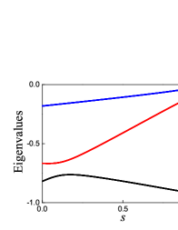
(a)

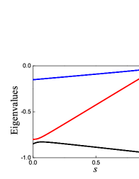
(b)

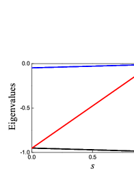
(c)

Figure 4: (Color online) The eigenvalue spectrum of the adiabatic Hamiltonian matrix of an intermediate step by setting $N_{j}/N_{j-1}=1/5$ vs. the parameter $s$ by setting $f=N_{j}/N$ at different values. ($a$) $f=1/15$, ($b$) $f=1/25$, ($c$) $f=1/100$.

The explicit expressions for the eigenvalues of the matrix in Eq. (144) are very complicated. What we are interested is: if the conditions for our algorithm are satisfied, will the conditions for efficiently running the AQC algorithm be satisfied too, i.e., the minimum energy gap between the ground and the first excited states of the adiabatic evolution Hamiltonian be finite? Denote $g=N_{j-1}/N_{j}$ and $f=N_{j}/N$, the matrix in Eq. (144) can be written as

$$\left(\!\!\begin{array}[]{ccc}f(f\!-\!1)\left[s(g-1)\!-g\right]-\!1&f^{2}\left[s(g-1)\!-g\right]\sqrt{g-1\!}&f^{3/2}\sqrt{1\!-\!gf}\left[s(g-1)\!-g\right]\\ f^{2}\left[s(g-1)\!-\!g\right]\sqrt{g\!-\!1\!}&s\left[f^{2}(g\!-\!1)^{2}\!-\!gf\!+\!1\right]\!+\!gf(1\!+\!f\!-\!gf)\!\!-\!\!1&f^{3/2}\!\sqrt{1\!-\!gf}\left[\!s(g\!-\!1)\!-\!g\!\right]\!\sqrt{\!g\!-\!1\!}\\ f^{3/2}\sqrt{1\!-\!gf}\left[s(g-1)\!-g\right]&f^{3/2}\sqrt{1\!-\!gf}\left[s(g-1)\!-g\right]\sqrt{g-1\!}&f(1-gf\!)\left[s(g-1)\!-g\right]\end{array}\!\!\right).$$ (162)

In the main text, we set $N_{j}/N_{j-1}=1/10$, thus the conditions for our algorithm are satisfied. The matrix in Eq. (144) becomes

$$\left(\!\!\begin{array}[]{ccc}f(f\!-\!1)(9s\!-\!10)\!-\!1&3f^{2}(9s\!-\!10)&f^{3/2}\sqrt{1\!-\!10f}(9s\!-\!10)\\ 3f^{2}(9s\!-\!10)&f(81fs\!-\!90f\!-\!10s\!+\!10)\!+\!s\!\!-\!\!1&3f^{3/2}\sqrt{1\!-\!10f}(9s\!-\!10)\\ f^{3/2}\sqrt{1\!-\!10f}(9s\!-\!10)&3f^{3/2}\sqrt{1\!-\!10f}(9s\!-\!10)&f(1\!-\!10f)(9s\!-\!10)\end{array}\!\!\right).$$ (163)

We solve the eigenvalues of the above matrix for $f=1/30,1/50,1/150$, respectively, and draw the energy spectrum vs. $s$ in the main text. We check one more case by setting $N_{j}/N_{j-1}=1/5$, the matrix in Eq. (144) becomes

$$\left(\!\!\begin{array}[]{ccc}f(f\!-\!1)(4s\!-\!5)\!-\!1&2f^{2}(4s\!-\!5)&f^{3/2}\sqrt{1\!-5f}(4s\!-\!5)\\ 2f^{2}(4s\!-\!5)&f(16fs\!-\!20f\!-\!5s\!+\!5)\!+\!s\!\!-\!\!1&2f^{3/2}\sqrt{1\!-\!5f}(4s\!-\!5)\\ f^{3/2}\sqrt{1\!-5f}(4s\!-\!5)&2f^{3/2}\sqrt{1\!-\!5f}(4s\!-\!5)&f(1\!-5f)(4s\!-\!5)\end{array}\!\!\right).$$ (164)

In Fig. $4$, we draw the energy spectrum of the above matrix as a function of $s$ by setting $f=1/15$, $1/25$, and $1/100$, respectively. From the figures we can see that as $f$ becomes small, the minimum energy gap between the ground and the first excited states of the adiabatic evolution Hamiltonians decreases quickly as $s\rightarrow 0$. Comparing with Fig. $2$ in the main text, we can see that as $N_{j}/N_{j-1}$ becomes larger, the minimum energy gap decreases faster as $s\rightarrow 0$. The energy gap between the ground and the first excited states for the case where $N_{j}/N_{j-1}=1/5$ is in the form

$$\Delta E=\frac{1}{2}\left(1+\sqrt{1-20f+200f^{2}-500f^{3}}\right)+5f-1.$$ (165)

We expand the energy gap at $f\rightarrow 0$, that is, the asymptotic limit of $N$, and find that it scales as $O(f^{2})=O(1/N^{2})$. Therefore, the usual quantum adiabatic algorithm cannot be run efficiently by using the same evolution path of our algorithm.

Appendix F Comparison of algorithms for solving the search problem with a special structure

In this paper, we present a quantum algorithm for preparing the ground state of a problem Hamiltonian and apply it for solving a type of search problems with a special structure, and compare with the AQC algorithm (using the same Hamiltonian evolution path as our algorithm and constructing the adiabatic evolution Hamiltonian via linear interpolation of adjacent intermediate Hamiltonians in each step), and the Grover’s algorithm. We now summarize the performance of these algorithms and the phase estimation algorithm (PEA) for solving the structured search problems.

We have shown in the above section that by using the same Hamiltonian evolution path as our algorithm, and constructing the adiabatic evolution Hamiltonian as a linear interpolation between two adjacent intermediate Hamiltonians in each step as $sH_{l-1}+(1-s)H_{l}$, the runtime of the AQC algorithm for solving the structured search problem scales as $O(N^{2})$. In Ref. childs , Childs et al. proposed a method to keep the system in the instantaneous ground state of an adiabatic evolution Hamiltonian by performing Zeno-like measurements. The runtime of this method depends on the minimum energy gap between the ground and the first excited states of the adiabatic evolution Hamiltonian. By using the continuous path of the adiabatic evolution Hamiltonian $sH_{l-1}+(1-s)H_{l}$, the runtime of this method has the same scaling as that of the AQC algorithm with the same adiabatic evolution Hamiltonian. In applying the Grover’s algorithm for solving the structured search problem, the total number of all the $m$ different oracles that are called in the algorithm scales as $O(\sqrt{N})$. The runtime of the algorithm is the same as that of solving the unstructured search problem. The phase estimation algorithm (PEA) is a projective method for obtaining the ground state of a problem Hamiltonian, it projects an initial state onto the ground state of the problem Hamiltonian with probability proportional to the square of the overlap between them. By using the state $|\psi_{0}\rangle=\frac{1}{\sqrt{N}}\sum_{j=0}^{N-1}|j\rangle$, which is an uniform superposition of all the computational basis states, as an initial guess state, the success probability of the PEA for finding the ground state of the structured search problem is $1/N$. Therefore the runtime of the PEA for solving the structured search problem scales as $O(N)$. The runtime of our algorithm for solving the structured search problem is proportional to the number of steps $m$ which scales as $O\left(\log N\right)$, and in each step, the runtime depends on the ratio $N_{j}/N_{j-1}$. The algorithm is efficient as long as $N_{j}/N_{j-1}$ are not exponentially small. In table I, we summarize the performance of the above algorithms for solving the search problem with a special structure.

Algorithms	Runtime	Factors determining the efficiency of the algorithms
AQC	$O\left(N^{2}\right)$	Minimum energy gap between the ground and the first excited states of each adiabatic evolution Hamiltonian.
Grover	$O(\sqrt{N})$	Number of queries of the oracles.
PEA	$O\left(N\right)$	Overlap between a guess state and the ground state of the problem Hamiltonian.
Our algorithm	$O\left(\log N\right)$	Ratio $N_{j}/N_{j-1}$, which are not exponentially small. Here $N_{j}$ represents the number of marked states of $j$-th step.

Table 1: Comparison of the performance of some algorithms for solving the structured search problem. The AQC algorithm and the Grover’s algorithm use the same Hamiltonian evolution path as our algorithm. The term $N$ represents the dimension of the search space. The performance of the method in childs is the same as that of the AQC algorithm.

These algorithms can also be applied for the general case of preparing the ground state of a system. The runtime of the AQC algorithm scales as $O(1/\Delta E_{\min})$, where $\Delta E_{\min}$ is the minimum energy gap between the ground and the first excited states of the adiabatic evolution Hamiltonian. By using the amplitude amplification technique developed from the Grover’s algorithm, quantum algorithm can achieve quadratic speed-up over classical algorithms in preparing the ground state of a system poulin1 . The success probability of the PEA depends on the overlap between an initial guess state and the ground state of the system. Our algorithm requires to construct a Hamiltonian evolution path to reach the system Hamiltonian in order to prepare the ground state of the system, the runtime of the algorithm is proportional to summation of the evolution time of each step, which is proportional to $1/\left(\Delta E\times d\right)$, where $\Delta E$ is the energy gap between the ground and the first excited states of the target intermediate Hamiltonian and $d$ is the overlap between ground states of two adjacent Hamiltonians of the step. The algorithm is efficient if both $\Delta E$ of each Hamiltonian and $d$ of each step are not exponentially small.

References

(1) A. Y. Kitaev, e-print quant-ph/9511026 (1995).
(2) D. S. Abrams and S. Lloyd, Phys. Rev. Lett. 83,
5162 (1999).
(3) D. Poulin and P. Wocjan, Phys. Rev. Lett. 102,
130503 (2009).
(4) E. Farhi, J. Goldstone, S. Gutmann, e-print
quant-ph/0007071v1 (2000).
(5) A. M. Childs, et al., Phys. Rev. A 66,
032314 (2002).
(6) D. Poulin, A. Y. Kitaev, D. S. Steiger, M. B. Hastings, and
M. Troyer, Phys. Rev. Lett. 121, 010501 (2018).
(7) N. J. Cerf, L. K. Grover and C. P. Williams, Phys. Rev. A
61, 032303 (2000).
(8) J. Roland and N. J. Cerf, Phys. Rev. A 68,
062312 (2003).
(9) W. K. Wootters and W. H. Zurek, Nature 299,
802 (1982).
(10) D. Dieks, Phys. Lett. A 92, 271 (1982).
(11) H. Wang, Phys. Rev. A 93, 052334 (2016).
(12) Z. Li, et al., Phys. Rev. Lett. 122, 090504 (2019).
(13) G. H. Low and I. L. Chuang, Phys. Rev. Lett., 118,
010501 (2017).
(14) G. H. Low and I. L. Chuang, Quantum 3,
163 (2019).
(15) T. Monz, et al., Science 351, 1068 (2016).
(16) H. Wang, et al., in preparation.
(17) L. K. Grover, Phys. Rev. Lett. 79, 325-328 (1997).
(18) J. Roland and N. J. Cerf, Phys. Rev. A, 65,
042308 (2002).
(19) T. Albash and D. A. Lidar, Rev. Mod. Phys. 90,
015002 (2018).
(20) D. Aharanov and A. Ta-Shma, e-print arXiv:
quant-ph/0301023v2 (2003); SIAM J. Comput. 37, 47 (2007).
(21) M. B. Hastings, e-print arXiv: 2005.03791v1 (2020)
and references therein.
(22) H. Wang, S. Ashhab and Franco Nori, Physical Review A,
85, 062304 (2012).
(23) C. Cohen-Tannoudji, B. Diu, and F. Laloë, Quantum
Mechanics Vol. 1, p414, (Wiley-Interscience Publication 1977).
(24) P. Shor, Algorithms for quantum computation: discrete
logarithms and factoring. Proc. 35th Ann. Symp. on Found. of Comp. Sci., 124-134 (IEEE Comp. Soc. Press, Los Alamitos, CA, 1994).
(25) E. Farhi, J. Goldstone, S. Gutmann, e-print
quant-ph/arxiv: 1411.4028 (2014).
(26) E. Farhi, J. Goldstone, S. Gutmann, e-print
arxiv:quant-ph/0201031 (2002).