Pairwise Near-maximal Grand Coupling of Brownian Motions

Abstract

The well-known reflection coupling gives a maximal coupling of two one-dimensional Brownian motions with different starting points. Nevertheless, the reflection coupling does not generalize to more than two Brownian motions. In this paper, we construct a coupling of all Brownian motions with all possible starting points (i.e., a grand coupling), such that the coupling for any pair of the coupled processes is close to being maximal, that is, the distribution of the coupling time of the pair approaches that of the maximal coupling as the time tends to $0$ or $\infty$, and the coupling time of the pair is always within a multiplicative factor $2e^{2}$ from the maximal one. We also show that a grand coupling that is pairwise exactly maximal does not exist.

1 Introduction

The maximal coupling of two stochastic processes $P,Q$ is a coupling $(\{X_{t}\}_{t},\{Y_{t}\}_{t})$ (i.e., the marginal distribution of $\{X_{t}\}_{t}$ is $P$, and that of $\{Y_{t}\}_{t}$ is $Q$) that simultaneously maximizes the probability that the processes match after time $s$ (i.e., $X_{t}=Y_{t}$ for all $t\geq s$) for all $s$. It was studied by Griffeath [1], Goldstein [2] and Pitman [3]. For two one-dimensional Brownian motions with different starting points, a maximal coupling can be given by the reflection coupling studied by Lindvall [4], Lindvall and Rogers [5], Hsu and Sturm [6], and Kendall [7]. Also see [8, 9, 10] for results on coupling functionals of Brownian motions.

While the maximal coupling of two stochastic processes exists under rather general conditions [2, 11], it might not exist in the pairwise sense for more than two processes, that is, given a collection of stochastic processes $\{P_{\alpha}\}_{\alpha\in\mathcal{A}}$, there may not exist a coupling $\{\{X_{\alpha,t}\}_{t}\}_{\alpha\in\mathcal{A}}$ (i.e., the marginal distribution of $\{X_{\alpha,t}\}_{t}$ is $P_{\alpha}$) that simultaneously maximizes $\mathbf{P}(\forall t\geq s:\,X_{\alpha,t}=X_{\beta,t})$ for all $s$, $\alpha$, $\beta$. The maximal coalescent coupling, which maximizes the probability that all processes in the collection match after time $s$ (i.e., $\mathbf{P}(\forall\alpha,\beta\in\mathcal{A},\,t\geq s:\,X_{\alpha,t}=X_{\beta,t})$), was studied by Connor [12]. Nevertheless, a maximal coalescent coupling, which only concerns whether the processes all agree after certain time, may not give a maximal (or close to maximal) coupling when only the marginal distribution of a pair of processes $\{X_{\alpha,t}\}_{t}$, $\{X_{\beta,t}\}_{t}$ is considered (refer to Section 2). Other related works on the coupling of more than two distributions or stochastic processes include coupling from the past [13, 14], Wasserstein barycenter [15], and multi-marginal optimal transport [16, 17, 18, 19, 20]. A coupling of Markov chains with the same Markov kernel and all possible initial states (i.e., $P_{\alpha}$ is the Markov chain starting at $\alpha$ for any state $\alpha\in\mathcal{A}$) is often called a grand coupling in the literature on coupling from the past and mixing times of Markov chains (e.g. [21]).

A classical example of a grand coupling of all one-dimensional Brownian motions with all possible starting points (i.e., $P_{\alpha}=\mathrm{BM}(\alpha)$, the Brownian motion starting at $\alpha\in\mathbb{R}$) is the Brownian web studied by Arratia [22] and Tóth and Werner [23]. The Brownian web has a property that, if we consider the marginal joint distribution of the processes with distribution $\mathrm{BM}(\alpha)$ and $\mathrm{BM}(\beta)$ ($\alpha\neq\beta\in\mathbb{R}$), then the processes move independently from $\alpha$ and $\beta$ respectively, until they couple (become equal), and then move together (the same as the Doeblin coupling for Markov chains [24], which is generally not maximal). The distribution of the coupling time between the two processes is the same as the distribution of twice the coupling time of the reflection coupling, i.e., the Brownian web has a multiplicative gap $2$ from the optimum (refer to Section 2). The multiplicative gap does not vanish as the time tends to $0$ or $\infty$.

In this paper, we give a grand coupling $\{\{X_{\alpha,t}\}_{t}\}_{\alpha\in\mathbb{R}}$ of all one-dimensional Brownian motions with all possible starting points (i.e., $\{X_{\alpha,t}\}_{t}$ has marginal $P_{\alpha}=\mathrm{BM}(\alpha)$ for $\alpha\in\mathbb{R}$), called the dyadic grand coupling, such that the coupling for any pair of the coupled processes is close to being maximal. Let

$$\Upsilon_{\alpha,\beta}:=\inf\big{\{}s\geq 0:\,X_{\gamma_{1},t}=X_{\gamma_{2},t},\,\forall\,\gamma_{1},\gamma_{2}\in[\alpha,\beta],t\geq s\big{\}}$$

be the coupling time of all the Brownian motions with starting point lying in the interval $[\alpha,\beta]$, and $\hat{\Upsilon}_{\alpha,\beta}:=\inf\{s\geq 0:\,\hat{X}_{\alpha,t}=\hat{X}_{\beta,t},\,\forall\,t\geq s\}$ be the coupling time of the reflection coupling, where $\{\hat{X}_{\alpha,t}\}_{t\geq 0},\{\hat{X}_{\beta,t}\}_{t\geq 0}$ is the reflection coupling of $\mathrm{BM}(\alpha),\mathrm{BM}(\beta)$ (which is a maximal coupling). Let “$\preceq$” denote first-order stochastic dominance between two real-valued random variables (i.e., $Y\preceq Z$ if $\mathbf{P}(Y\geq t)\leq\mathbf{P}(Z\geq t)$ for all $t\in\mathbb{R}$). Then the distribution of $\Upsilon_{\alpha,\beta}$ is close to that of the optimal $\hat{\Upsilon}_{\alpha,\beta}$ for all $\alpha<\beta$, in the sense that $\Upsilon_{\alpha,\beta}\preceq 2e^{2}\hat{\Upsilon}_{\alpha,\beta}$, and the distribution of $\Upsilon_{\alpha,\beta}$ tends to that of $\hat{\Upsilon}_{\alpha,\beta}$ as the time tends to $0$ or $\infty$ (in the sense of multiplicative gap). More precisely, there exists a function $r:\mathbb{R}_{>0}\to[1,2e^{2}]$ (that does not depend on $\alpha,\beta$) such that $\lim_{t\to 0}r(t)=\lim_{t\to\infty}r(t)=1$, and

$$\hat{\Upsilon}_{\alpha,\beta}\preceq\Upsilon_{\alpha,\beta}\preceq r\left(\frac{\hat{\Upsilon}_{\alpha,\beta}}{|\alpha-\beta|^{2}}\right)\hat{\Upsilon}_{\alpha,\beta}$$ (1.1)

for any $\alpha<\beta$. Numerical evidence shows that the maximum multiplicative gap $2e^{2}$ can be improved to around $1.5$, and the dyadic grand coupling has a strictly smaller coupling time than the Brownian web in the sense of first-order stochastic dominance (see Figure 2.3). Refer to Section 2 for details.

A natural question is whether there exists a grand coupling $\{\{\tilde{X}_{\alpha,t}\}_{t}\}_{\alpha\in\mathbb{R}}$ of $\{\mathrm{BM}(\alpha)\}_{\alpha\in\mathbb{R}}$ such that any pair $\{\tilde{X}_{\alpha,t}\}_{t},\{\tilde{X}_{\beta,t}\}_{t}$ is a maximal coupling. In Section 3, we show that such a pairwise maximal grand coupling does not exist. We conjecture that the dyadic grand coupling is optimal, in the sense of attainable failure probability bounds, as defined in Section 3.

2 Dyadic Grand Coupling of Brownian Motion

Let $\mathrm{BM}(\alpha)$ be the distribution of the standard one-dimensional Brownian motion starting at $\alpha\in\mathbb{R}$ ($P_{\alpha}$ is a probability distribution over the space of continuous functions $\mathrm{C}([0,\infty),\mathbb{R})$ with the topology of uniform convergence over compact subsets of $[0,\infty)$). To couple $\mathrm{BM}(\alpha),\mathrm{BM}(\beta)$ with two different starting points $\alpha,\beta$, the reflection coupling [4, 5] $\{\hat{X}_{\alpha,t}\}_{t\geq 0},\{\hat{X}_{\beta,t}\}_{t\geq 0}$ is given by $\{\hat{X}_{\alpha,t}\}_{t\geq 0}\sim\mathrm{BM}(\alpha)$, $T:=\inf\{t\geq 0:\,\hat{X}_{\alpha,t}=(\alpha+\beta)/2\}$, $\hat{X}_{\beta,t}=\alpha+\beta-\hat{X}_{\alpha,t}$ for $t<T$, $\hat{X}_{\beta,t}=\hat{X}_{\alpha,t}$ for $t\geq T$. The probability of failure of the reflection coupling can be given by

$$\mathbf{P}\Big{(}\exists\,t\geq s\,\mathrm{s.t.}\,\hat{X}_{\alpha,t}\neq\hat{X}_{\beta,t}\Big{)}=\mathrm{erf}\left(\frac{|\alpha-\beta|}{2\sqrt{2s}}\right)$$ (2.1)

for any $s>0$, where

$$\mathrm{erf}(\gamma) :=\int_{-\gamma}^{\gamma}\frac{e^{-x^{2}}}{\sqrt{\pi}}\mathrm{d}x$$

is the error function.

Nevertheless, if we have to couple all the processes in $\{\mathrm{BM}(\alpha)\}_{\alpha\in\mathbb{R}}$, it is impossible to simultaneously attain this probability of failure for all pairs of starting points, as will be shown in Section 3. The maximal coalescent coupling [12] is not useful in this setting since, for any fixed time, it is impossible for all the processes in $\{\{X_{\alpha,t}\}_{t\geq 0}\}_{\alpha\in\mathbb{R}}$ (where $\{X_{\alpha,t}\}_{t\geq 0}\sim\mathrm{BM}(\alpha)$) to coalesce (become all equal) by that time with a positive probability. If we consider only the processes $\{\mathrm{BM}(\alpha)\}_{\alpha\in[\gamma_{1},\gamma_{2}]}$ with starting points in the interval $[\gamma_{1},\gamma_{2}]$, then a maximal coalescent coupling can be given simply by performing the reflection coupling between $\{X_{\gamma_{1},t}\}_{t}$ and $\{X_{\alpha,t}\}_{t}$ for all $\alpha\in(\gamma_{1},\gamma_{2}]$ (note that in the reflection coupling, one process can be obtained deterministically from another, and thus we can express $\{X_{\alpha,t}\}_{t}$ as a function of $\{X_{\gamma_{1},t}\}_{t}\sim\mathrm{BM}(\gamma_{1})$ for all $\alpha\in(\gamma_{1},\gamma_{2}]$). This coupling is undesirable since the coupling time between $\{X_{\gamma_{2},t}\}_{t}$ and $\{X_{\gamma_{2}-\epsilon,t}\}_{t}$ is the same as that between $\{X_{\gamma_{2},t}\}_{t}$ and $\{X_{\gamma_{1},t}\}_{t}$, despite $\mathrm{BM}(\gamma_{2})$ being much closer to $\mathrm{BM}(\gamma_{2}-\epsilon)$ than to $\mathrm{BM}(\gamma_{1})$.

The Brownian web [22, 23] $\{\{X_{\alpha,t}^{\mathrm{BW}}\}_{t\geq 0}\}_{\alpha\in\mathbb{R}}$ (where $\{X_{\alpha,t}^{\mathrm{BW}}\}_{t\geq 0}\sim\mathrm{BM}(\alpha)$) gives a probability of failure

$$\mathbf{P}\Big{(}\exists\,t\geq s\,\mathrm{s.t.}\,X_{\alpha,t}^{\mathrm{BW}}\neq X_{\beta,t}^{\mathrm{BW}}\Big{)}$$

$$=\mathbf{P}\Big{(}\exists\,\gamma_{1},\gamma_{2}\in[\alpha,\beta],t\geq s\,\mathrm{s.t.}\,X_{\gamma_{1},t}^{\mathrm{BW}}\neq X_{\gamma_{2},t}^{\mathrm{BW}}\Big{)}$$

$$=\mathrm{erf}\left(\frac{|\alpha-\beta|}{2\sqrt{s}}\right),$$

and hence the distribution of the coupling time between $\{X_{\alpha,t}^{\mathrm{BW}}\}_{t}$ and $\{X_{\beta,t}^{\mathrm{BW}}\}_{t}$ (the first time where $X_{\alpha,t}^{\mathrm{BW}}=X_{\beta,t}^{\mathrm{BW}}$) is the same as the distribution of twice the coupling time of the reflection coupling $\{\hat{X}_{\alpha,t}\}_{t},\{\hat{X}_{\beta,t}\}_{t}$. The multiplicative gap $2$ does not vanish as the time tends to $0$ or $\infty$, that is, the Brownian web does not satisfy (1.1).

In this section, we propose a coupling that achieves a probability of failure close to that of the reflection coupling for all pairs of starting points. We construct a coupling $\{\{X_{\alpha,t}\}_{t\geq 0}\}_{\alpha\in\mathbb{R}}$ (where $\{X_{\alpha,t}\}_{t\geq 0}\sim\mathrm{BM}(\alpha)$) as follows.

Definition 1 (Dyadic grand coupling of Brownian motion).

Let $\{Y_{t}\}_{t\geq 0}\sim\mathrm{BES}^{3}(0)$, the Bessel process of dimension $3$ starting at $0$. Let $W_{i}\stackrel{{\scriptstyle iid}}{{\sim}}\mathrm{Unif}\{\pm 1\}$ for $i\in\mathbb{Z}$ be independent of $\{Y_{t}\}_{t\geq 0}$. For any $\theta\in[0,1]$ and $\alpha\in\mathbb{R}$, let

$$G_{\theta,\alpha,j}=G_{\theta,\alpha,j}(\{W_{i}\}_{i\leq j}):=\begin{cases}W_{j}&\mathrm{if}\;\left(\alpha-\sum_{k=-\infty}^{j-1}W_{k}2^{k+\theta-1}\!+2^{j+\theta-1}\right)\mathrm{mod}\;2^{j+\theta+1}\in[0,2^{j+\theta}),\\ -W_{j}&\mathrm{otherwise},\end{cases}$$

for $j\in\mathbb{Z}$, where $a\;\mathrm{mod}\;b:=a-b\lfloor a/b\rfloor$ for $b>0$. By the definition of $G_{\theta,\alpha,j}$, the conditional distribution of $G_{\theta,\alpha,j}$ given any $\{W_{k}\}_{k<j}$ is $\mathrm{Unif}\{\pm 1\}$ (since $W_{j}\sim\mathrm{Unif}\{\pm 1\}$ independent of $\{W_{k}\}_{k<j}$). Hence $G_{\theta,\alpha,j}\stackrel{{\scriptstyle iid}}{{\sim}}\mathrm{Unif}\{\pm 1\}$, and is independent of $\{Y_{t}\}_{t\geq 0}$.

As will be shown in Appendix A, if $\sup\{j:W_{j}=1\}=\sup\{j:W_{j}=-1\}=\infty$ (which happens almost surely), then

$$\left\lfloor 2^{-(j+\theta)}\left(\alpha-\!\sum_{k=-\infty}^{j-1}W_{k}2^{k+\theta-1}\right)+\frac{1}{2}\right\rfloor=\sum_{k=j}^{\infty}(W_{k}-G_{\theta,\alpha,k})2^{k-j-1}$$ (2.2)

for any $j\in\mathbb{Z}$,

$$\sum_{j=-\infty}^{\infty}(W_{j}-G_{\theta,\alpha,j})2^{j+\theta-1}=\alpha,$$ (2.3)

and $G_{\theta,\alpha,j}=W_{j}$ for all sufficiently large $j$. For $\theta\in[0,1]$ and $i\in\mathbb{Z}$, let

$$T_{\theta,i}:=\inf\left\{t\geq 0:\,Y_{t}=2^{i+\theta}\right\}.$$

Let $X_{\theta,\alpha,0}:=\alpha$. For $t>0$, with $i$ defined to satisfy $T_{\theta,i-1}<t\leq T_{\theta,i}$, let

$$X_{\theta,\alpha,t} :=\alpha+\sum_{j=-\infty}^{i-1}G_{\theta,\alpha,j}2^{j+\theta-1}+(Y_{t}-2^{i+\theta-1})G_{\theta,\alpha,i}$$ (2.4)

$$=(Y_{t}-2^{i+\theta})G_{\theta,\alpha,i}+\sum_{j=-\infty}^{\infty}(W_{j}-\mathbf{1}\{j>i\}G_{\theta,\alpha,j})2^{j+\theta-1},$$ (2.5)

where the equivalence of (2.4) and (2.5) can be seen by (2.3). Let $\Theta\sim\mathrm{Unif}[0,1]$ be independent of $(\{Y_{t}\}_{t\geq 0},\{W_{i}\}_{i})$, and let $X_{\alpha,t}:=X_{\Theta,\alpha,t}$.

We now check that $\{X_{\alpha,t}\}_{t\geq 0}\sim\mathrm{BM}(\alpha)$. First, for any $i$, we can see from (2.4) that $\lim_{t\searrow T_{\theta,i-1}}X_{\theta,\alpha,t}=X_{\theta,\alpha,T_{\theta,i-1}}$, and hence $\{X_{\alpha,t}\}_{t\geq 0}$ is continuous in $t$.

By the strong Markov property, $\{Y_{t+T_{\theta,i-1}}\}_{t\geq 0}\sim\mathrm{BES}^{3}(2^{i+\theta-1})$. Since $\mathrm{BES}^{3}(2^{i+\theta-1})$ is the distribution of $\mathrm{BM}(2^{i+\theta-1})$ conditioned to stay positive [25, 26, 27, 28], we see that $\{Y_{t+T_{\theta,i-1}}\}_{0\leq t\leq T_{\theta,i}-T_{\theta,i-1}}$ has the same distribution as $\mathrm{BM}(2^{i+\theta-1})$ conditioned to stay positive and stopped when it hits $2^{i+\theta}$, or equivalently, stopped when it hits either $0$ or $2^{i+\theta}$ and conditioned on the event that it hits $2^{i+\theta}$ (which has probability $1/2$, so the conditioning is well-defined). By symmetry, $\{(Y_{t+T_{\theta,i-1}}-2^{i+\theta-1})G_{\theta,\alpha,i}\}_{0\leq t\leq T_{\theta,i}-T_{\theta,i-1}}$ has the same distribution as $\mathrm{BM}(0)$ stopped when it hits either $2^{i+\theta-1}$ or $-2^{i+\theta-1}$, and is independent of $(T_{\theta,i-1},\{Y_{t}\}_{t\leq T_{\theta,i-1}},\{G_{\theta,\alpha,j}\}_{j\leq i-1})$ (since $G_{\theta,\alpha,j}\stackrel{{\scriptstyle iid}}{{\sim}}\mathrm{Unif}\{\pm 1\}$ independent of $\{Y_{t}\}_{t\geq 0}$). Welding these processes together, we can see from (2.4) that $\{X_{\theta,\alpha,t+T_{\theta,i}}-X_{\theta,\alpha,T_{\theta,i}}\}_{t\geq 0}$ follows $\mathrm{BM}(0)$ and is independent of $(T_{\theta,i},\{Y_{t}\}_{t\leq T_{\theta,i}},\{G_{\theta,\alpha,j}\}_{j\leq i})$ for any $\theta,\alpha,i$. Since a random process with continuous sample paths is characterized by its finite-dimensional marginals, by letting $i\to-\infty$, we see that $\{X_{\theta,\alpha,t}\}_{t\geq 0}\sim\mathrm{BM}(\alpha)$ for any $\theta,\alpha$. Hence $\{X_{\alpha,t}\}_{t\geq 0}\sim\mathrm{BM}(\alpha)$.

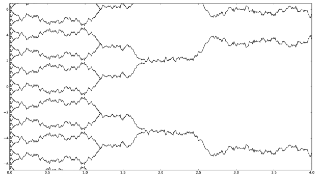
Figure 2.1: A sample of the dyadic grand coupling, where all the processes $\{\{X_{\alpha,t}\}_{t}\}_{\alpha\in\mathbb{R}}$ are plotted together. Note that the coalescence points (the points where two processes join) at the same time are evenly spaced on the space axis. The processes after the time of each coalescence point can be regarded as performing the reflection coupling between adjacent pairs of coalescence points.

We then evaluate the probability of failure of this coupling.

Theorem 2.

For the dyadic grand coupling of Brownian motion $\{\{X_{\alpha,t}\}_{t\geq 0}\}_{\alpha\in\mathbb{R}}$, we have

$$\mathbf{P}\Big{(}\exists\,t\geq s\,\mathrm{s.t.}\,X_{\alpha,t}\neq X_{\beta,t}\Big{)}$$

$$=\mathbf{P}\Big{(}\exists\,\gamma_{1},\gamma_{2}\in[\alpha,\beta],t\geq s\,\mathrm{s.t.}\,X_{\gamma_{1},t}\neq X_{\gamma_{2},t}\Big{)}$$

$$=\int_{\psi/2}^{\infty}\left(\sum_{k=1}^{\infty}2(-1)^{k+1}\exp\left(-\frac{k^{2}\pi^{2}}{2\zeta^{2}}\right)\right)\frac{\zeta^{-2}\psi}{\ln 2}\left(\min\left\{\zeta\psi^{-1},\,1\right\}-\frac{1}{2}\right)\mathrm{d}\zeta$$

for any $\alpha<\beta$ and $s>0$, where $\psi:=|\alpha-\beta|/\sqrt{s}$.

As a consequence, we have the following results.

Corollary 3.

Let $\{\{X_{\alpha,t}\}_{t\geq 0}\}_{\alpha\in\mathbb{R}}$ be the one-dimensional dyadic grand coupling of Brownian motion. Fix any $\alpha<\beta$. Let $\{\hat{X}_{\alpha,t}\}_{t\geq 0},\{\hat{X}_{\beta,t}\}_{t\geq 0}$ be the reflection coupling of $\mathrm{BM}(\alpha),\mathrm{BM}(\beta)$. Let $\Upsilon_{\alpha,\beta}:=\inf\{s\geq 0:\,X_{\gamma_{1},t}=X_{\gamma_{2},t},\,\forall\,\gamma_{1},\gamma_{2}\in[\alpha,\beta],t\geq s\}$ and $\hat{\Upsilon}_{\alpha,\beta}:=\inf\{s\geq 0:\,\hat{X}_{\alpha,t}=\hat{X}_{\beta,t},\,\forall\,t\geq s\}$ be the coupling times of the dyadic grand coupling and the reflection coupling respectively. Let $F_{\Upsilon_{\alpha,\beta}}^{-1}(p):=\inf\{s:\,\mathbf{P}(\Upsilon_{\alpha,\beta}\leq s)\geq p\}$ be the inverse distribution function of $\Upsilon_{\alpha,\beta}$, and define $F_{\hat{\Upsilon}_{\alpha,\beta}}^{-1}(p)$ similarly. We have:

1. For any $s>0$ (let $\psi:=|\alpha-\beta|/\sqrt{s}$),

   $$\mathbf{P}(\Upsilon_{\alpha,\beta}>s)\leq\frac{\psi}{\sqrt{2\pi}}.$$

   As a result,

   $$\lim_{s\to\infty}\frac{\mathbf{P}(\Upsilon_{\alpha,\beta}>s)}{\mathbf{P}(\hat{\Upsilon}_{\alpha,\beta}>s)}=1,$$

   and

   $$\lim_{p\to 1}\frac{F_{\Upsilon_{\alpha,\beta}}^{-1}(p)}{F_{\hat{\Upsilon}_{\alpha,\beta}}^{-1}(p)}=1,$$

   i.e., the tail of the distribution of the coupling time of the dyadic grand coupling approaches that of the reflection coupling as $s\to\infty$.

2. For any $s>0$ (let $\psi:=|\alpha-\beta|/\sqrt{s}$), if $\psi\geq 2\sqrt{2}$, then

   $$\mathbf{P}(\Upsilon_{\alpha,\beta}>s)\leq 1-\left(1-\left(\mathrm{erf}\left(\frac{\psi+8/\psi}{2\sqrt{2}}\right)\right)^{3}\right)\frac{\ln(1+8/\psi^{2})+(1+8/\psi^{2})^{-1}-1}{\ln 2}.$$

   As a result,

   $$\lim_{p\to 0}\frac{F_{\Upsilon_{\alpha,\beta}}^{-1}(p)}{F_{\hat{\Upsilon}_{\alpha,\beta}}^{-1}(p)}=1,$$

   i.e., the multiplicative gap between $\Upsilon_{\alpha,\beta}$ and $\hat{\Upsilon}_{\alpha,\beta}$ vanishes as $s\to 0$.

3. For any $s>0$ (let $\psi:=|\alpha-\beta|/\sqrt{s}$),

   $$\mathbf{P}(\Upsilon_{\alpha,\beta}>s)\leq\mathrm{erf}\left(\frac{e\psi}{2}\right).$$

   As a result, $2e^{2}\hat{\Upsilon}_{\alpha,\beta}$ first-order stochastically dominates $\Upsilon_{\alpha,\beta}$, i.e., the dyadic grand coupling is pairwise within a multiplicative factor $2e^{2}$ from being maximal.

These three bounds imply (1.1) by taking

$$r(t):=\frac{1}{t}F_{\Upsilon_{0,1}}^{-1}(F_{\hat{\Upsilon}_{0,1}}(t)).$$

Note that $\Upsilon_{\alpha,\beta}/|\alpha-\beta|^{2}$ has the same distribution as $\Upsilon_{0,1}$, and $\hat{\Upsilon}_{\alpha,\beta}/|\alpha-\beta|^{2}$ has the same distribution as $\hat{\Upsilon}_{0,1}$.

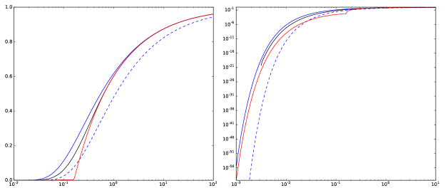
Figure 2.2: Plot of the cumulative distribution function $F_{\Upsilon_{0,1}}$ (black), $F_{\hat{\Upsilon}_{0,1}}$ (blue), the bound on $F_{\Upsilon_{0,1}}$ in Corollary 3 (red) (we take the pointwise maximum of the three bounds in Corollary 3), and the cumulative distribution function of the coupling time of the Brownian web (dashed line). The left figure is in log-scale for the x-axis, whereas the right figre is in log-scale for both axes. Note that $F_{\Upsilon_{0,1}}$ (the black curve) is bounded between the blue curve and the red curve. Due to numerical precision issue, $F_{\Upsilon_{0,1}}(t)$ is not plotted for small $t$’s in the right figure.

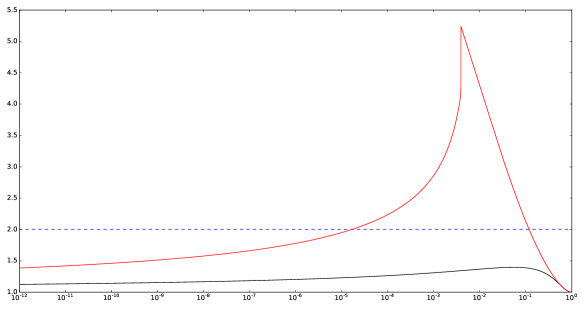
Figure 2.3: Plot of $F_{\Upsilon_{\alpha,\beta}}^{-1}(p)/F_{\hat{\Upsilon}_{\alpha,\beta}}^{-1}(p)$ (black), the upper bound on $F_{\Upsilon_{\alpha,\beta}}^{-1}(p)/F_{\hat{\Upsilon}_{\alpha,\beta}}^{-1}(p)$ in Corollary 3 (red), and the corresponding ratio for the Brownian web (dashed line, which is constantly $2$) against $p$, where $\alpha<\beta$ (these curves do not depend on the choice of $\alpha,\beta$). While Corollary 3 gives a multiplicative gap $2e^{2}$, we can observe in this graph that the multiplicative gap can be improved to around $1.5$, since $F_{\Upsilon_{\alpha,\beta}}^{-1}(p)/F_{\hat{\Upsilon}_{\alpha,\beta}}^{-1}(p)$ stays below $1.5$ for all $p$.

We first prove Theorem 2.

Proof of Theorem 2.

Let $I$ be such that $T_{\Theta,I-1}<s\leq T_{\Theta,I}$. We have

$$\mathbf{P}\Big{(}\exists\,t\geq s\;\mathrm{s.t.}\,X_{\alpha,t}\neq X_{\beta,t}\Big{)}$$

$$\stackrel{{\scriptstyle(a)}}{{=}}\mathbf{P}\left(\exists\,k\geq I\;\mathrm{s.t.}\,G_{\Theta,\alpha,k}\neq G_{\Theta,\beta,k}\right)$$

$$=\mathbf{P}\left(\exists\,k\geq I\;\mathrm{s.t.}\,\sum_{j=k}^{\infty}(W_{j}-G_{\Theta,\alpha,j})2^{j-k-1}\neq\sum_{j=k}^{\infty}(W_{j}-G_{\Theta,\beta,j})2^{j-k-1}\right)$$

$$\stackrel{{\scriptstyle(b)}}{{=}}\mathbf{P}\left(\exists\,k\geq I\;\mathrm{s.t.}\,\left\lfloor 2^{-(k+\Theta)}\!\left(\!\alpha\!-\!\sum_{j=-\infty}^{k-1}W_{j}2^{j+\Theta-1}\!\right)\!+\frac{1}{2}\right\rfloor\neq\left\lfloor 2^{-(k+\Theta)}\!\left(\!\beta\!-\!\sum_{j=-\infty}^{k-1}W_{j}2^{j+\Theta-1}\!\right)\!+\frac{1}{2}\right\rfloor\right)$$

$$=\mathbf{P}\left(s\leq T_{\Theta,\max\left\{k:\,\left\lfloor 2^{-(k+\Theta)}\left(\alpha-\sum_{j=-\infty}^{k-1}W_{j}2^{j+\Theta-1}\right)+\frac{1}{2}\right\rfloor\neq\left\lfloor 2^{-(k+\Theta)}\left(\beta-\sum_{j=-\infty}^{k-1}W_{j}2^{j+\Theta-1}\right)+\frac{1}{2}\right\rfloor\right\}}\right)$$

$$=\mathbf{P}\left(\sup_{t\leq s}Y_{t}\leq 2^{\max\left\{k:\,\left\lfloor 2^{-(k+\Theta)}\left(\alpha-\sum_{j=-\infty}^{k-1}W_{j}2^{j+\Theta-1}\right)+\frac{1}{2}\right\rfloor\neq\left\lfloor 2^{-(k+\Theta)}\left(\beta-\sum_{j=-\infty}^{k-1}W_{j}2^{j+\Theta-1}\right)+\frac{1}{2}\right\rfloor\right\}+\Theta}\right)$$ (2.6)

$$\stackrel{{\scriptstyle(c)}}{{=}}\mathbf{E}\left[\sum_{k=1}^{\infty}2(-1)^{k+1}\exp\left(-\frac{k^{2}\pi^{2}}{2Z^{2}}\right)\right],$$

where

$$Z:=s^{-1/2}2^{\max\left\{k:\,\left\lfloor 2^{-(k+\Theta)}\left(\alpha-\sum_{j=-\infty}^{k-1}W_{j}2^{j+\Theta-1}\right)+\frac{1}{2}\right\rfloor\neq\left\lfloor 2^{-(k+\Theta)}\left(\beta-\sum_{j=-\infty}^{k-1}W_{j}2^{j+\Theta-1}\right)+\frac{1}{2}\right\rfloor\right\}+\Theta}.$$

Here (a) comes from (2.5), (b) is due to (2.2), and (c) is because $(\pi/2)\sqrt{s}/\sup_{t\leq s}Y_{t}$ follows the Kolmogorov distribution [29, 30]. By the same arguments,

$$\mathbf{P}\Big{(}\exists\,\gamma_{1},\gamma_{2}\in[\alpha,\beta],t\geq s\;\mathrm{s.t.}\,X_{\gamma_{1},t}\neq X_{\gamma_{2},t}\Big{)}$$

$$=\mathbf{P}\left(\exists\,\gamma_{1},\gamma_{2}\in[\alpha,\beta],k\geq I\;\mathrm{s.t.}\,G_{\Theta,\gamma_{1},k}\neq G_{\Theta,\gamma_{2},k}\right)$$

$$=\!\mathbf{P}\!\!\left(\!\exists\,\gamma_{1},\!\gamma_{2}\!\in\![\alpha,\beta],k\!\geq\!I\,\mathrm{s.t.}\left\lfloor 2^{-(k+\Theta)}\!\!\left(\!\gamma_{1}\!-\!\!\!\!\sum_{j=-\infty}^{k-1}\!\!\!W_{j}2^{j+\Theta-1}\!\right)\!\!+\!\frac{1}{2}\right\rfloor\!\neq\!\left\lfloor 2^{-(k+\Theta)}\!\!\left(\!\gamma_{2}\!-\!\!\!\!\sum_{j=-\infty}^{k-1}\!\!\!W_{j}2^{j+\Theta-1}\!\right)\!\!+\!\frac{1}{2}\right\rfloor\!\right)$$

$$=\mathbf{P}\left(\exists\,k\geq I\;\mathrm{s.t.}\,\left\lfloor 2^{-(k+\Theta)}\!\left(\!\alpha\!-\!\sum_{j=-\infty}^{k-1}W_{j}2^{j+\Theta-1}\!\right)\!+\frac{1}{2}\right\rfloor\neq\left\lfloor 2^{-(k+\Theta)}\!\left(\!\beta\!-\!\sum_{j=-\infty}^{k-1}W_{j}2^{j+\Theta-1}\!\right)\!+\frac{1}{2}\right\rfloor\right),$$

and hence the two probabilities in Theorem 2 are equal.

To find the distribution of $Z$, we have

$$\mathbf{P}\left(\max\left\{k:\,\left\lfloor 2^{-(k+\theta)}\left(\alpha-\sum_{j=-\infty}^{k-1}W_{j}2^{j+\theta-1}\right)+\frac{1}{2}\right\rfloor\neq\left\lfloor 2^{-(k+\theta)}\left(\beta-\sum_{j=-\infty}^{k-1}W_{j}2^{j+\theta-1}\right)+\frac{1}{2}\right\rfloor\right\}\geq l\right)$$

$$\stackrel{{\scriptstyle(a)}}{{=}}\mathbf{P}\left(\exists\,k\geq l\,\mathrm{s.t.}\,\sum_{j=k}^{\infty}(W_{j}-G_{\theta,\alpha,j})2^{j-k-1}\neq\sum_{j=k}^{\infty}(W_{j}-G_{\theta,\beta,j})2^{j-k-1}\right)$$

$$=\mathbf{P}\left(\sum_{j=l}^{\infty}(W_{j}-G_{\theta,\alpha,j})2^{j-l-1}\neq\sum_{j=l}^{\infty}(W_{j}-G_{\theta,\beta,j})2^{j-l-1}\right)$$

$$\stackrel{{\scriptstyle(b)}}{{=}}\mathbf{P}\left(\left\lfloor 2^{-(l+\theta)}\left(\alpha-\sum_{j=-\infty}^{l-1}W_{j}2^{j+\theta-1}\right)+\frac{1}{2}\right\rfloor\neq\left\lfloor 2^{-(l+\theta)}\left(\beta-\sum_{j=-\infty}^{l-1}W_{j}2^{j+\theta-1}\right)+\frac{1}{2}\right\rfloor\right)$$

$$\stackrel{{\scriptstyle(c)}}{{=}}\frac{1}{2}\int_{-1}^{1}\mathbf{1}\left\{\left\lfloor 2^{-(l+\theta)}\left(\alpha-\gamma 2^{l+\theta-1}\right)+\frac{1}{2}\right\rfloor\neq\left\lfloor 2^{-(l+\theta)}\left(\beta-\gamma 2^{l+\theta-1}\right)+\frac{1}{2}\right\rfloor\right\}\mathrm{d}\gamma$$

$$=\min\left\{2^{-(l+\theta)}|\alpha-\beta|,\,1\right\},$$

where (a) and (b) are due to (2.2), and (c) is because $\sum_{j=-\infty}^{l-1}W_{j}2^{j+\theta-1}\sim\mathrm{Unif}[-2^{l+\theta-1},2^{l+\theta-1}]$. Therefore,

$$\mathbf{P}\left(Z\geq\zeta\right)$$

$$=\mathbf{P}\Bigg{(}\max\left\{k:\,\left\lfloor 2^{-(k+\Theta)}\left(\alpha-\sum_{j=-\infty}^{k-1}W_{j}2^{j+\Theta-1}\right)+\frac{1}{2}\right\rfloor\neq\left\lfloor 2^{-(k+\Theta)}\left(\beta-\sum_{j=-\infty}^{k-1}W_{j}2^{j+\Theta-1}\right)+\frac{1}{2}\right\rfloor\right\}$$

$$\;\;\;\;\;\;\geq\left\lceil\log_{2}(\zeta\sqrt{s})-\Theta\right\rceil\Bigg{)}$$

$$=\int_{0}^{1}\min\left\{2^{-(\lceil\log_{2}(\zeta\sqrt{s})-\theta\rceil+\theta)}|\alpha-\beta|,\,1\right\}\mathrm{d}\theta$$

$$=\int_{0}^{1}\min\left\{2^{-(\log_{2}(\zeta\sqrt{s})+\theta)}|\alpha-\beta|,\,1\right\}\mathrm{d}\theta$$

$$=\int_{0}^{1}\min\left\{\zeta^{-1}s^{-1/2}2^{-\theta}|\alpha-\beta|,\,1\right\}\mathrm{d}\theta$$

$$=\int_{0}^{1}\min\left\{\zeta^{-1}2^{-\theta}\psi,\,1\right\}\mathrm{d}\theta,$$

where $\psi:=|\alpha-\beta|/\sqrt{s}$. Hence,

$$-\frac{\mathrm{d}}{\mathrm{d}\zeta}\mathbf{P}\left(Z\geq\zeta\right)$$

$$=-\int_{0}^{1}\frac{\mathrm{d}}{\mathrm{d}\zeta}\min\left\{\zeta^{-1}2^{-\theta}\psi,\,1\right\}\mathrm{d}\theta$$

$$=\int_{0}^{1}\mathbf{1}\left\{\zeta^{-1}2^{-\theta}\psi\leq 1\right\}\zeta^{-2}2^{-\theta}\psi\mathrm{d}\theta$$

$$=\zeta^{-2}\psi\int_{\min\{\max\{\log_{2}(\zeta^{-1}\psi),\,0\},\,1\}}^{1}2^{-\theta}\mathrm{d}\theta$$

$$=\frac{\zeta^{-2}\psi}{\ln 2}\left(2^{-\min\{\max\{\log_{2}(\zeta^{-1}\psi),\,0\},\,1\}}-\frac{1}{2}\right),$$

and thus

$$\mathbf{P}\Big{(}\exists\,\gamma_{1},\gamma_{2}\in[\alpha,\beta],t\geq s\,\mathrm{s.t.}\,X_{\gamma_{1},t}\neq X_{\gamma_{2},t}\Big{)}$$

$$=\int_{0}^{\infty}\left(\sum_{k=1}^{\infty}2(-1)^{k+1}\exp\left(-\frac{k^{2}\pi^{2}}{2\zeta^{2}}\right)\right)\frac{\zeta^{-2}\psi}{\ln 2}\left(2^{-\min\{\max\{\log_{2}(\zeta^{-1}\psi),\,0\},\,1\}}-\frac{1}{2}\right)\mathrm{d}\zeta$$

$$=\int_{\psi/2}^{\infty}\left(\sum_{k=1}^{\infty}2(-1)^{k+1}\exp\left(-\frac{k^{2}\pi^{2}}{2\zeta^{2}}\right)\right)\frac{\zeta^{-2}\psi}{\ln 2}\left(\min\left\{\zeta\psi^{-1},\,1\right\}-\frac{1}{2}\right)\mathrm{d}\zeta.$$

∎

We then prove Corollary 3.

Proof of Corollary 3.

We first prove Corollary 3.1. By Theorem 2,

$$\mathbf{P}\Big{(}\exists\,\gamma_{1},\gamma_{2}\in[\alpha,\beta],t\geq s\,\mathrm{s.t.}\,X_{\gamma_{1},t}\neq X_{\gamma_{2},t}\Big{)}$$

$$=\int_{\psi/2}^{\infty}\left(\sum_{k=1}^{\infty}2(-1)^{k+1}\exp\left(-\frac{k^{2}\pi^{2}}{2\zeta^{2}}\right)\right)\frac{\zeta^{-2}\psi}{\ln 2}\left(\min\left\{\zeta\psi^{-1},\,1\right\}-\frac{1}{2}\right)\mathrm{d}\zeta$$

$$=\sum_{k=1}^{\infty}2(-1)^{k+1}\int_{\psi/2}^{\infty}\exp\left(-\frac{k^{2}\pi^{2}}{2\zeta^{2}}\right)\frac{\zeta^{-2}\psi}{\ln 2}\left(\min\left\{\zeta\psi^{-1},\,1\right\}-\frac{1}{2}\right)\mathrm{d}\zeta$$

$$=\sum_{k=1}^{\infty}2(-1)^{k+1}\left(\frac{\frac{\psi}{\sqrt{2\pi}k}\mathrm{erf}\left(\frac{\pi k}{\sqrt{2}\psi}\right)-\mathrm{Ei}\left(-\frac{\pi^{2}k^{2}}{2\psi^{2}}\right)}{2\ln 2}-\frac{\frac{\psi}{\sqrt{2\pi}k}\mathrm{erf}\left(\frac{\sqrt{2}\pi k}{\psi}\right)-\mathrm{Ei}\left(-\frac{2\pi^{2}k^{2}}{\psi^{2}}\right)}{2\ln 2}+\frac{\frac{\psi}{\sqrt{2\pi}k}\mathrm{erf}\left(\frac{\pi k}{\sqrt{2}\psi}\right)}{2\ln 2}\right)$$

$$=\frac{1}{\ln 2}\sum_{k=1}^{\infty}(-1)^{k+1}\left(\frac{2\psi}{\sqrt{2\pi}k}\mathrm{erf}\left(\frac{\pi k}{\sqrt{2}\psi}\right)-\frac{\psi}{\sqrt{2\pi}k}\mathrm{erf}\left(\frac{\sqrt{2}\pi k}{\psi}\right)-\mathrm{Ei}\left(-\frac{\pi^{2}k^{2}}{2\psi^{2}}\right)+\mathrm{Ei}\left(-\frac{2\pi^{2}k^{2}}{\psi^{2}}\right)\right),$$

where $\mathrm{Ei}(\gamma):=-\int_{-\gamma}^{\infty}(e^{-x}/x)\mathrm{d}x$ is the exponential integral function. We have

$$\left.\frac{\mathrm{d}}{\mathrm{d}\psi}\mathbf{P}\Big{(}\exists\,\gamma_{1},\gamma_{2}\in[\alpha,\beta],t\geq s\,\mathrm{s.t.}\,X_{\gamma_{1},t}\neq X_{\gamma_{2},t}\Big{)}\right|_{\psi=0}$$

$$=\frac{1}{\ln 2}\sum_{k=1}^{\infty}(-1)^{k+1}\left.\frac{\mathrm{d}}{\mathrm{d}\psi}\left(\frac{2\psi}{\sqrt{2\pi}k}\mathrm{erf}\left(\frac{\pi k}{\sqrt{2}\psi}\right)-\frac{\psi}{\sqrt{2\pi}k}\mathrm{erf}\left(\frac{\sqrt{2}\pi k}{\psi}\right)-\mathrm{Ei}\left(-\frac{\pi^{2}k^{2}}{2\psi^{2}}\right)+\mathrm{Ei}\left(-\frac{2\pi^{2}k^{2}}{\psi^{2}}\right)\right)\right|_{\psi=0}$$

$$=\frac{1}{\ln 2}\sum_{k=1}^{\infty}(-1)^{k+1}\left(\frac{2}{\sqrt{2\pi}k}-\frac{1}{\sqrt{2\pi}k}\right)$$

$$=\frac{1}{\sqrt{2\pi}\ln 2}\sum_{k=1}^{\infty}\frac{(-1)^{k+1}}{k}$$

$$=\frac{1}{\sqrt{2\pi}}.$$ (2.7)

Also, for any $\alpha_{1}<\alpha_{2}<\alpha_{3}$,

$$\mathbf{P}\Big{(}\exists\,\gamma_{1},\gamma_{2}\in[\alpha_{1},\alpha_{3}],t\geq s\,\mathrm{s.t.}\,X_{\gamma_{1},t}\neq X_{\gamma_{2},t}\Big{)}$$

$$\leq\mathbf{P}\Big{(}\exists\,\gamma_{1},\gamma_{2}\in[\alpha_{1},\alpha_{2}],t\geq s\,\mathrm{s.t.}\,X_{\gamma_{1},t}\neq X_{\gamma_{2},t}\Big{)}+\mathbf{P}\Big{(}\exists\,\gamma_{1},\gamma_{2}\in[\alpha_{2},\alpha_{3}],t\geq s\,\mathrm{s.t.}\,X_{\gamma_{1},t}\neq X_{\gamma_{2},t}\Big{)}.$$

Hence $\mathbf{P}(\exists\,\gamma_{1},\gamma_{2}\in[\alpha,\beta],t\geq s\,\mathrm{s.t.}\,X_{\gamma_{1},t}\neq X_{\gamma_{2},t})$ (which only depends on $\psi$) is subadditive in $\psi$ (in fact, it is shown in Appendix B that it is concave). Combining this with (2.7), we have

$$\mathbf{P}\Big{(}\exists\,\gamma_{1},\gamma_{2}\in[\alpha,\beta],t\geq s\,\mathrm{s.t.}\,X_{\gamma_{1},t}\neq X_{\gamma_{2},t}\Big{)}\leq\frac{\psi}{\sqrt{2\pi}}.$$

For Corollary 3.3, if $\psi\geq 2$, by (2.6),

$$\mathbf{P}\Big{(}\exists\,\gamma_{1},\gamma_{2}\in[\alpha,\beta],t\geq s\,\mathrm{s.t.}\,X_{\gamma_{1},t}\neq X_{\gamma_{2},t}\Big{)}$$

$$=\mathbf{P}\big{(}\sup_{t\leq s}Y_{t}\leq\sqrt{s}Z\big{)}$$

$$=\mathbf{P}\big{(}\sup_{t\leq 1}Y_{t}\leq Z\big{)}$$

$$\stackrel{{\scriptstyle(a)}}{{\leq}}\mathbf{P}\big{(}\sup_{t\leq 1}B_{1,t}\leq Z\;\mathrm{and}\;\sup_{t\leq 1}B_{2,t}\leq Z\;\mathrm{and}\;\sup_{t\leq 1}B_{3,t}\leq Z\big{)}$$

$$=\mathbf{E}\left[\left(\mathrm{erf}\left(Z/\sqrt{2}\right)\right)^{3}\right]$$

$$\leq\mathbf{E}\left[\mathrm{erf}\left(\exp(\ln Z)/\sqrt{2}\right)\right]$$

$$\stackrel{{\scriptstyle(b)}}{{\leq}}\mathrm{erf}\left(\exp(\mathbf{E}\left[\ln Z\right])/\sqrt{2}\right),$$

where in (a), we let $Y_{t}=\sqrt{B_{1,t}^{2}+B_{2,t}^{2}+B_{3,t}^{2}}$, where $\{B_{1,t}\}_{t},\{B_{2,t}\}_{t},\{B_{3,t}\}_{t}$ are independent Brownian motions, and (b) is because $\gamma\mapsto\mathrm{erf}(\exp(\gamma)/\sqrt{2})$ is concave for $\gamma\geq 0$ (note that $Z\geq\psi/2\geq 1$). We have

$$\mathbf{E}\left[\ln Z\right]$$

$$=\int_{\psi/2}^{\infty}(\ln\zeta)\frac{\zeta^{-2}\psi}{\ln 2}\left(\min\left\{\zeta\psi^{-1},\,1\right\}-\frac{1}{2}\right)\mathrm{d}\zeta$$

$$=\frac{\psi\ln\psi+\psi+\psi(\ln\psi)^{2}}{2\psi\ln 2}-\frac{\psi\ln(\psi/2)+\psi+(\psi/2)(\ln(\psi/2))^{2}}{2(\psi/2)\ln 2}+\frac{\psi}{2\ln 2}\cdot\frac{\ln\psi+1}{\psi}$$

$$=\frac{\ln\psi+1+(\ln\psi)^{2}}{2\ln 2}-\frac{2\ln\psi-2\ln 2+2+(\ln\psi-\ln 2)^{2}}{2\ln 2}+\frac{\ln\psi+1}{2\ln 2}$$

$$=\frac{1}{2\ln 2}\left((\ln\psi)^{2}-(\ln\psi-\ln 2)^{2}\right)+1$$

$$=\frac{1}{2\ln 2}(2\ln\psi-\ln 2)\ln 2+1$$

$$=\ln\psi-\frac{\ln 2}{2}+1.$$

Therefore,

$$\mathbf{P}\Big{(}\exists\,\gamma_{1},\gamma_{2}\in[\alpha,\beta],t\geq s\,\mathrm{s.t.}\,X_{\gamma_{1},t}\neq X_{\gamma_{2},t}\Big{)}$$

$$\leq\mathrm{erf}\left(\frac{1}{\sqrt{2}}\exp\left(\ln\psi-\frac{\ln 2}{2}+1\right)\right)$$

$$=\mathrm{erf}\left(\frac{e\psi}{2}\right).$$

If $\psi<2$, then

$$\mathbf{P}\Big{(}\exists\,\gamma_{1},\gamma_{2}\in[\alpha,\beta],t\geq s\,\mathrm{s.t.}\,X_{\gamma_{1},t}\neq X_{\gamma_{2},t}\Big{)}$$

$$\leq\frac{\psi}{\sqrt{2\pi}}$$

$$\leq\mathrm{erf}\left(\frac{e\psi}{2}\right).$$

The result follows.

For Corollary 3.2, for any $1<\delta\leq 2$,

$$\mathbf{P}\Big{(}\exists\,\gamma_{1},\gamma_{2}\in[\alpha,\beta],t\geq s\,\mathrm{s.t.}\,X_{\gamma_{1},t}\neq X_{\gamma_{2},t}\Big{)}$$

$$\leq\mathbf{E}\left[\left(\mathrm{erf}\left(Z/\sqrt{2}\right)\right)^{3}\right]$$

$$\leq 1-\left(1-\left(\mathrm{erf}\left(\frac{\psi\delta}{2\sqrt{2}}\right)\right)^{3}\right)\mathbf{P}(Z\leq\psi\delta/2)$$

$$=1-\left(1-\left(\mathrm{erf}\left(\frac{\psi\delta}{2\sqrt{2}}\right)\right)^{3}\right)\int_{\psi/2}^{\psi\delta/2}\frac{\zeta^{-2}\psi}{\ln 2}\left(\min\left\{\zeta\psi^{-1},\,1\right\}-\frac{1}{2}\right)\mathrm{d}\zeta$$

$$=1-\left(1-\left(\mathrm{erf}\left(\frac{\psi\delta}{2\sqrt{2}}\right)\right)^{3}\right)\left(\frac{\psi}{2(\ln 2)(\psi\delta/2)}+\frac{\ln(\psi\delta/2)}{\ln 2}-\frac{\psi}{2(\ln 2)(\psi/2)}-\frac{\ln(\psi/2)}{\ln 2}\right)$$

$$=1-\left(1-\left(\mathrm{erf}\left(\frac{\psi\delta}{2\sqrt{2}}\right)\right)^{3}\right)\frac{\ln\delta+\delta^{-1}-1}{\ln 2}$$

If $\psi\geq 2\sqrt{2}$, substituting $\delta=1+8/\psi^{2}$, we have

$$\mathbf{P}\Big{(}\exists\,\gamma_{1},\gamma_{2}\in[\alpha,\beta],t\geq s\,\mathrm{s.t.}\,X_{\gamma_{1},t}\neq X_{\gamma_{2},t}\Big{)}$$

$$\leq 1-\left(1-\left(\mathrm{erf}\left(\frac{\psi+8/\psi}{2\sqrt{2}}\right)\right)^{3}\right)\frac{\ln(1+8/\psi^{2})+(1+8/\psi^{2})^{-1}-1}{\ln 2}$$

$$\leq 1-\left(1-\mathrm{erf}\left(\frac{\psi+8/\psi}{2\sqrt{2}}\right)\right)\frac{\ln(1+8/\psi^{2})+(1+8/\psi^{2})^{-1}-1}{\ln 2}.$$

Note that $\ln(1+8/\psi^{2})+(1+8/\psi^{2})^{-1}-1=\Omega(\psi^{-4})$ as $\psi\to\infty$, whereas $1-\mathrm{erf}(x)\to 0$ exponentially as $x\to\infty$. Therefore there exists a function $\kappa:\mathbb{R}_{>0}\to\mathbb{R}_{>0}$ such that $\lim_{t\to\infty}\kappa(t)=0$, and

$$\mathbf{P}\Big{(}\exists\,\gamma_{1},\gamma_{2}\in[\alpha,\beta],t\geq s\,\mathrm{s.t.}\,X_{\gamma_{1},t}\neq X_{\gamma_{2},t}\Big{)}$$

$$\leq\mathrm{erf}\left(\frac{(1+\kappa(t))\psi}{2\sqrt{2}}\right).$$

This implies that

$$\lim_{p\to 0}\frac{F_{\Upsilon_{\alpha,\beta}}^{-1}(p)}{F_{\hat{\Upsilon}_{\alpha,\beta}}^{-1}(p)}=1.$$

∎

3 Nonexistence of a Pairwise Maximal Coupling

In this section, we show that there does not exist a pairwise maximal coupling $\{\{\tilde{X}_{\alpha,t}\}_{t\geq 0}\}_{\alpha\in\mathbb{R}}$ of $\{\mathrm{BM}(\alpha)\}_{\alpha\in\mathbb{R}}$, that is, one in which every pair $\{\tilde{X}_{\alpha,t}\}_{t\geq 0},\{\tilde{X}_{\beta,t}\}_{t\geq 0}$ is a maximal coupling, i.e.,

$$\mathbf{P}\Big{(}\exists\,t\geq s\,\mathrm{s.t.}\,\tilde{X}_{\alpha,t}\neq\tilde{X}_{\beta,t}\Big{)}=\mathrm{erf}\left(\frac{|\alpha-\beta|}{2\sqrt{2s}}\right).$$ (3.1)

Note that both (3.1) and the expression in Theorem 2 depend only on $\psi:=|\alpha-\beta|/\sqrt{s}$.

Definition 4.

We say that a function $h:[0,\infty)\to[0,1]$ is an attainable failure probability bound if there exists a coupling $\{\{\tilde{X}_{\alpha,t}\}_{t\geq 0}\}_{\alpha\in\mathbb{R}}$ of $\{\mathrm{BM}(\alpha)\}_{\alpha\in\mathbb{R}}$ such that

$$\mathbf{P}\left(\exists\,t\geq s\,\mathrm{s.t.}\,\tilde{X}_{\alpha,t}\neq\tilde{X}_{\beta,t}\right)\leq h\left(\frac{|\alpha-\beta|}{\sqrt{s}}\right)$$

for all $\alpha,\beta,\in\mathbb{R}$, $s>0$. We say that $c>0$ is an attainable multiplicative gap if $x\mapsto\mathrm{erf}(x\sqrt{c}/(2\sqrt{2}))$ is an attainable failure probability bound.

One attainable failure probability bound is given in Theorem 2. Corollary 3.3 implies that $2e^{2}$ is an attainable multiplicative gap. A pairwise maximal coupling exists if and only if $x\mapsto\mathrm{erf}(x/(2\sqrt{2}))$ is an attainable failure probability bound, or equivalently, $1$ is an attainable multiplicative gap.

We now prove a lower bound on any attainable failure probability bound which implies a lower bound on the attainable multiplicative gap. This implies the nonexistence of a pairwise maximal coupling.

Theorem 5.

If $h$ is a failure probability bound, then for any $0<s<t$, we have

$$\tilde{h}\left(\frac{2}{\sqrt{t}}\right)+\tilde{h}\left(\frac{2}{\sqrt{s}}\right)+2\tilde{h}\left(\frac{1}{\sqrt{s}}\right)$$

$$\geq\mathrm{erfc}\left(\frac{1}{\sqrt{2t}}\right)-\mathrm{erfc}\left(\frac{1}{\sqrt{2s}}\right)-\mathrm{erfc}\left(\frac{1}{4\sqrt{2(t-s)}}\right),$$

where $\tilde{h}(x):=h(x)-\mathrm{erf}(x/(2\sqrt{2}))$, and $\mathrm{erfc}(x):=1-\mathrm{erf}(x)$. Hence $x\mapsto\mathrm{erf}(x/(2\sqrt{2}))$ is not an attainable failure probability bound. Moreover, $1.0025$ is not an attainable multiplicative gap.

Proof.

For any $\alpha<\beta$, $s>0$, we have

$$\mathbf{P}\left(X_{\beta,s}\leq(\alpha+\beta)/2\;\mathrm{and}\;X_{\beta,s}\neq X_{\alpha,s}\right)+\mathbf{P}\left(X_{\alpha,s}\geq(\alpha+\beta)/2\;\mathrm{and}\;X_{\beta,s}\neq X_{\alpha,s}\right)$$

$$=\mathbf{P}(X_{\beta,s}\leq(\alpha+\beta)/2)+\mathbf{P}(X_{\alpha,s}\geq(\alpha+\beta)/2)$$

$$\;\;\;-\left(\mathbf{P}\left(X_{\beta,s}\leq(\alpha+\beta)/2\;\mathrm{and}\;X_{\beta,s}=X_{\alpha,s}\right)+\mathbf{P}\left(X_{\alpha,s}\geq(\alpha+\beta)/2\;\mathrm{and}\;X_{\beta,s}=X_{\alpha,s}\right)\right)$$

$$\leq\mathbf{P}(X_{\beta,s}\leq(\alpha+\beta)/2)+\mathbf{P}(X_{\alpha,s}\geq(\alpha+\beta)/2)-\mathbf{P}(X_{\beta,s}=X_{\alpha,s})$$

$$\stackrel{{\scriptstyle(a)}}{{\leq}}1-\mathrm{erf}\left(\frac{|\alpha-\beta|}{2\sqrt{2s}}\right)-\left(1-h\left(\frac{|\alpha-\beta|}{\sqrt{s}}\right)\right)$$

$$=\tilde{h}\left(\frac{|\alpha-\beta|}{\sqrt{s}}\right),$$ (3.2)

where (a) is because $X_{\alpha,s}\sim\mathrm{N}(\alpha,s)$, $X_{\beta,s}\sim\mathrm{N}(\beta,s)$ and by the definition of the failure probability bound.

Let $0<s<t$. We have

$$\mathbf{P}\left(X_{1,s}-X_{-1,s}\leq 1/2\;\mathrm{and}\;X_{1,s}\neq X_{-1,s}\right)$$

$$\leq\mathbf{P}\left(X_{1,s}\leq 0\;\mathrm{and}\;X_{1,s}\neq X_{-1,s}\right)+\mathbf{P}\left(X_{-1,s}\geq 0\;\mathrm{and}\;X_{1,s}\neq X_{-1,s}\right)$$

$$\;\;\;+\mathbf{P}\left(X_{1,s}\leq 1/2\;\mathrm{and}\;X_{-1,s}\geq 1/2\;\mathrm{and}\;X_{1,s}\neq X_{-1,s}\right)$$

$$\stackrel{{\scriptstyle(a)}}{{\leq}}\mathbf{P}\left(X_{1,s}\leq 0\;\mathrm{and}\;X_{1,s}\neq X_{-1,s}\right)+\mathbf{P}\left(X_{-1,s}\geq 0\;\mathrm{and}\;X_{1,s}\neq X_{-1,s}\right)$$

$$\;\;\;+\mathbf{P}\left(X_{1,s}\leq 1/2\;\mathrm{and}\;X_{1,s}\neq X_{0,s}\right)+\mathbf{P}\left(X_{-1,s}\geq 1/2\;\mathrm{and}\;X_{-1,s}\neq X_{0,s}\right)$$

$$\stackrel{{\scriptstyle(b)}}{{\leq}}\tilde{h}(2/\sqrt{s})+2\tilde{h}(1/\sqrt{s}),$$

where (a) is because if $X_{1,s}\neq X_{-1,s}$, then either $X_{1,s}\neq X_{0,s}$ or $X_{-1,s}\neq X_{0,s}$, and (b) is by applying (3.2) on $(\alpha,\beta,s)\leftarrow(-1,1,s)$, $(0,1,s)$ and $(-1,0,s)$ respectively. Hence,

$$\mathbf{P}\left(X_{1,t}=X_{-1,t}\;\mathrm{and}\;X_{1,s}\neq X_{-1,s}\right)$$

$$\leq\mathbf{P}\left(X_{1,s}-X_{-1,s}\leq 1/2\;\mathrm{and}\;X_{1,s}\neq X_{-1,s}\right)$$

$$\;\;+\mathbf{P}(X_{1,t}-X_{1,s}\leq-1/4)+\mathbf{P}(X_{-1,t}-X_{-1,s}\geq 1/4)$$

$$\leq\tilde{h}(2/\sqrt{s})+2\tilde{h}(1/\sqrt{s})+\mathrm{erfc}\left(\frac{1/4}{\sqrt{2(t-s)}}\right).$$

Therefore,

$$1-h(2/\sqrt{t})$$

$$\leq\mathbf{P}(X_{1,t}=X_{-1,t})$$

$$\leq\mathbf{P}(X_{1,s}=X_{-1,s})+\mathbf{P}\left(X_{1,t}=X_{-1,t}\;\mathrm{and}\;X_{1,s}\neq X_{-1,s}\right)$$

$$\leq\mathrm{erfc}\left(\frac{2}{2\sqrt{2s}}\right)+\tilde{h}(2/\sqrt{s})+2\tilde{h}(1/\sqrt{s})+\mathrm{erfc}\left(\frac{1/4}{\sqrt{2(t-s)}}\right)$$

$$=\mathrm{erfc}\left(\frac{1}{\sqrt{2s}}\right)+\mathrm{erfc}\left(\frac{1}{4\sqrt{2(t-s)}}\right)+\tilde{h}(2/\sqrt{s})+2\tilde{h}(1/\sqrt{s}).$$

Hence,

$$\tilde{h}\left(\frac{2}{\sqrt{t}}\right)+\tilde{h}\left(\frac{2}{\sqrt{s}}\right)+2\tilde{h}\left(\frac{1}{\sqrt{s}}\right)$$

$$\geq\mathrm{erfc}\left(\frac{1}{\sqrt{2t}}\right)-\mathrm{erfc}\left(\frac{1}{\sqrt{2s}}\right)-\mathrm{erfc}\left(\frac{1}{4\sqrt{2(t-s)}}\right).$$

Note that the above lower bound can be positive (e.g. it is at least $0.0019$ when $s=0.33$, $t=0.3348$), and thus $x\mapsto\mathrm{erf}(x/(2\sqrt{2}))$ is not an attainable failure probability bound.

It can be verified numerically that $x\mapsto\mathrm{erf}(x\sqrt{c}/(2\sqrt{2}))$ does not satisfy the above inequality when $c=1.0025$, $s=0.2361$, $t=0.2408$. Hence $1.0025$ is not an attainable multiplicative gap. ∎

We conjecture that the dyadic grand coupling is optimal in the following sense.

Conjecture 6.

If $h$ is a failure probability bound, then for any $\psi>0$, we have

$$h(\psi)\geq\int_{\psi/2}^{\infty}\left(\sum_{k=1}^{\infty}2(-1)^{k+1}\exp\left(-\frac{k^{2}\pi^{2}}{2\zeta^{2}}\right)\right)\frac{\zeta^{-2}\psi}{\ln 2}\left(\min\left\{\zeta\psi^{-1},\,1\right\}-\frac{1}{2}\right)\mathrm{d}\zeta,$$

i.e., the attainable failure probability bound given in Theorem 2 is pointwise optimal.

Loosely speaking, the dyadic grand coupling is “locally a reflection coupling”, in the sense that the coupled processes after the time of each coalescence point can be obtained by performing the reflection coupling between adjacent pairs of coalescence points (see Figure 2.1). In Conjecture 6, we raise the question whether such “locally optimal” coupling is globally optimal.

It may also be of interest to find the smallest attainable multiplicative gap. Theorem 5 and the numerical evidence in Figure 2.3 show that the infimum of the set of attainable multiplicative gaps is between $1.0025$ and $1.5$.

4 Conclusions and Discussion

We constructed a coupling of $\{\mathrm{BM}(\alpha)\}_{\alpha\in\mathbb{R}}$, such that the coupling for any pair of the coupled processes is close to being maximal. While it is shown that a pairwise exactly maximal coupling does not exist, we conjecture that our coupling is optimal among couplings of $\{\mathrm{BM}(\alpha)\}_{\alpha\in\mathbb{R}}$ in the sense of attainable failure probability bounds.

One future direction is to generalize the construction to Brownian motions in $\mathbb{R}^{n}$. While we can couple each coordinate independently using the dyadic grand coupling, this may not be the optimal construction.

Another direction is to consider Brownian motions with initial distributions (rather than fixed starting points), i.e., the collection of processes is $\{\mathrm{BM}(P)\}_{P\in\mathcal{P}(\mathbb{R})}$, where $\mathcal{P}(\mathbb{R})$ is the set of distributions over $\mathbb{R}$, and $\mathrm{BM}(P)$ is the Brownian motion with initial distribution $P$. One simple construction is to first couple the starting point by the quantile coupling, then apply the dyadic grand coupling, i.e., $X_{P,0}:=F_{P}^{-1}(U)$, where $U\sim\mathrm{Unif}[0,1]$, and $X_{P,t}:=X_{X_{P,0},t}$ for $t>0$, where $X_{X_{P,0},t}$ is given by the dyadic grand coupling with starting point $X_{P,0}$. Another construction is to use the sequential Poisson functional representation [20] instead of the quantile coupling, since it is more suitable for minimizing concave costs (it is shown in Appendix B that the probability of failure in Theorem 2 is concave in $|\alpha-\beta|$).

5 Acknowledgements

The authors acknowledge support from the NSF grants CNS-1527846, CCF-1618145, CCF-1901004, the NSF Science & Technology Center grant CCF-0939370 (Science of Information), and the William and Flora Hewlett Foundation supported Center for Long Term Cybersecurity at Berkeley.

Appendix A Proof of the Claim in Definition 1

We first prove that for any $\theta\in[0,1]$, $\alpha\in\mathbb{R}$, we have $G_{\theta,\alpha,j}=W_{j}$ for all sufficiently large $j$, as long as $\sup\{j:W_{j}=1\}=\sup\{j:W_{j}=-1\}=\infty$. Let $k_{1}\in\mathbb{Z}$ be such that $2^{k_{1}}>4|\alpha|$ and $W_{k_{1}}=1$, and $k_{-1}\in\mathbb{Z}$ be such that $2^{k_{-1}}>4|\alpha|$ and $W_{k_{-1}}=-1$. Assume $j\geq\max\{k_{1},k_{-1}\}$. We have

$$\alpha-\sum_{k=-\infty}^{j-1}W_{k}2^{k+\theta-1}$$

$$\leq\alpha+\sum_{k\leq j-1,\,k\neq k_{1}}2^{k+\theta-1}-2^{k_{1}+\theta-1}$$

$$=\alpha+2^{j+\theta-1}-2^{k_{1}+\theta}$$

$$<2^{j+\theta-1},$$

where the last inequality is by the definition of $k_{1}$. Similarly, $\alpha-\sum_{k=-\infty}^{j-1}W_{k}2^{k+\theta-1}>-2^{j+\theta-1}$. Hence,

$$\left(\alpha-\sum_{k=-\infty}^{j-1}W_{k}2^{k+\theta-1}\!+2^{j+\theta-1}\right)\mathrm{mod}\;2^{j+\theta+1}\in[0,2^{j+\theta}),$$

and $G_{\theta,\alpha,j}=W_{j}$.

We then prove (2.2). We will prove by induction that for all $j\in\mathbb{Z}$,

$$\left\lfloor 2^{-(j+\theta)}\left(\alpha-\sum_{k=-\infty}^{j-1}W_{k}2^{k+\theta-1}\!+2^{j+\theta-1}\right)\right\rfloor$$

$$=2^{-(j+\theta)}\sum_{k=j}^{\infty}(W_{k}-G_{\theta,\alpha,k})2^{k+\theta-1}.$$

If $j\geq\max\{k_{1},k_{-1}\}$, then $-2^{j+\theta-1}<\alpha-\sum_{k=-\infty}^{j-1}W_{k}2^{k+\theta-1}<2^{j+\theta-1}$, and also $W_{k}=G_{\theta,\alpha,k}$ for $k\geq j$, and thus both sides in the induction hypothesis are $0$.

Assume the induction hypothesis is true for $j+1$. If $W_{j}=G_{\theta,\alpha,j}$, then

$$\left(\alpha-\sum_{k=-\infty}^{j-1}W_{k}2^{k+\theta-1}\!+2^{j+\theta-1}\right)\mathrm{mod}\;2^{j+\theta+1}\in[0,2^{j+\theta}),$$

and hence

$$\left\lfloor 2^{-(j+\theta)}\left(\alpha-\sum_{k=-\infty}^{j-1}W_{k}2^{k+\theta-1}\!+2^{j+\theta-1}\right)\right\rfloor$$

$$\stackrel{{\scriptstyle(a)}}{{=}}2\left\lfloor 2^{-(j+\theta+1)}\left(\alpha-\sum_{k=-\infty}^{j-1}W_{k}2^{k+\theta-1}\!+2^{j+\theta-1}+(1-W_{j})2^{j+\theta-1}\right)\right\rfloor$$

$$=2\left\lfloor 2^{-(j+\theta+1)}\left(\alpha-\sum_{k=-\infty}^{j}W_{k}2^{k+\theta-1}\!+2^{j+\theta}\right)\right\rfloor$$

$$\stackrel{{\scriptstyle(b)}}{{=}}2\cdot 2^{-(j+1+\theta)}\sum_{k=j+1}^{\infty}(W_{k}-G_{\theta,\alpha,k})2^{k+\theta-1}$$

$$=2^{-(j+\theta)}\sum_{k=j}^{\infty}(W_{k}-G_{\theta,\alpha,k})2^{k+\theta-1},$$

where (a) is because $(1-W_{j})2^{j+\theta-1}\in[0,2^{j+\theta}]$, and (b) is by the induction hypothesis for $j+1$. Therefore the induction hypothesis holds for $j$. If $W_{j}=-G_{\theta,\alpha,j}$, then

$$\left(\alpha-\sum_{k=-\infty}^{j-1}W_{k}2^{k+\theta-1}\!+2^{j+\theta-1}\right)\mathrm{mod}\;2^{j+\theta+1}\in[2^{j+\theta},2^{j+\theta+1}),$$

and hence

$$\left\lfloor 2^{-(j+\theta)}\left(\alpha-\sum_{k=-\infty}^{j-1}W_{k}2^{k+\theta-1}\!+2^{j+\theta-1}\right)\right\rfloor$$

$$\stackrel{{\scriptstyle(a)}}{{=}}2\left\lfloor 2^{-(j+\theta+1)}\left(\alpha-\sum_{k=-\infty}^{j-1}W_{k}2^{k+\theta-1}\!+2^{j+\theta-1}+(1-W_{j})2^{j+\theta-1}\right)\right\rfloor+W_{j}$$

$$=2\left\lfloor 2^{-(j+\theta+1)}\left(\alpha-\sum_{k=-\infty}^{j}W_{k}2^{k+\theta-1}\!+2^{j+\theta}\right)\right\rfloor+W_{j}$$

$$=2\cdot 2^{-(j+1+\theta)}\sum_{k=j+1}^{\infty}(W_{k}-G_{\theta,\alpha,k})2^{k+\theta-1}+W_{j}$$

$$=2^{-(j+\theta)}\sum_{k=j}^{\infty}(W_{k}-G_{\theta,\alpha,k})2^{k+\theta-1},$$

where (a) can be deduced by considering whether $W_{j}=1$ or $-1$. Therefore the induction hypothesis holds for $j$.

Hence the induction hypothesis holds for all $j\in\mathbb{Z}$, and

$$\sum_{k=j}^{\infty}(W_{k}-G_{\theta,\alpha,k})2^{k+\theta-1}\!-2^{j+\theta-1}\leq\alpha-\!\sum_{k=-\infty}^{j-1}W_{k}2^{k+\theta-1}\!<\sum_{k=j}^{\infty}(W_{k}-G_{\theta,\alpha,k})2^{k+\theta-1}\!+2^{j+\theta-1}.$$

Letting $j\to-\infty$, we have $\sum_{j=-\infty}^{\infty}(W_{j}-G_{\theta,\alpha,j})2^{j+\theta-1}=\alpha$.

Appendix B Proof that the Expression in Theorem 2 is concave in $|\alpha-\beta|$

Let $h(\psi):=\mathbf{P}(\exists\,\gamma_{1},\gamma_{2}\in[0,\psi],t\geq 1\,\mathrm{s.t.}\,X_{\gamma_{1},t}\neq X_{\gamma_{2},t})$ be given in Theorem 2. Let $0<\psi_{1}<\psi_{2}$. Fix $l>\psi_{2}$. Let $(A_{1},B_{1}),(A_{2},B_{2}),\ldots,(A_{N},B_{N})\subseteq[0,l]$ be maximal open intervals with length at least $\psi_{1}$, sorted in ascending order, such that $\{X_{\gamma,t}\}_{t\geq 1}$ is constant within each interval (i.e., for any $i=1,\ldots,N$, we have $B_{i}-A_{i}\geq\psi_{1}$, $\{X_{\gamma_{1},t}\}_{t\geq 1}=\{X_{\gamma_{2},t}\}_{t\geq 1}$ for any $\gamma_{1},\gamma_{2}\in(A_{i},B_{i})$, and any open interval in $[0,l]$ that is a proper superset of $(A_{i},B_{i})$ does not have this property). For any $\rho\in[0,1]$, let $\psi:=\rho\psi_{1}+(1-\rho)\psi_{2}$. We have

$$h(\psi) =\frac{1}{l-\psi}\int_{0}^{l-\psi}\mathbf{P}(\exists\,\gamma_{1},\gamma_{2}\in[x,x+\psi],t\geq 1\,\mathrm{s.t.}\,X_{\gamma_{1},t}\neq X_{\gamma_{2},t})\mathrm{d}x$$

$$=1-\frac{1}{l-\psi}\mathbf{E}\left[\sum_{i=1}^{N}\max\{B_{i}-A_{i}-\psi,0\}\right]$$

$$\stackrel{{\scriptstyle(a)}}{{\geq}}1-\frac{1}{l-\psi}\mathbf{E}\left[\sum_{i=1}^{N}\left(\rho\max\{B_{i}-A_{i}-\psi_{1},0\}+(1-\rho)\max\{B_{i}-A_{i}-\psi_{2},0\}\right)\right]$$

$$=1-\frac{1}{l-\psi}\left(\rho\mathbf{E}\left[\sum_{i=1}^{N}\max\{B_{i}-A_{i}-\psi_{1},0\}\right]+(1-\rho)\mathbf{E}\left[\sum_{i=1}^{N}\max\{B_{i}-A_{i}-\psi_{2},0\}\right]\right)$$

$$=1-\frac{1}{l-\psi}\left(\rho(l-\psi_{1})(1-h(\psi_{1}))+(1-\rho)(l-\psi_{2})(1-h(\psi_{2}))\right),$$

where (a) is by the convexity of $x\mapsto\max\{\gamma-x,0\}$. Letting $l\to\infty$, we have $h(\psi)\geq\rho h(\psi_{1})+(1-\rho)h(\psi_{2})$. Hence $h$ is concave on $(0,\infty)$. Since $h$ is non-decreasing, $h$ is concave on $[0,\infty)$.

References

[1]
D. Griffeath, “A maximal coupling for Markov chains,” Probability
Theory and Related Fields, vol. 31, no. 2, pp. 95–106, 1975.
[2]
S. Goldstein, “Maximal coupling,” Probability Theory and Related
Fields, vol. 46, no. 2, pp. 193–204, 1979.
[3]
J. Pitman, “On coupling of Markov chains,” Probability Theory and
Related Fields, vol. 35, no. 4, pp. 315–322, 1976.
[4]
T. Lindvall, “On coupling of Brownian motions,” Technical Report
1982:23, Dept. Mathematics, Chalmers Univ. Technology and Univ.
Göteborg, 1982.
[5]
T. Lindvall and L. C. G. Rogers, “Coupling of multidimensional diffusions by
reflection,” The Annals of Probability, vol. 14, no. 3, pp. 860–872,
1986.
[6]
E. P. Hsu and K.-T. Sturm, “Maximal coupling of Euclidean Brownian
motions,” Communications in Mathematics and Statistics, vol. 1,
no. 1, pp. 93–104, 2013.
[7]
W. S. Kendall, “Coupling, local times, immersions,” Bernoulli,
vol. 21, no. 2, pp. 1014–1046, 2015.
[8]
G. B. Arous, M. Cranston, and W. S. Kendall, “Coupling constructions for
hypoelliptic diffusions: Two examples,” in Proc. Symp. Pure Math,
vol. 57, 1995, p. 193.
[9]
W. Kendall and C. Price, “Coupling iterated Kolmogorov diffusions,”
Electronic Journal of Probability, vol. 9, pp. 382–410, 2004.
[10]
W. S. Kendall, “Coupling all the Lévy stochastic areas of
multidimensional Brownian motion,” The Annals of Probability,
vol. 35, no. 3, pp. 935–953, 2007.
[11]
H. Thorisson, “On maximal and distributional coupling,” The Annals of
Probability, pp. 873–876, 1986.
[12]
S. Connor, “Coupling: Cutoffs, CFTP and tameness,” Ph.D. dissertation,
University of Warwick, 2007.
[13]
J. G. Propp and D. B. Wilson, “Exact sampling with coupled Markov chains and
applications to statistical mechanics,” Random Structures &
Algorithms, vol. 9, no. 1-2, pp. 223–252, 1996.
[14]
J. Propp and D. Wilson, “Coupling from the past: a user’s guide,”
Microsurveys in Discrete Probability, vol. 41, pp. 181–192, 1998.
[15]
M. Agueh and G. Carlier, “Barycenters in the Wasserstein space,” SIAM
Journal on Mathematical Analysis, vol. 43, no. 2, pp. 904–924, 2011.
[16]
H. G. Kellerer, “Duality theorems for marginal problems,” Zeitschrift
für Wahrscheinlichkeitstheorie und verwandte Gebiete, vol. 67, no. 4,
pp. 399–432, 1984.
[17]
W. Gangbo and A. Święch, “Optimal maps for the multidimensional
Monge-Kantorovich problem,” Communications on Pure and Applied
Mathematics: A Journal Issued by the Courant Institute of Mathematical
Sciences, vol. 51, no. 1, pp. 23–45, 1998.
[18]
B. Pass, “Uniqueness and Monge solutions in the multimarginal optimal
transportation problem,” SIAM Journal on Mathematical Analysis,
vol. 43, no. 6, pp. 2758–2775, 2011.
[19]
O. Angel and Y. Spinka, “Pairwise optimal coupling of multiple random
variables,” arXiv preprint arXiv:1903.00632, 2019.
[20]
C. T. Li and V. Anantharam, “Pairwise multi-marginal optimal transport and
embedding for earth mover’s distance,” arXiv preprint
arXiv:1908.01388, 2019.
[21]
D. A. Levin, M. J. Luczak, and Y. Peres, “Glauber dynamics for the mean-field
Ising model: cut-off, critical power law, and metastability,”
Probability Theory and Related Fields, vol. 146, no. 1-2, p. 223,
2010.
[22]
R. A. Arratia, “Coalescing Brownian motions on the line,” Ph.D.
dissertation, University of Wisconsin–Madison, 1979.
[23]
B. Tóth and W. Werner, “The true self-repelling motion,”
Probability Theory and Related Fields, vol. 111, no. 3, pp. 375–452,
1998.
[24]
W. Doeblin, “Exposé de la théorie des chaınes simples constantes de
Markov á un nombre fini d’états,” Mathématique de
l’Union Interbalkanique, vol. 2, no. 77-105, pp. 78–80, 1938.
[25]
H. P. McKean, “Excursions of a non-singular diffusion,” Probability
Theory and Related Fields, vol. 1, no. 3, pp. 230–239, 1963.
[26]
F. B. Knight, “Brownian local times and taboo processes,” Transactions
of the American Mathematical Society, vol. 143, pp. 173–185, 1969.
[27]
D. Williams, “Path decomposition and continuity of local time for
one-dimensional diffusions, I,” Proceedings of the London
Mathematical Society, vol. 3, no. 4, pp. 738–768, 1974.
[28]
J. W. Pitman, “One-dimensional Brownian motion and the three-dimensional
Bessel process,” Advances in Applied Probability, vol. 7, no. 3,
pp. 511–526, 1975.
[29]
A. N. Borodin and P. Salminen, Handbook of Brownian motion-facts and
formulae. Birkhäuser, 2012.
[30]
J. Pitman and M. Yor, “The law of the maximum of a Bessel bridge,”
Electron. J. Probab, vol. 4, no. 15, pp. 1–35, 1999.