Natural Actor-Critic Converges Globally for
Hierarchical Linear Quadratic Regulator

Abstract

Multi-agent reinforcement learning has been successfully applied to a number of challenging problems. Despite these empirical successes, theoretical understanding of different algorithms is lacking, primarily due to the curse of dimensionality caused by the exponential growth of the state-action space with the number of agents. We study a fundamental problem of multi-agent linear quadratic regulator (LQR) in a setting where the agents are partially exchangeable. In this setting, we develop a hierarchical actor-critic algorithm, whose computational complexity is independent of the total number of agents, and prove its global linear convergence to the optimal policy. As LQRs are often used to approximate general dynamic systems, this paper provides an important step towards a better understanding of general hierarchical mean-field multi-agent reinforcement learning.

Keywords: Markov Decision Process, Linear Quadratic Regulator, Actor-Critic Algorithms, Multi-Agent Reinforcement Learning, Mean-Field Reinforcement Learning

1 Introduction

Multi-agent reinforcement learning (MARL) (Bu et al., 2008) combined with deep neural networks has recently been applied successfully to problems ranging from self-driving cars (Shalev-Shwartz et al., 2016) and robotics (Yang and Gu, 2004) to E-sports (Vinyals et al., 2019; OpenAI, 2018) and Go (Silver et al., 2016, 2017). Despite promising empirical results in few specific domains, MARL remains challenging both in theory and practice as the state-action space grows exponentially with the number of agents (Menda et al., 2019). This curse of dimensionality makes developing computationally tractable and statistically consistent procedures difficult. When the agents are homogeneous, the curse of dimensionality can be avoided by exploiting symmetries in the problem, which gives rise to mean-field multi-agent reinforcement learning (Huang et al., 2012; Carmona et al., 2013; Fornasier and Solombrino, 2014). Mean-field algorithms rely on the assumption that the agents are exchangeable, in which case the optimal policy that maximizes the expected total reward symmetrically decomposes across agents. As a consequence, the optimal policy can be found by solving a single-agent reinforcement learning problem while additionally accounting for the mass effect induced by all other agents, which is summarized by a mean field. Through this reduction to a single-agent reinforcement learning problem one can again obtain computationally tractable procedures for which the statistical error does not grow exponentially with the number of agents (Yang et al., 2018).

The assumption that the agents are exchangeable is often violated in practical problems, such as real-time strategy gaming with different kinds of units (OpenAI, 2018; Vinyals et al., 2019) and urban traffic control (UTC) with heterogeneous junctions (El-Tantawy and Abdulhai, 2012; Chu and Wang, 2017), which makes practical application of the mean-field algorithms difficult. One approach to relaxing the exchangeability assumption is through the notion of partial exchangeability (Arabneydi and Mahajan, 2016), which allows for the exploitation of the symmetry among possibly heterogeneous agents. The key to partial exchangeability is the hierarchical structure of agents, which is often observed in practice. Within a subpopulation of exchangeable agents, the symmetry is exploited as in mean-field multi-agent reinforcement learning through decoupling, while the heterogeneity across different subpopulations of agents is accounted for by tracking multiple mean fields. In particular, within each subpopulation of agents, it suffices to solve a single-agent reinforcement learning problem. Due to partial exchangeability, one can escape the curse of dimensionality, while allowing for the heterogeneity among agents.

Our contribution is three-fold. First, we motivate the hierarchical LQR model via decoupling the dynamics of agents in the system with the notion of partial exchangeability, thus decomposing the multi-agent LQR control problem into computationally tractable control problems on subpopulation systems. Second, we extend MARL approaches for the hierarchical LQR model by proposing a hierarchical actor-critic algorithm that is model-free, with computational complexity independent of the number of agents in each subpopulation, thus breaking the curse of dimensionality. Third, we establish non-asymptotic global rate of convergence of our algorithm for the multi-agent LQR control problem, which is fundamental in MARL and optimal control.

1.1 Related Work

We contribute to several strands of the literature, including the development of actor-critic algorithms, LQRs, distributed control, and mean-field multi-agent reinforcement learning.

Our algorithm belongs to the family of actor-critic algorithms. Konda and Tsitsiklis (1999) proposed the first actor-critic algorithm, which was later extended to the natural actor-critic algorithm (Peters and Schaal, 2008) using the natural policy gradient (Kakade, 2002). Convergence analysis of actor-critic and natural actor-critic algorithms with linear function approximation was studied in Kakade (2002), Bhatnagar et al. (2009), Bhatnagar et al. (2008), Castro and Meir (2010), and Bhatnagar (2010). Compared to the policy gradient algorithm (Williams, 1992), the online (critic) update of the action-value function in an actor-critic algorithm reduces the variance of the policy gradient and leads to faster convergence, which was rigorously shown for LQR problem (Yang et al., 2019). Due to its favorable properties, in this paper, we develop a hierarchical natural actor-critic algorithm for the multi-agent LQR setting and establish linear global convergence to the optimal policy.

We establish our theoretical results in the setting of LQR, which is a fundamental problem in reinforcement learning and optimal control problems. In LQR problems, the dynamics is approximated by a linear function and the cost is approximated by a quadratic loss. LQR serves as a powerful model for optimal control problems and has achieved tremendous success in real-world problems such as Unmanned Aerial Vehicle (UAV) (Zhi et al., 2017; Setyawan et al., 2019) and Power Grids (Minciardi and Sacile, 2012; Vinifa and Kavitha, 2016). In terms of theory, the optimal policy in the LQR setting takes a linear form (Zhou et al., 1996; Anderson and Moore, 2007; Bertsekas, 2012) and a number of properties of reinforcement learning algorithms were established in this setting (Bradtke, 1993; Recht, 2018; Tu and Recht, 2017, 2018; Dean et al., 2018a, b; Simchowitz et al., 2018; Dean et al., 2017; Hardt et al., 2018). See Recht (2019) for a recent review. We contribute to this literature by studying the multi-agent LQR problem with partial exchangeability. In particular, our convergence analysis is inspired by the optimization landscape of LQR characterized by Fazel et al. (2018), where they show the global convergence of policy gradient algorithm, and the global convergence analysis of the natural actor-critic algorithm established in the single agent LQR problem (Yang et al., 2019). Instead, we establish the global convergence of actor-critic algorithm for the multi-agent LQR control problem, while at the same time still being computationally tractable.

We further contribute to the literature on MARL in the framework of Markov games (Littman, 1994). A number of authors have tried to address the curse of dimensionality in MARL. Wang and Sandholm (2003) and Arslan and Yüksel (2016) assumed that the rewards are identical among agents, and, as a result, no interaction needs to be considered. Linear function approximation methods were studied in Lee et al. (2018) and Zhang et al. (2018), while function approximation with deep neural networks was explored in Foerster et al. (2016), Gupta et al. (2017), Lowe et al. (2017), Omidshafiei et al. (2017), and Foerster et al. (2017). These papers primarily focus on the empirical performance of the algorithms or establish asymptotic results, leaving the theoretical understanding and rigorous convergence analysis for MARL largely open.

Model-based approaches to the mean-field approximation require knowledge of model parameters (see, for example, Elliott et al., 2013; Arabneydi and Mahajan, 2015, 2016; Li et al., 2017), while model-free methods (Yang et al., 2017, 2018) only come with algorithms with asymptotic analysis. In contrast, our method is model-free and comes with provable global non-asymptotic convergence analysis. Mean-field MARL problem in a collaborative setting, known as team games (Tan, 1993; Panait and Luke, 2005; Wang and Sandholm, 2003; Claus and Boutilier, 1998), can be regarded as a centralized mean-field control problem (Huang et al., 2012; Carmona et al., 2013; Fornasier and Solombrino, 2014) with infinitely many homogeneous agents. Our work extends this model by allowing potential heterogeneity among agents.

Our method is also related to distributed control problems. To escape the curse of dimensionality in large-scale systems, a sequence of papers on distributed control assume homogeneous agents. Specifically, Borrelli and Keviczky (2008) studied identical and decoupled dynamics, Massioni and Verhaegen (2009); Deshpande et al. (2012); Alemzadeh and Mesbahi (2019) focused on identical agents with coupling due to interconnection of the subsystems either through dynamics or common goals. These works differ from our setting in that they do not allow heterogeneity among agents, while our partially heterogeneous system includes a pure homogeneous system as a special case. Vlahakis and Halikias (2018) and Sturz et al. (2020) recently studied multi-agent systems with heterogeneous subsystems under some structural assumptions. However, their methods are model-based and, hence, are less likely to be extended to more general settings. In the context of distributed control, our work contributes to the development of model-free methods for multi-agent systems with heterogeneity.

Our method relies on the notion of partial exchangeability (Arabneydi and Mahajan, 2016), where they studied multi-agent LQR problems with partial exchangeability to exploit the symmetries in the problem. A different notion with the same name was used to construct the joint state-action statistic, which can be combined with individual state-action pairs to predict the agent’s next state (Nguyen et al., 2018). As such, it can be viewed as a generalization of the homogeneity of all agents. In contrast, partial exchangeability in our work assumes homogeneity within each subpopulation, thus allowing for heterogeneity across different subpopulations of agents. Rahmani et al. (2009) explored how homogeneity and symmetry are related to the controllability of multi-agent systems by introducing network equitable partitions. They focus on Laplacian-based dynamics on the graph, which results in a special case of linear dynamical systems.

1.2 Notation

For a vector $v$, we use $\|v\|_{2}$ to denote its $\ell_{2}$-norm. For a matrix $A$, we denote by $\|A\|$ and $\|A\|_{\mathrm{F}}$ its operator norm and Frobenius norm respectively. For a square matrix $X$, we use $\sigma_{\min}(X)$ and $\rho(X)$ to denote its minimal singular value and spectral radius respectively. For vectors $x$, $y$ and $z$, we denote by $\mathop{\text{vec}}(x,y,z)$ the vector obtained by stacking all the vectors, i.e. $\left[x^{\top},y^{\top},z^{\top}\right]^{\top}$. We adopt the notation $A\succ 0$ ($A\succeq 0$) for symmetric positive definite (positive semi-definite) matrix $A$, and $A\prec 0$ ($A\preceq 0$) for symmetric negative definite (negative semi-definite) matrix $A$. We denote by $\operatorname{rows}(A,B,C)$ the matrix $\left[A^{\top},B^{\top},C^{\top}\right]^{\top}$ for matrices $A$, $B$ and $C$ with the same number of columns. Also, we denote by $\operatorname{cols}(A,B,C)$ the matrix $\left[A,B,C\right]$ for matrices $A$, $B$ and $C$ with the same number of rows. For a symmetric matrix $Z$, we denote by $\mathop{\text{svec}}(Z)$ the vectorization of the upper triangular submatrix of $Z$, with the off-diagonal entries weighted by $\sqrt{2}$. The inverse operation is denoted by $\mathop{\text{smat}}(\cdot)$.

2 Background

We provide the necessary background in this section. In §2.1, we describe actor-critic algorithm. LQR is introduced in §2.2. §2.3 presents multi-agent reinforcement learning.

2.1 Actor-Critic Algorithm

In reinforcement learning, a system is described by a Markov decision process $\left\{\mathcal{X},\mathcal{U},c,\mathcal{T},\mathcal{D}_{0}\right\}$, where starting with initial state $x_{0}\sim\mathcal{D}_{0}$, at each time step, an agent interacts with the environment by selecting an action $u_{t}\sim\pi(\cdot\mid x_{t})\in\mathcal{U}$ based on its current state $x_{t}\in\mathcal{X}$. Then the environment gives feedback with cost $c(x_{t},u_{t})$, and the agent moves to the next state by the transition kernel $x_{t+1}=\mathcal{T}(x_{t},u_{t})$. The agent aims to find the policy that minimizes the expected time-average cost

$$C(\pi)=\limsup_{T\rightarrow\infty}T^{-1}\sum_{t=0}^{T-1}\mathbb{E}_{x_{0}\sim\mathcal{D}_{0},u_{t}\sim\pi(\cdot\mid x_{t})}\left[c\left(x_{t},u_{t}\right)\right].$$ (1)

Given any policy $\pi$, the action- and state-value functions are defined, respectively, as

$$Q_{\pi}(x,u) =\sum_{t}\mathbb{E}_{u_{t}\sim\pi(\cdot\mid x_{t})}\left[c\left(x_{t},u_{t}\right)-C(\pi)\mid x_{0}=x,u_{0}=u\right],$$

$$V_{\pi}(x) =\mathbb{E}_{u\sim\pi(\cdot|x)}\left[Q_{\pi}(x,u)\right].$$

In practice, the policy $\pi$ is parameterized as $\pi_{\theta}$. We denote the corresponding cost and action-value functions by $C(\theta)$ and $Q_{\theta}$, respectively. By the policy gradient theorem (Sutton et al., 2000; Baxter and Bartlett, 2001), for any MDP and any differentiable policy $\pi_{\theta}$, the gradient with respect to the parameter $\theta$ can be computed as

$$\nabla_{\theta}C(\theta)=\mathbb{E}_{x\sim\mathcal{D}_{\theta},u\sim\pi_{\theta}(\cdot\mid x)}\left[\nabla_{\theta}\log\pi_{\theta}(u\mid x)\cdot Q_{\theta}(x,u)\right],$$

where $\mathcal{D}_{\theta}$ is the stationary distribution of the Markov chain $\{x_{t}\}_{t\geq 0}$ under policy $\pi_{\theta}$.

An actor-critic algorithm consists of a critic step that approximates the action-value function $Q_{\theta}$ with a parameterized function $Q(\cdot,\cdot,\omega)$ by estimating the parameter $\omega$, and an actor step where the policy $\pi_{\theta}$ is updated with a stochastic version of the policy gradient. The natural actor-critic algorithm (Peters and Schaal, 2008) updates the policy with the natural policy gradient $\left[\mathcal{I}_{\theta}\right]^{-1}\nabla_{\theta}C(\theta)$ (Kakade, 2002), where

$$\mathcal{I}_{\theta}=\mathbb{E}_{x\sim\mathcal{D}_{\theta},u\sim\pi_{\theta}(\cdot\mid x)}\left[\nabla\log\pi_{\theta}(u\mid x)\cdot\nabla\log\pi_{\theta}(u\mid x)^{\top}\right]$$

is the Fisher information of the policy $\pi_{\theta}$.

2.2 Linear Quadratic Regulator

LQR is a fundamental problem in optimal control. In reinforcement learning, the LQR setting is used to develop theoretical understanding of different methods and hence serves as a performance benchmark (Fazel et al., 2018; Tu and Recht, 2017; Hardt et al., 2018). The state space is specified as $\mathcal{X}=\mathbb{R}^{d}$ and action space as $\mathcal{U}=\mathbb{R}^{k}$. The transition dynamics takes a linear form and the cost function takes a quadratic form, specified by

$$x_{t+1}=Ax_{t}+Bu_{t}+w_{t},\quad c\left(x_{t},u_{t}\right)=x_{t}^{\top}Qx_{t}+u_{t}^{\top}Ru_{t},$$ (2)

where $A\in^{d\times d}$, $B\in^{d\times k}$, $Q\in^{d\times d}$ and $R\in^{k\times k}$ are matrices of appropriate dimensions, the noise $w_{t}\sim N(0,\Phi)$, and $Q,R,\Phi\succ 0$.

The policy $\pi^{*}$ that minimizes $C(\pi)$ in (1) is deterministic and static, taking the linear form (Anderson and Moore, 2007) $\pi^{*}(x_{t})=-K^{*}x_{t}$, where

$$K^{*}=\left(R+B^{\top}P^{*}B\right)^{-1}B^{\top}P^{*}A,$$

and $P^{*}$ is the solution to a discrete algebraic Riccati equation (Zhou et al., 1996). In the model-free setting, where reinforcement learning methods do not have access to model parameters, it is known that policy gradient (Fazel et al., 2018; Tu and Recht, 2018; Malik et al., 2018) and actor-critic (Kakade, 2002) are guaranteed to find the optimal policy $\pi^{*}$.

2.3 Multi-Agent Reinforcement Learning

A multi-agent system with the set of agents $\mathcal{N}$ can be described by a Markov Decision Process (MDP) characterized by the tuple $\left(\mathcal{X},\{\mathcal{U}^{i}\}_{i\in\mathcal{N}},\mathcal{T},\{c_{i}\}_{i\in\mathcal{N}}\right)$ (Littman, 1994), where each agent in the system takes an individual action $u_{i}\in\mathcal{U}^{i}$, observes its individual cost $c_{i}:\mathcal{X}\times\mathcal{U}\rightarrow\mathbb{R}$, and moves to the next state by the global transition kernel $\mathcal{T}:\mathcal{X}\times\mathcal{U}\rightarrow\mathcal{X}$, with $\mathcal{U}=\prod_{i}\mathcal{U}^{i}$ denoting the joint action space.

We are interested in the team optimal control problem where the goal is to find a parameterized policy $\pi=\pi_{\theta}:\mathcal{X}\times\mathcal{U}\rightarrow\mathcal{U}$ that minimizes the global total expected time-average cost of all agents, defined by

$$\mathop{\mathrm{minimize}}_{\theta}\ C(\theta)=\limsup_{T\rightarrow\infty}T^{-1}\sum_{t=0}^{T-1}\mathbb{E}\left[\sum_{i\in\mathcal{N}}c_{i}\left(\mathbf{x}_{t},\mathbf{u}_{t}\right)\right]=\limsup_{T\rightarrow\infty}T^{-1}\sum_{t=0}^{T-1}\mathbb{E}\left[c_{gt}\left(\mathbf{x}_{t},\mathbf{u}_{t}\right)\right].$$

Here $c_{gt}\left(\mathbf{x}_{t},\mathbf{u}_{t}\right)=\sum_{i\in\mathcal{N}}c_{i}\left(\mathbf{x}_{t},\mathbf{u}_{t}\right)$ is the global total cost, while $\mathbf{x}_{t}=({x_{t}^{1},\dots,x_{t}^{\left|\mathcal{N}\right|}})$ and $\mathbf{u}_{t}=({u_{t}^{1},\dots,u_{t}^{\left|\mathcal{N}\right|}})$ denote the joint state and action tuples, respectively. The corresponding action-value function is defined as

$$Q_{\theta}(\mathbf{x},\mathbf{u})=\sum_{t}\mathbb{E}_{\theta}\left[c_{gt}\left(\mathbf{x}_{t},\mathbf{u}_{t}\right)-C(\theta)\mid\mathbf{x}_{0}=\mathbf{x},\mathbf{u}_{0}=\mathbf{u}\right]$$

and the state-value function is given by $V_{\theta}(\mathbf{x})=\mathbb{E}_{\mathbf{u}\sim\pi_{\theta}(\cdot\mid\mathbf{x})}\left[Q_{\theta}(\mathbf{x},\mathbf{u})\right]$. The action- and state-value functions are coupled across agents since the transition dynamics and costs depend on the joint state and action of the entire system. As the number of agents increases, it becomes infeasible to learn $Q_{\theta}(\cdot,\cdot)$ due to the coupling structure and the exponentially increasing interactions.

3 Hierarchical Mean-Field Multi-Agent Reinforcement Learning

We consider the setting where the population of agents $\mathcal{N}$ satisfies the property that it can be partitioned into disjoint subpopulations $\mathcal{N}=\bigsqcup_{l}^{L}\mathcal{N}^{l}$, such that agents within each subpopulation are exchangeable (see Definition 1). We introduce Hierarchical Mean-Field Multi-Agent Reinforcement Learning, where we approximate the interactions of agents by each agent interacting with mean-field effects of subpopulations, as a way for accounting for the heterogeneity of agents and dealing with the curse of dimensionality. In §3.1, we define system with partial exchangeability. Hierarchical Actor-Critic Algorithm is introduced in §3.2.

3.1 Partial Exchangeability

Consider a multi-agent dynamical system with agents $\mathcal{N}$. The state, action, and noise spaces for each agent are specified by $\mathcal{X}^{i}=\mathbb{R}^{d_{i}}$, $\mathcal{U}^{i}=\mathbb{R}^{k_{i}}$, and $\mathcal{W}^{i}=\mathbb{R}^{d_{i}}$ respectively. Let $\mathbf{x}_{t}=\operatorname{vec}\left(\left({x}_{t}^{i}\right)_{i\in\mathcal{N}}\right)$, $\mathbf{u}_{t}=\operatorname{vec}\left(\left({u}_{t}^{i}\right)_{i\in\mathcal{N}}\right)$, and $\mathbf{w}_{t}=\operatorname{vec}\left(\left({w}_{t}^{i}\right)_{i\in\mathcal{N}}\right)$ denote the global state, action, and noise vectors of the whole system at time $t$ respectively. The system transition dynamics is given by

$$\mathbf{x}_{t+1}=f\left(\mathbf{x}_{t},\mathbf{u}_{t},\mathbf{w}_{t}\right).$$ (3)

Let $c_{t}\left(\mathbf{x}_{t},\mathbf{u}_{t}\right)$ denote the per-step cost at time $t$ and $\sigma_{i,j}$ denote the permutation transformation. For example, $\sigma_{1,3}((x_{1},x_{2},x_{3}))=(x_{3},x_{2},x_{1})$. We first give the definition of partial exchangeability (Arabneydi and Mahajan, 2016).

Definition 1 (Exchangeable agents)

A pair $(i,j)$ of agents is called exchangeable if $\mathcal{X}^{i}=\mathcal{X}^{j}$, $\mathcal{U}^{i}=\mathcal{U}^{j},$ and $\mathcal{W}^{i}=\mathcal{W}^{j}$. That is, the dimensions of state, action, and disturbance spaces are the same. Moreover, the dynamics and cost satisfy

$$f\left(\sigma_{i,j}\mathbf{x}_{t},\sigma_{i,j}\mathbf{u}_{t},\sigma_{i,j}\mathbf{w}_{t}\right)= \sigma_{i,j}(f\left(\mathbf{x}_{t},\mathbf{u}_{t},\mathbf{w}_{t}\right)),$$

$$c\left(\sigma_{i,j}\mathbf{x}_{t},\sigma_{i,j}\mathbf{u}_{t}\right)= c\left(\mathbf{x}_{t},\mathbf{u}_{t}\right).$$

That is, exchanging agents $i$ and $j$ does not affect the dynamics and cost.

Definition 2 (Multi-agent system with partial exchangeability)

A multi-agent system is called a system with partial exchangeability if the agents $\mathcal{N}$ can be partitioned into $L$ disjoint exchangeable subpopulations $\mathcal{N}^{l}$, $l\in\mathcal{L}:=\{1,\ldots,L\}$, such that each pair of agents in $\mathcal{N}^{l}$ is exchangeable.

Partial exchangeability assumes that agents in the system can be partitioned into subpopulations and exchanging agents in the same subpopulation does not affect the system dynamics and cost. This definition accounts for the heterogeneity among agents across subpopulations and, thus, applies to a broader range of settings compared to vanilla mean-field MARL methods, which assume homogeneous agents. With partial exchangeability, we define the mean-field of each subpopulation, which serves as a good summary of the information of that subpopulation.

Definition 3 (Mean-fields of states and actions)

The mean-field state and action of each subpopulation are defined, respectively, as the empirical means

$$\bar{x}_{t}^{l}:=\frac{1}{\left|\mathcal{N}^{l}\right|}\sum_{i\in\mathcal{N}^{l}}x_{t}^{i},\quad\bar{u}_{t}^{l}:=\frac{1}{\left|\mathcal{N}^{l}\right|}\sum_{i\in\mathcal{N}^{l}}u_{t}^{i},\quad l\in\mathcal{L}.$$

The global mean-field of the system is defined by stacking the mean-field value vectors:

$$\bar{\mathbf{x}}_{t}:=\operatorname{vec}\left(\bar{x}_{t}^{1},\ldots,\bar{x}_{t}^{L}\right),\quad\bar{\mathbf{u}}_{t}:=\operatorname{vec}\left(\bar{u}_{t}^{1},\ldots,\bar{u}_{t}^{L}\right).$$ (4)

In §4 we show that in the LQR setting, partial exchangeability makes the global mean-field values $\bar{\mathbf{x}}_{t}$ and $\bar{\mathbf{u}}_{t}$ sufficient to characterize the interactions of agents.

We consider the information structure where each agent $i$ can perfectly observe its local state $x_{t}^{i}$, action ${u}_{t}^{i}$, and the global mean-field state $\bar{\mathbf{x}}_{t}$ defined in (4). Furthermore, each agent can recall its entire observation history perfectly. Such an information structure is called mean-field sharing (Arabneydi and Mahajan, 2016).

The assumption that each agent observes the global mean-field is called mean-field sharing. It is regarded as a non-classical information structure in the related literature (Witsenhausen, 1971; Ho et al., 1972). For LQR problems with classical information structure, where each agent knows all observations and actions of other agents who act before it, and the partially nested information structure, where the agents observe all observations and actions that affect its observations, the optimal controller takes a linear form when the primitive random variables are Gaussian. In general however, this is not true for non-classical information structures other than the two structures above (Witsenhausen, 1968). Moreover, it is known that the complexity of solving the optimal control in systems with non-classical information structure belongs to NEXP complexity class (Bernstein et al., 2002). Therefore, we believe that this assumption is reasonable as it preserves the challenges both in the form of the optimal controller and the complexity of solving it.

The assumption that each agent has access to the whole history can be relaxed by assuming access to a truncated history. Note that an LQR problem with $\rho(A-BK)<1$ has the state-action pair sequence $\left(x_{t},u_{t}\right)_{t\geq 0}$ that is $\beta$-mixing with parameter $\rho\in(\rho(A-BK),1)$. Therefore, the system forgets the history exponentially fast. Having access to the truncation history introduces an extra term in the optimality gap that bounds the estimation error of the natural gradient. This term will be small provided that the history is sufficiently long. As a result, the convergence of our algorithm is still guaranteed. We provide additional discussion in §4.3.

3.2 Hierarchical Actor-Critic Algorithm

In this section, we propose the hierarchical actor-critic algorithm. We start by using partial exchangeability to decompose the original optimal control problem in a multi-agent system into optimal control problems of $L+1$ auxiliary systems: $L$ for the subpopulations, denoted as $\{\mathcal{S}_{l}\}_{l\in\mathcal{L}}$, and one for the mean fields, denoted as $\bar{\mathcal{S}}$. The construction of auxiliary systems relies on a coordinate transformation. We also define the cost function of each auxiliary system. We specify them in the following definitions.

Definition 4 (Coordinate transformation)

For each agent $i\in\mathcal{N}^{l}$, we define the coordinate transformation as

$$\tilde{x}_{t}^{i}={x}_{t}^{i}-\bar{x}_{t}^{l},\qquad\tilde{u}_{t}^{i}={u}_{t}^{i}-\bar{u}_{t}^{l}.$$

The coordinate of auxiliary system $\mathcal{S}_{l}$ is defined to be the tuples $\tilde{\mathbf{x}}^{l}_{t}=(\tilde{x}_{t}^{i})_{i\in\mathcal{N}^{l}}$ and $\tilde{\mathbf{u}}^{l}_{t}=(\tilde{u}_{t}^{i})_{i\in\mathcal{N}^{l}}$. For the mean-field auxiliary system $\bar{\mathcal{S}}$, the coordinate is given by the mean-field values $\bar{\mathbf{x}}_{t}$ and $\bar{\mathbf{u}}_{t}$ defined in Definition 3.

Definition 5 (Cost functions)

The global total cost of $\mathcal{S}_{l}$ is given by

$$\tilde{c}^{l}=c_{gt}(\mathbf{x}_{t},\mathbf{u}_{t})-c_{gt}(\breve{\mathbf{x}}_{t}^{l},\breve{\mathbf{u}}_{t}^{l}),$$

where $\breve{\mathbf{x}}_{t}^{l}$ denotes the joint state obtained by replacing each individual state $\{x^{i}_{t}\}_{i\in\mathcal{N}^{l}}$ in $\mathbf{x}_{t}$ with the mean-field states $\bar{x}_{t}^{l}$, and $\breve{\mathbf{u}}_{t}^{l}$ is defined similarly. With slight abuse of notation, $\breve{\mathbf{x}}_{t}^{l}$ and $\breve{\mathbf{u}}_{t}^{l}$ are defined, respectively, by

$$\breve{\mathbf{x}}_{t}^{l}=\left(\text{rep}(\bar{x}_{t}^{l},|\mathcal{N}^{l}|),({x}_{t}^{j})_{j\in\mathcal{N}^{-l}}\right),\quad\breve{\mathbf{u}}_{t}^{l}=\left(\text{rep}(\bar{u}_{t}^{l},|\mathcal{N}^{l}|),({u}_{t}^{j})_{j\in\mathcal{N}^{-l}}\right),$$

where we use $\text{rep}(\bar{x}_{t}^{l},|\mathcal{N}^{l}|)$ to denote the tuple obtained by replicating the vector $\bar{x}_{t}^{l}$ $|\mathcal{N}^{l}|$ times and we denote by $\mathcal{N}^{-l}$ all subpopulations other than $\mathcal{N}^{l}$. The cost of $\bar{\mathcal{S}}$ is given by

$$\bar{{c}}=c_{gt}(\breve{\mathbf{x}}_{t},\breve{\mathbf{u}}_{t}),$$

where $\breve{\mathbf{x}}_{t}$ is obtained by replacing all individual states in $\mathbf{x}_{t}$ with their corresponding subpopulation mean-field states, and $\breve{\mathbf{u}}_{t}$ is defined similarly. In particular, $\breve{\mathbf{x}}_{t}$ and $\breve{\mathbf{u}}_{t}$ are defined, respectively, by

$$\breve{\mathbf{x}}_{t}=\left(\text{rep}(\bar{x}_{t}^{l},|\mathcal{N}^{l}|)\right)_{l\in\mathcal{L}},\quad\breve{\mathbf{u}}_{t}=\left(\text{rep}(\bar{u}_{t}^{l},|\mathcal{N}^{l}|)\right)_{l\in\mathcal{L}}.$$ (5)

We remark that the state-action pairs of the auxiliary systems are induced by the state-action pairs of the original system through coordinate transformation, as is shown in Definition 4. The costs of the auxiliary systems are calculated with costs of the original system, as is shown in Definition 5. In the LQR problem, the costs of the auxiliary systems can be calculated directly using matrix computation. See Proposition 1. On the other hand, the policies are defined in the auxiliary systems. After choosing actions with the states and policies of the auxiliary system, we can recover the states and policies of the original system and proceed with its transition dynamics.

For the auxiliary system $\mathcal{S}_{l}$, we assume that all agents share a common policy $\tilde{\pi}_{\theta_{l}}$ due to homogeneity within each subpopulation $\mathcal{N}^{l}$. Thus, it reduces to a single-agent system with state-action pairs $\{(\tilde{\mathbf{x}}^{l}_{t},\tilde{\mathbf{u}}^{l}_{t})\}_{t\geq 0}$ induced by $\tilde{\pi}_{\theta_{l}}$ and cost $\tilde{c}^{l}$ at time step $t$. Agents in $\mathcal{S}_{l}$ aim to search for a common optimal policy that minimizes the corresponding expected time-average cost $\tilde{C}^{l}$. Similarly, $\bar{\mathcal{S}}$ is a single-agent system with state-action pairs $\{(\bar{\mathbf{x}}_{t},\bar{\mathbf{u}}_{t})\}_{t\geq 0}$ induced by current policy $\bar{\pi}_{\bar{\theta}}$ and cost $\bar{{c}}$. The agent aims to search for an optimal policy that minimizes the corresponding expected time-average cost $\bar{C}$.

Algorithm 1 Hierarchical (Natural) Actor-Critic

  Input: Number of iteration $N$, the partition $\{\mathcal{N}^{l}:l\in\mathcal{L}:=\{1,\ldots,L\}\}$, stepsizes $\{\eta_{l}:\ l\in L\}$ and $\bar{\eta}$.

  Initialization: Initialize policies $\{\tilde{\pi}_{l}^{0}\}_{l\in\mathcal{L}}$ and $\bar{\pi}^{0}$ for the auxiliary systems $\{\mathcal{S}_{l}\}_{l\in\mathcal{L}}$ and $\bar{\mathcal{S}}$ respectively.

  for $n=0,\dots,N$ do

     Critic step.

     Initialize states $\mathbf{x}_{0}=\left(x_{0}^{i}\right)_{i\in\mathcal{N}}$, do coordinate transformation to obtain initial states $\{\tilde{\mathbf{x}}^{l}_{0}\}_{l\in\mathcal{L}}$ and $\bar{\mathbf{x}}_{0}$ of auxiliary systems.

     for $t=0,\dots,T$ do

        Take actions $\{\tilde{\mathbf{u}}^{l}_{t}\}_{l\in\mathcal{L}}$ and $\bar{\mathbf{u}}_{t}$ in each auxiliary system respectively based on current states $\{\tilde{\mathbf{x}}^{l}_{t}\}_{l\in\mathcal{L}}$, $\bar{\mathbf{x}}_{t}$ and policies $\{\tilde{\pi}_{l}^{n}\}_{l\in\mathcal{L}}$, $\bar{\pi}^{n}$.

        Recover the original coordinates $\mathbf{x}_{t}$ and $\mathbf{u}_{t}$. Calculate the costs $\tilde{c}^{l}$ and $\bar{{c}}_{t}$ based on the original cost $c_{gt}$. Observe the next state $\mathbf{x}_{t+1}=\mathcal{T}(\mathbf{x}_{t},\mathbf{u}_{t})$.

        Do coordinate transformation to obtain the next auxiliary states $\{\tilde{\mathbf{x}}^{l}_{t+1}\}_{l\in\mathcal{L}}$ and $\bar{\mathbf{x}}_{t+1}$.

     end for

     Obtain the estimators of the action-value functions $\{\hat{Q}_{\pi_{l}}^{l}\}_{l\in\mathcal{L}}$ and $\hat{\bar{Q}}_{\bar{\pi}}$ via a policy evaluation algorithm in the auxiliary systems. For online algorithms, the estimation is implemented during the simulation (for example, Algorithm 3 in §A).

     Actor step.

     Update the auxiliary policies by the (natural) policy gradient decent with gradients estimated by $\{\hat{Q}_{\pi_{l}}^{l}\}_{l\in\mathcal{L}}$ and $\hat{\bar{Q}}_{\bar{\pi}}$ and step sizes $\{\eta_{l}:\ l\in L\}$ and $\bar{\eta}$.

  end for

  Output: The final policies $\{\tilde{\pi}_{l}^{N}\}_{l\in\mathcal{L}}$ and $\bar{\pi}^{N}$.

The resulting action-value functions $\{\tilde{Q}_{\theta_{l}}^{l}\}_{l\in\mathcal{L}}$ and $\bar{Q}_{\bar{\theta}}$ are still coupled since the costs $\tilde{c}^{l}$, $\bar{\mathbf{c}}_{t}$ and the dynamics depend on the joint state $\mathbf{x}_{t}$ and action $\mathbf{u}_{t}$. We address this by assuming that for each auxiliary system, the action-value function has either a decoupled form or can be approximated by a decoupled function that only depends on the coordinates of that auxiliary system. This assumption allows us to update policies separately. As we will see in the next section, this assumption is without loss of generality due to the notion of partial exchangeability for LQR problems. As LQR models are fundamental in approximating general dynamic systems, our method readily applies to a number of practical settings, such as Unmanned Aerial Vehicle (UAV) (Zhi et al., 2017; Setyawan et al., 2019) and Power Grids (Minciardi and Sacile, 2012; Vinifa and Kavitha, 2016). The decomposition might not hold exactly for general dynamic systems, however, the empirical success of decentralized/decoupled methods in various applications (Omidshafiei et al., 2017; Zhang et al., 2020) justifies our assumption that the action-value function can be approximated by a decoupled function.

Algorithm 1 provides a summary of the hierarchical actor-critic algorithm. Essentially, we are evaluating and updating policies with the actor-critic algorithm in the auxiliary systems and observe the dynamic transitions and costs in the original system. We provide a rigorous justification of this algorithm in the LQR setting in §4.1 and establish the global convergence in §4.3.

4 Main Results

In §4.1 we provide a rigorous justification of Algorithm 1 in the LQR setting. The hierarchical natural actor-critic algorithm for the LQR problem is specified in §4.2. In §4.3 we establish the provable global convergence for the hierarchical natural actor-critic algorithm.

4.1 Decomposition of LQR with Partial Exchangeability

We focus on the multi-agent LQR optimal control problem defined as

$$\mathop{\mathrm{minimize}}_{K}C(K) =\limsup_{T\rightarrow\infty}T^{-1}\sum_{t=0}^{T-1}\mathbb{E}_{\mathbf{x}_{0}\sim\mathcal{D}_{0},\mathbf{u}_{t}\sim\pi_{K}(\cdot|\mathbf{x}_{t})}\left[c_{gt}\left(\mathbf{x}_{t},\mathbf{u}_{t}\right)\right]$$

$$\text{subject to \quad}\mathbf{x}_{t+1} =A\mathbf{x}_{t}+B\mathbf{u}_{t}+\mathbf{w}_{t},\quad c_{gt}\left(\mathbf{x}_{t},\mathbf{u}_{t}\right)=\mathbf{x}_{t}^{\top}Q\mathbf{x}_{t}+\mathbf{u}_{t}^{\top}R\mathbf{u}_{t},$$ (6)

where $\mathbf{x}_{t}=\mathop{\text{vec}}\left(\left({x}_{t}^{i}\right)_{i\in\mathcal{N}}\right)$ and $\mathbf{u}_{t}=\mathop{\text{vec}}\left(\left({u}_{t}^{i}\right)_{i\in\mathcal{N}}\right)$ denote the global joint state and action at time $t$ of all agents. Recall that the optimal control takes a linear form and we use the matrix $K$ to parameterize the policy $\pi$ such that $\mathbf{u}_{t}=-K\mathbf{x}_{t}+\sigma\mathbf{z}_{t}$, $\mathbf{z}_{t}\sim N(0,I_{d})$. In addition to being of fundamental importance, the LQR problem is frequently used in practice to approximate the original problem in (3).

We focus on the case where the system satisfies partial exchangeability with partition $\mathcal{N}=\bigsqcup_{l}^{L}\mathcal{N}^{l}$. We show that after the coordinate transformation, optimization problem (6) can be decomposed into $L+1$ control problems that correspond to the $L+1$ auxiliary systems $\{\mathcal{S}_{l}\}_{l\in\mathcal{L}}$ and $\bar{\mathcal{S}}$. This is established by proving that in auxiliary systems, the dynamics, costs and thus the action-value functions take decoupled forms. As a result, each of the control problems can be controlled separately with a linear policy. Finally, the observation that minimizing the decoupled objectives separately for all auxiliary systems decreases the global total expected time-average cost $C(K)$ concludes the validity of Algorithm 1 in the LQR setting.

We first introduce Lemma 1, adapted from Arabneydi and Mahajan (2016), that expresses the agent’s individual dynamics and cost with respect to the mean-field and individual state-action pairs.

Lemma 1

Suppose the LQR problem specified in (6) satisfies partial exchangeability with an exchangeable partition $\mathcal{N}=\{\mathcal{N}^{l}\}_{l\in\mathcal{L}:=[L]}$. There exist matrices $A_{l}$, $B_{l}$, $\breve{A}_{l}$, $\breve{B}_{l}$, $Q_{l}$, $R_{l}$, $\breve{Q}$ and $\breve{R}$, explicitly defined by ${A}$, ${B}$, ${Q}$ and ${R}$ with dimensions independent of the number of agents in each subpopulation, such that the individual dynamics and cost function in (6) decompose as

$$x_{t+1}^{i}=A_{l}x_{t}^{i}+B_{l}u_{t}^{i}+\breve{A}_{l}\bar{\mathbf{x}}_{t}+\breve{B}_{l}\bar{\mathbf{u}}_{t}+w_{t}^{i},$$ (7)

$$c\left(\mathbf{x}_{t},\mathbf{u}_{t}\right)=\bar{\mathbf{x}}_{t}^{\top}\breve{Q}\bar{\mathbf{x}}_{t}+\bar{\mathbf{u}}_{t}^{\top}\breve{R}\bar{\mathbf{u}}_{t}+\sum_{l\in\mathcal{L}}\sum_{i\in\mathcal{N}^{l}}\left[\left(x_{t}^{i}\right)^{\top}Q_{l}x_{t}^{i}+\left(u_{t}^{i}\right)^{\top}R_{l}u_{t}^{i}\right].$$ (8)

The proof is given in §5.1, where we also provide explicit definitions of the matrices $A_{l}$, $B_{l}$, $\breve{A}_{l}$, $\breve{B}_{l}$, $Q_{l}$, $R_{l}$, $\breve{Q}$ and $\breve{R}$.

Based on the matrices defined in Lemma 1, we further define the following matrices that turn out to be useful in defining the auxiliary systems. Specifically, we define matrices $\bar{A}$ and $\bar{B}$ as

$$\bar{A} :=\operatorname{diag}\left(A_{1},\ldots,A_{L}\right)+\operatorname{rows}\left(\breve{A}_{1},\ldots,\breve{A}_{L}\right),$$

$$\bar{B} :=\operatorname{diag}\left(B_{1},\ldots,B_{L}\right)+\operatorname{rows}\left(\breve{B}_{1},\ldots,\breve{B}_{L}\right),$$

and matrices $\bar{Q}$ and $\bar{R}$ as

$$\bar{Q}:=\breve{Q}+\operatorname{diag}\left(|\mathcal{N}^{1}|\cdot Q_{1},\ldots,|\mathcal{N}^{L}|\cdot Q_{L}\right),\quad\bar{R}:=\breve{R}+\operatorname{diag}\left(|\mathcal{N}^{1}|\cdot R_{1},\ldots,|\mathcal{N}^{L}|\cdot R_{L}\right).$$

The following standard assumption (Fazel et al., 2018; Arabneydi and Mahajan, 2016) ensures that the cost functions of the auxiliary systems are well defined.

Assumption 1

Matrices $\{Q_{l}\}_{l\in\mathcal{L}}$, $\bar{Q}$, $\{R_{l}\}_{l\in\mathcal{L}}$ and $\bar{R}$ are positive definite.

The following proposition tells us that the dynamics and costs of the auxiliary systems have a decoupled form. Note that we also apply the coordinate transformation to the noise terms.

Proposition 1 (Auxiliary systems with decoupled dynamics and costs)

Suppose the assumptions of Lemma 1 and Assumption 1 hold. After an application of the coordinate transformation (4), the dynamics of the auxiliary systems $\mathcal{S}_{l}$ and $\bar{\mathcal{S}}$ induced by the original dynamics in (6) can be written as

$$\tilde{x}_{t+1}^{i} =A_{l}\tilde{x}_{t}^{i}+B_{l}\tilde{u}_{t}^{i}+\tilde{w}_{t}^{i},\quad\tilde{w}_{t}^{i}\sim N(0,\Phi_{l}),$$ (9)

$$\bar{\mathbf{x}}_{t+1} =\bar{A}\bar{\mathbf{x}}_{t}+\bar{B}\bar{\mathbf{u}}_{t}+\bar{\mathbf{w}}_{t},\quad\bar{\mathbf{w}}_{t}\sim N(0,\bar{\Phi}).$$ (10)

Furthermore, the global total costs of $\mathcal{S}_{l}$ and the cost of $\bar{\mathcal{S}}$, defined in Definition 5, only depend on state-action pairs $(\tilde{\mathbf{x}}^{l}_{t},\tilde{\mathbf{u}}^{l}_{t})$ and $\left(\bar{\mathbf{x}}_{t},\bar{\mathbf{u}}_{t}\right)$, respectively, and can be written as

$$\tilde{c}^{l}(\tilde{\mathbf{x}}^{l}_{t},\tilde{\mathbf{u}}^{l}_{t}) =\sum_{i\in\mathcal{N}^{l}}\left[\left(\tilde{x}_{t}^{i}\right)^{\top}Q_{l}\tilde{x}_{t}^{i}+\left(\tilde{u}_{t}^{i}\right)^{\top}R_{l}\tilde{u}_{t}^{i}\right],$$ (11)

$$\bar{c}\left(\bar{\mathbf{x}}_{t},\bar{\mathbf{u}}_{t}\right) =\bar{\mathbf{x}}_{t}^{\top}{\bar{Q}}\bar{\mathbf{x}}_{t}+\bar{\mathbf{u}}_{t}^{\top}{\bar{R}}\bar{\mathbf{u}}_{t}.$$ (12)

Moreover, the original global total cost function decomposes as

$$c_{gt}\left(\mathbf{x}_{t},\mathbf{u}_{t}\right)=\bar{c}\left(\bar{\mathbf{x}}_{t},\bar{\mathbf{u}}_{t}\right)+\sum_{l\in\mathcal{L}}\tilde{c}^{l}(\tilde{\mathbf{x}}^{l}_{t},\tilde{\mathbf{u}}^{l}_{t}).$$ (13)

Note that by Proposition 1, the original system decomposes into $L+1$ auxiliary systems: $L$ for each subpopulation $\{\mathcal{N}^{l}\}_{l\in\mathcal{L}}$, and one for the mean-field system. The auxiliary systems have decoupled dynamics and costs, hence they can be controlled with separate policies. Moreover, as is shown in (11), the individual cost (also denoted by $\tilde{c}^{l}(\cdot,\cdot)$ with a slight abuse of notation) in $\mathcal{S}_{l}$ takes the identical form

$$\tilde{c}^{l}(\tilde{{x}}^{i}_{t},\tilde{{u}}^{i}_{t})=\left(\tilde{x}_{t}^{i}\right)^{\top}Q_{l}\tilde{x}_{t}^{i}+\left(\tilde{u}_{t}^{i}\right)^{\top}R_{l}\tilde{u}_{t}^{i}.$$

Therefore, agents in the subpopulation $\mathcal{N}^{l}$ share the matrices $A_{l}$, $B_{l}$ for the dynamics and $Q_{l}$, $R_{l}$ for the costs. As a result, their optimal policies are identical, which justifies the usage of a common policy $\tilde{\pi}_{l}$ in Algorithm 1.

We parameterize the policies of auxiliary systems by matrices $K_{l}\in\mathbb{R}^{k_{l}\times d_{l}}$ and $\bar{K}\in\mathbb{R}^{\overline{k}\times\overline{d}}$. By adding the Gaussian noise to allow for exploration, the policies can be written as

$$\tilde{u}_{t}^{i} =-K_{l}\tilde{x}_{t}^{i}+\sigma_{l}\cdot\tilde{z}_{t}^{i},\quad\tilde{z}_{t}^{i}\sim N\left(0,I_{d_{l}}\right),\ i\in\mathcal{N}^{l},\ l\in\mathcal{L},$$ (14)

$$\bar{\mathbf{u}}_{t} =-\bar{K}\bar{\mathbf{x}}_{t}+\bar{\sigma}\cdot\bar{\mathbf{z}}_{t},\quad\bar{z}_{t}\sim N\left(0,I_{\bar{d}}\right),$$

with the corresponding distributions denoted as $\pi_{K_{l}}(\cdot\mid\tilde{x}_{t}^{i})$ and $\pi_{\bar{K}}(\cdot\mid\bar{\mathbf{x}}_{t})$. Our next result states that minimizing the original objective $C(K)$ can be done separately with respect to $\bar{K}$ and $K_{l}$, $l\in\mathcal{L}$.

Proposition 2

The objective $C(K)$ can be decomposed as $C(K)=\bar{C}(\bar{K})+\sum_{l\in\mathcal{L}}\tilde{C}(\tilde{K}_{l})$, where

$$\bar{C}(\bar{K}) :=\lim_{T\rightarrow\infty}\mathbb{E}_{\bar{\mathbf{x}}_{0}\sim\bar{\mathcal{D}}_{0},\bar{\mathbf{u}}_{t}\sim\pi_{\bar{K}}\left(\cdot|\bar{\mathbf{x}}_{t}\right)}\left[\frac{1}{T}\sum_{t=0}^{T-1}\bar{c}\left(\bar{\mathbf{x}}_{t},\bar{\mathbf{u}}_{t}\right)\right],$$ (15)

$$\tilde{C}(K_{l}) :=\lim_{T\rightarrow\infty}\mathbb{E}_{\tilde{x}_{0}^{i}\sim\tilde{\mathcal{D}}_{0}^{l},\tilde{u}_{t}^{i}\sim\pi_{\tilde{K}_{l}}\left(\cdot|\tilde{x}_{t}^{i}\right)}\left[\frac{1}{T}\sum_{t=0}^{T-1}\tilde{c}^{l}(\tilde{\mathbf{x}}^{l}_{t},\tilde{\mathbf{u}}^{l}_{t})\right],\ i\in\mathcal{N}^{l},\ l\in\mathcal{L}.$$ (16)

The result follows by direct computation and is proved in §5.3. Note that $\bar{C}(\bar{K})$ and $\tilde{C}(K_{l})$ are exact objectives of the optimal control problems defined in the auxiliary systems and minimizing them separately yields the minimum of the original objective $C(K)$. With the decoupled dynamics and cost functions, as well as the linearly parameterized policies described above, the corresponding action-value functions $\{\widetilde{Q}_{K_{l}}\}_{l\in\mathcal{L}}$ and $\bar{Q}_{\bar{K}}$ indeed have decoupled structures, which justifies Algorithm 1 in the LQR setting.

4.2 Hierarchical Natural Actor-Critic in LQR Setting

In this section, we develop the hierarchical natural actor-critic algorithm for the LQR problem. With the action distribution defined in (14), the state dynamics defined by (9) take respectively the forms

$$\tilde{x}_{t+1}^{i} =(A_{l}-B_{l}K_{l})\tilde{x}_{t}^{i}+\tilde{\varepsilon}_{t}^{i},\quad\tilde{\varepsilon}_{t}^{i}\sim N\left(0,\Phi_{\sigma_{l}}^{l}\right),\ i\in\mathcal{N}^{l},\ l\in\mathcal{L},$$ (17)

$$\bar{x}_{t+1} =(\bar{A}-\bar{B}\bar{K})\bar{x}_{t}+\bar{\varepsilon}_{t},\quad\bar{\varepsilon}_{t}\sim N\left(0,\bar{\Phi}_{\bar{\sigma}}\right),$$

where $\Phi_{\sigma_{l}}^{l}:=\Phi_{l}+\sigma_{l}^{2}\cdot B_{l}B_{l}^{\top}$ and $\bar{\Phi}_{\bar{\sigma}}:=\bar{\Phi}+\bar{\sigma}^{2}\cdot\bar{B}\bar{B}^{\top}$. Let $\{\Sigma_{K_{l}}\}_{l\in\mathcal{L}}$ and $\Sigma_{\bar{K}}$ denote the unique positive definite solutions to the Lyapunov equations

$$\Sigma_{K_{l}} =\Phi_{\sigma_{l}}^{l}+(A_{l}-B_{l}K_{l})\Sigma_{K_{l}}(A-BK_{l})^{\top},$$

$$\Sigma_{\bar{K}} =\bar{\Phi}_{\bar{\sigma}}+(\bar{A}-\bar{B}\bar{K})\Sigma_{\bar{K}}(\bar{A}-\bar{B}\bar{K})^{\top}.$$

Under the condition that $\rho(A_{l}-B_{l}K_{l})<1$ and $\rho(\bar{A}-\bar{B}\bar{K})<1$, the Markov chains introduced by (17) have stationary distributions $N\left(0,\Sigma_{K_{l}}\right)$ and $N\left(0,\Sigma_{\bar{K}}\right)$, denoted by $\mathcal{D}_{K_{l}}$ and ${\mathcal{D}}_{\bar{K}}$, respectively.

The following lemma establishes the functional forms of costs $\tilde{C}(K_{l})$ and $\bar{C}(\bar{K})$, as well as their gradients.

Lemma 2

The ergodic costs are given by

$$\tilde{C}(K_{l}) =\mathop{\mathrm{tr}}\left[\left(Q_{l}+K^{\top}_{l}R_{l}K_{l}\right)\Sigma_{K_{l}}\right]+\sigma_{l}^{2}\cdot\mathop{\mathrm{tr}}(R_{l})$$

$$=\mathop{\mathrm{tr}}\left(P_{K_{l}}\Phi_{\sigma_{l}}^{l}\right)+\sigma_{l}^{2}\cdot\mathop{\mathrm{tr}}(R_{l}),$$ (18)

$$\bar{C}(\bar{K}) =\mathop{\mathrm{tr}}\left[\left(\bar{Q}+\bar{K}^{\top}\bar{R}\bar{K}\right)\Sigma_{\bar{K}}\right]+\bar{\sigma}^{2}\cdot\mathop{\mathrm{tr}}(\bar{R})$$

$$=\mathop{\mathrm{tr}}\left(P_{\bar{K}}\bar{\Phi}_{\bar{\sigma}}\right)+\bar{\sigma}^{2}\cdot\mathop{\mathrm{tr}}(\bar{R}),$$ (19)

with gradients

$$\nabla_{K_{l}}\tilde{C}(K_{l}) =2\left[\left(R_{l}+B_{l}^{\top}P_{K_{l}}B_{l}\right)K_{l}-B_{l}^{\top}P_{K_{l}}A_{l}\right]\Sigma_{K_{l}}=2E_{K_{l}}\Sigma_{K_{l}},$$ (20)

$$\nabla_{\bar{K}}\bar{C}(\bar{K}) =2\left[\left(\bar{R}+B^{\top}P_{\bar{K}}B\right)\bar{K}-B^{\top}P_{\bar{K}}A\right]\Sigma_{\bar{K}}=2E_{\bar{K}}\Sigma_{\bar{K}},$$ (21)

where $P_{K_{l}}$ and $P_{\bar{K}}$ are obtained as the solution to

$$P_{K_{l}} =\left(Q_{l}+K_{l}^{\top}R_{l}K_{l}\right)+(A_{l}-B_{l}K_{l})^{\top}P_{K_{l}}(A_{l}-B_{l}K_{l}),$$

$$P_{\bar{K}} =\left(\bar{Q}+\bar{K}^{\top}\bar{R}\bar{K}\right)+(\bar{A}-\bar{B}\bar{K})^{\top}P_{\bar{K}}(\bar{A}-\bar{B}\bar{K}),$$

and $E_{K_{l}}$ and $E_{\bar{K}}$ are defined as

$$E_{K_{l}} =\left(R_{l}+B_{l}^{\top}P_{K_{l}}B_{l}\right)K_{l}-B_{l}^{\top}P_{K_{l}}A_{l},$$

$$E_{\bar{K}} =\left(\bar{R}+\bar{B}^{\top}P_{\bar{K}}\bar{B}\right)\bar{K}-\bar{B}^{\top}P_{\bar{K}}\bar{A}.$$

The lemma directly follows from the functional forms of the cost functions and gradients of a general LQR problem applied to each auxiliary system. The proof is presented in §C.

To see how the natural policy gradient is related to $E_{K_{l}}$, observe that $\mathcal{I}(K_{l})$ has block diagonal structure with $k_{l}$ blocks of size $d_{l}\times d_{l}$. Each block contains entries with coordinates of the form $(i,\cdot)\times(i,\cdot)$, where $i\in\{1\dots k_{l}\}$ and all of the blocks are identical to $\Sigma_{K_{l}}$. Hence, the natural policy gradient algorithm updates the policy in the direction of

$$[\mathcal{I}(K_{l})]^{-1}\nabla_{K_{l}}\tilde{C}(K_{l})=\nabla_{K_{l}}\tilde{C}(K_{l})\Sigma_{K_{l}}^{-1}=2E_{K_{l}}.$$

Similarly, the natural gradient for mean-field system is $2E_{\bar{K}}$. In the critic step, the model-free estimates $\{\hat{E}_{K_{l}}\}_{l\in\mathcal{L}}$ and $\hat{E}_{\bar{K}}$ can be obtained with an online gradient-based temporal-difference algorithm (Sutton et al., 2009). In the actor step, the policies are updated with $\{\hat{E}_{K_{l}}\}_{l\in\mathcal{L}}$ and $\hat{E}_{\bar{K}}$. Thus, we obtain the hierarchical natural actor critic algorithm for the LQR problem, as is summarized in Algorithm 2.

Algorithm 2 Hierarchical Natural Actor-Critic for LQR Problem

  Input: Number of iteration $N$, the partition $\{\mathcal{N}^{l}:l\in\mathcal{L}:=\{1,\ldots,L\}\}$, stepsizes $\{\eta_{l}:\ l\in L\}$ and $\bar{\eta}$.

  Initialization: Initialize policies $\{\pi_{K_{l,0}}:\ l\in L\}$ and $\bar{\pi}_{K_{0}}$.

  for $n=0,\dots,N$ do

     Critic step. Simulate current policies $\{\pi_{K_{l,n}}\}_{l\in\mathcal{L}}$ and $\bar{\pi}_{K_{n}}$ following the same steps in Algorithm 1. Update estimators $\{\hat{E}_{K_{l,n}}:\ l\in L\}$ and $\hat{E}_{\bar{K}_{n}}$ via online GTD algorithm (Algorithm 3 in §A) at each simulating iteration.

     Actor step. Update the policy parameter by $K_{l,n+1}=K_{l,n}-\eta_{l}\cdot\widehat{E}_{K_{l,n}}$ and $\bar{K}_{n+1}=\bar{K}_{n}-\bar{\eta}\cdot\widehat{E}_{\bar{K}_{n}}$.

  end for

  Output: The final policies $\{\pi_{K_{l,N}}:\ l\in L\}$ and $\bar{\pi}_{K_{N}}$.

4.3 Global Convergence

In this section, we prove that the hierarchical natural actor critic algorithm, described in the previous section, converges globally to the optimal policy at a linear rate for LQR problems. We start by introducing notation and making some mild assumptions. At iteration $n$, the algorithm produces auxiliary policies $\{K_{l,n}\}_{l\in\mathcal{L}}$ and $\bar{K}_{n}$ for subpolulations and the mean fields, respectively. They induce policy $K_{n}$ for the multi-agent system. We denote by $\{K^{*}_{l}\}_{l\in\mathcal{L}}$ and $\bar{K}^{*}$ the corresponding optimal policies. They induce the optimal policy for the multi-agent system, denoted by $K^{*}$. With this notation, we make the following assumptions.

Assumption 2

The initial policies $\{\pi_{K_{l,0}}:\ l\in\mathcal{L}\}$ satisfy $\rho\left(A_{l}-B_{l}K_{l,0}\right)<1$ and $\bar{\pi}_{K_{0}}$ satisfies $\rho(\bar{A}-\bar{B}\bar{K}_{0})<1$.

Assumption 3

The stepsizes are sufficiently small and satisfy

$$\eta_{l} \leq\left[\|R_{l}\|+\sigma_{\min}^{-1}(\Phi_{l})\cdot\|B_{l}\|^{2}\cdot C\left(K_{l,0}\right)\right]^{-1},\forall l\in\mathcal{L},$$

$$\bar{\eta} \leq\left[\|\bar{R}\|+\sigma_{\min}^{-1}(\bar{\Phi})\cdot\|\bar{B}\|^{2}\cdot C\left(\bar{K}_{0}\right)\right]^{-1}.$$

Assumption 4

The estimates of natural gradients given by the critic step satisfy

$$\left\|\widehat{E}_{K_{l,n}}-E_{K_{l,n}}\right\|\leq\delta_{l,n}\qquad\text{and}\qquad\left\|\widehat{E}_{\bar{K}_{n}}-E_{\bar{K}_{n}}\right\|\leq\bar{\delta}_{n},$$

where $\{\delta_{l,n}\}_{l\in\mathcal{L}}$ and $\bar{\delta}_{n}$ are sufficiently small positive values satisfying

$$\delta_{l,n} \leq\epsilon/2\cdot\eta_{l}\cdot\sigma_{\min}(\Phi_{l})\cdot\sigma_{\min}(R)\cdot\left\|\Sigma_{K^{*}_{l}}\right\|^{-1}\cdot 1/\Lambda(\|K_{l,n}\|,C(K_{l,0}))\cdot 1/(L+1),$$

$$\bar{\delta}_{n} \leq\epsilon/2\cdot\bar{\eta}\cdot\sigma_{\min}(\bar{\Phi})\cdot\sigma_{\min}(R)\cdot\left\|\Sigma_{\bar{K}^{*}}\right\|^{-1}\cdot 1/\Lambda(\|\bar{K}_{n}\|,C(\bar{K}_{0}))\cdot 1/(L+1).$$

Here $\Lambda(\cdot,\cdot)$ is a polynomial and $\epsilon$ is the error level we want to achieve, that is, $C\left(K_{N}\right)-C\left(K^{*}\right)\leq\epsilon$.

Assumption 2 is a standard assumption for the model-free LQR problem (Fazel et al., 2018; Malik et al., 2018; Tu and Recht, 2017), despite the concern that finding such a stable policy without prior knowledge of the system parameters is difficult (Lewis and Vrabie, 2009; Bu et al., 2019). One simple way to address this problem is by approximating the infinite horizon problem with a finite horizon one (Fazel et al., 2018). Also, recently Perdomo et al. (2021) shows that an unknown dynamical system can be stabilized efficiently via a model-free policy gradient method. Assumptions 3 and 4 are technical assumptions on the relative updating steps of the natural gradient decent in the actor step and the GTD algorithm in the critic step (see Algorithm 3 proposed in appendix). In particular, Assumption 4 states that the critic is updated at a faster pace than the actor. Under these assumptions we can prove non-asymptotic convergence results in contrast to asymptotic results of classical actor-critic algorithms (Konda and Tsitsiklis, 2000; Bhatnagar et al., 2009; Grondman et al., 2012). Note that Assumption 4 is rather weak and can be satisfied by setting the number of iterations in the GTD algorithm sufficiently large. The statistical rate of convergence for the GTD algorithm is established by the following theorem.

Theorem 1 (Informal)

Let $\widehat{E}_{K}$ be the output of the GTD algorithm (see Algorithm 3) for policy $\pi_{K}$ with $T$ iterations. For a sufficiently large $T$, we have

$$\|\widehat{E}_{K}-E_{K}\|_{2}^{2}\leq\Upsilon\cdot\frac{{\log^{6}T}}{\sqrt{T}},$$ (22)

with probability at least $1-T^{-4}$, where $\Upsilon$ is a polynomial of the system parameters.

For an LQR problem with partial exchangeability, the polynomial $\Upsilon$ for all auxiliary systems jointly determines the statistical rate of convergence of the GTD algorithm for the original LQR problem. The polynomial $\Upsilon$ reflects the essential difficulty of estimating the system parameters of the auxiliary systems. Note that the dimension of the mean-field system is proportional to the number of subpopulations $L$, which characterizes the intrinsic difficulty of learning the multi-agent system. In a special case when $L=1$, the problem reduces to the setting of homogeneous agents. The complexity is the same as that of learning a single-agent system. If $L=|\mathcal{N}|$, all agents are heterogeneous and we cannot explore any symmetry. The complexity is the same as that of treating the problem as a huge LQR problem and directly learning it, which becomes problematic as the number of agents grows.

If the agents only have access to a truncated history of data, there will be an extra error term in the estimation error $\|\widehat{E}_{K}-E_{K}\|_{2}^{2}$. The thresholds $\delta_{l,n}$ and $\bar{\delta}_{n}$ in Assumption 4 are essentially of the order $O(1)$. Therefore, the truncation will not affect the convergence analysis provided that the history is sufficiently long, but finite, since even with the extra estimation error term, the total error is still smaller than the corresponding threshold. This allows us to relax the assumption on the access to the whole history of data to the access to the truncated history of data. As a result, we can ensure memory efficiency.

Next, we present the main theorem.

Theorem 2 (Global convergence of hierarchical actor-critic)

Let Assumptions 2-4 hold. Then $\left\{C\left(K_{n}\right)\right\}_{n\geq 0}$ is a monotonously decreasing sequence. Moreover, for any $\epsilon>0$, if $N>2M\log\left\{\left[C(K_{0})-C(K^{*})\right]\cdot(L+1)/\epsilon\right\}$ where the constant $M$ is defined by

$$M=\max\left\{\left\{\|\Sigma_{K^{*}_{l}}\|\cdot\eta^{-1}_{l}\cdot\sigma^{-1}_{\min}(\Phi_{l})\cdot\sigma^{-1}_{\min}(R_{l})\right\}_{l\in\mathcal{L}},\left\|\Sigma_{\bar{K}^{*}}\right\|\cdot\bar{\eta}^{-1}\cdot\sigma^{-1}_{\min}(\bar{\Phi})\cdot\sigma^{-1}_{\min}(\bar{R})\right\},$$

then $C\left(K_{N}\right)-C\left(K^{*}\right)\leq\epsilon$.

Theorem 2 establishes that Algorithm 2 converges globally to the optimal policy $K^{*}$ at a linear rate. Moreover, note that our algorithm involves $L+1$ decoupled optimal control problems whose complexity does not depend on the number of agents in each subpopulation. This feature and Theorem 2 together guarantee the computational efficiency of our algorithm, allowing us to escape the curse of dimensionality. In the next subsection, we prove our main result.

4.4 Proof of Theorem 2

By Propositions 1 and 2, the original LQR problem defined in (6) decomposes into optimal control problems for each auxiliary system. Therefore, it is sufficient to prove the global convergence for each auxiliary system. Note that, since agents in $\mathcal{S}_{l}$ share a common policy $\pi_{K_{l}}$ in the algorithm, the optimal control problem reduces to the single agent case. In particular, we need to prove the convergence theorem for a single agent LQR problem. In the rest of this section, we no longer distinguish each LQR problem and remove all notation that indicates the subpopulations and the mean field. We first present the global convergence result of the hierarchical natural actor-critic algorithm for the single agent LQR problem.

Theorem 3 (Global convergence of actor-critic algorithm)

Suppose the initial policy ${\pi}_{K_{0}}$ satisfies

$$\rho({\pi}_{K_{0}})<1,$$ (23)

the stepsize satisfies

$${\eta}\leq\left[\|{R}\|+\sigma_{\min}^{-1}({\Phi})\cdot\|{B}\|^{2}\cdot C\left({K}_{0}\right)\right]^{-1},$$ (24)

and that the estimate of the natural gradient given by the critic step satisfies

$$\left\|\widehat{E}_{{K}_{n}}-E_{{K}_{n}}\right\|\leq{\delta}_{n},$$ (25)

where $\delta_{n}$ is a positive value satisfying

$$\delta_{n} \leq\epsilon/2\cdot\eta\cdot\sigma_{\min}(\Phi)\cdot\sigma_{\min}(R)\cdot\left\|\Sigma_{K^{*}}\right\|^{-1}\cdot 1/\Lambda(\|K_{n}\|,C(K_{0}))$$ (26)

and $\Lambda(\cdot,\cdot)$ is a polynomial. Then $\left\{C\left(K_{n}\right)\right\}_{n\geq 0}$ is a monotonously decreasing sequence. Moreover, for any $\epsilon>0$, if the iteration number $N$ is large enough such that

$$N>2\left\|\Sigma_{K^{*}}\right\|\cdot\eta^{-1}\cdot\sigma^{-1}_{\min}(\Phi)\cdot\sigma^{-1}_{\min}(R)\cdot\log\left\{\left[C(K_{0})-C(K^{*})\right]/\epsilon\right\},$$

we have $C\left(K_{N}\right)-C\left(K^{*}\right)\leq\epsilon$.

We remark that by setting the number of iterations in the GTD Algorithm 3 sufficiently large, we can make $\delta_{n}$ sufficiently small so that (26) is satisfied. Using Theorem 3, Theorem 2 directly follows from Propositions 1 and 2. In the reminder of the section, we prove Theorem 3.

Our proof can be decomposed into three steps. In the first step, we study the geometry of $C(K)$ as a function of $K$. In general, natural gradient descent methods are not guaranteed to converge to the global optimal due to non-convexity of the LQR optimization problem. However, the geometric condition called gradient domination (Fazel et al., 2018) in the LQR setting helps us prove convergence. In the second step, we show that the policy is improved at a linear rate along the direction of the oracle natural policy gradient at each iteration. In the third step, we show that the policy updated with the estimated natural policy gradient has a cost close to that of the policy updated with the oracle natural policy gradient, thus we can show linear convergence for it as well.

The following lemma establishes the gradient domination condition.

Lemma 3 (Gradient domination)

Let $K^{*}$ be an optimal policy for agents in $\mathcal{N}$. Suppose $K$ has finite cost in the sense that $\rho(A-BK)<1$. Then it holds that

$$\sigma_{\min}(\Phi)\cdot\left\|R+B^{\top}P_{K}B\right\|^{-1}\cdot\mathop{\mathrm{tr}}\left(E_{K}^{\top}E_{K}\right)\leq C(K)-C\left(K^{*}\right)\\ \leq 1/\sigma_{\min}(R)\cdot\left\|\Sigma_{K^{*}}\right\|\cdot\mathop{\mathrm{tr}}\left(E_{K}^{\top}E_{K}\right).$$ (27)

Note that the upper bound in (27) takes the form $1/\sigma_{\min}(R)\cdot\left\|\Sigma_{K^{*}}\right\|\cdot\left\langle E_{K},E_{K}\right\rangle$. Therefore, updating the policy $K$ with the natural gradient $E_{K}$ in the actor step of Algorithm 2 minimizes the upper bound of the difference $C(K)-C\left(K^{*}\right)$. Moreover, the natural gradient will not vanish before reaching the optimum. The following lemma shows that the policy is improved at a linear rate along the direction of the true natural policy gradient, provided that the step size is small enough.

Lemma 4

Suppose (23) and (24) hold. Let $\{K_{n}\}$ be the sequence induced by the natural policy gradient algorithm started at the initial policy $K_{0}$. Let $K^{\prime}_{n+1}=K_{n}-\eta\cdot E_{K_{n}}$ be a single update along the direction of the true natural policy gradient. Then we have

$$C\left(K_{n+1}^{\prime}\right)-C\left(K_{n}\right) \leq-\eta\cdot\sigma_{\min}(\Phi)\cdot\sigma_{\min}(R)\cdot\left\|\Sigma_{K^{*}}\right\|^{-1}\cdot\left[C\left(K_{n}\right)-C\left(K^{*}\right)\right]$$ (28)

and

$$C\left(K_{n+1}^{\prime}\right)-C\left(K^{*}\right) \leq\left[1-\eta\cdot\sigma_{\min}(\Phi)\cdot\sigma_{\min}(R)\cdot\left\|\Sigma_{K^{*}}\right\|^{-1}\right]\cdot\left[C\left(K_{n}\right)-C\left(K^{*}\right)\right].$$ (29)

To draw a similar conclusion on the update $K_{t+1}=K_{t}-\eta\cdot\widehat{E}_{Kt}$, we need to link the objectives $C(K_{t+1}^{\prime})$ and $C(K_{t+1})$. The following lemma bounds the difference between $C\left(K_{n+1}\right)$ and $C\left(K_{n+1}^{\prime}\right)$ by problem parameters.

Lemma 5

Suppose (23) - (26) hold. Furthermore, suppose $C(K_{n})<C(K_{0})$. Let $K_{n+1}^{\prime}=K_{n}-\eta\cdot E_{K_{n}}$ and $K_{n+1}=K_{n}-\eta\cdot\widehat{E}_{K_{n}}$ be updates along the exact and estimated natural policy gradient at time $t$. Then, for any fixed $\epsilon>0$, it holds that

$$\left|C\left(K_{n+1}\right)-C\left(K_{n+1}^{\prime}\right)\right|\leq\epsilon/2\cdot\eta\cdot\sigma_{\min}(\Phi)\cdot\sigma_{\min}(R)\cdot\left\|\Sigma_{K^{*}}\right\|^{-1}.$$ (30)

When $C\left(K_{n}\right)-C\left(K^{*}\right)\geq\epsilon$, combining (28) and (30), we have

$$C\left(K_{n+1}\right)-C\left(K_{n}\right)\leq-\epsilon/2\cdot\eta\cdot\sigma_{\min}(\Phi)\cdot\sigma_{\min}(R)\cdot\left\|\Sigma_{K^{*}}\right\|^{-1}<0.$$

This shows that $\left\{C\left(K_{n}\right)\right\}_{n\geq 0}$ is monotonically decreasing. Moreover, combining (29) with (30), we further conclude that

$$C\left(K_{n+1}\right)-C\left(K^{*}\right)\leq\left[1-\eta/2\cdot\sigma_{\min}(\Phi)\cdot\sigma_{\min}(R)\cdot\left\|\Sigma_{K^{*}}\right\|^{-1}\right]\left[C\left(K_{n}\right)-C\left(K^{*}\right)\right],$$

which shows a linear convergence in terms of the policy parameter. By direct computation, if the iteration number $N$ is large enough such that

$$N>2\left\|\Sigma_{K^{*}}\right\|\cdot\eta^{-1}\cdot\sigma^{-1}_{\min}(\Phi)\cdot\sigma^{-1}_{\min}(R)\cdot\log\left\{\left[C(K_{0})-C(K^{*})\right]/\epsilon\right\},$$

it holds that $C\left(K_{N}\right)-C\left(K^{*}\right)\leq\epsilon$. This concludes the proof of Theorem 3.

5 Technical Proofs

In this section, we present the proofs of our technical results in §4. Proofs of the supporting lemmas are deferred to Appendix §C.

5.1 Proof of Lemma 1

Recall that the dynamics and cost function of the LQR problem specified in (6) are given as

$$\mathbf{x}_{t+1}=A\mathbf{x}_{t}+B\mathbf{u}_{t}+\mathbf{w}_{t},\quad c_{gt}\left(\mathbf{x}_{t},\mathbf{u}_{t}\right)=\mathbf{x}_{t}^{\top}Q\mathbf{x}_{t}+\mathbf{u}_{t}^{\top}R\mathbf{u}_{t},$$ (31)

and satisfy the partial exchangeability with exchangeable partition $\mathcal{N}=\{\mathcal{N}^{l}\}_{l\in\mathcal{L}:=[L]}$.

In the following, let $A^{i,j}$ denote the $(i,j)$-th block of $A$. Fix a subpopulation $l\in\mathcal{L}$. For agents $i,j\in\mathcal{N}^{l}$, the exchangeability in Definition 1 implies $A^{i,i}=A^{j,j}$ and $B^{i,i}=B^{j,j}$, denoted by $a^{l}$ and $b^{l}$, respectively. For $i,j\in\mathcal{N}^{l}$ and $n,m\in\mathcal{N}^{k},l\neq k$, we have $A^{i,n}=A^{j,m}$ and $B^{i,n}=B^{j,m}$, denoted by $\breve{a}^{l,k}$ and $\breve{b}^{l,k}$, respectively. For $i,j\in\mathcal{N}^{l}$, we have $Q^{i,i}=Q^{j,j}$ and $R^{i,i}=R^{j,j}$, denoted by $q^{l}$ and $r^{l}$, respectively. For $i,j\in\mathcal{N}^{l}$ and $n,m\in\mathcal{N}^{k},l\neq k$, we have $Q^{i,n}=Q^{j,m}$ and $R^{i,n}=R^{j,m}$, denoted by $\breve{q}^{l,k}$ and $\breve{p}^{l,k}$, respectively. With this notation we provide the explicit forms for $A_{l}$, $B_{l}$, $\bar{A}_{l}$, $\bar{B}_{l}$, $Q_{l}$, $R_{l}$, $\bar{Q}$ and $\bar{R}$.

First, we define $A_{l}$ and $B_{l}$ as

$$A_{l}:=a^{l}-\breve{a}^{l,l},\qquad B_{l}:=b^{l}-\breve{b}^{l,l}.$$

We also define $\breve{A}_{l}$, $\breve{B}_{l}$, $Q_{l}$, and $R_{l}$ as

$$\breve{A}_{l}:=\operatorname{cols}\left(\left|\mathcal{N}^{1}\right|\breve{a}^{l,1},\dots,\left|\mathcal{N}^{L}\right|\breve{a}^{l,L}\right),\qquad\breve{B}_{l}:=\operatorname{cols}\left(\left|\mathcal{N}^{1}\right|\breve{b}^{l,1},\dots,\left|\mathcal{N}^{L}\right|\breve{b}^{l,L}\right),$$

$$Q_{l}:=\left(q^{l}-\breve{q}^{l,l}\right),\qquad R_{l}:=\left(r^{l}-\breve{r}^{l,l}\right).$$

Finally, we define $\breve{Q}$ and $\breve{R}$ by specifying each block as

$$\breve{Q}^{l,k}:=\left|\mathcal{N}^{l}\right|\left|\mathcal{N}^{k}\right|\breve{q}^{l,k},\qquad\breve{R}^{l,k}:=\left|\mathcal{N}^{l}\right|\left|\mathcal{N}^{k}\right|\breve{r}^{l,k}.$$

We remark that the dimensions of $A_{l}$, $B_{l}$, $\breve{A}_{l}$, $\breve{B}_{l}$, $Q_{l}$, $R_{l}$, $\breve{Q}$, and $\breve{R}$ do not depend on the size of each subpopulation. Instead, they are determined by the subpopulations’ state- and action- dimensions.

With the definitions above, we are ready to present the proof. The dynamics of agent $i$ of subpopulation $k$ is

$$x_{t+1}^{i}=A^{i\cdot}\mathbf{x}_{t}+B^{i\cdot}\mathbf{u}_{t}+w_{t}^{i},$$

where $A^{i\cdot}$ and $B^{i\cdot}$ denote, respectively, the rows corresponding to the $i$-th column blocks of $A$ and $B$. By direct computation, we have

$$A^{i\cdot}\mathbf{x}_{t} =A^{i,i}x_{t}^{i}+\sum_{j\in\mathcal{N}^{l},j\neq i}A^{i,j}x_{t}^{j}+\sum_{k\in\mathcal{L},k\neq l}\sum_{n\in\mathcal{N}^{k}}A^{i,n}x_{t}^{n}$$

$$=a^{l}x_{t}^{i}+\overline{a}^{l,l}\sum_{j\in\mathcal{N}^{l},j\neq i}x_{t}^{j}+\sum_{k\in\mathcal{L},k\neq l}\breve{a}^{l,k}\sum_{n\in\mathcal{N}^{k}}x_{t}^{n}$$

$$=a^{l}x_{t}^{i}+\overline{a}^{l,l}\left(\left|\mathcal{N}^{l}\right|\overline{x}_{t}^{l}-x_{t}^{i}\right)+\sum_{k\in\mathcal{L},k\neq l}\breve{a}^{l,k}\left|\mathcal{N}^{k}\right|\bar{x}_{t}^{k}$$

$$=A_{l}x_{t}^{i}+\sum_{k\in\mathcal{L}}\left|\mathcal{N}^{k}\right|\breve{a}^{l,k}\bar{x}_{t}^{k}$$

$$=A_{l}x_{t}^{i}+\breve{A}_{l}\bar{\mathbf{x}}_{t}.$$

Similarly, $B^{i\cdot}\mathbf{u}_{t}=B_{l}u_{t}^{i}+\breve{B}_{l}\bar{\mathbf{u}}_{t}$. Moreover, we have

$$\mathbf{x}_{t}^{\top}Q\mathbf{x}_{t} =\sum_{l\in\mathcal{L}}\sum_{k\in\mathcal{L}}\sum_{i\in\mathcal{N}^{l}}\sum_{j\in\mathcal{N}^{k}}\left(x_{t}^{i}\right)^{\top}Q^{i,j}x_{t}^{j}$$

$$=\sum_{l\in\mathcal{L}}\sum_{k\in\mathcal{L},k\neq l}\sum_{i\in\mathcal{N}^{l}}\sum_{j\in\mathcal{N}^{k}}\left(x_{t}^{i}\right)^{\top}\breve{q}^{l,k}x_{t}^{j}$$

$$\quad+\sum_{l\in\mathcal{L}}\sum_{i\in\mathcal{N}^{l}}\sum_{j\in\mathcal{N}^{l},j\neq i}\left(x_{t}^{i}\right)^{\top}\breve{q}^{l,l}x_{t}^{j}+\sum_{l\in\mathcal{L}}\sum_{i\in\mathcal{N}^{l}}\left(x_{t}^{i}\right)^{\top}q^{l}x_{t}^{i}$$

$$=\sum_{l\in\mathcal{L}}\sum_{k\in\mathcal{L},k\neq l}\left|\mathcal{N}^{l}\right|\left|\mathcal{N}^{k}\right|\left(\bar{x}_{t}^{l}\right)^{\top}\breve{q}^{l,k}\bar{x}_{t}^{k}+\sum_{l\in\mathcal{L}}\sum_{i\in\mathcal{N}^{l}}\sum_{j\in\mathcal{N}^{l}}\left|\mathcal{N}^{l}\right|^{2}\left(\bar{x}_{t}^{l}\right)^{\top}\breve{q}^{l,l}\bar{x}_{t}^{l}$$

$$\quad-\sum_{l\in\mathcal{L}}\sum_{i\in\mathcal{N}^{l}}\left(x_{t}^{i}\right)^{\top}\breve{q}^{l,l}x_{t}^{i}+\sum_{l\in\mathcal{L}}\sum_{i\in\mathcal{N}^{l}}\left(x_{t}^{i}\right)^{\top}q^{l}x_{t}^{i}$$

$$=\sum_{l\in\mathcal{L}}\sum_{k\in\mathcal{L}}\left|\mathcal{N}^{l}\right|\left|\mathcal{N}^{k}\right|\left(\bar{x}_{t}^{l}\right)^{\top}\bar{q}^{l,k}\bar{x}_{t}^{k}+\sum_{l\in\mathcal{L}}\sum_{i\in\mathcal{N}^{l}}\left(x_{t}^{i}\right)^{\top}\left(q^{l}-\breve{q}^{l,l}\right)x_{t}^{i}$$

$$=\mathbf{x}_{t}^{\top}\breve{Q}\mathbf{x}_{t}+\sum_{l\in\mathcal{L}}\sum_{i\in\mathcal{N}^{l}}\left(x_{t}^{i}\right)^{\top}Q_{l}x_{t}^{i},$$

Similarly,

$$\mathbf{u}_{t}^{\top}R\mathbf{u}_{t}=\mathbf{u}_{t}^{\top}\bar{R}\mathbf{u}_{t}+\sum_{l\in\mathcal{L}}\sum_{i\in\mathcal{N}^{l}}\left(u_{t}^{i}\right)^{\top}R_{l}u_{t}^{i}.$$

Thus, we conclude the proof.

5.2 Proof of Proposition 1

From the coordinate transformation

$$\tilde{x}_{t}^{i}={x}_{t}^{i}-\bar{x}_{t}^{l},\quad\tilde{u}_{t}^{i}={u}_{t}^{i}-\bar{u}_{t}^{l},\quad\tilde{w}_{t}^{i}={w}_{t}^{i}-\bar{w}_{t}^{l},$$

we have that the subpopulation mean fields vanish in (7). Therefore, we have

$$\tilde{x}_{t+1}^{i} =A_{l}\tilde{x}_{t}^{i}+B_{l}\tilde{u}_{t}^{i}+\tilde{w}_{t}^{i}.$$ (32)

and

$$\tilde{x}_{t+1}^{i}+\bar{x}_{t}^{l}=A_{l}\tilde{x}_{t}^{i}+A_{l}\bar{x}_{t}^{l}+B_{l}\tilde{u}_{t}^{i}+B_{l}\bar{u}_{t}^{l}+\bar{A}_{l}\bar{\mathbf{x}}_{t}+\bar{B}_{l}\bar{\mathbf{u}}_{t}+\tilde{w}_{t}^{i}+\bar{w}_{t}^{l}.$$ (33)

Combining (32) and (33), we have

$$\bar{\mathbf{x}}_{t+1} =\bar{A}\bar{\mathbf{x}}_{t}+\bar{B}\bar{\mathbf{u}}_{t}+\bar{\mathbf{w}}_{t},$$ (34)

where

$$\bar{\mathbf{x}}_{t}:=\mathop{\text{vec}}\left(\bar{x}_{t}^{1},\ldots,\bar{x}_{t}^{L}\right),\quad\bar{\mathbf{u}}_{t}:=\mathop{\text{vec}}\left(\bar{u}_{t}^{1},\ldots,\bar{u}_{t}^{L}\right),\quad\bar{\mathbf{w}}_{t}:=\mathop{\text{vec}}\left(\bar{w}_{t}^{1},\ldots,\bar{w}_{t}^{L}\right).$$

To prove the decomposition shown by (11), (12) and (13), observe that for any $i\in\mathcal{N}^{l}$ and $l\in\mathcal{L}$, we have

$$\sum_{i=1}^{\mathcal{N}^{l}}\left(x^{i}\right)^{\top}Q_{l}x^{i}=\sum_{i=1}^{\mathcal{N}^{l}}\left[\left(\tilde{x}^{i}\right)^{\top}Q_{l}\tilde{x}^{i}+|\mathcal{N}^{l}|\cdot(\bar{x}^{l})^{\top}Q_{l}\bar{x}^{l}\right].$$

Similar relationship holds for $R^{l}$ as well. By direct computation, we conclude that

$$c_{gt}\left(\mathbf{x}_{t},\mathbf{u}_{t}\right)=\bar{\mathbf{x}}_{t}^{\top}\bar{Q}\bar{\mathbf{x}}_{t}+\bar{\mathbf{u}}_{t}^{\top}\bar{R}\bar{\mathbf{u}}_{t}+\sum_{l\in\mathcal{L}}\sum_{i\in\mathcal{N}^{l}}\left[\left(\widetilde{x}_{t}^{i}\right)^{\top}Q_{l}\widetilde{x}_{t}^{i}+\left(\widetilde{u}_{t}^{i}\right)^{\top}R_{l}\widetilde{u}_{t}^{i}\right].$$ (35)

After replacing individual states $\{x^{i}_{t}\}_{i\in\mathcal{N}^{l}}$ in $\mathbf{x}_{t}$ with $\bar{x}_{t}^{l}$, and similarly for actions, as is shown in (5), we have

$$c_{gt}(\breve{\mathbf{x}}_{t}^{l},\breve{\mathbf{u}}_{t}^{l})=\bar{\mathbf{x}}_{t}^{\top}\bar{Q}\bar{\mathbf{x}}_{t}+\bar{\mathbf{u}}_{t}^{\top}\bar{R}\bar{\mathbf{u}}_{t}+\sum_{k\in\mathcal{L},k\neq l}\sum_{i\in\mathcal{N}^{k}}\left[\left(\widetilde{x}_{t}^{i}\right)^{\top}Q_{k}\widetilde{x}_{t}^{i}+\left(\widetilde{u}_{t}^{i}\right)^{\top}R_{k}\widetilde{u}_{t}^{i}\right].$$

Therefore, we have

$$\tilde{c}^{l}=c_{gt}\left(\mathbf{x}_{t},\mathbf{u}_{t}\right)-c_{gt}(\breve{\mathbf{x}}_{t}^{l},\breve{\mathbf{u}}_{t}^{l})=\sum_{i\in\mathcal{N}^{l}}\left[\left(\widetilde{x}_{t}^{i}\right)^{\top}Q_{l}\widetilde{x}_{t}^{i}+\left(\widetilde{u}_{t}^{i}\right)^{\top}R_{l}\widetilde{u}_{t}^{i}\right]$$ (36)

and ${c}^{l}={c}^{l}(\tilde{\mathbf{x}}^{l}_{t},\tilde{\mathbf{u}}^{l}_{t})$ only depends on coordinates in $\mathcal{S}_{l}$, which shows (11).

After replacing all individual states and actions with the corresponding mean fields, as is shown in (5), the last term in (35) vanishes, and we have

$$\bar{{c}}=c_{gt}(\breve{\mathbf{x}}_{t},\breve{\mathbf{u}}_{t})=\bar{\mathbf{x}}_{t}^{\top}\bar{Q}\bar{\mathbf{x}}_{t}+\bar{\mathbf{u}}_{t}^{\top}\bar{R}\bar{\mathbf{u}}_{t}.$$ (37)

Thus $\bar{c}=\bar{c}\left(\bar{\mathbf{x}}_{t},\bar{\mathbf{u}}_{t}\right)$ only depends on the mean-fields $\bar{\mathbf{x}}_{t}$ and $\bar{\mathbf{u}}_{t}$. This shows (12). Finally, (13) follows directly from (36) and (37).

5.3 Proof of Proposition 2

By direct computation, we have

$$C(K) =\lim_{T\rightarrow\infty}\mathbb{E}_{{\mathbf{x}}_{0}\sim{\mathcal{D}}_{0},{\mathbf{u}}_{t}\sim\pi_{K}\left(\cdot|{\mathbf{x}}_{t}\right)}\left[\frac{1}{T}\sum_{t=0}^{T-1}{c_{gt}}\left({\mathbf{x}}_{t},{\mathbf{u}}_{t}\right)\right]$$

$$=\lim_{T\rightarrow\infty}\mathbb{E}_{{\mathbf{x}}_{0}\sim{\mathcal{D}}_{0},{\mathbf{u}}_{t}\sim\pi_{K}\left(\cdot|{\mathbf{x}}_{t}\right)}\left[\frac{1}{T}\sum_{t=0}^{T-1}{\bar{c}\left(\bar{\mathbf{x}}_{t},\bar{\mathbf{u}}_{t}\right)+\frac{1}{T}\sum_{t=0}^{T-1}\sum_{l\in\mathcal{L}}\sum_{i\in\mathcal{N}^{l}}\tilde{c}^{l}\left(\tilde{x}_{t}^{i},\tilde{u}_{t}^{i}\right)}\right]$$

$$=\lim_{T\rightarrow\infty}\mathbb{E}_{\bar{x}_{0}\sim\bar{\mathcal{D}}_{0},\bar{u}_{t}\sim\pi_{\bar{K}}\left(\cdot|\bar{x}_{t}\right)}\left[\frac{1}{T}\sum_{t=0}^{T-1}\bar{c}\left(\bar{\mathbf{x}}_{t},\bar{\mathbf{u}}_{t}\right)\right]$$

$$\quad+\sum_{l\in\mathcal{L}}\sum_{i\in\mathcal{N}^{l}}\mathbb{E}_{\tilde{x}_{0}^{i}\sim\tilde{\mathcal{D}}_{0}^{l},\tilde{u}_{t}^{i}\sim\pi_{K_{l}}\left(\cdot|\tilde{x}_{t}^{i}\right)}\left[\frac{1}{T}\sum_{t=0}^{T-1}\tilde{c}^{l}\left(\tilde{x}_{t}^{i},\tilde{u}_{t}^{i}\right)\right].$$

$$=:\bar{C}(\bar{K})+\sum_{l\in\mathcal{L}}\tilde{C}(K_{l}).$$

5.4 Proof of Lemma 3

Lemma 13 shows that

$$C(K)=\mathop{\mathrm{tr}}\left(P_{K}\Phi_{\sigma}\right)+\sigma^{2}\cdot\mathop{\mathrm{tr}}(R)=\mathbb{E}_{x\sim N\left(0,\Phi_{\sigma}\right)}\left(x^{\top}P_{K}x\right)+\sigma^{2}\cdot\mathop{\mathrm{tr}}(R).$$

Given two linear policies $K$ and $K^{\prime}$, we define the function

$$A_{K,K^{\prime}}(x)\coloneqq 2x^{\top}\left(K^{\prime}-K\right)^{\top}E_{K}x+x^{\top}\left(K^{\prime}-K\right)^{\top}\left(R+B^{\top}P_{K}B\right)\left(K^{\prime}-K\right)x.$$

Let $x^{*}$ and $u^{*}$ denote the states and actions induced by $K^{*}$, respectively. Lemma 14 then gives us

$$C(K)-C(K^{*}) =-\mathbb{E}_{x\sim N\left(0,\Phi_{\sigma}\right)}\sum_{t\geq 0}A_{K,K^{*}}\left(x_{t}^{*}\right)$$

$$\leq\mathop{\mathrm{tr}}\left[\Sigma_{K^{*}}E_{K}^{\top}\left(R+B^{\top}P_{K}B\right)^{-1}E_{K}\right].$$ (38)

Since $R+B^{\top}P_{K}B\succeq R$, we have

$$\mathop{\mathrm{tr}}\left[\Sigma_{K^{*}}E_{K}^{\top}\left(R+B^{\top}P_{K}B\right)^{-1}E_{K}\right] \leq\left\|\Sigma_{K^{*}}\right\|\cdot\|(R+B^{\top}P_{K}B)^{-1}\|\cdot\mathop{\mathrm{tr}}\left(E_{K}^{\top}E_{K}\right)$$

$$\leq\frac{\left\|\Sigma_{K^{*}}\right\|}{\sigma_{\min}(R)}\mathop{\mathrm{tr}}\left(E_{K}^{\top}E_{K}\right),$$

which completes the upper bound proof.

Next, we establish a lower bound. Since the policy $K^{\prime}:=K-\left(R+B^{\top}P_{K}B\right)^{-1}E_{K}$ attains the equality in (5.4), we have

$$C(K)-C\left(K^{*}\right) \geq C(K)-C\left(K^{\prime}\right)$$

$$=-\mathbb{E}_{x\sim N\left(0,\Psi_{\sigma}\right)}\sum_{t\geq 0}A_{K,K^{\prime}}\left(x_{t}^{\prime}\right)$$

$$=\mathop{\mathrm{tr}}\left[\Sigma_{K^{\prime}}E_{K}^{\top}\left(R+B^{\top}P_{K}B\right)^{-1}E_{K}\right]$$

$$\geq\sigma_{\min}(\Phi)\cdot\left\|R+B^{\top}P_{K}B\right\|^{-1}\cdot\mathop{\mathrm{tr}}\left(E_{K}^{\top}E_{K}\right).$$

This completes the proof.

5.5 Proof of Lemma 4

We first make the induction assumption $C(K_{n})\leq C(K_{0})$. Applying Lemma 14 to policies $K_{n}$ and $K^{\prime}_{n+1}=K_{n}-\eta\cdot E_{K_{n}}$, we have

$$C \left(K_{n+1}^{\prime}\right)-C\left(K_{n}\right)$$

$$=-2\eta\cdot\mathop{\mathrm{tr}}\left(\Sigma_{K_{n+1}^{\prime}}\cdot E_{K_{n}}^{\top}E_{K_{n}}\right)+\eta^{2}\cdot\mathop{\mathrm{tr}}\left[\Sigma_{K_{n+1}^{\prime}}\cdot E_{K_{n}}^{\top}\left(R+B^{\top}P_{K_{n}}B\right)E_{K_{n}}\right]$$

$$\leq-2\eta\cdot\mathop{\mathrm{tr}}\left(\Sigma_{K_{n+1}^{\prime}}\cdot E_{K_{n}}^{\top}E_{K_{n}}\right)+\eta^{2}\cdot\left\|R+B^{\top}P_{K_{n}}B\right\|\cdot\mathop{\mathrm{tr}}\left(\Sigma_{K_{n+1}^{\prime}}\cdot E_{K_{n}}^{\top}E_{K_{n}}\right).$$ (39)

Note that we also have

$$\mathop{\mathrm{tr}}\left[\Sigma_{K_{n+1}^{\prime}}\cdot E_{K_{n}}^{\top}\left(R+B^{\top}P_{K_{n}}B\right)E_{K_{n}}\right]\leq\left\|R+B^{\top}P_{K_{n}}B\right\|\cdot\mathop{\mathrm{tr}}\left(\Sigma_{K_{n+1}^{\prime}}\cdot E_{K_{n}}^{\top}E_{K_{n}}\right).$$ (40)

Furthermore by Lemma 16 and the induction assumption $C(K_{n})\leq C(K_{0})$, we have

$$\left\|R+B^{\top}P_{K_{n}}B\right\|\leq\|R\|+\|B\|^{2}\cdot\left\|P_{K_{n}}\right\|\leq\|R\|+\sigma_{\min}^{-1}(\Phi)\cdot\|B\|^{2}\cdot C\left(K_{0}\right).$$

Since the step size $\eta$ satisfies $\eta\leq\left[\|R\|+\sigma_{\min}^{-1}(\Phi)\cdot\|B\|^{2}\cdot C\left(K_{0}\right)\right]^{-1}$, combining (5.5) and (40), we conclude

$$C\left(K_{n+1}^{\prime}\right)-C\left(K_{n}\right)\leq-\eta\cdot\mathop{\mathrm{tr}}\left(\Sigma_{K_{n+1}^{\prime}}\cdot E_{K_{n}}^{\top}E_{K_{n}}\right)\leq-\eta\cdot\sigma_{\min}(\Phi)\cdot\mathop{\mathrm{tr}}\left(E_{K_{n}}^{\top}E_{K_{n}}\right),$$ (41)

where we use the fact that $\Sigma_{K_{n+1}^{\prime}}\succeq\Phi$. Combining (41) and (27) in Lemma 3, we conclude (28). Then (29) follows directly by adding $C\left(K_{n}\right)-C\left(K^{*}\right)$ to both sides of (28). Thus, we conclude the proof.

5.6 Proof of Lemma 5

We will use Lemma 15 in the proof. We first show that its condition (117) holds, which is equivalent to

$$4\left(1+\left\|A-BK_{n+1}^{\prime}\right\|\right)\cdot\|B\|\cdot\|\Sigma_{K_{n+1}^{\prime}}\|\cdot\left\|K_{n+1}-K_{n+1}^{\prime}\right\|\leq\sigma_{\min}(\Phi).$$ (42)

By direct computation, we have

$$\left\|A-BK_{n+1}^{\prime}\right\|\leq\left\|A-BK_{n}\right\|+\eta\cdot\|B\|\cdot\|E_{K_{n}}\|.$$ (43)

In the following, we bound $\|E_{K_{n}}\|$ and $\|\Sigma_{K_{n+1}^{\prime}}\|$ with problem parameters. For $\|E_{K_{n}}\|$, we have

$$\|E_{K_{n}}\| =\|(R+B^{\top}P_{K_{n}}B)K_{n}-B^{\top}P_{K_{n}}A\|$$

$$\leq\|R+B^{\top}P_{K_{n}}B\|\cdot\|K_{n}\|+\|B^{\top}\|\cdot\|P_{K_{n}}\|\cdot\|A\|$$

$$\leq\left(\|R\|+\|B\|^{2}\cdot\frac{C(K_{0})}{\sigma_{min}(\Phi)}\right)\cdot\|K_{n}\|+\|B\|\cdot\|A\|\cdot\frac{C(K_{0})}{\sigma_{min}(\Phi)},$$ (44)

where in the last inequality we have used Lemma 16 and the induction assumption. For $\|\Sigma_{K_{n+1}^{\prime}}\|$, again by Lemma 16 and the induction assumption, we have

$$\|\Sigma_{K_{n+1}^{\prime}}\|\leq\frac{C(K^{\prime}_{n+1})}{\sigma_{min}(Q)}\leq\frac{C(K_{0})}{\sigma_{min}(Q)}.$$ (45)

Furthermore, using (25), we can bound $\left\|K_{n+1}-K_{n+1}^{\prime}\right\|$ as

$$\left\|K_{n+1}-K_{n+1}^{\prime}\right\|=\eta\left\|\widehat{E}_{K_{n}}-E_{K_{n}}\right\|\leq\eta\cdot\delta_{n}.$$ (46)

Combining (43), (5.6), (45) and (46), we conclude that

$$4\left(1+\left\|A-BK_{n+1}^{\prime}\right\|\right)\cdot\|B\|\cdot\|\Sigma_{K_{n+1}^{\prime}}\|\cdot\left\|K_{n+1}-K_{n+1}^{\prime}\right\|\leq\Lambda_{1}(\|K_{n}\|,C(K_{0}))\cdot\eta\cdot\delta_{n},$$ (47)

where $\Lambda_{1}(\cdot,\cdot)$ is a polynomial of $\|K_{n}\|$ and $C(K_{0})$. Here we regard $A$, $B$, $Q$, $R$ and $\Phi$ as fixed parameters. Suppose $\delta_{n}$ satisfies

$$0<\delta_{n}\leq\sigma_{\min}(\Phi)\cdot 1/\Lambda_{1}(\|K_{n}\|,C(K_{0})),$$ (48)

and, therefore, the condition (42) holds. Then by Lemma 15, we have

$$\left\|C({K_{n+1}})-C({K_{n+1}^{\prime}})\right\|\leq 6\left(\|\Phi\|+\sigma^{2}\cdot\|B\|^{2}\right)\cdot\sigma_{\min}^{-1}(\Phi)\cdot\left\|\Sigma_{K_{n+1}^{\prime}}\right\|\cdot\|K_{n+1}^{\prime}\|\cdot\|R\|\\ \cdot(\|K_{n+1}^{\prime}\|\cdot\|B\|\cdot\|A-BK_{n+1}^{\prime}\|+\|K_{n+1}^{\prime}\|\cdot\|B\|+1)\cdot\left\|K_{n+1}-K_{n+1}^{\prime}\right\|.$$ (49)

Note that we can further bound $\|K_{n+1}^{\prime}\|$ by

$$\|K_{n+1}^{\prime}\|=\|K_{n}-\eta\cdot E_{K_{n}}\|\leq\|K_{n}\|+\eta\cdot\|E_{K_{n}}\|.$$ (50)

Combining (43), (5.6), (46), (49) and (50), we conclude that

$$\left|C\left(K_{n+1}\right)-C\left(K_{n+1}^{\prime}\right)\right|\leq\Lambda_{2}(\|K_{n}\|,C(K_{0}))\cdot\eta\cdot\delta_{n},$$ (51)

where $\Lambda_{2}(\|K_{n}\|,C(K_{0}))$ is a polynomial of $\|K_{n}\|$ and $C(K_{0})$. Again, here we regard $A$, $B$, $Q$, $R$, $\Phi$ and $\sigma^{2}$ as fixed parameters. Suppose we have

$$0<\delta_{n}\leq\epsilon/2\cdot\sigma_{\min}(\Phi)\cdot\sigma_{\min}(R)\cdot\left\|\Sigma_{K^{*}}\right\|^{-1}\cdot 1/\Lambda_{2}(\|K_{n}\|,C(K_{0})),$$ (52)

and, hence, $\left|C\left(K_{n+1}\right)-C\left(K_{n+1}^{\prime}\right)\right|\leq\epsilon/2\cdot\eta\cdot\sigma_{\min}(\Phi)\cdot\sigma_{\min}(R)\cdot\left\|\Sigma_{K^{*}}\right\|^{-1}.$ Finally, without loss of generality we assume $\epsilon\leq 1$ and specify $\Lambda(\cdot,\cdot)$ in (26) to be

$$\Lambda(\|K_{n}\|,C(K_{0}))=\sigma_{\min}(R)\cdot\left\|\Sigma_{K^{*}}\right\|^{-1}\cdot\Lambda_{1}(\|K_{n}\|,C(K_{0}))+\Lambda_{2}(\|K_{n}\|,C(K_{0})).$$ (53)

This ensures (48) and (52), hence concluding the proof.

6 Numerical Experiments

We illustrate the empirical performance of the hierarchical natural actor-critic algorithm. We consider simulated LQR settings with varied numbers of agents in subpopulations to illustrate the computational complexity of our algorithm.

We consider an LQR problem with two exchangeable subpopulations. Concretely, following the notation in §4 (also see the notation table in §E), we sample the system matrices of the two subpopulations as $A_{l}\sim\mathcal{N}(a_{l}\mathrm{1}_{d_{l}},\sigma^{2}I_{d_{l}})$, $B_{l}\sim\mathcal{N}(b_{l}\mathrm{1}_{d_{l}},\sigma^{2}I_{d_{l}})$, $Q_{l}\sim\mathcal{N}(q_{l}\mathrm{1}_{d_{l}},\sigma^{2}I_{d_{l}})$, $R_{l}\sim\mathcal{N}(r_{l}\mathrm{1}_{d_{l}},\sigma^{2}I_{d_{l}})$, $l\in\{1,2\}$. We set all off-diagonal terms to be the same, namely $\breve{a}^{l,k}\equiv\breve{a},\breve{b}^{l,k}\equiv\breve{b},\breve{q}^{l,k}\equiv\breve{q},\breve{r}^{l,k}\equiv\breve{r}$ for all $k,l\in\mathcal{L}$. Then the original multi-agent system matrices $A,B,Q,R$ are recovered so that they satisfy partial exchangeability.

We measure the computational complexity via the number of iterations needed for the algorithm to achieve a predetermined precision $\epsilon$. During our experiment, we let each subpopulation have the same size and vary it from $50$ to $500$. We fix $d_{1}=d_{2}=2$, $\sigma^{2}=0.01$, and sample $a_{1},b_{1},q_{1},r_{1}\sim\text{Unif}[0.06,0.08]$, $a_{2},b_{2},q_{2},r_{2}\sim\text{Unif}[0.12,0.14]$ and $\breve{a},\breve{b},\breve{q},\breve{r}\sim 1.6\text{e-4}\text{Unif}[0,1]$. We average simulation results over 20 independent runs and plot the number of iterations needed to achieve the precision $\epsilon=1\times 10^{-5}$ against the subpopulation size. The results are shown in Figure 1. We see that as the subpopulation size increases, the computational complexity remains roughly fixed, rather than increasing with the size of the subpopulation. This coincided with our theoretical analysis which showed that the computational complexity of Algorithm 2 is independent of the number of agents in subpopulations.

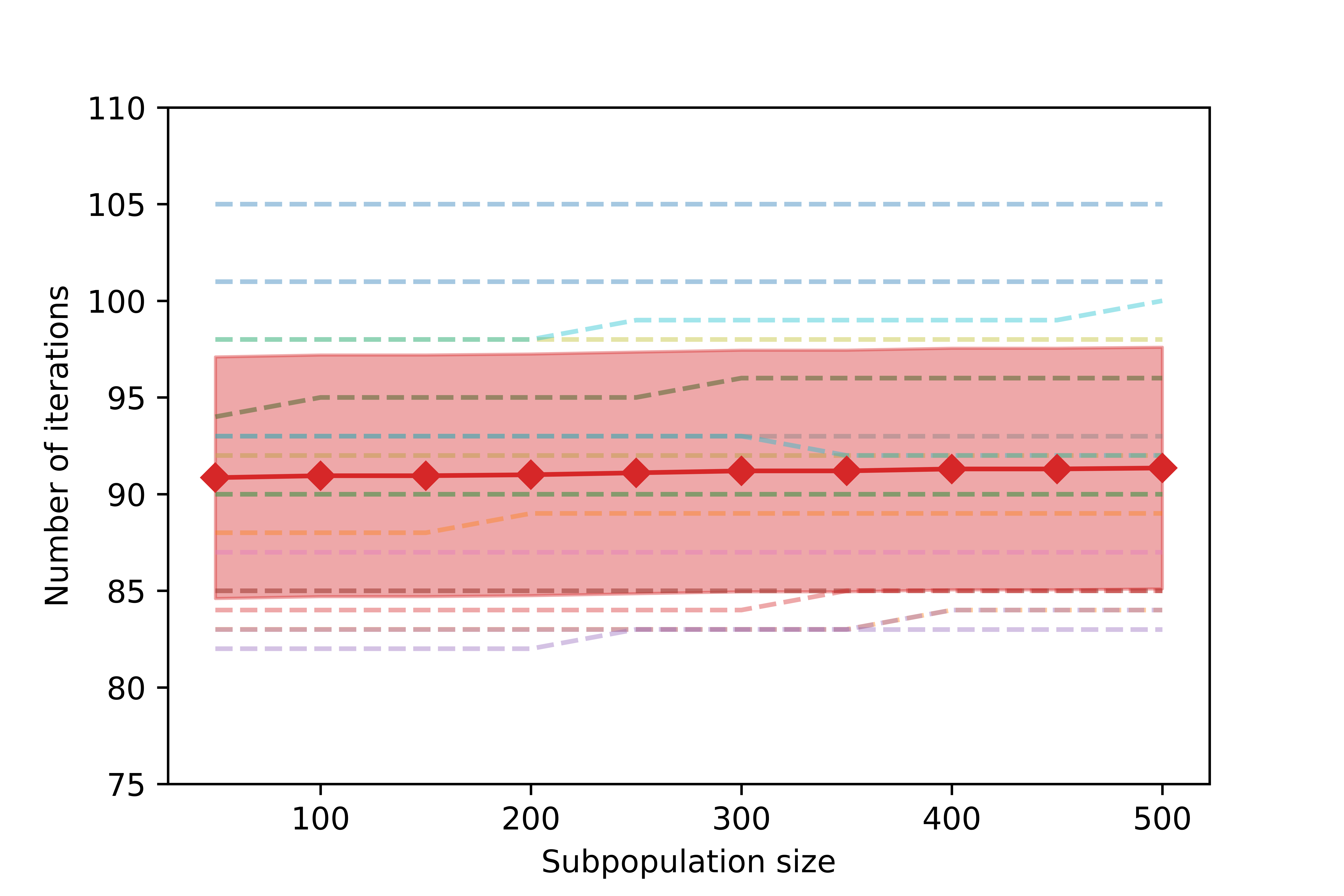
Figure 1: The number of iterations needed for the hierarchical natural actor-critic algorithm to converge to a predetermined precision as a function of the subpopulation size. Each dashed line represents the number of iterations of one simulated LQR instance. The red solid line represent the average number of iterations and the red shaded region indicates $1$-standard deviation. As the subpopulation size increases, the number of iterations needed are roughly fixed for all instances, validating that the computational complexity of the hierarchical natural actor-critic algorithm is independent of the number of agents in each subpopulation.

Acknowledgments

This work was completed in part with resources provided by the University of Chicago Research Computing Center.

A Policy Evaluation Algorithm

For completeness, we introduce a policy evaluation algorithm based on gradient-based temporal difference learning (Algorithm 2 in Yang et al. (2019)) that can be implemented in Algorithm 2.

In the LQR setting, the state- and action-value functions of policy $\pi_{K}$ take, respectively, the following forms

$$V_{K}(x)=\sum_{t=0}^{\infty}\left\{\mathbb{E}\left[c\left(x_{t},u_{t}\right)|x_{0}=x\right]-C(K)\right\},\quad Q_{K}(x,u)=c(x,u)-C(K)+\mathbb{E}_{x^{\prime}}\left[V_{K}\left(x^{\prime}\right)\right],$$ (54)

where $\{(x_{t},u_{t})\}_{t\geq 0}$ is the sequence of state-action pairs generated by policy $\pi_{K}$ with initial state $x_{0}=x$. Here we use $x^{\prime}$ to denote the next state generated by $(x,u)$, i.e. $x^{\prime}=Ax+Bu+w$, where the noise $w\sim N\left(0,\Phi\right)$ for some positive definite matrix $\Phi$.

The following lemma establishes the functional forms of the state- and action-value functions.

Lemma 6

The state and action value functions (54) are given, respectively, by

$$V_{K}(x) =x^{\top}P_{K}x-\mathop{\mathrm{tr}}\left(P_{K}\Sigma_{K}\right),$$ (55)

$$Q_{K}(x,u) =\varphi(v)^{\top}\delta_{K}^{*}-\sigma^{2}\cdot\mathop{\mathrm{tr}}(R+P_{K}BB^{\top})-\mathop{\mathrm{tr}}\left(P_{K}\Sigma_{K}\right),$$ (56)

where $v=\mathop{\text{vec}}(x,u)$ and $\varphi(v)=\mathop{\text{svec}}(vv^{\top})$. The vector $\delta_{K}^{*}$ is called value vector and is related to matrices $A$, $B$, $Q$, $R$ and matrix $P_{K}$ defined in Lemma 13. Moreover, $E_{K}$ can be recovered with $\delta_{K}^{*}$ and $K$. The explicit form of $\delta_{K}^{*}$ is given in the proof in §B.1.

By Lemma 6, estimating the action-value function $Q_{K}(x,u)$ is equivalent to estimating $\delta_{K}^{*}$ and thus gives estimator of $E_{K}$ as we desire.

Lemma 17 tells us that $v=[x^{\top},u^{\top}]^{\top}\sim N(0,\breve{\Sigma}_{K})$ is a Markov chain. Hereafter, we use $c(v)$ to denote $c(x,u)$. Similar notation is also used for other functions.

Note that $V_{K}(x)=\mathbb{E}_{u\sim\pi_{K}(\cdot|x)}\left[Q_{K}(v)\right]$, which indicates that for any $v\in\mathbb{R}^{d+k}$, we have

$$\left\langle\varphi(v),\delta_{K}^{*}\right\rangle=c(v)-C(K)+\left\langle\mathbb{E}\left[\varphi\left(v^{\prime}\right)\right],\delta_{K}^{*}\right\rangle,$$ (57)

where $v^{\prime}=\mathop{\text{vec}}\left(x^{\prime},u^{\prime}\right)$ is the next state-action pair generated by $v=\mathop{\text{vec}}(x,u)$. Denote the expectation with respect to $v\sim N(0,\breve{\Sigma}_{K})$ by $\mathbb{E}_{v}$. We let

$$b_{k}=(C(K)\ d_{K})^{\top},\ \Theta_{K}=\mathbb{E}_{v}\left\{\varphi(v)\left[\varphi(v)-\varphi\left(v^{\prime}\right)\right]^{\top}\right\},\text{ and }d_{K}=\mathbb{E}_{v}[c(v)\varphi(v)].$$

We also let $\gamma_{K}^{*}=\left(C(K),\delta_{K}^{*\top}\right)^{\top}$. It was shown in Yang et al. (2019) that $\left(\gamma_{K}^{*},0\right)^{\top}$ is the unique saddle point of the minimax optimization problem:

$$\min_{\gamma\in\mathcal{X}_{\Gamma}}\max_{\xi\in\mathcal{X}_{\Xi}}G(\gamma,\xi)=\left[\gamma^{1}-C(K)\right]\cdot\xi^{1}+\left\langle\gamma^{1}\cdot\mathbb{E}_{v}[\varphi(v)]+\Theta_{K}\gamma^{2}-d_{K},\xi^{2}\right\rangle-1/2\cdot\|\xi\|_{2}^{2},$$ (58)

where $\mathcal{X}_{\Gamma}$ and $\mathcal{X}_{\Xi}$ are compact sets and $\gamma=(\gamma^{1},\gamma^{2})$ and $\xi=(\xi^{1},\xi^{2})$ are primal and dual variables.

We solve (58) with stochastic gradient method, and return $\hat{\delta}_{K}=\hat{\gamma}^{2}$ as the estimator of $\delta_{K}^{*}$. Algorithm 3 details the Gradient-Based Temporal Difference (GTD) Algorithm.

To present the theoretical result of the policy evaluation algorithm using GTD, we make the following assumptions. First, we specify the compact sets $\mathcal{X}_{\Gamma}$ and $\mathcal{X}_{\Xi}$ defined in (58) to be

$$\mathcal{X}_{\Gamma} =\{\gamma:0\leq\gamma^{1}\leq\Gamma^{1},\|\gamma^{2}\|_{2}\leq\Gamma^{2}\},$$ (59)

$$\mathcal{X}_{\Xi} =\{\xi:0\leq|\xi^{1}|\leq\Xi^{1}=C(K_{0}),\|\xi^{2}\|_{2}\leq\Xi^{2}\},$$

where $\Gamma^{1}=C(K_{0})$, $\Gamma^{2}=\|Q\|_{{\mathrm{F}}}+\|R\|_{{\mathrm{F}}}+\sqrt{d}/\sigma_{\min}(\Phi)\cdot(\|A\|_{{\mathrm{F}}}^{2}+\|B\|_{{\mathrm{F}}}^{2})\cdot C(K_{0})$, $\Xi^{1}=C(K_{0})$, and $\Xi^{2}=C\cdot\left(1+\|K\|_{\mathrm{F}}^{2}\right)^{2}\cdot\Gamma^{2}\cdot\sigma_{\min}^{-2}(Q)\cdot[C(K_{0})]^{2}$. Here, $C$ is a constant that does not depend on $K$. Moreover, we set the step size in Algorithm 3 to be $\alpha_{t}=\alpha/\sqrt{t}$.

Algorithm 3 Gradient-Based Temporal-Difference (Algorithm 2 in Yang et al. (2019))

  Input: Current policy $\pi_{K}$, number of iterations $T$, and step sizes $\{\alpha_{t}=\alpha/\sqrt{t}\}_{t\in\{1,2,\dots,T\}}$.

  Initialization: Initialize $\gamma_{0}\in\mathcal{X}_{\Gamma}$ and $\xi_{0}\in\mathcal{X}_{\Xi}$. Sample the initial state-action pairs $x_{0}\sim\mathcal{D}_{K}$, $u_{0}\sim\pi_{K}\left(\cdot|x_{0}\right)$, and construct $v_{0}$. Observe the cost $c_{0}$ and the next state $x_{1}$.

  for $t=1,2,\ldots,T$ do

     Take action $u_{t}\sim\pi_{K}\left(\cdot|x_{t}\right)$ , set $v_{t}=\mathop{\text{vec}}(x_{t},u_{t})$, observe the cost $c_{t}$ and the next state $x_{t+1}$.

     Update primal-dual parameters $\gamma_{t-1}$ and $\xi_{t-1}$ with gradient decent to obtain $\gamma_{t}$ and $\xi_{t}$.

     Project $\gamma_{t}$ and $\xi_{t}$ to $\mathcal{X}_{\Gamma}$ and $\mathcal{X}_{\Xi}$.

  end for

  Obtain $\hat{\gamma}=(\hat{\gamma}^{1},\hat{\gamma}^{2})=(\sum_{t=1}^{T}\alpha_{t}\cdot\gamma_{t})/(\sum_{t=1}^{T}\alpha_{t})$ and $\hat{\xi}=(\sum_{t=1}^{T}\alpha_{t}\cdot\xi_{t})/(\sum_{t=1}^{T}\alpha_{t})$.

  Output: Estimators $\hat{C}=\hat{\gamma}^{1}$ of cost $C(K)$ and $\hat{\delta}_{K}=\hat{\gamma}^{2}$ of $\delta_{K}^{*}$.

Theorem 4 (Policy evaluation algorithm using GTD)

Let initial policy $\pi_{K_{0}}$ be stable in the sense that $\rho(A-BK_{0})<1$. Let $\mathcal{X}_{\Gamma}$ and $\mathcal{X}_{\Xi}$ be compact sets specified in (59). For any $\rho\in(\rho(A-BK),1)$, there exists sufficiently large iteration number $T$, so that with probability at least $1-T^{-4}$, we have

$$\|\hat{\delta}_{K}-\delta_{K}^{*}\|_{2}^{2}\leq\Lambda\left(\Gamma^{2},\Xi^{2},C(K_{0}),\|K\|_{\mathrm{F}},\Sigma_{K},\sigma_{\min}^{-1}(Q)\right)\cdot\frac{{\log^{6}T}}{(1-\rho){\tau_{K}^{*}}^{2}\sqrt{T}},$$ (60)

where $\Lambda$ is a polynomial of $\Gamma^{2}$, $\Xi^{2}$, $C(K_{0})$, $\|K\|_{\mathrm{F}}$, $\Sigma_{K}$ and $\sigma_{\min}^{-1}(Q)$, and constant ${\tau_{K}^{*}}>0$ solely depends on $\rho(A-BK)$, $\sigma$, and $\sigma_{\min}(\Phi)$.

A.1 Proof Sketch of Theorem 4

We will use Lemma 20 to establish the result. We start by verifying the conditions of Lemma 20. The following lemma shows that $(\gamma_{K}^{*},0)$ is the solution to the optimization problem (58).

Lemma 7

It holds that $\gamma_{K}^{*}\in\mathcal{X}_{\Gamma}$. Let $\xi(\gamma)$ be the solution to the unconstrained problem $\max_{\xi}G(\gamma,\xi)$. Then for any $\gamma\in\mathcal{X}_{\Gamma}$, we have $\xi(\gamma)\in\mathcal{X}_{\Xi}$.

Proof  See §B.2 for a detailed proof.  

For fixed values $\hat{\gamma}\in\Gamma$ and $\hat{\xi}\in\Xi$, we let

$$G_{\hat{\gamma}\cdot}=\max_{\xi\in\Xi}G(\hat{\gamma},\xi),\quad G_{\cdot\hat{\xi}}=\min_{\gamma\in\Gamma}G(\gamma,\hat{\xi}).$$

The primal-dual gap with respect to $\hat{\gamma}$ and $\hat{\xi}$ is defined as $G_{\hat{\gamma}\cdot}-G_{\cdot\hat{\xi}}$, which measures the closeness between $(\hat{\gamma},\hat{\xi})$ and the saddle point $(\delta_{K}^{*},0)$. The rate of convergence of the estimators obtained by the primal-dual problem (58) is controlled by the primal-dual gap $G_{\hat{\gamma}\cdot}-G_{\cdot\hat{\xi}}$ as shown by the following lemma.

Lemma 8

It holds that

$${\tau_{K}^{*}}^{2}\left(|\gamma^{1}-C(K)|^{2}+\|\hat{\delta}_{K}-\delta_{K}^{*}\|^{2}_{2}\right)\leq G_{\hat{\gamma}\cdot}-G_{\cdot\hat{\xi}},$$ (61)

where $\tau_{K}^{*}>0$ is a constant that depends only on $\rho(A-BK)$, $\sigma$, and $\sigma_{\min}(\Phi)$.

Proof  See §B.3 for a detailed proof.  

Next, we construct an upper bound on $G_{\hat{\gamma}\cdot}-G_{\cdot\hat{\xi}}$. For technical reasons, it is convenient to consider the case where $\|v_{t}\|^{2}=\left\|x_{t}\right\|_{2}^{2}+\left\|u_{t}\right\|_{2}^{2}$ is bounded by some value that depends on $T$, for $0\leq t\leq T$. This will guarantee better Lipschitz properties of $G(\gamma,\xi)$ and thus enable us to bound the primal-dual gap. We use the following lemma to characterize the tail distribution of $v$.

Lemma 9

Consider the event

$$\mathcal{A}=\left\{\|v\|_{2}^{2}-\mathop{\mathrm{tr}}\left(\breve{\Sigma}_{K}\right)\leq C^{\prime}\cdot\log T\cdot\|\breve{\Sigma}_{K}\|\right\},$$

where $v\sim N(0,\breve{\Sigma}_{K})$ and $\breve{\Sigma}_{K}$ is defined in Lemma 17. We have $\mathbb{P}(\mathcal{A}^{c})\leq T^{-6}$ when $C^{\prime}$ is large enough.

Proof  See §B.4 for a detailed proof.  

Hereafter, we consider the optimization problem in (58) conditioned on event $\mathcal{A}$ defined in Lemma 9. Define the truncated feature vector by $\tilde{\varphi}(v)=\varphi(v)\cdot\operatorname{\mathds{1}}_{\mathcal{A}}$. Let $\tilde{\Theta}_{K}$ and $\tilde{d}_{K}$ be defined as $\Theta_{K}$ and $d_{K}$, but with $\varphi(v)$ and $\varphi(v^{\prime})$ replaced with $\tilde{\varphi}(v)$ and $\tilde{\varphi}(v^{\prime})$, respectively. Consider the new optimization problem

$$\min_{\gamma\in\mathcal{X}_{\Gamma}}\max_{\xi\in\mathcal{X}_{\Xi}}\tilde{G}(\gamma,\xi)=\left[\gamma^{1}-C(K)\right]\cdot\xi^{1}+\left\langle\gamma^{1}\cdot\mathbb{E}_{v}[\tilde{\varphi}(v)]+\tilde{\Theta}_{K}\gamma^{2}-\tilde{d}_{K},\xi^{2}\right\rangle-1/2\cdot\|\xi\|_{2}^{2}.$$ (62)

For sufficiently large $T$, the objectives in (58) and (62) are close.

Lemma 10

When $T$ is sufficiently large, it holds that

$$|G(\gamma,\xi)-\widetilde{G}(\gamma,\xi)|\leq\frac{1}{T}$$ (63)

for any $\gamma\in\mathcal{X}_{\Gamma}$, $\xi\in\mathcal{X}_{\Xi}$.

Proof  See §B.5 for a detailed proof.  

A direct corollary is that the difference of primal-dual gaps between optimization problems (58) and (62) can be bounded as

$$|(G_{\hat{\gamma}\cdot}-G_{\cdot\hat{\xi}})-(\tilde{G}_{\hat{\gamma}\cdot}-\tilde{G}_{\cdot\hat{\xi}})|\leq\frac{2}{T}.$$ (64)

The objective function of the truncated optimization problem (62) has good properties as characterized by the following lemma.

Lemma 11

As a function of $\gamma$ and $\xi$, the norm of $\nabla\tilde{G}(\gamma,\xi)$ can be bounded by

$$3(\Gamma^{2}+\Xi^{2})\cdot(C^{\prime}\cdot\log T+d+k)^{2}[\sigma^{2}+(1+\|K\|_{F}^{2})\|\Sigma_{K}\|]^{2}=:L_{1},$$ (65)

for a sufficiently large $C^{\prime}$. Thus, $\widetilde{G}(\gamma,\xi)$ is Lipschitz for both $\gamma$ and $\xi$ with finite a constant $L_{1}$. Moreover, we have $\nabla^{2}_{\gamma\gamma}\tilde{G}(\gamma,\xi)=0$ and $\nabla^{2}_{\xi\xi}\tilde{G}(\gamma,\xi)=-I$, where $I$ is the identity matrix of proper dimension.

Proof  See §B.6 for a detailed proof.  

Finally, Lemma 17 shows that $\{v_{t}\}_{t\geq 0}$ is a geometrically $\beta$-mixing stochastic process with a parameter $\rho\in(\rho(A-BK),1)$ and thus mixes rapidly. Therefore, we have verified the conditions of Lemma 20, which gives an upper bound on the primal-dual gap in (62). We have the following result.

Lemma 12

For a sufficiently large $T$, we have

$$\tilde{G}_{\hat{\gamma}\cdot}-\tilde{G}_{\cdot\hat{\xi}}\leq\Lambda_{3}\frac{{\log^{2}T}+\log(T^{5})}{\log(1/\rho)\cdot\sqrt{T}}+\Lambda_{4}\frac{\log^{6}T}{(1-\rho)T},$$ (66)

with probability at least $1-T^{-5}$, where $\Lambda_{3}$ and $\Lambda_{4}$ are polynomials of $\Gamma^{2}$, $\Xi^{2}$, $C(K_{0})$, $\|K\|_{\mathrm{F}}$, $\Sigma_{K}$, and $\sigma_{\min}^{-1}(Q)$.

Proof  See §B.7 for a detailed proof.  

Recall that for the event $\mathcal{A}_{t}=\left\{\|v_{t}\|_{2}^{2}-\mathop{\mathrm{tr}}\left(\breve{\Sigma}_{K}\right)>C^{\prime}\cdot\log T\cdot\left\|\breve{\Sigma}_{K}\right\|\right\}$, we have $P(\mathcal{A})\leq T^{-6}$ for $C_{1}$ large enough. Then the event $\bigcap_{t=1}^{T}\mathcal{A}_{t}$ holds with probability at least $1-T^{-5}$. Combining (66) and (64), it holds with probability at least $1-2T^{-5}>1-T^{-4}$ that the primal-dual gap of the original optimization problem 58 can be bounded as

$$G_{\hat{\gamma}\cdot}-G_{\cdot\hat{\xi}}\leq\Lambda_{3}\frac{{\log^{2}T}+\log(T^{5})}{\log(1/\rho)\cdot\sqrt{T}}+\Lambda_{4}\frac{\log^{6}T}{(1-\rho)T}+\frac{2}{T}.$$ (67)

The formula above is dominated by the first term on the right-hand side. Combining (67) and Lemma (61), we establish Theorem 4.

B Technical Proofs of Lemmas in §A.1

B.1 Proof of Lemma 6

Since the dynamic is linear, $V_{K}(x)$ has a quadratic form in $x$ specified as

$$V_{K}(x) =\sum_{t=0}^{\infty}\left\{\mathbb{E}\left[c\left(x_{t},u_{t}\right)|x_{0}=x\right]-C(K)\right\}$$

$$=\sum_{t=0}^{\infty}\left\{\mathbb{E}\left[x_{t}^{\top}\left(Q+K^{\top}RK\right)x_{t}\right]+\sigma^{2}\cdot\mathop{\mathrm{tr}}(R)-C(K)\right\}.$$ (68)

By definition, we have $E_{x\sim\mathcal{D}_{K}}[V_{K}(x)]=0$, so $V_{k}(x)=x^{\top}P_{K}x-E_{x\sim\mathcal{D}_{K}}\left[x^{\top}P_{K}x\right]$, for some matrix $P_{K}\in{}^{d\times d}$. We also have

$$V_{K}(x)=\mathbb{E}_{u\sim\pi_{K}}[c(x,u)]-C(K)+\mathbb{E}_{x^{\prime}}\left[V_{K}\left(x^{\prime}\right)\right],$$ (69)

where $x^{\prime}$ is the next state generated by $(x,u)$. Therefore, we find that $P_{K}$ is a solution to the equation

$$x^{\top}P_{K}x=x\left(Q+K^{\top}RK\right)x+x^{\top}(A-BK)^{\top}P_{K}(A-BK)x$$ (70)

and the functional form of $V_{K}(x)$ follows from computing

$$\mathbb{E}_{x\sim\mathcal{D}_{K}}\left[x^{\top}P_{K}x\right] =\mathop{\mathrm{tr}}\left[(Q+K^{\top}RK)\Sigma_{K}\right]+\mathop{\mathrm{tr}}\left[(A-BK)^{\top}P_{K}(A-BK)\Sigma_{K}\right]$$

$$=\mathop{\mathrm{tr}}\left[P_{K}\Phi_{\sigma}\right]+\mathop{\mathrm{tr}}\left[P_{K}(A-BK)\Sigma_{K}(A-BK)^{\top}\right]$$

$$=\mathop{\mathrm{tr}}\left(P_{K}\Sigma_{K}\right).$$ (71)

Direct computation yields the functional form of $Q_{K}(x,u)$:

$$Q_{K}(x,u) =c(x,u)-C(K)+\mathbb{E}_{x^{\prime}}\left[V_{K}\left(x^{\prime}\right)|x\right]$$

$$=x^{\top}Qx+u^{\top}Ru+(Ax+Bu)^{\top}P_{K}(Ax+Bu)+\mathop{\mathrm{tr}}\left(P_{K}\Phi\right)-C(K)-\mathop{\mathrm{tr}}\left(P_{K}\Sigma_{K}\right)$$

$$=v\top\Delta_{K}v-\sigma^{2}\cdot\mathop{\mathrm{tr}}(R+P_{K}BB^{\top})-\mathop{\mathrm{tr}}\left(P_{K}\Sigma_{K}\right),$$ (72)

where the last equation follows from (2), $\Phi_{\sigma}=\Phi+\sigma^{2}\cdot BB^{\top}$, and the matrix $\Delta_{K}$ is given by

$$\Delta_{K}=\left(\begin{array}[]{cc}{\Delta_{K}^{11}}&{\Delta_{K}^{12}}\\ {\Delta_{K}^{21}}&{\Delta_{K}^{22}}\end{array}\right)=\left(\begin{array}[]{cc}{Q+A^{\top}P_{K}A}&{A^{\top}P_{K}B}\\ {B^{\top}P_{K}A}&{R+B^{\top}P_{K}B}\end{array}\right).$$ (73)

We define $\delta_{K}^{*}=\operatorname{svec}(\Delta_{K})$. Then $\Delta_{K}$ can be recovered by $\Delta_{K}=\operatorname{smat}(\delta_{K}^{*})$. We can check that $E_{K}=\Delta_{K}^{22}K-\Delta_{K}^{21}$, thus estimating $\delta_{K}^{*}$ is equivalent to estimating $E_{K}$.

B.2 Proof of Lemma 7

To prove $\gamma_{K}^{*}\in\mathcal{X}_{\Gamma}$, we just need to show $\|\delta_{K}^{*}\|_{2}=\|\Delta_{K}\|_{F}\leq\Gamma^{2}$. Note that we have

$$\Delta_{K}=\left(\begin{array}[]{cc}{Q+A^{\top}P_{K}A}&{A^{\top}P_{K}B}\\ {B^{\top}P_{K}A}&{R+B^{\top}P_{K}B}\end{array}\right)={\rm diag}(Q,R)+\left(A\quad B\right)^{\top}P_{K}\left(A\quad B\right).$$ (74)

We have $\|\Delta_{K}\|_{\mathrm{F}}\leq\Gamma^{2}\leq\|Q\|_{\mathrm{F}}+\|R\|_{\mathrm{F}}+(\|A\|_{\mathrm{F}}^{2}+\|B\|_{\mathrm{F}}^{2})\cdot\|P_{K}\|_{\mathrm{F}}$. From Lemma 16, we have $\left\|P_{K}\right\|\leq C(K)/\sigma_{\min}(\Phi)$. Therefore, it holds that

$$\left\|P_{K}\right\|_{F}\leq\sqrt{d}/\sigma_{\min}(\Phi)\cdot C(K)\leq\sqrt{d}/\sigma_{\min}(\Phi)\cdot C(K_{0}).$$

Hence, we conclude

$$\|\Delta_{K}\|\leq\Gamma^{2} \leq\|Q\|_{\mathrm{F}}+\|R\|_{\mathrm{F}}+(\|A\|_{\mathrm{F}}^{2}+\|B\|_{\mathrm{F}}^{2})\cdot\|P_{K}\|_{\mathrm{F}}$$

$$\leq\|Q\|_{\mathrm{F}}+\|R\|_{\mathrm{F}}+(\|A\|_{\mathrm{F}}^{2}+\|B\|_{\mathrm{F}}^{2})\cdot\sqrt{d}/\sigma_{\min}(\Phi)\cdot C(K_{0}),$$ (75)

and thus we have $\gamma_{K}^{*}\in\mathcal{X}_{\Gamma}$.

To prove the second statement, observe that $\xi(\gamma)$ has components

$$\xi(\gamma)^{1} =\gamma^{1}-C(K),$$

$$\xi(\gamma)^{2} =\gamma^{1}\cdot\mathbb{E}_{v}[\varphi(v)]+\Theta_{K}\gamma^{2}-d_{K}.$$

We bound $|\gamma^{1}-C(K)|$, $\|\gamma^{1}\cdot\mathbb{E}_{(x,u)}[\varphi(v)]\|_{2}$, $\|\Theta_{K}\gamma^{2}\|_{2}$ and $\|d_{K}\|_{2}$ separately. From the fact that $0\leq\gamma^{1}\leq\Gamma^{1}=C\left(K_{0}\right)$, we have $|\gamma^{1}-C(K)|\leq C\left(K_{0}\right)$ and $0\leq|\xi^{1}|\leq\Xi^{1}$. From Lemma 17, we have

$$\|\gamma^{1}\cdot\mathbb{E}_{v}[\varphi(x,u)]\|_{2}\leq C(K_{0})\|\breve{\Sigma}_{K}\|_{\mathrm{F}}\leq C(K_{0})\left[k\sigma^{2}+(d+\|K\|_{\mathrm{F}}^{2})\cdot\left\|\Sigma_{K}\right\|\right].$$ (76)

From Lemma 19, we have $\|\Theta_{K}\gamma^{2}\|_{2}\leq\|\Theta_{K}\|\|\gamma^{2}\|_{2}\leq 4\left(1+\|K\|_{\mathrm{F}}^{2}\right)^{2}\cdot\left\|\Sigma_{K}\right\|^{2}\cdot\Gamma^{2}$. To bound $\|d_{K}\|_{2}$, note that for any positive definite matrix $\Sigma^{\prime}$, we can rewrite $d_{K}^{\top}\operatorname{svec}(\Sigma^{\prime})$ by

$$d_{K}^{\top}\operatorname{svec}(\Sigma^{\prime}) =\mathbb{E}_{v}\{\langle\phi(v),\operatorname{smat}[\operatorname{diag}(Q,R)]\rangle\cdot\langle\phi(v),\operatorname{smat}(\Gamma)\rangle$$

$$=2\left\langle\breve{\Sigma}_{K}\operatorname{diag}(Q,R)\breve{\Sigma}_{K},\Gamma\right\rangle\cdot\left\langle\breve{\Sigma}_{K},\operatorname{diag}(Q,R)\right\rangle\cdot\left\langle\breve{\Sigma}_{K},\Gamma\right\rangle,$$ (77)

where the second equation follows from Lemma 22 and $\breve{\Sigma}_{K}$ is defined in Lemma 17. Thus, we conclude $\left\|d_{K}\right\|_{2}\leq 3\left(\|Q\|_{\mathrm{F}}+\|R\|_{\mathrm{F}}\right)\cdot\left\|\breve{\Sigma}_{K}\right\|^{2}$. Combining the bounds above and (5.6), we conclude that for some constant $C$,

$$\left\|\xi^{2}\right\|_{2} \leq C(K_{0})\left[k\sigma^{2}+(d+\|K\|_{\mathrm{F}}^{2})\cdot\left\|\Sigma_{K}\right\|\right]+4\left(1+\|K\|_{\mathrm{F}}^{2}\right)^{2}\cdot\left\|\Sigma_{K}\right\|^{2}\cdot\Gamma^{2}$$

$$\quad+12\left(\|Q\|_{\mathrm{F}}+\|R\|_{\mathrm{F}}\right)\cdot\left(d+\|K\|_{\mathrm{F}}^{2}\right)^{2}\cdot\left\|\Sigma_{K}\right\|^{2}$$

$$\leq C\cdot\left(1+\|K\|_{\mathrm{F}}^{2}\right)^{2}\cdot\Gamma^{2}\cdot\sigma_{\min}^{-2}(Q)\cdot[C(K_{0})]^{2}.$$ (78)

B.3 Proof of Lemma 8

Note that the optimal value of the dual problem satisfies

$$G_{\hat{\gamma}\cdot}=\max_{\xi\in\mathcal{X}_{\Xi}}G(\hat{\gamma},\xi) =\|\widehat{\gamma}^{1}-C(K)\|^{2}+\left\|\widehat{\gamma}^{1}\cdot\mathbb{E}_{(x,u)}[\varphi(x,u)]+\Theta_{K}\hat{\gamma}^{2}-d_{K}\right\|_{2}^{2}$$

$$=\|\Omega_{K}\hat{\gamma}-b_{K}\|_{2}^{2}=\|\Omega_{K}(\hat{\gamma}-\gamma_{K}^{*})\|_{2}^{2},$$ (79)

where we define

$$\Omega_{K}=\left(\begin{array}[]{cc}{1}&{0}\\ {\mathbb{E}_{v}[\varphi(v)]}&{\Theta_{K}}\end{array}\right),\quad\gamma_{K}^{*}=\left(C(K),\delta_{K}^{*\top}\right)^{\top}.$$ (80)

The optimal value of the primal value satisfies

$$G_{\cdot\hat{\xi}}=\min_{\gamma\in\mathcal{X}_{\Gamma}}G(\gamma,\hat{\xi})\leq\min_{\gamma\in\mathcal{X}_{\Gamma}}G_{\hat{\gamma}\cdot}=\min_{\gamma\in\mathcal{X}_{\Gamma}}\|\Omega_{K}\hat{\gamma}-b_{K}\|_{2}^{2}=0.$$ (81)

Therefore $\|\Omega_{K}(\hat{\gamma}-\gamma_{K}^{*})\|_{2}^{2}\leq G_{\hat{\gamma}\cdot}-G_{\cdot\hat{\xi}}$. Moreover, by Lemma 19, we have $\|\Omega_{K}\|\geq\tau_{K}^{*}>0$ for some constant $\tau_{K}^{*}$ that only depends on $\rho(A-BK)$, $\sigma$, and $\sigma_{\min}(\Phi)$. Hence, we have

$$(\tau_{K}^{*})^{2}\left(|\gamma^{1}-C(K)|^{2}+\|\hat{\Delta}_{K}-\Delta_{K}\|^{2}_{F}\right)\leq\tau_{K}^{*}\|\hat{\gamma}-(\tau_{K}^{*})^{2}\|_{2}^{2}\leq\|\Omega_{K}(\hat{\gamma}-\gamma_{K}^{*})\|_{2}^{2}\leq G_{\hat{\gamma}\cdot}-G_{\cdot\hat{\xi}}.$$ (82)

B.4 Proof of Lemma 9

Set $s=C^{\prime}\cdot\log T\cdot\left\|\breve{\Sigma}_{K}\right\|$ with $C^{\prime}$ sufficiently large so that $s^{2}\cdot\|\breve{\Sigma}_{K}\|_{\mathrm{F}}^{-2}\geq s\cdot\|\breve{\Sigma}_{K}\|^{-1}$. Applying Lemma 18 to $v\sim N\left(0,\breve{\Sigma}_{K}\right)$, we get

$$\mathbb{P}\left[\|v\|_{2}^{2}-\mathop{\mathrm{tr}}(\breve{\Sigma}_{K})|>s\right] \leq 2\cdot\exp[-C\cdot\min(s^{2}\cdot\|\breve{\Sigma}_{K}\|_{\mathrm{F}}^{-2},s\cdot\|\breve{\Sigma}_{K}\|^{-1})]$$

$$=2\cdot\exp[-C\cdot\|\breve{\Sigma}_{K}\|^{-1}\cdot s]$$

$$=2\cdot\exp[-C\cdot C^{\prime}\cdot\log T].$$ (83)

When $C^{\prime}$ is sufficiently large, we have $\mathbb{P}\left(\mathcal{A}^{c}\right)\leq T^{-6}$.

B.5 Proof of Lemma 10

By direct computation, we have

$$G(\gamma,\xi)-\widetilde{G}(\gamma,\xi) =\left[\gamma^{1}-\mathbb{E}_{v}[c(v)]\right]\cdot\xi^{1}-\left[\gamma^{1}-\mathbb{E}_{v}[c(v)\cdot\operatorname{\mathds{1}}_{\mathcal{A}}]\right]\cdot\xi^{1}$$

$$\quad+\left\langle\gamma^{1}\cdot\mathbb{E}_{v}[\varphi(v)]+\Theta_{K}\gamma^{2}-d_{K},\xi^{2}\right\rangle-\left\langle\gamma^{1}\cdot\mathbb{E}_{v}[\tilde{\varphi}(v)]+\tilde{\Theta}_{K}\gamma^{2}-\tilde{d}_{K},\xi^{2}\right\rangle$$

$$=\mathbb{E}_{v}\left[c(v)\cdot\operatorname{\mathds{1}}_{\mathcal{A}^{c}}\right]\cdot\xi^{1}-\left\langle\mathbb{E}_{v}\left[\varphi(v)\varphi(v^{\prime})^{\top}\operatorname{\mathds{1}}_{\mathcal{A}}\operatorname{\mathds{1}}_{\mathcal{A^{\prime}}^{c}}\right]\gamma^{2},\xi^{2}\right\rangle$$

$$\quad+\left\langle\mathbb{E}_{v}\left[\gamma^{1}\cdot\varphi(v)\operatorname{\mathds{1}}_{\mathcal{A}^{c}}+\varphi(v)[\varphi(v)-\varphi(v^{\prime})]^{\top}\operatorname{\mathds{1}}_{\mathcal{A}^{c}}\gamma^{2}-c(v)\varphi(v)\operatorname{\mathds{1}}_{\mathcal{A}^{c}}\right],\xi^{2}\right\rangle$$

$$=\mathbb{E}_{v}\left[c(v)\cdot\operatorname{\mathds{1}}_{\mathcal{A}^{c}}\right]\cdot\xi^{1}-\left\langle\mathbb{E}_{v}\left[\varphi(v)\varphi(v^{\prime})^{\top}\operatorname{\mathds{1}}_{\mathcal{A}}\operatorname{\mathds{1}}_{\mathcal{A^{\prime}}^{c}}\right]\gamma^{2},\xi^{2}\right\rangle$$

$$\quad+\left\langle\mathbb{E}_{v}\left[\varphi(v)[\gamma^{1}-c(v)+\varphi(v)^{\top}\gamma^{2}]\operatorname{\mathds{1}}_{\mathcal{A}^{c}}-\varphi(v)\varphi(v^{\prime})^{\top}\gamma^{2}\operatorname{\mathds{1}}_{\mathcal{A}^{c}}\right],\xi^{2}\right\rangle$$ (84)

and

$$|G(\gamma,\xi)-\widetilde{G}(\gamma,\xi)| \leq\left|\mathbb{E}_{v}\left[c(v)\cdot\operatorname{\mathds{1}}_{\mathcal{A}^{c}}\right]\right|\cdot C\left(K_{0}\right)+\left\|\mathbb{E}_{v}\left[\varphi(v)\varphi(v^{\prime})^{\top}\operatorname{\mathds{1}}_{\mathcal{A}}\operatorname{\mathds{1}}_{\mathcal{A^{\prime}}^{c}}\right]\gamma^{2}\right\|\cdot\Xi^{2}$$

$$\quad+\left\|\mathbb{E}_{v}\left[\gamma^{1}\cdot\varphi(v)\operatorname{\mathds{1}}_{\mathcal{A}^{c}}+\varphi(v)[\varphi(v)-\varphi(v^{\prime})]^{\top}\operatorname{\mathds{1}}_{\mathcal{A}^{c}}\gamma^{2}-c(v)\varphi(v)\operatorname{\mathds{1}}_{\mathcal{A}^{c}}\right]\right\|\cdot\Xi^{2}.$$ (85)

We can bound each term on the right-hand side separately with

$$\left(\left|\mathbb{E}_{v}\left[c(v)\cdot\operatorname{\mathds{1}}_{\mathcal{A}^{c}}\right]\right|\leq\mathbb{E}\left[c^{2}(v)\right]\right)^{\frac{1}{2}}\cdot\mathbb{P}\left(\mathcal{A}^{c}\right)^{\frac{1}{2}},$$ (86)

$$\left\|\mathbb{E}_{v}\left[\varphi(v)\varphi(v^{\prime})^{\top}\operatorname{\mathds{1}}_{\mathcal{A}}\operatorname{\mathds{1}}_{\mathcal{A^{\prime}}^{c}}\right]\gamma^{2}\right\|\leq\left(\mathbb{E}_{v}\left[\|\varphi(v)\varphi(v^{\prime})^{\top}\|^{2}_{2}\right]\right)^{\frac{1}{2}}\cdot\mathbb{P}\left(\mathcal{A}^{c}\right)^{\frac{1}{2}},$$ (87)

where

$$\mathbb{E}_{v}\left[\|\varphi(v)\varphi(v^{\prime})^{\top}\gamma^{2}\|^{2}_{2}\right]\leq\left(\mathbb{E}\left[|\varphi\left(v^{\prime}\right)^{\top}\gamma^{2}|^{4}\right]\cdot\mathbb{E}\left[\|\varphi(v)\|_{2}^{4}\right]\right)^{\frac{1}{2}}.$$ (88)

Furthermore,

$$\left\|\mathbb{E}_{v}\left[\varphi(v)[\gamma^{1}-c(v)+\varphi(v)^{\top}\gamma^{2}]\operatorname{\mathds{1}}_{\mathcal{A}^{c}}-\varphi(v)\varphi(v^{\prime})^{\top}\gamma^{2}\operatorname{\mathds{1}}_{\mathcal{A}^{c}}\right]\right\|$$

$$\qquad\leq\left(\mathbb{E}_{v}\left[\left\|\varphi(v)[\gamma^{1}-c(v)+\varphi(v)^{\top}\gamma^{2}]-\varphi(v)\varphi(v^{\prime})^{\top}\gamma^{2}\right\|^{2}\right]\right)^{\frac{1}{2}}\cdot\mathbb{P}\left(\mathcal{A}^{c}\right)^{\frac{1}{2}},$$ (89)

where

$$\mathbb{E}_{v}\left[\left\|\varphi(v)[\gamma^{1}-c(v)+\varphi(v)^{\top}\gamma^{2}]-\varphi(v)\varphi(v^{\prime})^{\top}\gamma^{2}\right\|^{2}\right]$$

$$\leq 2\mathbb{E}_{v}\left[\left|\gamma^{1}-c(v)+\varphi(v)^{\top}\gamma^{2}\right|^{2}\left\|\varphi(v)\right\|^{2}+\left\|\varphi(v)\varphi(v^{\prime})^{\top}\gamma^{2}\right\|^{2}\right]$$

$$\leq 2\left(\mathbb{E}_{v}\left[|\gamma^{1}-c(v)+\varphi(v)^{\top}\gamma^{2}|^{4}\right]\cdot\mathbb{E}_{v}\left[\left\|\varphi(v)\right\|^{4}\right]\right)^{\frac{1}{2}}+2\left(\mathbb{E}_{v}\left[|\varphi\left(v^{\prime}\right)^{\top}\gamma^{2}|^{4}\right]\cdot\mathbb{E}_{v}\left[\|\varphi(v)\|_{2}^{4}\right]\right)^{\frac{1}{2}}.$$ (90)

Note that (88) and (B.5) can be bounded by the fourth moments of $N\left(0,\breve{\Sigma}_{K}\right)$. Since $P(\mathcal{A}^{c})\leq T^{-6}$, when $T$ is sufficiently large, it holds that $|G(\gamma,\xi)-\widetilde{G}(\gamma,\xi)|\leq 1/T$.

B.6 Proof of Lemma 11

By direct computation, we have

$$\nabla_{\gamma^{1}}G\left(\gamma,\xi\right) =\xi^{1}+\mathbb{E}_{v}[\widetilde{\varphi}(v)^{\top}]\xi^{2},$$ (91)

$$\nabla_{\gamma^{2}}G\left(\gamma,\xi\right) =\mathbb{E}_{v}\left[\widetilde{\varphi}(v)^{\top}\xi^{2}\cdot[\widetilde{\varphi}(v)-\widetilde{\varphi}\left(v^{\prime}\right)]\right],$$ (92)

$$\nabla_{\xi^{1}}G\left(\gamma,\xi\right) =\gamma^{1}-\mathbb{E}_{v}[\widetilde{c}(v)]-\xi^{1},$$ (93)

$$\nabla_{\xi^{2}}G\left(\gamma,\xi\right) =\mathbb{E}_{v}\left[\gamma^{1}\widetilde{\varphi}(v)+\widetilde{\varphi}(v)(\widetilde{\varphi}(v)-\widetilde{\varphi}(v^{\prime}))^{\top}\gamma^{2}-\widetilde{c}(v)\widetilde{\varphi}(v)\right]-\xi^{2}.$$ (94)

By definition, we have the bound

$$\|\tilde{\varphi}(v)\|_{2} \leq C^{\prime}\cdot\log T\cdot\|\breve{\Sigma}_{K}\|+\mathop{\mathrm{tr}}(\breve{\Sigma}_{K})$$

$$\leq(C^{\prime}\cdot\log T+d+k)\|\breve{\Sigma}_{K}\|$$

$$\leq(C^{\prime}\cdot\log T+d+k)[\sigma^{2}+(1+\|K\|_{F}^{2})\|\Sigma_{K}\|],$$ (95)

where the last inequality follows from (136). The same bound holds for $\|\tilde{\varphi}(v^{\prime})\|_{2}$.

Combining (B.6) and definitions of $\mathcal{X}_{\Gamma}$ and $\mathcal{X}_{\Xi}$, by direct computation, we have

$$\|\nabla_{\gamma}\widetilde{G}(\gamma,\xi)\|_{2} \leq C(K_{0})+\|\widetilde{\varphi}(v)\|_{2}\cdot\|\xi^{2}\|_{2}+\|\widetilde{\varphi}(v)\|_{2}\cdot\|\xi^{2}\|_{2}\cdot\|\tilde{\varphi}(v)+\tilde{\varphi}(v^{\prime})\|_{2}$$

$$\leq C(K_{0})+\Xi^{2}\cdot(C^{\prime}\cdot\log T+d+k)[\sigma^{2}+(1+\|K\|_{F}^{2})\|\Sigma_{K}\|]$$

$$\quad+2\cdot\Xi^{2}\cdot(C^{\prime}\cdot\log T+d+k)^{2}[\sigma^{2}+(1+\|K\|_{F}^{2})\|\Sigma_{K}\|]^{2}.$$ (96)

Similarly, we have

$$\|\nabla_{\xi}\widetilde{G}(\gamma,\xi)\|_{2} \leq 2C(K_{0})+C(K_{0})(C^{\prime}\cdot\log T+d+k)[\sigma^{2}+(1+\|K\|_{F}^{2})\|\Sigma_{K}\|]$$

$$\quad+2\cdot\Gamma^{2}\cdot(C^{\prime}\cdot\log T+d+k)^{2}[\sigma^{2}+(1+\|K\|_{F}^{2})\|\Sigma_{K}\|]^{2}\cdot$$

$$\quad+C(K_{0})(C^{\prime}\cdot\log T+d+k)[\sigma^{2}+(1+\|K\|_{F}^{2})\|\Sigma_{K}\|]+\Xi^{2}.$$ (97)

Using that fact that $\sqrt{x+y}<x+y$ when $x>0$ and $y>0$, we have

$$\|\nabla\widetilde{G}(\gamma,\xi)\|_{2} \leq\|\nabla_{\gamma}\widetilde{G}(\gamma,\xi)\|_{2}+\|\nabla_{\xi}\widetilde{G}(\gamma,\xi)\|_{2}$$

$$\leq 3(\Gamma^{2}+\Xi^{2})\cdot(C^{\prime}\cdot\log T+d+k)^{2}[\sigma^{2}+(1+\|K\|_{F}^{2})\|\Sigma_{K}\|]^{2},$$ (98)

where $C_{1}$ is sufficiently large.

B.7 Proof of Lemma 12

We can further specify $L_{1}$, $L_{2}$, $D$ and $C_{\zeta}$. By Lemma 11, we can set

$$L_{1}=3(\Gamma^{2}+\Xi^{2})\cdot(C^{\prime}\cdot\log T+d+k)^{2}[\sigma^{2}+(1+\|K\|_{F}^{2})\|\Sigma_{K}\|]^{2},\quad L_{2}=1.$$ (99)

By (59), we can set $D$ to be

$$D=(2C(K_{0})^{2}+(\Gamma^{2})^{2}+(\Xi^{2})^{2})^{1/2}.$$ (100)

By Lemma 17 and 21, we can set

$$C_{\zeta}=C_{\rho,\breve{K}}\cdot\left[\mathop{\mathrm{tr}}\left(\breve{\Sigma}_{K}\right)+(d+k)\cdot(1-\rho)^{-2}\right]^{1/2}.$$ (101)

Set $\delta=T^{-5}$ and note that $\log x<x+1$ for $\forall x>0$. We conclude that with probability at least $1-T^{-5}$ the primal-dual gap conditioned on $\bigcap_{t=1}^{T}\mathcal{A}_{t}$ is bounded by

$$\tilde{G}_{\hat{\gamma}\cdot}-\tilde{G}_{\cdot\hat{\xi}}\leq\Lambda_{3}\frac{{\log^{2}T}+\log(T^{5})}{\log(1/\rho)\cdot\sqrt{T}}+\Lambda_{4}\frac{\log^{6}T}{(1-\rho)T},$$ (102)

when $T$ is sufficiently large, where $\Lambda_{3}$ and $\Lambda_{4}$ are polynomials of $\Gamma^{2}$, $\Xi^{2}$, $C(K_{0})$, $\|K\|_{\mathrm{F}}$, $\Sigma_{K}$, and $\sigma_{\min}^{-1}(Q)$ .

C Proof of Supporting Lemmas

In this section, we lay out the proofs of supporting lemmas.

Lemma 13

Consider the LQR problem specified by

$$x_{t+1}=Ax_{t}+Bu_{t}+w_{t},\quad c\left(x_{t},u_{t}\right)=x_{t}^{\top}Qx_{t}+u_{t}^{\top}Ru_{t},$$ (103)

where $A$, $B$, $Q$ and $R$ are matrices of proper dimensions, and noise $w_{t}\sim N(0,\Phi)$, with matrices $Q,R,\Phi\succ 0$. Under a policy $\pi_{K}$ that satisfies $\rho(A-BK)<1$, an action $u_{t}$ is written as $-Kx_{t}+\sigma\cdot z_{t}$, where $z_{t}\sim N\left(0,I_{d}\right)$ is a Gaussian noise independent of $x_{t}$ used to encourage exploration. By direct computation, the state dynamic is given by

$$x_{t+1}=(A-BK)x_{t}+\varepsilon_{t},\quad\varepsilon_{t}\sim N\left(0,\Phi_{\sigma}\right),$$ (104)

where $\Phi_{\sigma}:=\Phi+\sigma^{2}\cdot BB^{\top}$. We denote by $\Sigma_{K}$ the unique positive definite solution to the Lyapunov equation

$$\Sigma_{K}=\Phi_{\sigma}+(A-BK)\Sigma_{K}(A-BK)^{\top}.$$ (105)

Then (103) has a stationary state distribution $N(0;\Sigma_{K})$. We further denote by $P_{K}$ the unique positive definite solution to the Lyapunov equation

$$P_{K}=\left(Q+K^{\top}RK\right)+(A-BK)^{\top}P_{K}(A-BK).$$ (106)

Then the corresponding time-average cost and its gradient under policy $\pi_{K}$ are given, respectively, by

$$C(K) =\mathop{\mathrm{tr}}\left[\left(Q+K^{\top}RK\right)\Sigma_{K}\right]+\sigma^{2}\cdot\mathop{\mathrm{tr}}(R)=\mathop{\mathrm{tr}}\left(P_{K}\Phi_{\sigma}\right)+\sigma^{2}\cdot\mathop{\mathrm{tr}}(R),$$ (107)

$$\nabla_{K}C(K) =2\left[\left(R+B^{\top}P_{K}B\right)K-B^{\top}P_{K}A\right]\Sigma_{K}=2E_{K}\Sigma_{K},$$ (108)

where we define $E_{K}=\left(R+B^{\top}P_{K}B\right)K-B^{\top}P_{K}A$.

Proof  For all $t\geq 0$, we have

$$\mathbb{E}\left[c\left(x_{t},u_{t}\right)|x_{t}\right] =x_{t}^{\top}Qx_{t}+\mathbb{E}_{z_{t}\sim N\left(0,I_{d}\right)}\left[\left(-Kx_{t}+\sigma\cdot z_{t}\right)^{\top}R\left(-Kx_{t}+\sigma\cdot z_{t}\right)\right]$$

$$=x_{t}^{\top}\left(Q+K^{\top}RK\right)x_{t}+\sigma^{2}\cdot\mathop{\mathrm{tr}}(R).$$ (109)

Then the time-average cost is given by

$$C(K) =\mathbb{E}_{x\sim\mathcal{D}_{K}}\left[x^{\top}\left(Q+K^{\top}RK\right)x\right]+\sigma^{2}\cdot\mathop{\mathrm{tr}}(R)$$

$$=\mathop{\mathrm{tr}}\left[\left(Q+K^{\top}RK\right)\Sigma_{K}\right]+\sigma^{2}\cdot\mathop{\mathrm{tr}}(R),$$ (110)

where $\mathcal{D}_{K}$ is the stationary distribution of the Markov chain$\left\{x_{t}\right\}_{t\geq 0}$.

To see why the second equation in (107) holds, consider operators $\mathcal{T}_{K}$ and $\mathcal{T}_{K}^{\top}$ defined by

$$\mathcal{T}_{K}(X)=\sum_{t\geq 0}(A-BK)^{t}X\left[(A-BK)^{t}\right]^{\top},\quad\mathcal{T}_{K}^{\top}(X)=\sum_{t\geq 0}\left[(A-BK)^{t}\right]^{\top}X(A-BK)^{t},$$ (111)

where $X$ is a positive definite matrix of proper dimension. By direct computation, we have $\mathop{\mathrm{tr}}\left[X_{1}\cdot\mathcal{T}_{K}\left(X_{2}\right)\right]$ = $\mathop{\mathrm{tr}}\left[\mathcal{T}_{K}^{\top}\left(X_{1}\right)\cdot X_{2}\right]$ for positive definite matrices $X_{1}$ and $X_{2}$. Then the proof is concluded by observing that $\Sigma_{K}=\mathcal{T}_{K}\left(\Phi_{\sigma}\right)$ and $P_{K}=\mathcal{T}_{K}^{\top}(Q+K^{\top}RK)$.  

Lemma 14

Following the notation in Lemma 13, we consider the LQR problem specified in (103). Let $K$ and $K^{\prime}$ be stable policies that satisfy $\rho(A-BK)<1$ and $\rho\left(A-BK^{\prime}\right)<1$. Let $\left\{x_{t}^{\prime}\right\}_{t\geq 0}$ be the state sequence induced by $x^{\prime}_{t+1}=(A-BK^{\prime})x^{\prime}_{t}$ with $x_{0}^{\prime}=x\in\mathbb{R}^{d}$. Then we have

$$x^{\top}P_{K^{\prime}}x-x^{\top}P_{K}x=\sum_{t\geq 0}A_{K,K^{\prime}}\left(x_{t}^{\prime}\right),$$ (112)

where we define

$$A_{K,K^{\prime}}(x)\coloneqq 2x^{\top}\left(K^{\prime}-K\right)^{\top}E_{K}x+x^{\top}\left(K^{\prime}-K\right)^{\top}\left(R+B^{\top}P_{K}B\right)\left(K^{\prime}-K\right)x.$$

Moreover, it holds that

$$A_{K,K^{\prime}}(x)\geq-\mathop{\mathrm{tr}}\left[xx^{\top}E_{K}^{\top}\left(R+B^{\top}P_{K}B\right)^{-1}E_{K}\right].$$ (113)

Proof  The inequality (113) follows by direct computation:

$$A_{K,K^{\prime}}(x) =\mathop{\mathrm{tr}}\Bigg{\{}xx^{\top}\left[K^{\prime}-K+\left(R+B^{\top}P_{K}B\right)^{-1}E_{K}\right]^{\top}\left(R+B^{\top}P_{K}B\right)$$

$$\quad\left[K^{\prime}-K+\left(R+B^{\top}P_{K}B\right)^{-1}E_{K}\right]\Bigg{\}}-\mathop{\mathrm{tr}}\left[xx^{\top}E_{K}^{\top}\left(R+B^{\top}P_{K}B\right)^{-1}E_{K}\right]$$

$$\geq-\mathop{\mathrm{tr}}\left[xx^{\top}E_{K}^{\top}\left(R+B^{\top}P_{K}B\right)^{-1}E_{K}\right].$$ (114)

To prove (112), note that $P_{K^{\prime}}$ satisfies the equation

$$P_{K^{\prime}}=\left(Q+K^{\prime\top}RK^{\prime\top}\right)+(A-BK^{\prime\top})^{\top}P_{K^{\prime}}(A-BK^{\prime\top}).$$

By direct computation, we have

$$x^{\top}P_{K^{\prime}}x-x^{\top}P_{K}x =\sum_{t\geq 0}x^{\top}\left[\left(A-BK^{\prime}\right)^{t}\right]^{\top}\left(Q+K^{\prime\top}RK^{\prime}\right)\left[\left(A-BK^{\prime}\right)^{t}\right]x-x^{\top}P_{K}x$$

$$=\sum_{t\geq 0}x_{t}^{\prime\top}\left(Q+K^{\prime\top}RK^{\prime}\right)x_{t}^{\prime}-x^{\top}P_{K}x$$

$$=\sum_{t\geq 0}\left[x_{t}^{\prime\top}\left(Q+K^{\prime\top}RK^{\prime}\right)x_{t}^{\prime}+x_{t}^{\prime\top}P_{K}x_{t}^{\prime}-x_{t}^{\prime\top}P_{K}x_{t}^{\prime}\right]-x_{0}^{\prime\top}P_{K}x_{0}^{\prime}$$

$$=\sum_{t\geq 0}\left[x_{t}^{\prime\top}\left(Q+K^{\prime\top}RK^{\prime}\right)x_{t}^{\prime}+x_{t+1}^{\prime\top}P_{K}x_{t+1}^{\prime}-x_{t}^{\prime\top}P_{K}x_{t}^{\prime}\right].$$ (115)

To see how the last line is related to the value $\sum_{t\geq 0}A_{K,K^{\prime}}\left(x_{t}^{\prime}\right)$, we have

$$x^{\top}Qx +\left(-K^{\prime}x\right)^{\top}R\left(-K^{\prime}x\right)+\left[\left(A-BK^{\prime}\right)x\right]^{\top}P_{K}\left[\left(A-BK^{\prime}\right)x\right]-x^{\top}P_{K}x$$

$$=x^{\top}\left[Q+\left(K^{\prime}-K+K\right)^{\top}R\left(K^{\prime}-K+K\right)\right]x$$

$$\quad+x^{\top}\left[A-BK-B\left(K^{\prime}-K\right)\right]^{\top}P_{K}\left[A-BK-B\left(K^{\prime}-K\right)\right]x-x^{\top}P_{K}x$$

$$=2x^{\top}\left(K^{\prime}-K\right)^{\top}\left[\left(R+B^{\top}P_{K}B\right)K-B^{\top}P_{K}A\right]x$$

$$\quad+x^{\top}\left(K^{\prime}-K\right)^{\top}\left(R+B^{\top}P_{K}B\right)\left(K^{\prime}-K\right)x.$$ (116)

Recalling that $E_{K}=\left(R+B^{\top}P_{K}B\right)K-B^{\top}P_{K}A$, we conclude (112).  

Lemma 15 (Perturbation of $C(K)$)

Suppose $K^{\prime}$ is a perturbation of $K$ and satisfies

$$\left\|K^{\prime}-K\right\|\leq\sigma_{\min}(\Phi)/4\cdot\left\|\Sigma_{K}\right\|^{-1}\|B\|^{-1}\cdot(\|A-BK\|+1)^{-1}.$$ (117)

Then it holds that

$$\left\|C({K^{\prime}})-C({K})\right\| \leq 6\left(\|\Phi\|+\sigma^{2}\cdot\|B\|^{2}\right)\cdot\sigma_{\min}^{-1}(\Phi)\cdot\left\|\Sigma_{K}\right\|\cdot\|K\|\cdot\|R\|$$

$$\qquad\qquad\cdot(\|K\|\cdot\|B\|\cdot\|A-BK\|+\|K\|\cdot\|B\|+1)\cdot\left\|K^{\prime}-K\right\|.$$ (118)

Proof  This lemma is obtained by combining Lemmas 17 and 24 in Fazel et al. (2018). We sketch the proof below. First, we have the inequality

$$\left|C\left(K\right)-C\left(K^{\prime}\right)\right| =\left|\mathop{\mathrm{tr}}\left[\left(P_{K}-P_{K^{\prime}}\right)\cdot\Phi_{\sigma}\right]\right|\leq\left\|\Phi_{\sigma}\right\|\cdot\left\|P_{K}-P_{K^{\prime}}\right\|$$

$$\leq\left[\|\Phi\|+\sigma^{2}\cdot\|B\|^{2}\right]\cdot\left\|P_{K}-P_{K^{\prime}}\right\|.$$ (119)

Under condition (117), by Lemma 24 in Fazel et al. (2018), we can bound $\left\|P_{K}-P_{K^{\prime}}\right\|$ as

$$\left\|P_{K^{\prime}}-P_{K}\right\|\leq 6\left\|\mathcal{T}_{K}\right\|\cdot\|K\|\cdot\|R\|\cdot\|B\|\cdot\|A-BK\|+\|K\|\cdot\|B\|+1)\cdot\left\|K^{\prime}-K\right\|,$$ (120)

where the operator $\mathcal{T}_{K}$ is defined in (111). By Lemma 17 in Fazel et al. (2018), we can further bound $\left\|\mathcal{T}_{K}\right\|$ as

$$\left\|\mathcal{T}_{K}\right\|\leq\sigma_{\min}^{-1}(\Phi)\cdot\left\|\Sigma_{K}\right\|.$$ (121)

Combining (C), (120) and (121) completes the proof.  

Lemma 16

Let $\pi_{K}$ be a stable policy such that $\rho(A-BK)<1$. Then it holds that

$$\left\|\Sigma_{K}\right\|\leq C(K)/\sigma_{\min}(Q),\quad\left\|P_{K}\right\|\leq C(K)/\sigma_{\min}(\Phi).$$ (122)

Proof  This follows from Lemma 2 and direct computation

$$C(K)\geq \mathop{\mathrm{tr}}\left[\left(Q+K^{\top}RK\right)\Sigma_{K}\right]\geq\sigma_{\min}(Q)\cdot\mathop{\mathrm{tr}}\left(\Sigma_{K}\right)\geq\sigma_{\min}(Q)\cdot\left\|\Sigma_{K}\right\|,$$ (123)

$$C(K)\geq \mathop{\mathrm{tr}}\left(P_{K}\Phi_{\sigma}\right)\geq\sigma_{\min}\left(\Phi_{\sigma}\right)\cdot\mathop{\mathrm{tr}}\left(P_{K}\right)\geq\sigma_{\min}\left(\Phi_{\sigma}\right)\left\|P_{K}\right\|.$$ (124)

 

Lemma 17 (Characterization of $v$)

Let $v=\left[x^{\top},u^{\top}\right]^{\top}$ be defined as in Lemma 6. Then $\{v_{t}\}_{t\geq 0}$ is a linear system with transition equation $v^{\prime}=\breve{K}v+\breve{w}$, where

$$\breve{K}=\left(\begin{array}[]{cc}{A}&{B}\\ {-KA}&{-KB}\end{array}\right),\qquad\breve{\varepsilon}=\left(\begin{array}[]{c}{w}\\ {-Kw+\sigma\cdot z}\end{array}\right).$$

Moreover, $v$ has a stationary distribution $N\left(0,\breve{\Sigma}_{K}\right)$, where

$$\breve{\Sigma}_{K}=\left(\begin{array}[]{cc}{\Sigma_{K}}&{-\Sigma_{K}K^{\top}}\\ {-K\Sigma_{K}}&{K\Sigma_{K}K^{\top}+\sigma^{2}\cdot I_{k}}\end{array}\right)$$ (127)

with

$$\|\breve{\Sigma}_{K}\|_{\mathrm{F}} \leq k\sigma^{2}+(d+\|K\|_{\mathrm{F}}^{2})\cdot\|{\Sigma}_{K}\|,$$ (128)

$$\|\breve{\Sigma}_{K}\| \leq\sigma^{2}+(1+\|K\|_{\mathrm{F}}^{2})\cdot\|{\Sigma}_{K}\|.$$ (129)

Furthermore, $\{v_{t}\}_{t\geq 0}$ is a geometrically $\beta$-mixing stochastic process with the parameter $\rho\in(\rho(A-BK),1)$.

Proof  Let $v^{\prime}=\left[x^{\prime\top},u^{\prime\top}\right]^{\top}$ be the next state and action. The transition is given by

$$x^{\prime} =Ax+Bu+w,$$ (130)

$$u^{\prime} =-Kx^{\prime}+\sigma\cdot z=-KAx-KBu-Kw+\sigma\cdot z.$$ (131)

Then $v^{\prime}=\breve{K}v+\breve{w}$ and $v$ has a Gaussian distribution with the covariance matrix

$$\breve{\Phi}_{K}=\left(\begin{array}[]{cccc}{\Phi}&{-\Phi K^{\top}}\\ {-K\Phi}&{K\Phi K^{\top}+\sigma^{2}\cdot I_{k}}\end{array}\right).$$ (134)

Moreover, note that

$$\breve{K}=\left(\begin{array}[]{cc}{A}&{B}\\ {-KA}&{-KB}\end{array}\right)=\left(\begin{array}[]{c}{I_{d}}\\ {-K}\end{array}\right)\left(\begin{array}[]{cc}{A}&{B}\end{array}\right)$$

with the spectral norm bounded as $\rho(\breve{K})=\rho(A-BK)<1$.

We can find the stationary distribution of $v$ by solving the Lyapunov equation. By direct computation, we can check that $\breve{\Sigma}_{K}$ is the unique solution to the Lyapunov equation $\breve{\Sigma}_{K}=\breve{K}\breve{\Sigma}_{K}\breve{K}^{\top}+\breve{\Phi}_{K}$. Therefore, $v$ has a stationary distribution $N(0,\widetilde{\Sigma}_{K})$.

To bound $\|\breve{\Sigma}_{K}\|$, note that we have

$$\breve{\Sigma}_{K}=\left(\begin{array}[]{cc}{0}&{0}\\ {0}&{\sigma^{2}I_{k}}\end{array}\right)+\left({I_{d}}\quad{-K}\right)^{\top}\Sigma_{K}\left({I_{d}}\quad{-K}\right).$$

By direct computation, we have

$$\|\breve{\Sigma}_{K}\|_{\mathrm{F}} \leq k\sigma^{2}+(d+\|K\|_{\mathrm{F}}^{2})\cdot\|{\Sigma}_{K}\|,$$ (135)

$$\|\breve{\Sigma}_{K}\| \leq\sigma^{2}+(1+\|K\|_{\mathrm{F}}^{2})\cdot\|{\Sigma}_{K}\|.$$ (136)

Furthermore, since $\rho(\breve{K})<1$, Lemma 21 from Tu and Recht (2017) implies $\{v_{t}\}_{t\geq 0}$ is a geometrically $\beta$-mixing stochastic process with parameter $\rho\in(\rho(\breve{K}),1)$.  

D Auxiliary Lemmas

Lemma 18 (Hansen-Wright Inequality (Rudelson et al., 2013))

Let $X=\left(X_{1},\ldots,X_{n}\right)\sim N(0,I_{n})\in\mathbb{R}^{n}$ and $A\in\mathbb{R}^{n\times n}$ a fixed matrix. Then it holds that

$$\mathrm{P}\left\{\left|X^{\top}AX-\mathbb{E}X^{\top}AX\right|>s\right\}\leq 2\exp\left[-C\min\left(s^{2}\|A\|_{\mathrm{F}}^{-2}\|,s\|A\|^{-1}\right)\right],$$ (137)

where $C$ is an absolute constant.

Lemma 19 (Lemma B.2 in Yang et al. (2019))

Suppose $\rho(A-BK)<1$. Let $N(0,\breve{\Sigma}_{K})$ be the stationary distribution of $v$ specified in Lemma 17. Then $\Theta_{K}=\mathbb{E}_{v}\left\{\varphi(v)\left[\varphi(v)-\varphi\left(v^{\prime}\right)\right]^{\top}\right\}$ is invertible and can be written as

$$\Theta_{K}=\left(\breve{\Sigma}_{K}\otimes_{s}\breve{\Sigma}_{K}\right)-\left(\breve{\Sigma}_{K}\breve{K}^{\top}\right)\otimes_{s}\left(\breve{\Sigma}_{K}\breve{K}^{\top}\right)=\left(\breve{\Sigma}_{K}\otimes_{s}\breve{\Sigma}_{K}\right)\left(I-\breve{K}^{\top}\otimes_{s}\breve{K}^{\top}\right),$$ (138)

where we use $A\otimes_{s}B$ to denote the symmetric Kronecker product of matrices $A$ and $B$. Furthermore, we have $\|\Theta_{K}\|\leq 4\left(1+\|K\|_{\mathrm{F}}^{2}\right)^{2}\cdot\left\|\Sigma_{K}\right\|^{2}$, and the matrix $\Omega_{K}$, defined in (80), has the minimum singular value lower bounded by a constant $\tau_{K}^{*}>0$ that only depends on $\rho(A-BK)$, $\sigma$, and $\sigma_{\min}(\Phi)$.

Lemma 20 (Lemma 5.4 in Yang et al. (2019))

Consider the minimax stochastic optimization problem with convex-concave objective function $H(x,y)$ defined by

$$\min_{x\in\mathcal{X}_{x}}\max_{y\in\mathcal{X}_{y}}H(x,y)=\mathbb{E}_{\zeta\sim\pi_{\zeta}}[\Psi(x,y;\zeta)].$$ (139)

Assume $\mathcal{X}_{x}$ and $\mathcal{X}_{y}$ are convex, $\|x-x^{\prime}\|_{2}\leq D$ for all $x,x^{\prime}\in\mathcal{X}_{x}$ and $\|y-y^{\prime}\|_{2}\leq D$ for all $y,y^{\prime}\in\mathcal{X}_{y}$, when $D>0$ is a constant. Moreover, assume the stationary distribution $\pi_{\zeta}$ of $\zeta$ corresponds to a Markov chain that has a mixing coefficients satisfying $\beta(k)\leq C_{\zeta}\cdot\rho^{k}$ for some constant $C_{\zeta}$, where $\beta(k)$ is the $k$-th mixing coefficient. In addition, we assume for all $\zeta\sim\pi_{\zeta}$, the objective function $\Psi(x,y;\zeta)$ is $L_{1}$-Lipschitz in both $x$ and $y$ almost surely, $\nabla_{x}\Psi(x,y;\zeta)$ is $L_{2}$-Lipschitz in y for all $x\in\mathcal{X}_{x}$, and $\nabla_{y}\Psi(x,y;\zeta)$ is $L_{2}$-Lipschitz in x for all $y\in\mathcal{X}_{y}$ for some constant $L_{1}$ and $L_{2}$. Without loss of generality, we consider the case where the constants $D$, $L_{1}$, and $L_{2}$ are all greater than $1$.

Let $\mathcal{P}_{\mathcal{X}_{x}}$ and $\mathcal{P}_{\mathcal{X}_{y}}$ be the projection operators. Consider the Gradient-based TD (GTD) algorithm with iterates

$$x_{t} =\mathcal{P}_{\mathcal{X}_{x}}\left[x_{t-1}-\alpha_{t}\nabla_{x}\Psi\left(x_{t-1},y_{t-1};\zeta_{t-1}\right)\right],$$ (140)

$$y_{t} =\mathcal{P}_{\mathcal{X}_{y}}\left[y_{t-1}+\alpha_{t}\cdot\nabla_{y}\Psi\left(x_{t-1},y_{t-1};\zeta_{t-1}\right)\right],$$ (141)

where step sizes $\alpha_{t}=\alpha/\sqrt{t}$, for $t\in[T]$, that returns

$$\widehat{x}=\frac{\sum_{t=1}^{T}\alpha_{t}\cdot x_{t}}{\sum_{t=1}^{T}\alpha_{t}},\quad\widehat{y}=\frac{\sum_{t=1}^{T}\alpha_{t}\cdot y_{t}}{\sum_{t=1}^{T}\alpha_{t}}$$ (142)

as the final output. Then there exists an absolute constant $M>0$ such that for any $\delta\in(0,1)$, with probability at least $1-\delta$, the primal-dual gap can be bounded as

$$\max_{y\in\mathcal{X}_{y}}\tilde{G}(\widehat{x},y)-\min_{x\in\mathcal{X}_{x}}\tilde{G}(x,\widehat{y})\leq\frac{M\cdot\left(D^{2}+L_{1}^{2}+L_{1}L_{2}D\right)}{\log(1/\rho)}\cdot\frac{\log^{2}T+\log(1/\delta)}{\sqrt{T}}+\frac{M\cdot C_{\zeta}L_{1}D}{T}.$$ (143)

Lemma 21 (Proposition 3.1 in Tu and Recht (2017))

Let $X_{t+1}=AX_{t}+w_{t}$ be a linear dynamic system, where noise $w_{t}$ has a Gaussian distribution, and $A\in\mathbb{R}^{n\times n}$ has spectral norm $\rho(A)<1$. Denote the stationary distribution of $\{X_{t}\}_{t\geq 0}$ by $N(0,\Sigma_{A})$. For any integer $k\geq 0$, the $k$-th $\beta$-mixing coefficient is defined as

$$\beta(k)=\sup_{t\geq 0}\mathbb{E}_{x\sim\mathcal{D}_{t}}\left[\left\|\mathbb{P}_{X_{k}}\left(\cdot|X_{0}=x\right)-\mathbb{P}_{N\left(0,\Sigma_{A}\right)}(\cdot)\right\|_{\mathrm{TV}}\right],$$ (144)

where the expectation is taken with respect to the marginal distribution $\mathcal{D}_{t}$ of $X_{t}$. Then it holds that for any $k\geq$ and $\rho\in(\rho(A),1)$,

$$\beta(k)\leq C_{\rho,A}\cdot\left[\mathop{\mathrm{tr}}\left(\Sigma_{A}\right)+n\cdot(1-\rho)^{-2}\right]^{1/2}\cdot\rho^{k},$$ (145)

where $C_{\rho,A}$ is a constant that depends on $\rho$ and $A$ only. Therefore, $\{X_{t}\}_{t\geq 0}$ is geometrically $\beta$-mixing.

Lemma 22 (Nagar (1959))

Let $x\sim N(0,I_{n})$, and let $M$, $N$ be two symmetric matrices in $\mathbb{R}^{n\times n}$. It holds that,

$$\mathbb{E}\left[x^{\top}Mx\cdot x^{\top}Nx\right]=2\mathop{\mathrm{tr}}\left(MN\right)+\mathop{\mathrm{tr}}\left(M\right)\cdot\mathop{\mathrm{tr}}\left(N\right).$$ (146)

E Notation Table

Table 1: General Notation

Notation	Meaning
$\mathcal{N}$	Set of agents of the multiagent system.
$\mathcal{X},\mathcal{U},\mathcal{W}$	State, action and noise spaces. $\mathcal{X}=\mathbb{R}^{d}$, $\mathcal{U}=\mathbb{R}^{k}$, $\mathcal{W}=\mathbb{R}^{d}$.
$A,B,Q,R$	System matrices of the multiagent system.
$\mathbf{x}_{t+1},\mathbf{u}_{t+1},\mathbf{w}_{t+1}$	Aggregated state, action and noise vectors of the multiagent system.
	at time $t$.
$\mathcal{N}^{i}$	Set of agents of the $i$-th subpopulation.
$x_{t}^{i},u_{t}^{i},w_{t}^{i}$	State, action and noise vectors of the $i$-th agent.
$\mathcal{X}^{i},\mathcal{U}^{i},\mathcal{W}^{i}$	State, action and noise spaces of the $i$-th subpopulation. $\mathcal{X}^{i}=\mathbb{R}^{d_{i}}$,
	$\mathcal{U}^{i}=\mathbb{R}^{k_{i}}$, and $\mathcal{W}^{i}=\mathbb{R}^{d_{i}}$.
$\bar{x}_{t}^{l},\bar{u}_{t}^{l},\bar{w}_{t}^{l}$	Mean-field state, action and noise of the $i$-th subpolulation.
	$\bar{x}_{t}^{l}:=\frac{1}{\left|\mathcal{N}^{l}\right|}\sum_{i\in\mathcal{N}^{l}}x_{t}^{i},\quad\bar{u}_{t}^{l}:=\frac{1}{\left|\mathcal{N}^{l}\right|}\sum_{i\in\mathcal{N}^{l}}u_{t}^{i},\quad\bar{w}_{t}^{l}:=\frac{1}{\left|\mathcal{N}^{l}\right|}\sum_{i\in\mathcal{N}^{l}}w_{t}^{i}$,
$\tilde{x}_{t}^{i},\tilde{u}_{t}^{i},\tilde{w}_{t}^{i}$	State, action and noise of agent $i$ in auxiliary system $\mathcal{S}_{l}$.
	$\tilde{x}_{t}^{i}={x}_{t}^{i}-\bar{x}_{t}^{l},\quad\tilde{u}_{t}^{i}={u}_{t}^{i}-\bar{u}_{t}^{l},\quad\tilde{w}_{t}^{i}={w}_{t}^{i}-\bar{w}_{t}^{l}$.
$\bar{\mathbf{x}}_{t},\bar{\mathbf{u}}_{t},\bar{\mathbf{u}}_{t}$	Aggregated mean-field state, action and noise vector.
	$\bar{\mathbf{x}}_{t}:=\operatorname{vec}\left(\bar{x}_{t}^{1},\ldots,\bar{x}_{t}^{L}\right),\ \bar{\mathbf{u}}_{t}:=\operatorname{vec}\left(\bar{u}_{t}^{1},\ldots,\bar{u}_{t}^{L}\right),\ \bar{\mathbf{w}}_{t}:=\operatorname{vec}\left(\bar{w}_{t}^{1},\ldots,\bar{w}_{t}^{L}\right)$.
$\tilde{\mathbf{x}}^{l}_{t},\tilde{\mathbf{u}}^{l}_{t},\tilde{\mathbf{w}}^{l}_{t}$	Tuples $\tilde{\mathbf{x}}^{l}_{t}=(\tilde{x}_{t}^{i})_{i\in\mathcal{N}^{l}},\tilde{\mathbf{u}}^{l}_{t}=(\tilde{u}_{t}^{i})_{i\in\mathcal{N}^{l}}$ and $\tilde{\mathbf{w}}^{l}_{t}=(\tilde{w}_{t}^{i})_{i\in\mathcal{N}^{l}}$.
$M^{i,j}$	The $(i,j)$-block of a matrix $M$.
$a^{l},b^{l}$	Diagonal blocks. $a^{l}=A^{i,i}=A^{j,j},\ b^{l}=B^{i,i}=B^{j,j},\ \forall i,j\in\mathcal{N}^{l}$.
$\breve{a}^{l,k},\breve{b}^{l,k}$	Off-diagonal blocks.
	$\bar{a}^{l,k}=A^{i,n}=A^{j,m},\ \bar{b}^{l,k}=B^{i,n}=B^{j,m},\ \forall i,j\in\mathcal{N}^{l},n,m\in\mathcal{N}^{k}$.
$q^{l},r^{l}$	Diagonal blocks. $q^{l}=Q^{i,i}=Q^{j,j},\ r^{l}=R^{i,i}=R^{j,j},\ \forall i,j\in\mathcal{N}^{l}$.
$\breve{q}^{l,k},\breve{r}^{l,k}$	Off-diagonal blocks.
	$\breve{q}^{l,k}=Q^{i,n}=Q^{j,m},\ \breve{r}^{l,k}=R^{i,n}=R^{j,m},\ \forall i,j\in\mathcal{N}^{l},n,m\in\mathcal{N}^{k}$.
$A_{l},B_{l}$	Dynamics of the $l$-th auxiliary system. $A_{l}=a^{l}-\breve{a}^{l,l}$, $B_{l}=b_{t}^{l}-\breve{b}^{l,l}$.
$Q_{l},R_{l}$	Cost matrices of the mean-field agent. $Q_{l}:=q^{l}-\breve{q}^{l,l},\quad R_{l}:=r^{l}-\breve{r}^{l,l}$.
$\breve{A}_{l}$, $\breve{B}_{l}$	$\breve{A}_{l}:=\operatorname{cols}\left(\left|\mathcal{N}^{1}\right|\breve{a}^{l,1},\ldots,\left|\mathcal{N}^{L}\right|\breve{a}^{l,L}\right)$, $\breve{B}_{l}:=\operatorname{cols}\left(\left|\mathcal{N}^{1}\right|\breve{b}^{l,1},\ldots,\left|\mathcal{N}^{L}\right|\breve{b}^{l,L}\right)$.
$\bar{A},\bar{B}$	Dynamics of the mean-field agent.
	$\bar{A}:=\operatorname{diag}\left(A_{1},\ldots,A_{L}\right)+\operatorname{rows}\left(\breve{A}_{1},\ldots,\breve{A}_{L}\right)$,
	$\bar{B}:=\operatorname{diag}\left(B_{1},\ldots,B_{L}\right)+\operatorname{rows}\left(\breve{B}_{1},\ldots,\breve{B}_{L}\right)$.
$\breve{Q}^{l,k},\breve{R}^{l,k}$	$\breve{Q}^{l,k}:=\left|\mathcal{N}^{l}\right|\left|\mathcal{N}^{k}\right|\breve{q}^{l,k}\quad\breve{R}^{l,k}:=\left|\mathcal{N}^{l}\right|\left|\mathcal{N}^{k}\right|\breve{r}^{l,k}$.
$\breve{Q},\breve{R}$	Matrices whose $(i,j)$-th block are $\breve{Q}^{l,k},\breve{R}^{l,k}$ respectively.
$\bar{Q},\bar{R}$	Cost matrices of the mean-field agent.
	$\bar{Q}:=\breve{Q}+\operatorname{diag}\left(\left|\mathcal{N}^{1}\right|\cdot Q_{1},\ldots,\left|\mathcal{N}^{L}\right|\cdot Q_{L}\right)$,
	$\bar{R}:=\breve{R}+\operatorname{diag}\left(\left|\mathcal{N}^{1}\right|\cdot R_{1},\ldots,\left|\mathcal{N}^{L}\right|\cdot R_{L}\right)$.

References

• Alemzadeh and Mesbahi (2019) Siavash Alemzadeh and Mehran Mesbahi. Distributed q-learning for dynamically decoupled systems. In 2019 American Control Conference (ACC), pages 772–777. IEEE, 2019.
• Anderson and Moore (2007) Brian DO Anderson and John B Moore. Optimal control: linear quadratic methods. Courier Corporation, 2007.
• Arabneydi and Mahajan (2015) Jalal Arabneydi and Aditya Mahajan. Team-optimal solution of finite number of mean-field coupled lqg subsystems. In 2015 54th IEEE Conference on Decision and Control (CDC), pages 5308–5313. IEEE, 2015.
• Arabneydi and Mahajan (2016) Jalal Arabneydi and Aditya Mahajan. Linear quadratic mean field teams: Optimal and approximately optimal decentralized solutions. Available at, 2016.
• Arslan and Yüksel (2016) Gürdal Arslan and Serdar Yüksel. Decentralized q-learning for stochastic teams and games. IEEE Transactions on Automatic Control, 62(4):1545–1558, 2016.
• Baxter and Bartlett (2001) Jonathan Baxter and Peter L Bartlett. Infinite-horizon policy-gradient estimation. Journal of Artificial Intelligence Research, 15:319–350, 2001.
• Bernstein et al. (2002) Daniel S Bernstein, Robert Givan, Neil Immerman, and Shlomo Zilberstein. The complexity of decentralized control of markov decision processes. Mathematics of operations research, 27(4):819–840, 2002.
• Bertsekas (2012) Dimitri P Bertsekas. Dynamic programming and optimal control, Vol. II, 4th Edition. Athena scientific, 2012.
• Bhatnagar (2010) Shalabh Bhatnagar. An actor–critic algorithm with function approximation for discounted cost constrained markov decision processes. Systems & Control Letters, 59(12):760–766, 2010.
• Bhatnagar et al. (2008) Shalabh Bhatnagar, Mohammad Ghavamzadeh, Mark Lee, and Richard S Sutton. Incremental natural actor-critic algorithms. In Advances in neural information processing systems, pages 105–112, 2008.
• Bhatnagar et al. (2009) Shalabh Bhatnagar, Richard S Sutton, Mohammad Ghavamzadeh, and Mark Lee. Natural actor–critic algorithms. Automatica, 45(11):2471–2482, 2009.
• Borrelli and Keviczky (2008) Francesco Borrelli and TamÁs Keviczky. Distributed lqr design for identical dynamically decoupled systems. IEEE Transactions on Automatic Control, 53(8):1901–1912, 2008. doi: 10.1109/TAC.2008.925826.
• Bradtke (1993) Steven J Bradtke. Reinforcement learning applied to linear quadratic regulation. In Advances in Neural Information Processing Systems, pages 295–302, 1993.
• Bu et al. (2019) Jingjing Bu, Afshin Mesbahi, Maryam Fazel, and Mehran Mesbahi. Lqr through the lens of first order methods: Discrete-time case. arXiv preprint arXiv:1907.08921, 2019.
• Bu et al. (2008) Lucian Bu, Robert Babu, Bart De Schutter, et al. A comprehensive survey of multiagent reinforcement learning. IEEE Transactions on Systems, Man, and Cybernetics, Part C (Applications and Reviews), 38(2):156–172, 2008.
• Carmona et al. (2013) René Carmona, François Delarue, and Aimé Lachapelle. Control of mckean–vlasov dynamics versus mean field games. Mathematics and Financial Economics, 7(2):131–166, 2013.
• Castro and Meir (2010) Dotan Di Castro and Ron Meir. A convergent online single time scale actor critic algorithm. Journal of Machine Learning Research, 11(Jan):367–410, 2010.
• Chu and Wang (2017) Tianshu Chu and Jie Wang. Traffic signal control by distributed reinforcement learning with min-sum communication. In 2017 American Control Conference (ACC), pages 5095–5100. IEEE, 2017.
• Claus and Boutilier (1998) Caroline Claus and Craig Boutilier. The dynamics of reinforcement learning in cooperative multiagent systems. AAAI/IAAI, 1998(746-752):2, 1998.
• Dean et al. (2017) Sarah Dean, Horia Mania, Nikolai Matni, Benjamin Recht, and Stephen Tu. On the sample complexity of the linear quadratic regulator. arXiv preprint arXiv:1710.01688, 2017.
• Dean et al. (2018a) Sarah Dean, Horia Mania, Nikolai Matni, Benjamin Recht, and Stephen Tu. Regret bounds for robust adaptive control of the linear quadratic regulator. arXiv preprint arXiv:1805.09388, 2018a.
• Dean et al. (2018b) Sarah Dean, Stephen Tu, Nikolai Matni, and Benjamin Recht. Safely learning to control the constrained linear quadratic regulator. arXiv preprint arXiv:1809.10121, 2018b.
• Deshpande et al. (2012) Paresh Deshpande, PP Menon, Christopher Edwards, and Ian Postlethwaite. Sub-optimal distributed control law with h2 performance for identical dynamically coupled linear systems. IET Control Theory & Applications, 6(16):2509–2517, 2012.
• El-Tantawy and Abdulhai (2012) Samah El-Tantawy and Baher Abdulhai. Multi-agent reinforcement learning for integrated network of adaptive traffic signal controllers (marlin-atsc). In 2012 15th International IEEE Conference on Intelligent Transportation Systems, pages 319–326. IEEE, 2012.
• Elliott et al. (2013) Robert Elliott, Xun Li, and Yuan-Hua Ni. Discrete time mean-field stochastic linear-quadratic optimal control problems. Automatica, 49(11):3222–3233, 2013.
• Fazel et al. (2018) Maryam Fazel, Rong Ge, Sham Kakade, and Mehran Mesbahi. Global convergence of policy gradient methods for the linear quadratic regulator. In International Conference on Machine Learning, pages 1466–1475, 2018.
• Foerster et al. (2016) Jakob Foerster, Ioannis Alexandros Assael, Nando de Freitas, and Shimon Whiteson. Learning to communicate with deep multi-agent reinforcement learning. In Advances in Neural Information Processing Systems, pages 2137–2145, 2016.
• Foerster et al. (2017) Jakob Foerster, Nantas Nardelli, Gregory Farquhar, Triantafyllos Afouras, Philip HS Torr, Pushmeet Kohli, and Shimon Whiteson. Stabilising experience replay for deep multi-agent reinforcement learning. In Proceedings of the 34th International Conference on Machine Learning-Volume 70, pages 1146–1155. JMLR. org, 2017.
• Fornasier and Solombrino (2014) Massimo Fornasier and Francesco Solombrino. Mean-field optimal control. ESAIM: Control, Optimisation and Calculus of Variations, 20(4):1123–1152, 2014.
• Grondman et al. (2012) Ivo Grondman, Lucian Busoniu, Gabriel AD Lopes, and Robert Babuska. A survey of actor-critic reinforcement learning: Standard and natural policy gradients. IEEE Transactions on Systems, Man, and Cybernetics, Part C (Applications and Reviews), 42(6):1291–1307, 2012.
• Gupta et al. (2017) Jayesh K Gupta, Maxim Egorov, and Mykel Kochenderfer. Cooperative multi-agent control using deep reinforcement learning. In International Conference on Autonomous Agents and Multiagent Systems, pages 66–83. Springer, 2017.
• Hardt et al. (2018) Moritz Hardt, Tengyu Ma, and Benjamin Recht. Gradient descent learns linear dynamical systems. The Journal of Machine Learning Research, 19(1):1025–1068, 2018.
• Ho et al. (1972) Yu-Chi Ho et al. Team decision theory and information structures in optimal control problems–part i. IEEE Transactions on Automatic control, 17(1):15–22, 1972.
• Huang et al. (2012) Minyi Huang, Peter E Caines, and Roland P Malhamé. Social optima in mean field lqg control: centralized and decentralized strategies. IEEE Transactions on Automatic Control, 57(7):1736–1751, 2012.
• Kakade (2002) Sham M Kakade. A natural policy gradient. In Advances in neural information processing systems, pages 1531–1538, 2002.
• Konda and Tsitsiklis (1999) Vijay R. Konda and John N. Tsitsiklis. Actor-critic algorithms. In Sara A. Solla, Todd K. Leen, and Klaus-Robert Müller, editors, Advances in Neural Information Processing Systems 12, [NIPS Conference, Denver, Colorado, USA, November 29 - December 4, 1999], pages 1008–1014. The MIT Press, 1999. URL http://papers.nips.cc/paper/1786-actor-critic-algorithms.
• Konda and Tsitsiklis (2000) Vijay R Konda and John N Tsitsiklis. Actor-critic algorithms. In Advances in Neural Information Processing Systems, pages 1008–1014, 2000.
• Lee et al. (2018) Donghwan Lee, Hyungjin Yoon, and Naira Hovakimyan. Primal-dual algorithm for distributed reinforcement learning: distributed gtd. In 2018 IEEE Conference on Decision and Control (CDC), pages 1967–1972. IEEE, 2018.
• Lewis and Vrabie (2009) Frank L Lewis and Draguna Vrabie. Reinforcement learning and adaptive dynamic programming for feedback control. IEEE circuits and systems magazine, 9(3):32–50, 2009.
• Li et al. (2017) Xun Li, Allen H Tai, and Fei Tian. A class of discrete-time mean-field stochastic linear-quadratic optimal control problems with financial application. arXiv preprint arXiv:1706.04316, 2017.
• Littman (1994) Michael L Littman. Markov games as a framework for multi-agent reinforcement learning. In Machine learning proceedings 1994, pages 157–163. Elsevier, 1994.
• Lowe et al. (2017) Ryan Lowe, Yi Wu, Aviv Tamar, Jean Harb, OpenAI Pieter Abbeel, and Igor Mordatch. Multi-agent actor-critic for mixed cooperative-competitive environments. In Advances in Neural Information Processing Systems, pages 6379–6390, 2017.
• Malik et al. (2018) Dhruv Malik, Ashwin Pananjady, Kush Bhatia, Koulik Khamaru, Peter L Bartlett, and Martin J Wainwright. Derivative-free methods for policy optimization: Guarantees for linear quadratic systems. arXiv preprint arXiv:1812.08305, 2018.
• Massioni and Verhaegen (2009) Paolo Massioni and Michel Verhaegen. Distributed control for identical dynamically coupled systems: A decomposition approach. IEEE Transactions on Automatic Control, 54(1):124–135, 2009. doi: 10.1109/TAC.2008.2009574.
• Menda et al. (2019) Kunal Menda, Yi-Chun Chen, Justin Grana, James W. Bono, Brendan D. Tracey, Mykel J. Kochenderfer, and David H. Wolpert. Deep reinforcement learning for event-driven multi-agent decision processes. IEEE Trans. Intelligent Transportation Systems, 20(4):1259–1268, 2019. doi: 10.1109/TITS.2018.2848264. URL https://doi.org/10.1109/TITS.2018.2848264.
• Minciardi and Sacile (2012) Riccardo Minciardi and Roberto Sacile. Optimal control in a cooperative network of smart power grids. IEEE Systems Journal, 6(1):126–133, 2012. doi: 10.1109/JSYST.2011.2163016.
• Nagar (1959) Anirudh L Nagar. The bias and moment matrix of the general k-class estimators of the parameters in simultaneous equations. Econometrica: Journal of the Econometric Society, pages 575–595, 1959.
• Nguyen et al. (2018) Duc Thien Nguyen, Akshat Kumar, and Hoong Chuin Lau. Credit assignment for collective multiagent rl with global rewards. In Advances in Neural Information Processing Systems, pages 8102–8113, 2018.
• Omidshafiei et al. (2017) Shayegan Omidshafiei, Jason Pazis, Christopher Amato, Jonathan P How, and John Vian. Deep decentralized multi-task multi-agent reinforcement learning under partial observability. In Proceedings of the 34th International Conference on Machine Learning-Volume 70, pages 2681–2690. JMLR. org, 2017.
• OpenAI (2018) OpenAI. Openai five. https://blog.openai.com/openai-five/, 2018.
• Panait and Luke (2005) Liviu Panait and Sean Luke. Cooperative multi-agent learning: The state of the art. Autonomous agents and multi-agent systems, 11(3):387–434, 2005.
• Perdomo et al. (2021) Juan Perdomo, Jack Umenberger, and Max Simchowitz. Stabilizing dynamical systems via policy gradient methods. Advances in Neural Information Processing Systems, 34, 2021.
• Peters and Schaal (2008) Jan Peters and Stefan Schaal. Natural actor-critic. Neurocomputing, 71(7-9):1180–1190, 2008.
• Rahmani et al. (2009) Amirreza Rahmani, Meng Ji, Mehran Mesbahi, and Magnus Egerstedt. Controllability of multi-agent systems from a graph-theoretic perspective. SIAM Journal on Control and Optimization, 48(1):162–186, 2009.
• Recht (2018) Benjamin Recht. A tour of reinforcement learning: The view from continuous control. arXiv preprint arXiv:1806.09460, 2018.
• Recht (2019) Benjamin Recht. A tour of reinforcement learning: The view from continuous control. Annual Review of Control, Robotics, and Autonomous Systems, 2:253–279, 2019.
• Rudelson et al. (2013) Mark Rudelson, Roman Vershynin, et al. Hanson-wright inequality and sub-gaussian concentration. Electronic Communications in Probability, 18, 2013.
• Setyawan et al. (2019) Gembong Edhi Setyawan, Wijaya Kurniawan, and Amroy Casro Lumban Gaol. Linear quadratic regulator controller (lqr) for ar. drone’s safe landing. In 2019 International Conference on Sustainable Information Engineering and Technology (SIET), pages 228–233. IEEE, 2019.
• Shalev-Shwartz et al. (2016) Shai Shalev-Shwartz, Shaked Shammah, and Amnon Shashua. Safe, multi-agent, reinforcement learning for autonomous driving. arXiv preprint arXiv:1610.03295, 2016.
• Silver et al. (2016) David Silver, Aja Huang, Chris J Maddison, Arthur Guez, Laurent Sifre, George Van Den Driessche, Julian Schrittwieser, Ioannis Antonoglou, Veda Panneershelvam, Marc Lanctot, et al. Mastering the game of go with deep neural networks and tree search. nature, 529(7587):484, 2016.
• Silver et al. (2017) David Silver, Julian Schrittwieser, Karen Simonyan, Ioannis Antonoglou, Aja Huang, Arthur Guez, Thomas Hubert, Lucas Baker, Matthew Lai, Adrian Bolton, et al. Mastering the game of go without human knowledge. Nature, 550(7676):354, 2017.
• Simchowitz et al. (2018) Max Simchowitz, Horia Mania, Stephen Tu, Michael I Jordan, and Benjamin Recht. Learning without mixing: Towards a sharp analysis of linear system identification. arXiv preprint arXiv:1802.08334, 2018.
• Sturz et al. (2020) Yvonne R Sturz, Annika Eichler, and Roy S Smith. Distributed control design for heterogeneous interconnected systems. IEEE Transactions on Automatic Control, 2020.
• Sutton et al. (2000) Richard S Sutton, David McAllester, Satinder Singh, and Yishay Mansour. Policy gradient methods for reinforcement learning with function approximation. In S. Solla, T. Leen, and K. Müller, editors, Advances in Neural Information Processing Systems, volume 12. MIT Press, 2000. URL https://proceedings.neurips.cc/paper/1999/file/464d828b85b0bed98e80ade0a5c43b0f-Paper.pdf.
• Sutton et al. (2009) Richard S Sutton, Hamid Reza Maei, Doina Precup, Shalabh Bhatnagar, David Silver, Csaba Szepesvári, and Eric Wiewiora. Fast gradient-descent methods for temporal-difference learning with linear function approximation. In International Conference on Machine Learning, pages 993–1000. ACM, 2009.
• Tan (1993) Ming Tan. Multi-agent reinforcement learning: Independent vs. cooperative agents. In Proceedings of the tenth international conference on machine learning, pages 330–337, 1993.
• Tu and Recht (2017) Stephen Tu and Benjamin Recht. Least-squares temporal difference learning for the linear quadratic regulator. arXiv preprint arXiv:1712.08642, 2017.
• Tu and Recht (2018) Stephen Tu and Benjamin Recht. The gap between model-based and model-free methods on the linear quadratic regulator: An asymptotic viewpoint. arXiv preprint arXiv:1812.03565, 2018.
• Vinifa and Kavitha (2016) R. Vinifa and A. Kavitha. Linear quadratic regulator based current control of grid connected inverter for renewable energy applications. In 2016 International Conference on Energy Efficient Technologies for Sustainability (ICEETS), pages 106–111, 2016. doi: 10.1109/ICEETS.2016.7582908.
• Vinyals et al. (2019) Oriol Vinyals, Igor Babuschkin, Junyoung Chung, Michael Mathieu, Max Jaderberg, Wojciech M. Czarnecki, Andrew Dudzik, Aja Huang, Petko Georgiev, Richard Powell, Timo Ewalds, Dan Horgan, Manuel Kroiss, Ivo Danihelka, John Agapiou, Junhyuk Oh, Valentin Dalibard, David Choi, Laurent Sifre, Yury Sulsky, Sasha Vezhnevets, James Molloy, Trevor Cai, David Budden, Tom Paine, Caglar Gulcehre, Ziyu Wang, Tobias Pfaff, Toby Pohlen, Yuhuai Wu, Dani Yogatama, Julia Cohen, Katrina McKinney, Oliver Smith, Tom Schaul, Timothy Lillicrap, Chris Apps, Koray Kavukcuoglu, Demis Hassabis, and David Silver. AlphaStar: Mastering the Real-Time Strategy Game StarCraft II. https://deepmind.com/blog/alphastar-mastering-real-time-strategy-game-starcraft-ii/, 2019.
• Vlahakis and Halikias (2018) Eleftherios E. Vlahakis and George D. Halikias. Distributed lqr methods for networks of non-identical plants. In 2018 IEEE Conference on Decision and Control (CDC), pages 6145–6150, 2018. doi: 10.1109/CDC.2018.8619185.
• Wang and Sandholm (2003) Xiaofeng Wang and Tuomas Sandholm. Reinforcement learning to play an optimal nash equilibrium in team markov games. In Advances in neural information processing systems, pages 1603–1610, 2003.
• Williams (1992) Ronald J Williams. Simple statistical gradient-following algorithms for connectionist reinforcement learning. Machine Learning, 8(3-4):229–256, 1992.
• Witsenhausen (1968) Hans S Witsenhausen. A counterexample in stochastic optimum control. SIAM Journal on Control, 6(1):131–147, 1968.
• Witsenhausen (1971) Hans S Witsenhausen. Separation of estimation and control for discrete time systems. Proceedings of the IEEE, 59(11):1557–1566, 1971.
• Yang and Gu (2004) Erfu Yang and Dongbing Gu. Multiagent reinforcement learning for multi-robot systems: A survey. Technical report, tech. rep, 2004.
• Yang et al. (2017) Jiachen Yang, Xiaojing Ye, Rakshit Trivedi, Huan Xu, and Hongyuan Zha. Learning deep mean field games for modeling large population behavior. arXiv preprint arXiv:1711.03156, 2017.
• Yang et al. (2018) Yaodong Yang, Rui Luo, Minne Li, Ming Zhou, Weinan Zhang, and Jun Wang. Mean field multi-agent reinforcement learning. arXiv preprint arXiv:1802.05438, 2018.
• Yang et al. (2019) Zhuoran Yang, Yongxin Chen, Mingyi Hong, and Zhaoran Wang. On the global convergence of actor-critic: A case for linear quadratic regulator with ergodic cost. arXiv preprint arXiv:1907.06246, 2019.
• Zhang et al. (2020) Hongliang Zhang, Zhu Han, and H. Vincent Poor. Trajectory optimization for uav-to-device underlaid cellular networks by mean-field-type control. In GLOBECOM 2020 - 2020 IEEE Global Communications Conference, pages 1–6, 2020. doi: 10.1109/GLOBECOM42002.2020.9322086.
• Zhang et al. (2018) Kaiqing Zhang, Zhuoran Yang, Han Liu, Tong Zhang, and Tamer Başar. Fully decentralized multi-agent reinforcement learning with networked agents. arXiv preprint arXiv:1802.08757, 2018.
• Zhi et al. (2017) Yongfeng Zhi, Gaoshang Li, Qun Song, Ke Yu, and Jun Zhang. Flight control law of unmanned aerial vehicles baped on robust servo linear quadratic regulator and kalman filtering. International Journal of Advanced Robotic Systems, 14(1):1729881416686952, 2017.
• Zhou et al. (1996) Kemin Zhou, John Comstock Doyle, and Keith Glover. Robust and optimal control, volume 40. Prentice Hall, 1996.