Accurate solar-power integration: Solar-weighted Gaussian quadrature

Abstract.

In this technical note, we explain how to construct Gaussian quadrature rules for efficiently and accurately computing integrals of the form $\int S(\lambda)f(\lambda)d\lambda$ where $S(\lambda)$ is the solar irradiance function tabulated in the ASTM standard and $f(\lambda)$ is an arbitary application-specific smooth function. This allows the integral to be computed accurately with a relatively small number of $f(\lambda)$ evaluations despite the fact that $S(\lambda)$ is non-smooth and wildly oscillatory. Julia software is provided to compute solar-weighted quadrature rules for an arbitrary bandwidth or number of points. We expect that this technique will be useful in solar-energy calculations, where $f(\lambda)$ is often a computationally expensive function such as an absorbance calculated by solving Maxwell’s equations.

1. Introduction

For many problems involving solar energy, such as simulating the efficiency of solar cells, it is necessary to compute integrals over wavelength $\lambda$ of the form

(1.1) $$\int_{a}^{b}S(\lambda)f(\lambda)d\lambda,$$

where $S(\lambda)\geq 0$ is the solar irradiance spectrum (the intensity of sunlight on the surface of the Earth), $(a,b)$ is some bandwidth of interest, and $f(\lambda)$ is an application-specific integrand. For example, in solar photovoltaic devices, $f(\lambda)$ is computed from the optical absorption spectrum of a device in order to quantify the photonic efficiency [1]. The basic challenge in computing eq. (1.1) is that $S(\lambda)$ is extremely oscillatory and non-smooth tabulated data (given by the ASTM standard [2], shown in Fig. 1.1), while $f(\lambda)$ is typically smooth but computationally expensive (e.g. requiring a solution of Maxwell’s equations for each $\lambda$ [1]).

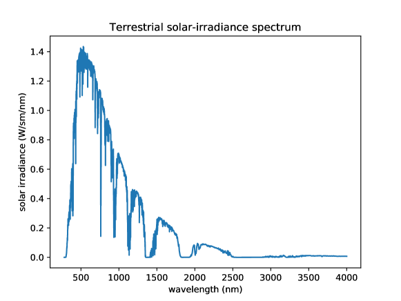
Figure 1.1. ASTM AM1.5 solar-irradiance spectrum [2], given by 2002 tabulated data points for wavelengths $\lambda$ from 280–4000nm. The spectrum is extremely oscillatory, with many sharp dips corresponding to absorption by various molecules.

Worse, for device design and optimization the integral (1.1) must be computed many times for different $f(\lambda)$ [1, 3, 4, 5, 6]. In these notes, we explain how eq. (1.1) can be accurately approximated with only a small number of $f(\lambda)$ evaluations by a Gaussian quadrature rule [7]

(1.2) $$\int_{a}^{b}S(\lambda)f(\lambda)d\lambda\approx\sum_{i=1}^{N}w_{i}f(\lambda_{i}),$$

where $\lambda_{i}$ are the quadrature points (nodes), $w_{i}$ are the quadrature weights, and $N$ is the order of the rule. The key fact is that we can construct a Gaussian quadrature rule in which the effect of the complicated irradiance function $S(\lambda)$ is precomputed in the $(w_{i},\lambda_{i})$ data, so that any polynomial $f(\lambda)$ of degree up to $2N-1$ is integrated exactly by eq. (1.2) and smooth $f(\lambda)$ are integrated with an error that decreases exponentially with $N$ [7, 8].

In the following notes, we first briefly review the numerical construction of Gaussian quadrature rules (Sec. 2), then present the resulting solar-weighted quadrature rules and demonstrate their accuracy on some examples (Sec. 3), and finally comment on various possible extensions and variations (Sec. 4). We provide a selection of precomputed rules (1.2) as well as a program in the Julia language [9] (in the form of a Jupyter notebook [10] tutorial) to compute a rule (1.2) for any desired $N$ and bandwidth $(a,b)$ [11].

2. Constructing Gaussian-quadrature rules

The construction of Gaussian quadrature rules, by which polynomial $f(\lambda)$ are integrated exactly up to a given degree, is closely tied to the theory of orthogonal polynomials [7]. For a given weight function $S(x)\geq 0$ and interval $(a,b)$, we define an inner product

(2.1) $$\langle p_{1},p_{2}\rangle=\int_{a}^{b}S(x)p_{1}(x)p_{2}(x)dx$$

of any polynomial functions $p_{1,2}(x)$. Then, by a Gram–Schmidt orthogonalization process applied to $\{1,x,x^{2},\ldots\}$, one can obtain a sequence of orthonormal polynomials $\{q_{0}(x),q_{1}(x),\ldots\}$ with respect to this inner product, where $q_{n}(x)$ has degree $n$. Remarkably, it turns out that the quadrature points $\lambda_{i}$ in eq. (1.2) are exactly the roots of $q_{N}(x)$, and the weights can also be computed from these polynomials [7].

Numerically, there are a variety of schemes for computing the quadrature points $\lambda_{i}$ and weights $w_{i}$. One of the simplest accurate methods is the Golub–Welsch algorithm [12], which constructs a tridiagonal “Jacobi” matrix corresponding to a three-term recurrence for the $q_{k}$ polynomials, and then obtains the nodes $\lambda_{i}$ and weights $w_{i}$ from the eigenvalues and eigenvectors of this matrix, respectively. It turns out that this procedure is equivalent to a Lanczos iteration for the symmetric linear operator corresponding to multiplication by $x$ [13]. The only input that is required is a way to compute the functional

(2.2) $$S\{p\}=\int_{a}^{b}S(x)p(x)dx,$$

which is just the integral (1.1) computed for any given polynomial $p(x)$ (up to degree $2N$). For the most famous applications of Gaussian quadrature to simple weight functions like $1$ on $(-1,1)$ (Gauss–Legendre quadrature), $e^{-x^{2}}$ on $(-\infty,+\infty)$ (Gauss–Hermite quadrature), or $e^{-x}$ on $(0,\infty)$ (Gauss–Laguerre quadrature), these integrals and the resulting three-term recurrences are known analytically. For an arbitrary weight function $S(x)$ like the solar-irradiance spectrum, we must perform integral (2.2) numerically (for $2N$ polynomials in total).

This process may at first seem fruitless: isn’t eq (2.2) equivalent to our original problem? There are two critical differences, however. First, polynomials $p(x)$ are very cheap to evaluate, so we can afford to use brute-force numerical integration methods that require $\sim 10^{4}$ function evaluations to evaluate (2.2), unlike solar-cell applications of eq. (1.1) where the integrand $f(\lambda)$ is very expensive. Second, we only need to perform these polynomial integrations once for a given $N$: we can then re-use the resulting quadrature rule $(\lambda_{i},w_{i})$ over and over for many different $f(\lambda)$.

In the specific case of our solar-irradiance spectrum $S(\lambda)$, the data are supplied in the form of 2002 data points from 280nm to 4000nm by the ASTM standard [2]. To define $S(\lambda)$ continuously for all $\lambda$ in this range, we perform a cubic-spline interpolation of the data using a library by Dierckx et al. [14]. More precisely, since we require an interpolant $S(\lambda)\geq 0$ everywhere in order for eq. (2.1) to define a proper inner product, we compute a cubic-spline interpolation $C(\lambda)$ of $\sqrt{S(\lambda)}$ at the ASTM data points, and then approximate $S(\lambda)$ by $C(\lambda)^{2}$ everywhere. This spline interpolant is shown for a portion of the spectrum from 400–500nm in Fig. 2.1.

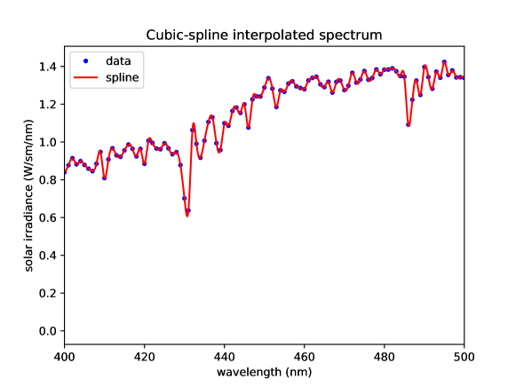
Figure 2.1. Cubic-spline interpolation [14] of the ASTM AM1.5 solar-irradiance spectrum [2], shown for a portion of the spectrum. To ensure positivity of the interpolant for all $\lambda$, we actually fit a spline $C(\lambda)$ to the square root of the irradiance, and approximate $S(\lambda)$ by $C(\lambda)^{2}$ for all $\lambda\in(280,4000)$nm.

A cubic spline has the property that not only does it pass through all of the data points, but its first and second derivatives are also continuous; the data points where the spline switches from one cubic curve to another (where the third derivative is discontinuous) are known as the knots of the spline [14]. In order to perform the $S\{p\}$ integrals (2.2) of polynomials $p(\lambda)$ against $C(\lambda)^{2}$, we simply break the integral into $\approx 2000$ segments at the knots (to avoid integrating through discontinuities) and apply a globally adaptive [15] Gauss–Kronrod [7] quadrature scheme implemented in Julia [16] to high accuracy ($>$ 9 digits).

Given an arbitrary weight function (and optionally a specialized routine to compute the $S\{p\}$ integrals), the QuadGK package in Julia [16] provides a subroutine to execute the Golub–Welsch algorithm and compute the quadrature points and weights. The only addition to the textbook description of the algorithm [13], besides the numerical computation of $S\{p\}$, is that the integration domain $(a,b)$ is internally rescaled to $(-1,1)$ so that the polynomials $p(x)$ can be represented in the basis of the Chebyshev polynomials $\{T_{0},T_{1},\ldots\}$ [17]. Given the coefficients $c_{k}$ of a Chebyshev series $p(x)=\sum_{j}a_{k}T_{k}(x)$, the polynomial $p(x)$ is evaluated by a Clenshaw recurrence [17], and another recurrence is used to compute the coefficients of the $xp(x)$ polynomial required for the Golub–Welsch algorithm [13]. This approach to representing and evaluating polynomials avoids the numerical problems (ill conditioning) that arise in the familiar monomial basis $\{1,x,x^{2},\ldots\}$—Chebyshev polynomials $T_{k}(x)=\cos(k\cos^{-1}x)$ are well-behaved numerically since they are “cosines in disguise” [17]. (A related, but more complicated, algorithm in which one first computes the “moments” $S\{T_{k}(x)\}$, is reviewed by Gautschi [19], and various other methods have also been proposed [19, 20, 21, 22].)

3. Solar integration rules and convergence

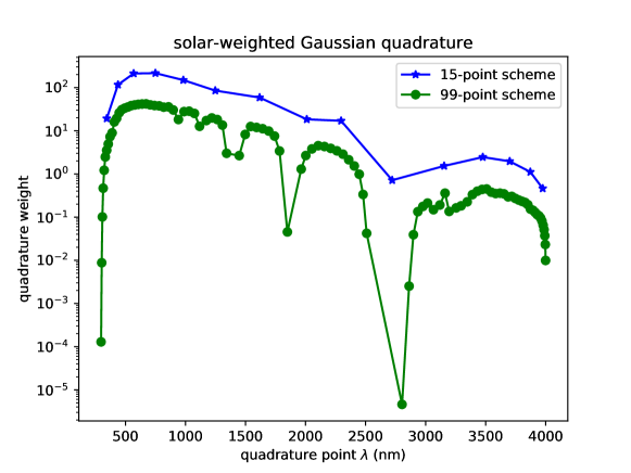
Figure 3.1. Solar-weighted Gaussian quadrature rules (ASTM AM1.5 spectrum [2]) in a bandwidth of 280–4000nm, for orders $N=15$ and $N=99$.

Given the computational methods in Sec. 2, we can then construct solar-weighted Gaussian quadrature rules for any desired order $N$ and any given bandwidth $\lambda\in(a,b)\subseteq(280,4000)\text{nm}$ using the code provided in the attached Julia notebook [11]. The resulting weights $w_{i}$ are plotted versus the corresponding quadrature points $\lambda_{i}$ for $N=15$ and $N=99$. Not surprisingly, they roughly follow the peaks and dips of the solar spectrum $S(\lambda)$ from Fig. 1.1.

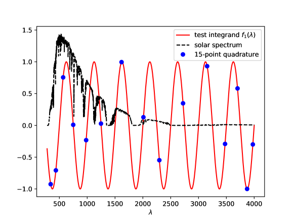
Figure 3.2. Test integrand $f_{1}(\lambda)=\sin(2\pi\lambda/500)$, superimposed on the solar-irradiance spectrum $S(\lambda)$. The blue dots show $f_{1}(\lambda_{i})$ at the quadrature points $\lambda_{i}$ of the $N=15$ point solar-weighted Gaussian quadrature rule from Fig. 3.1.

To validate these quadrature schemes and evaluate their accuracy, let us consider two test integrands, $f_{1}(\lambda)=\sin(2\pi\lambda/500)$ and $f_{2}(\lambda)=\sin(2\pi\lambda/50)$. The first integrand $f_{1}$ is shown in Fig. 3.2: it oscillates 8 times over the solar bandwidth, and seems to be barely sampled adequately by the $N=15$ point quadrature rule. To compute the “exact” integrals of $f_{1}$ and $f_{2}$, we apply the same method that we used for numerical polynomial integration $S\{p\}$ in Sec. 2: we partition the integral into $\approx 2000$ segments at the knots of the cubic-spline interpolant for $S(\lambda)$ and then apply an adaptive Gauss–Kronrod integration scheme to nearly machine precision ($>12$ significant digits). Comparing this brute-force result to that of the quadrature rules (1.2) applied to $f_{1}(\lambda)$ from Fig. 3.2, we find that the $N=15$ quadrature rule yields the correct result with an error of only $0.7\%$, while the $N=99$ quadrature rule yields the correct result to at least 13 significant digits.

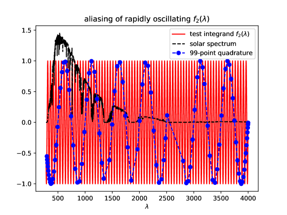
Figure 3.3. Test integrand $f_{2}(\lambda)=\sin(2\pi\lambda/50)$, superimposed on the solar-irradiance spectrum $S(\lambda)$. The blue dots show $f_{2}(\lambda_{i})$ at the quadrature points $\lambda_{i}$ of the $N=99$ point solar-weighted Gaussian quadrature rule from Fig. 3.1. This 99-point sampling is too coarse to capture the rapid oscillation of $f_{2}$, and results in an aliasing phenomenon [8] in which the sampled function appears to oscillate at a lower frequency.

For the test function $f_{2}(\lambda)$, which oscillates $10\times$ more rapidly than $f_{1}$, even the $N=99$ quadrature rule is not enough to obtain an accurate result: the sampling of $f_{2}$ is simply not fine enough to detect its rapid variations. This can be seen in Fig. 3.3, which depicts the function $f_{2}$ sampled at the quadrature points of the $N=99$ rule. The sampling clearly exhibits the phenomenon of aliasing, which is central to understanding the convergence rates of these quadrature schemes [8]: the sampled function $f_{2}(\lambda_{i})$ appears to oscillate at a much lower frequency. Since aliasing means that the quadrture rule cannot “perceive” the actual rapid oscillation of $f_{2}$, the quadrature formula (1.2) unsurprisingly yields a completely incorrect result ($>100$% error). A larger $N$ must be employed to integrate such a rapidly oscillating $f(\lambda)$. In the case of this $f_{2}(\lambda)$, an $N=140$ solar-weighted Gaussian quadrature rule is sufficient to compute $\int S(\lambda)f_{2}(\lambda)$ to 9 significant digits. The key point is that the required order of the quadrature rule is completely determined by the features of the application-supplied $f(\lambda)$, and is independent of the preprocessed complexity of the solar irradiance $S(\lambda)$.

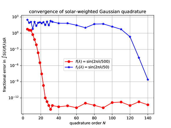
Figure 3.4. Convergence of solar-weighted Gaussian quadrature: fraction error in the integral $\int S(\lambda)f(\lambda)d\lambda$ versus the number $N$ of quadrature points for the two test integrands $f_{1}(\lambda)=\sin(2\pi\lambda/500)$ and $f_{2}(\lambda)=\sin(2\pi\lambda/50)$. In both cases, once $N$ becomes sufficiently large, the error falls exponentially with $N$. (However, in the case of the rapidly oscillating $f_{2}$ from Fig. 3.3, $N$ must first become $>100$ in order to adequately sample $f_{2}$’s oscillations.) The error in the $f_{1}$ does not drop below a “noise floor” of $\approx 10^{-13}$ due to the limitations of double-precision floating-point arithmetic [13].

In general, when Gaussian quadrature is applied to any smooth (infinitely differentiable) function $f(\lambda)$, such as an absorption spectrum, the error converges to zero faster than any power of $1/N$; typically (for analytic functions), the error converges exponentially with $N$ [8]. This rapid convergence is demonstrated in Fig. 3.4 for both $f_{1}$ and $f_{2}$. The accuracy of the $f_{1}$ integrand, in fact, nearly hits the limits of machine precision around $N\approx 30$ (and might be able to go slightly lower than $10^{-13}$ if we reduced the tolerances in the brute-force integration used in this section and in Sec. 2). The $f_{2}$ integration accuracy also exhibits exponential convergence, but the error does not begin its asymptotic decline until $N\gtrsim 100$, at which point the quadrature rule begins to adequately sample $f_{2}$’s rapid oscillation without destructive aliasing.

4. Extensions and variations

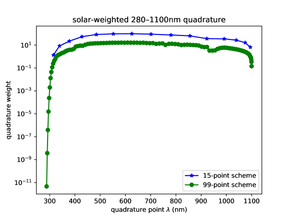
Figure 4.1. Solar-weighted Gaussian quadrature rules (ASTM AM1.5 spectrum [2]) in a bandwidth of 280–1100nm, for orders $N=15$ and $N=99$.

To apply the solar-weighted quadrature rule to specific applications, one may wish to consider some variations. For example, with silicon solar cells one rarely considers wavelengths beyond 1100nm, since longer wavelengths fall short of the bandgap of silicon and cannot easily generate electron–hole pairs [1, 4]. So, for these devices one might want a quadrature rule for $\int_{280\text{nm}}^{1100\text{nm}}S(\lambda)f(\lambda)d\lambda$. Two such quadrature rules, for $N=15$ and $N=99$ points, are shown in Fig. 4.1. It is advantageous to specialize the quadrature rule to the bandwidth of interest because one can then resolve much finer features in $f(\lambda)$ for the same number of points, and optimized solar cells typically exhibit many sharp resonant peaks [1, 3, 4]. As another example, the figure of merit for a photovoltaic cell is typically proportional to $\int S(\lambda)\lambda A(\lambda)d\lambda$ where $A(\lambda)$ is the device’s absorption spectrum [1], so one could also include the factor of $\lambda$ in the precomputed weight when constructing the Gaussian-quadrature schemes. It might also be useful to rescale the weight by the absorption coefficient of the photovoltaic material, to further skew the quadrature points towards the wavelengths where more absorption occurs.

Naturally, the same techniques could also be applied to completely different weight functions. Although weighted Gaussian quadrature schemes have been well known for decades in the numerical-integration literature, they seem to have been rarely applied for the complicated weighting functions that often arise in optical physics. For example, the CIE color-projection functions (used to model the perception of a human eye) [23] are described by tabulated data (though there are also analytical fits [24]), leading to integrals that qualitatively resemble Gauss–Hermite quadrature but require a quantitatively distinct quadrature scheme for high accuracy. Thermal emission from heated bodies is another good example: the emitted power is an integral of a surface’s absorption spectrum (found by solving Maxwell’s equations) weighted by a black-body “Planck” spectrum $\sim\omega^{3}/(e^{\hbar\omega/kT}-1)$ [25], suggesting a need for a Gauss–Laguerre-like Planck-weighted quadrature scheme.

References

- [1] P. Bermel, C. Luo, L. Zeng, L. C. Kimerling, and J. D. Joannopoulos, “Improving thin-film crystalline silicon solar cell efficiencies with photonic crystals,” Optics Express, vol. 15, no. 25, p. 16986, 2007.
- [2] ASTMG173-03, “Standard tables for reference solar spectral irradiances: Direct normal and hemispherical on 37 degree tilted surface,” ASTM International, West Conshohocken, PA, Tech. Rep., 2005.
- [3] X. Sheng, S. G. Johnson, J. Michel, and L. C. Kimerling, “Optimization-based design of surface textures for thin-film Si solar cells,” Optics Express, vol. 19, pp. A841–A850, June 2011.
- [4] A. Oskooi, P. A. Favuzzi, Y. Tanaka, H. Shigeta, Y. Kawakami, and S. Noda, “Partially disordered photonic-crystal thin films for enhanced and robust photovoltaics,” Applied Physics Letters, vol. 100, no. 18, p. 181110, 2012.
- [5] C. Lin, L. J. Martínez, and M. L. Povinelli, “Experimental broadband absorption enhancement in silicon nanohole structures with optimized complex unit cells,” Optics Express, vol. 21, no. S5, p. A872, 2013.
- [6] S. Wiesendanger, M. Zilk, T. Pertsch, F. Lederer, and C. Rockstuhl, “A path to implement optimized randomly textured surfaces for solar cells,” Applied Physics Letters, vol. 103, no. 13, p. 131115, 2013.
- [7] H. Brass and K. Petras, Quadrature Theory: The Theory of Numerical Integration on a Compact Interval, ser. Mathematical Surveys and Monographs. Providence, RI: American Mathematical Society, 2011, vol. 178.
- [8] L. N. Trefethen, “Is Gauss quadrature better than Clenshaw–Curtis?” SIAM Review, vol. 50, no. 1, pp. 67–87, 2008.
- [9] J. Bezanson, A. Edelman, S. Karpinski, and V. B. Shah, “Julia: A fresh approach to numerical computing,” SIAM review, vol. 59, no. 1, pp. 65–98, 2017.
- [10] T. Kluyver, B. Ragan-Kelley, F. Pérez, B. Granger, M. Bussonnier, J. Frederic, K. Kelley, J. Hamrick, J. Grout, S. Corlay, P. Ivanov, D. Avila, S. Abdalla, and C. Willing, “Jupyter notebooks—a publishing format for reproducible computational workflows,” in Positioning and Power in Academic Publishing: Players, Agents and Agendas, F. Loizides and B. Schmidt, Eds. IOS Press, 2016, pp. 87–90.
- [11] S. G. Johnson, “Solar-weighted Gaussian quadrature,” https://nbviewer.jupyter.org/urls/math.mit.edu/~stevenj/Solar-Quadrature.ipynb, accessed: 2019-12-13.
- [12] G. H. Golub and J. H. Welsch, “Calculation of Gauss quadrature rules,” Mathematics of Computation, vol. 23, no. 106, pp. 221–221, 1969.
- [13] L. N. Trefethen and D. Bau, Numerical Linear Algebra. SIAM, 1997.
- [14] P. Dierckx, Curve and Surface Fitting with Splines. Oxford University Press, 1993.
- [15] M. A. Malcolm and R. B. Simpson, “Local versus global strategies for adaptive quadrature,” ACM Transactions on Mathematical Software, vol. 1, no. 2, pp. 129–146, 1975.
- [16] S. G. Johnson, “QuadGK.jl: Gauss–Kronrod integration in Julia,” https://github.com/JuliaMath/QuadGK.jl, accessed: 2019-12-13.
- [17] L. N. Trefethen, Approximation Theory and Approximation Practice. SIAM, 2012.
- [18] S. Olver and A. Townsend, “A practical framework for infinite-dimensional linear algebra,” in Proceedings of the 1st Workshop for High Performance Technical Computing in Dynamic Languages – HPTCDL ‘14. IEEE, 2014.
- [19] W. Gautschi, “Algorithm 726: ORTHPOL—a package of routines for generating orthogonal polynomials and Gauss-type quadrature rules,” ACM Transactions on Mathematical Software, vol. 20, no. 1, pp. 21–62, 1994.
- [20] G. Mantica, “A stable Stieltjes technique for computing orthogonal polynomials and jacobi matrices associated with a class of singular measures,” Constructive Approximation, vol. 12, no. 4, pp. 509–530, 1996.
- [21] M. J. Gander and A. H. Karp, “Stable computation of high order Gauss quadrature rules using discretization for measures in radiation transfer,” Journal of Quantitative Spectroscopy and Radiative Transfer, vol. 68, no. 2, pp. 213–223, 2001.
- [22] A. D. Fernandes and W. R. Atchley, “Gaussian quadrature formulae for arbitrary positive measures,” Evolutionary Bioinformatics Online, vol. 2, pp. 251–259, Jan. 2006.
- [23] J. Schanda, Colorimetry: Understanding the CIE System. New York, NY: Wiley, 2007.
- [24] C. Wyman, P.-P. Sloan, and P. Shirley, “Simple analytic approximations to the CIE XYZ color matching functions,” Journal of Computer Graphics Techniques (JCGT), vol. 2, no. 2, pp. 1–11, July 2013.
- [25] C. M. Cornelius and J. P. Dowling, “Modification of Planck blackbody radiation by photonic band-gap structures,” Physical Review A, vol. 59, no. 6, pp. 4736–4746, 1999.