Fourth-order moment of the light field in atmosphere

Abstract

The quasiclassical distribution function for photon density in the phase space is obtained from solution of the kinetic equation. This equation describes propagation of paraxial laser beams in the Earth atmosphere where “collision integral” embodies the influence of turbulence. The anisotropy of photon distribution is shown and explained. For long propagation path, the explicit expression for fourth-order moment of light is obtained as a sum of linear and quadratic forms of the average distribution function. This moment describes a spatial correlation of four light waves, giving the information about the photon distribution in the cross-section of the beam. The fourth moment can be measured using two small detectors outside the central part of the beam. The linear form describes the shot noise (quantum fluctuations) of photons. The range where the shot noise exceeds the classical noise is found analytically. Derived photon fluctuations are the valuable source of information about statistical properties and local structure of the laser radiation that can be used for applications.

I Introduction

Propagation of laser beam in atmosphere is crucial part for current developments of classic and quantum communication and remote sensing systems. Among others description of influence of turbulence is important for such areas as quantum key distribution veloresi ; usenko , satellite-ground communication Hosseinidehaj ; Aspelmeyer , quantum teleportation ma ; ren ; Hofmann , propagation of entangled and squeezed states ursin ; yin ; Peuntinger ; vasylev2016 , and ghost imaging wang ; Shi . In all these cases changes of spatio-temporal properties of initial radiation due to presence of atmospheric turbulence plays vital role.

Laser beam characteristics can be significantly modified in the course of light propagation in atmosphere. Atmospheric eddies generate random fluctuations in the air refractive index (RI) which cause an additional beam broadening as well as a wandering effect Tatarskii1 ; Fante1 ; Fante2 ; Kravtsov ; Gorshkov . The results of individual beam-eddy collisions depend on their characteristic dimensions. In the case of prevailing small-size eddies, the beam broadening is observed. In contrast, for the case of small beam radius, the light can be deflected as a whole showing the effect of wandering. Despite the very small fluctuations in RI, their impact on the beam evolution can be quite significant because of accumulating effect which occurs along the propagation path. Wide dispersion of eddies parameters and index-of-refraction structure constants $C^{2}_{n}$ complicate the possibility of numerical research for these systems.

A spatio-temporal distribution of the radiation intensity can be obtained using different approaches. The situation is much more intricate for the description of fluctuations of light intensity. The fluctuations are described by four-wave correlation functions (fourth-order moments of optical field) of propagating radiation. In the course of propagation, the initially coherent laser radiation acquires some properties of Gaussian statistics DeWolf because of the effect of atmospheric turbulence. This complicates a theoretical analysis of fluctuation characteristics.

In early studies, the equations governing evolution of fourth-order moments were proposed Fante1 ; Fante2 . However, usefulness of these equations is questionable because of their complexity. Later on, the alternative approach, based on the photon distribution function (PDF) and the kinetic equation for it, was used berm ; berm2009 ; baskov2016 . This function was defined as the photon density in the phase space. For long-distance propagation the effect of atmospheric eddies is described via random force in the kinetic equation. Obviously, this classical force cannot adequately consider the collisions which are accompanied by a substantial change of the photon momentum. In the paper baskov2018 a more general approach which overcomes this restriction was proposed. The theory was modified, providing more general first-principle approach in order to account for the effect of photon-eddy interactions by means of collision integral. Moreover, a random nature of photon-eddy collisions is accounted for by the Langevin source with known statistical properties Kogan ; Tom . As a result, a linear Boltzmann-Langevin equation describes both the average and fluctuating parts of photon distribution.

The goal of this paper is to derive asymptotical value for the fourth moment. It is highly demanded in bunch of applied researches such as intensity correlation Vellekoop ; Newman , enhanced focusing Popoff ; Vellekoop2 , different imaging problems Katz ; Hardy ; Zhang_imag . The fourth moment problem is simplified if the light beam is affected by multiple collisions with turbulent eddies leading to the Gaussian (normal) statistics of radiation. In this case the fourth moments can be expressed in terms of the average distribution function.

The remainder of this paper is organized as follows. In Sec. II, we obtain the fourth-order moment expressed in terms of average distribution function. In Sec. III, the kinetic equations for the average distribution function and its fluctuations are briefly analyzed. Section IV contains technical details of analytical solution for the PDF and may be skipped by the uninterested reader. The explicit form for PDF is used for obtaining the fourth-moment asymptotics in Sec. V. The derived fourth moment is applied to estimation of aperture-averaged scintillations. The results of calculations are analyzed in Sec. VI. In Appendix B, the asymptotics of distribution functions, which are solutions of two different kinetic equations, are compared.

II Distribution function of photons and long-distance fourth-order moment for field.

The photon distribution function, defined by analogy with distribution functions in physics of solids is given by UJP

$$\hat{f}({\bf r},{\bf q},t)=\frac{1}{V}\sum_{\bf k}e^{-i{\bf k\cdot r}}b^{\dagger}_{{\bf q}+{\bf k}/2}b_{{\bf q}-{\bf k}/2},$$ (1)

where $b^{\dagger}_{\bf q}$ and $b_{\bf q}$ are quantum amplitudes of bosonic photon field with the wave vector ${\bf q}$; $V\equiv L_{x}L_{y}L_{z}\equiv SL_{z}$ is the normalizing volume. The system should be large enough to prevent the effect of boundary conditions on beam propagation. All operators are given in the Heisenberg representation. The laser beam propagates in the $z$ direction. Only small divergence of the beam components is assumed, i.e. the paraxial approximation holds. In this case, the initial polarization of light remains almost unaffected for a wide range of propagation distances (see Ref. stroh ).

The operator $\hat{f}({\bf r},{\bf q},t)$, describing the photon density in the $({\bf r},{\bf q})$ space, after summing over all values of $\bf q$ gives the density of photons only in the spatial domain

$$\hat{I}({\bf r},t)=\frac{1}{V}\sum_{\bf q,k}e^{-i{\bf k\cdot r}}b^{\dagger}_{{\bf q}+{\bf k}/2}b_{{\bf q}-{\bf k}/2}.$$ (2)

The characteristic sizes of spatial inhomogeneities described by both operators, $\hat{f}({\bf r},{\bf q},t)$ and $\hat{I}({\bf r},t)$, are assumed much greater than the optical wavelength $\lambda=(2\pi/q_{0})$. Here $q_{0}$ is the wave vector corresponding to the central frequency of the radiation, $\omega_{0}=cq_{0}$. Therefore it is quite reasonable to restrict the sums in Eqs. (1) and (2) by the range of small $k$, i.e. $k<k_{0}$ such that the inequality $k_{0}\ll q_{0}$ is satisfied. At the same time, the value of $k_{0}$ must be large enough to provide the desired spatial accuracy of the beam description. If the characteristic size of the radiation inhomogeneity is $\delta r$, then the inequality $k_{0}\delta r\gg 1$ must be satisfied. Taking into account that the uncertainty of ${\bf q}$ ($\delta q$) is given by $(k/2)\leq k_{0}/2$, we conclude that $\delta q\delta r\gg 1/2$, satisfying the Heisenberg inequality. The above considerations explain what types of optical properties can be studied using the distribution function. A similar idea of coarse-grained description of light has been used before (see, for example, the monograph by Mandel and Wolf Mandel and Kolobov’s review Kolobov ).

The operator of photon density can be represented as

$$\hat{I}({\bf r},t)=\langle\hat{I}({\bf r},t)\rangle+\delta\hat{I}({\bf r},t),$$ (3)

where $\langle\hat{I}({\bf r},t)\rangle$ and $\delta\hat{I}({\bf r},t)$ are the average and fluctuating constituents of $\hat{I}({\bf r},t)$. The averaging includes the quantum-mechanical averaging of operators $\hat{f}$ and $\hat{I}$ and averaging over many ”runs” of the beam through different realizations of turbulence relief. Both averaging are performed independently.

Average product of photon densities is defined by

$$\langle\hat{I}({\bf r},t)\hat{I}({\bf r^{\prime}},t)\rangle{=}\hskip 142.26378pt$$ (4)

$$\frac{1}{V^{2}}\sum_{\begin{subarray}{c}{\bf q,k}\\ {\bf q^{\prime},k^{\prime}}\end{subarray}}e^{-i({\bf k}\cdot{\bf r}{+}{\bf k^{\prime}}\cdot{\bf r^{\prime}})}\langle b^{\dagger}_{{\bf q}{+}\frac{\bf k}{2}}b_{{\bf q}{-}\frac{\bf k}{2}}b^{\dagger}_{{\bf q^{\prime}}{+}\frac{\bf k^{\prime}}{2}}b_{{\bf q^{\prime}}{-}\frac{\bf k^{\prime}}{2}}\rangle.$$

All operators on the right side are given at time $t$ which is a propagation time. It is reasonable to consider that the average product of four operators at asymptotically large $t$ splits into products of pairs, i.e.,

$$\langle b^{\dagger}_{{\bf q}{+}\frac{\bf k}{2}}b_{{\bf q}{-}\frac{\bf k}{2}}b^{\dagger}_{{\bf q^{\prime}}{+}\frac{\bf k^{\prime}}{2}}b_{{\bf q^{\prime}}{-}\frac{\bf k^{\prime}}{2}}\rangle{\approx}\langle b_{{\bf q}{+}\frac{\bf k}{2}}^{\dagger}b_{{\bf q}{-}\frac{\bf k}{2}}\rangle\langle b_{{\bf q}^{\prime}{+}\frac{{\bf k}^{\prime}}{2}}^{\dagger}b_{{\bf q}^{\prime}{-}\frac{{\bf k}^{\prime}}{2}}\rangle\hskip 14.22636pt$$ (5)

$${+}\langle b_{{\bf q}+\frac{\bf k}{2}}^{\dagger}b_{{\bf q}^{\prime}-\frac{{\bf k}^{\prime}}{2}}\rangle\langle b_{{\bf q}^{\prime}+\frac{{\bf k}^{\prime}}{2}}^{\dagger}b_{{\bf q}{-}\frac{\bf k}{2}}\rangle{+}\langle b_{{\bf q}{+}\frac{\bf k}{2}}^{\dagger}b_{{\bf q^{\prime}}{-}\frac{\bf k^{\prime}}{2}}\rangle\delta_{{\bf q}{-}\frac{\bf k}{2},{\bf q^{\prime}}{+}\frac{\bf k^{\prime}}{2}}.$$

In other words, it is assumed that amplitudes $b^{\dagger}$ and $b$ obey Gaussian statistics. Such assumption is justified since for $t\rightarrow\infty$ each primary coherent electromagnetic wave experiences multiple scatterings by randomly distributed vortices Das ; DeWolf . The ”collisions” randomize photon momenta. (This is in contrast to the paper Zhang in which the Gaussian statistics was assumed from the very beginning of photon trajectory.) It is also considered that the condition of paraxial approximation is still fulfilled, and therefore the wave vector component $q_{z}$ remains almost unchanged (approximately equal to $q_{0}$). This means that the RI variation in the $z$-direction has no significant effect on propagation of paraxial beams Tatarskii1 . This phenomenon is interpreted in baskov2018 as arising from relativistic length contraction of moving objects (the relative motion of vortices and photons). The perpendicular constituent ${\bf q}_{\bot}$, where ${\bf q}_{\bot}=\{q_{x},q_{y}\}$, grows with time like Brownian particles moving in the ${\bf q}_{\bot}$-space (see berm ).

Substituting (5) into (4), we obtain

$$\langle\hat{I}({\bf r},t)\hat{I}({\bf r^{\prime}},t)\rangle{\approx}\frac{1}{V^{2}}\sum_{\begin{subarray}{c}{\bf q,k}\\ {\bf q^{\prime},k^{\prime}}\end{subarray}}e^{-i({\bf k}\cdot{\bf r}{+}{\bf k^{\prime}}\cdot{\bf r^{\prime}})}\times\hskip 71.13188pt$$ (6)

$$\left[\langle b_{{\bf q}+\frac{\bf k}{2}}^{\dagger}b_{{\bf q}-\frac{\bf k}{2}}\rangle\langle b_{{\bf q}^{\prime}+\frac{{\bf k}^{\prime}}{2}}^{\dagger}b_{{\bf q}^{\prime}-\frac{{\bf k}^{\prime}}{2}}\rangle\right.{+}\langle b_{{\bf q}+\frac{\bf k}{2}}^{\dagger}b_{{\bf q}^{\prime}-\frac{{\bf k}^{\prime}}{2}}\rangle\langle b_{{\bf q}^{\prime}+\frac{{\bf k}^{\prime}}{2}}^{\dagger}b_{{\bf q}-\frac{\bf k}{2}}\rangle$$

$${+}\left.\langle b_{{\bf q}+\frac{\bf k}{2}}^{\dagger}b_{{\bf q^{\prime}}-\frac{\bf k^{\prime}}{2}}\rangle\delta_{{\bf q}-\frac{\bf k}{2},{\bf q^{\prime}}+\frac{\bf k^{\prime}}{2}}\right].\hskip 14.22636pt$$

Utilizing here the definitions (1) and (2), we arrive at more meaningful form

$$\langle\hat{I}({\bf r},t)\hat{I}({\bf r^{\prime}},t)\rangle=\delta({\bf r}-{\bf r^{\prime}})\langle\hat{I}({\bf r},t)\rangle+\langle\hat{I}({\bf r},t)\rangle\langle\hat{I}({\bf r^{\prime}},t)\rangle\hskip 14.22636pt$$ (7)

$$+\sum_{{\bf q},{\bf q^{\prime}}}\langle f(\frac{{\bf r}+{\bf r^{\prime}}}{2},{\bf q})\rangle\langle f(\frac{{\bf r}+{\bf r^{\prime}}}{2},{\bf q^{\prime}})\rangle e^{i({\bf q^{\prime}}-{\bf q})\cdot({\bf r}-{\bf r^{\prime}})}.$$

The third term in the right side is obtained by formal changing the indices in the operators $b_{\bf q}$, $b_{\bf q}^{\dagger}$, and exponential multiplier as follows

$${\bf k}\rightarrow{\bf q}-{\bf q^{\prime}}+\frac{{\bf k}+{\bf k^{\prime}}}{2},\quad{\bf k^{\prime}}\rightarrow{\bf q^{\prime}}-{\bf q}+\frac{{\bf k}+{\bf k^{\prime}}}{2}$$

$${\bf q}\rightarrow\frac{1}{2}\left({\bf q}+{\bf q^{\prime}}+\frac{{\bf k}-{\bf k^{\prime}}}{2}\right),\quad{\bf q^{\prime}}\rightarrow\frac{1}{2}\left({\bf q}+{\bf q^{\prime}}-\frac{{\bf k}-{\bf k^{\prime}}}{2}\right).$$

It can be written in a simpler form

$$\bigg{|}\sum_{\bf q}\langle f\left(\frac{{\bf r}+{\bf r^{\prime}}}{2},{\bf q}\right)\rangle e^{i{\bf q}\cdot({\bf r^{\prime}}-{\bf r})}\bigg{|}^{2}\equiv\bigg{|}\mathscr{F}\left(\frac{{\bf r}+{\bf r^{\prime}}}{2},{\bf r}-{\bf r^{\prime}}\right)\bigg{|}^{2},$$

where

$$\mathscr{F}({\bf r}_{1},{\bf r}_{2})=\sum_{\bf q}\langle\hat{f}({\bf r}_{1},{\bf q})\rangle\exp(-i{\bf q}\cdot{\bf r}_{2})$$

is the Fourier transform of $\langle\hat{f}({\bf r}_{1},{\bf q})\rangle$ in q domain.

The equation (7) represents the result of mixing four light waves after propagation of the beam over long distances in the $z$ direction. The first term in the right side describes the shot noise. It has a quantum nature and is important in the case of low photon density. The second term is the product of average photon densities. It does not consider the correlation of light intensity at different positions ${\bf r}$ and ${\bf r^{\prime}}$ and is not present in the average product of fluctuations $\langle\delta\hat{I}({\bf r},t)\delta\hat{I}({\bf r^{\prime}},t)\rangle$. The third term, like the first one, describes fluctuations. It is given by a quadratic form of PDF which in general case does not reduce to the product of photon densities $\langle\hat{I}({\bf r},t\rangle$.

The point ${\bf r}={\bf r}^{\prime}$ is the exception where the second and third terms become equal to each other. As a result, the scintillation index, $\sigma^{2}$, defined by

$$\sigma^{2}=\frac{{\langle\hat{I}^{2}}\rangle-{\langle\hat{I}\rangle^{2}}}{{\langle\hat{I}\rangle^{2}}},$$ (8)

is equal to unity regardless of $\bf{r}$. [We neglect the shot noise here.] This is the well-known result for saturated regime of scintillation DeWolf . It should be emphasized that this result is obtained only from the conditions of the Gaussian statistics for field operators in PDF.

The individual terms in Eq. (7)

$$\langle f(\frac{{\bf r}+{\bf r^{\prime}}}{2},{\bf q})\rangle\langle f(\frac{{\bf r}+{\bf r^{\prime}}}{2},{\bf q^{\prime}})\rangle e^{i({\bf q^{\prime}}-{\bf q})\cdot({\bf r}-{\bf r^{\prime}})},$$ (9)

contribute to the correlation function of photon densities in different points ${\bf r}$ and ${\bf r^{\prime}}$. At the same time, both photon distribution functions in (9) depend on the same spatial coordinate ${({\bf r}+{\bf r^{\prime}})}/{2}$ which is different from ${\bf r}$ and ${\bf r^{\prime}}$. As a result the correlation of photon densities at different positions ${\bf r}$ and ${\bf r^{\prime}}$ depends on the values of PDF at $({\bf r}+{\bf r^{\prime}})/2$. In particular, this may be the beam center (if ${\bf r}=-{\bf r^{\prime}}$) where the PDF can have the maximum value. The discussed example indicates that by studying the photon fluctuations outside the center of the beam, we can get information about its central region.

The physical nature of the third term is similar to the Hanbury Brown-Twiss effect Zubairy which describes four-wave correlations. The properties of the radiation field which are due to the spatial correlation of the irradiation density can be used in practice Garnier .

Explicit value for the third term is very simple in ”coordinate representation” (widely used in theory of photoelectric measurements, see Mandel ) which is based on modified light amplitudes. The latter are given by

$$b_{\bf r}=(b^{\dagger}_{\bf r})^{\dagger}=\frac{1}{\sqrt{V}}\sum_{\bf q}e^{i{\bf qr}}b_{\bf q}.$$

Using these variables, the third term is expressed as $|\langle b^{{\dagger}}_{\bf r}b_{\bf r^{\prime}}\rangle|^{2}$. To obtain such a simple formula, the definition of PDF was used.

It is reasonable to consider that for large values of difference $|{\bf r}-{\bf r}^{\prime}|$, there is no correlation between amplitudes $b_{\bf r}^{\dagger}$ and $b_{{\bf r}^{\prime}}$. Conversely, non-zero value of $|\langle b^{{\dagger}}_{\bf r}b_{\bf r^{\prime}}\rangle|^{2}$ indicates the presence of correlation of photon density at the points ${\bf r}$ and ${\bf r^{\prime}}$. Using two detectors at these points, we can directly obtain the correlation function of fluctuations and compare it with the theoretical value $|\langle b^{{\dagger}}_{\bf r}b_{\bf r^{\prime}}\rangle|^{2}$.

Equation (8) represents a relative fluctuation of photon density at the specified locations where ${\bf r}={\bf r}^{\prime}$. It is reasonable to expect that the total photon flux in the $z$-direction defined by

$$I_{T}(z,t)=c\int d{\bf r}_{\bot}\hat{I}({\bf r})$$ (10)

does not fluctuate due to the lack of absorption. The following considerations elucidate this point. A size of fluctuations of $I_{T}(z,t)$ can be described by the average $\langle[\delta I_{T}(z,t)]^{2}\rangle$. Integration in the $(x,y)$ plane results in

$$\langle[\delta I_{T}(z,t)]^{2}\rangle=c^{2}S\sum_{{\bf q}_{\bot}}\int d{\bf r}_{\bot}\langle\hat{f}({\bf r},{\bf q})\rangle^{2}.$$ (11)

Equation (11) is obtained using the relationships

$$\int d({\bf r}_{\bot}{-}{\bf r}_{\bot}^{\prime})e^{i({\bf q}_{\bot}-{\bf q}_{\bot}^{\prime})\cdot({\bf r}_{\bot}-{\bf r}_{\bot}^{\prime})}=(2\pi)^{2}\delta({\bf q}_{\bot}{-}{\bf q}_{\bot}^{\prime})$$

and

$$\delta({\bf q}_{\bot}{-}{\bf q}_{\bot}^{\prime})=\frac{S}{(2\pi)^{2}}\delta_{{\bf q}_{\bot},{\bf q}_{\bot}^{\prime}}.$$

The estimate for the relative fluctuations, which uses Eq.(8), is given by

$$\frac{\langle[\delta I_{T}(z,t)]^{2}\rangle}{{\langle I_{T}(z,t)\rangle}^{2}}\propto({\bar{q}}_{\bot}R)^{-2},$$ (12)

where symbols ${\bar{q}}_{\bot}$ and $R$ denote characteristic momentum of $q_{\bot}$ and the beam radius, respectively. Both of these quantities increase with time $t$. Therefore the right side of Eq. (12) asymptotically goes to zero. This is a typical situation for many-particle systems: usually relative fluctuations of total numbers of particles are negligible. The same applies to multiphoton system in this work.

Behavior of physical quantities ${\bar{q}}_{\bot}$ and $R$ was investigated in earlier papers (see, for example, berm ) using the approach of “slowly varying force”. In what follows, our consideration is based on the alternative collision-integral method.

III Boltzmann-Langevin equation for photon distribution function.

Kinetic equation governing the evolution of photon density in the phase space, $\hat{f}({\bf r},{\bf q},t)$, can be represented by baskov2018

$$\partial_{t}\hat{f}({\bf r},{\bf{q}},t)+{\bf c_{q}}\cdot\partial_{\bf r}\hat{f}({\bf r},{\bf q},t)=\hat{K}({\bf r},{\bf q},t)-\hat{\nu}_{\bf q}\big{\{}\hat{f}({\bf r},{\bf q},t)\},$$ (13)

where ${\bf c_{q}}={\partial\omega_{q}}/{\partial\bf q}=c{\bf q}/q_{0}$. Random nature of individual collisions is taken into account by the Langevin source of fluctuations, $\hat{K}({\bf r},{\bf q},t)$. The Langevin approach is widely used in quantum optics Zubairy and physics of solids Kogan . This approach uses stochastic differential equation for modeling the dynamics of physical systems (see BHARUCH ). The “collision” integral $\hat{\nu}_{\bf q}$ is given by

$$\hat{\nu}_{\bf q}\big{\{}\hat{f}({\bf r},{\bf q},t)\}=\frac{2\pi\omega_{0}^{2}}{c} \int d{\bf k^{\prime}_{\bot}}\psi({\bf k^{\prime}_{\bot}})$$

$$\times \big{(}\hat{f}({\bf r},{\bf q},t)-\hat{f}({\bf r},{\bf q+k^{\prime}_{\bot}},t)\big{)},$$

where $\psi({\bf k^{\prime}_{\bot}})=\frac{V}{(2\pi)^{3}}\langle|n_{\bf k^{\prime}_{\bot}}|^{2}\rangle$ and $n_{\bf k}$ is the Fourier transform of the fluctuating refraction index $\delta n({\bf r})$:

$$n_{\bf k}=\frac{1}{V}\int dVe^{i{\bf k\cdot r}}\delta n({\bf r}).$$ (15)

The von Karman formula

$$\psi({\bf k})=0.033C_{n}^{2}\frac{\exp(-(kl_{0}^{\prime})^{2})}{(k^{2}+L_{0}^{-2})^{11/6}},$$ (16)

provides a reliable description of atmospheric turbulence by means of the set of parameters $C_{n}^{2}$, $l_{0}^{\prime}$ and $L_{0}$. These parameters take into account the turbulence strength and the vortex shape.

Linear inhomogeneous equation (13) can be used for the description of both the evolution of photon distribution and photon fluctuations. The term $\hat{\nu}_{\bf q}\big{\{}\hat{f}({\bf r},{\bf q},t)\}$ describes photon-eddies scattering. It follows from Eq. (III) that the quantity

$$W({\bf k^{\prime}_{\bot}})=\frac{(2\pi)^{3}\omega_{0}^{2}}{Sc}\psi({\bf k^{\prime}_{\bot}})$$

can be interpreted as the probability per unit time of a photon transition from state ${\bf q}_{\bot}$ to state ${\bf q}_{\bot}\pm{\bf k}^{\prime}_{\bot}$. In what follows, we will use the quantity

$$\nu=\frac{2\pi\omega_{0}^{2}}{c}\int d{\bf k^{\prime}_{\bot}}\psi({\bf k^{\prime}_{\bot}})$$ (17)

as a convenient parameter which describes the relaxation in the system and does not depend on photon variables.

After averaging of Eq. (13), the Langevin source disappears and the kinetic equation for $\langle\hat{f}({\bf r},{\bf q},t)\rangle$ reduces to

$$[\partial_{t}+{\bf c_{q}}\cdot\partial_{\bf r}+\hat{\nu}_{\bf q}]\langle\hat{f}({\bf r},{\bf{q}},t)\rangle=0.$$ (18)

The kinetic equation for the fluctuating component

$$\delta f({\bf r},{\bf{q}},t)=\hat{f}({\bf r},{\bf{q}},t)-\langle\hat{f}({\bf r},{\bf{q}},t)\rangle$$ (19)

is given by

$$[\partial_{t}+{\bf c_{q}}\cdot\partial_{\bf r}+\hat{\nu}_{\bf q}]\delta f({\bf r},{\bf{q}},t)=\hat{K}({\bf r},{\bf q},t).$$ (20)

Two linear equations (18) and (20) can be used for obtaining average and fluctuating PDF. The state of a radiation field in the source aperture determines the boundary conditions for $\langle\hat{f}\rangle$. The free term, $K$, distributed along the beam path, is the only source of non-trivial solution of (20) if photon fluctuations in the outgoing aperture are neglected.

IV Analytical solution for average PDF.

The homogeneous equation (18) can be solved using the Fourier transforms. To do this, we multiply all terms in $(\ref{18my})$ by $\frac{1}{S}\times e^{i{\bf k_{\bot}}\cdot{\bf r}}$ and integrate over ${\bf r_{\bot}}$. [In what follows, we use the notation $f({\bf r},{\bf q},t)$ for $\langle\hat{f}({\bf r},{\bf q},t)\rangle$.] As a result, we obtain for the Fourier component, defined by

$$f({\bf k_{\bot}},{\bf q},t)=\frac{1}{S}\int d{\bf r_{\bot}}f({\bf r},{\bf{q}},t)e^{i{\bf k_{\bot}}\cdot{\bf r}},$$ (21)

a simpler equation

$$(\partial_{t}-i{\bf k}_{\bot}\cdot{\bf c}_{{\bf q}_{\bot}})f({\bf k_{\bot}},{\bf q_{\bot}},t)=-\hat{\nu}_{\bf q_{\bot}}\big{\{}f({\bf k}_{\bot},{\bf q}_{\bot},t)\},$$ (22)

in which ${\bf c}_{{\bf q}_{\bot}}=c{{\bf q}_{\bot}}/{q_{0}}$ and $|{\bf c}_{{\bf q}_{\bot}}|\ll c$. In the course of derivation of Eq. (22) we consider $z=ct$ (see Appendix A). Since the $z$ components of vectors are not in the last equations, we omit the notation $\bot$ for the brevity of the body text (except Appendix B) and consider only $x$- and $y$-components. Solution of equation (22) can be represented as the product

$$f({\bf k},{\bf q},t)=e^{i{\bf k}\cdot{\bf q}\frac{ct}{q_{0}}}\times\varphi({\bf k},{\bf q},t),$$

where the new function $\varphi$ satisfies the integral equation

$$\partial_{t}\varphi({\bf k},{\bf q},t){=}{-}\frac{2\pi\omega_{0}^{2}}{c}{\int}d{\bf k^{\prime}}\psi({\bf k^{\prime}})\times\hskip 99.58464pt$$ (23)

$$\bigg{[}\varphi({\bf k},{\bf q},t)-e^{i{\bf k}\cdot{\bf k^{\prime}}\frac{ct}{q_{0}}}\varphi({\bf k},{\bf q}{+}{\bf k^{\prime}},t)\bigg{]}.$$

Another Fourier transform,

$$\Phi({\bf k},{\bf p},t)=S^{-1}\sum_{\bf q}e^{{-i\bf p}\cdot{\bf q}}\varphi({\bf k},{\bf q},t),$$ (24)

reduces the kinetic equation to the relaxation type equation

$$\partial_{t}\Phi({\bf k},{\bf p},t)=-\gamma({\bf k},{\bf p},t)\Phi({\bf k},{\bf p},t).$$ (25)

The relaxation frequency $\gamma$ is given by

$$\gamma({\bf k},{\bf p},t)=\frac{4\pi\omega_{0}^{2}}{c}\int d{\bf k^{\prime}_{\bot}}\psi({\bf k^{\prime}_{\bot}})\sin^{2}\bigg{[}\bigg{(}{\bf p}-{\bf k}\frac{ct}{q_{0}}\bigg{)}{\cdot}\frac{\bf k^{\prime}_{\bot}}{2}\bigg{]}.$$ (26)

The set of independent variables ${{\bf p},\bf k},t$, forms the vector ${\bf P}(t)={\bf p}-{\bf k}tc/q_{0}$, on which the relaxation parameter depends: $\gamma\equiv\gamma\big{(}{\bf P}(t)\big{)}$. In the case of large characteristic values of ${\bf P}(t)\cdot{\bf k}^{\prime}/2$, the quantity of $\gamma$ approaches $\nu$ [see Eq. (17)].

Solution of Eq. (25) is given by

$$\Phi({\bf k},{\bf p},t)=e^{-\int_{0}^{t}dt^{\prime}\gamma({\bf k},{\bf p},t^{\prime})}\Phi({\bf k},{\bf p},t=0).$$ (27)

The initial value of $\Phi({\bf k},{\bf p},t=0)$ depends on the field in the source aperture, that is, when $z=ct=0$. It is assumed that there are no fluctuating components in this field.

Using Eq. (27), we obtain

$$f({\bf k},{\bf q},t){=}\int d{\bf p}e^{-i{\bf q}\cdot({\bf p}-{\bf k}ct/q_{0})}e^{-\int_{0}^{t}\gamma({\bf k},{\bf p},t^{\prime})}\Phi({\bf k},{\bf p},t{=}0).$$

General solution (IV) is analogous for the result in Manning (see Eq. (4.2) there) dealing with radiative transfer theory for inhomogeneous media. Although the paper considers direction-dependent radiance distribution function $I({\bf R},{\bf n})$(notations as in Manning ) it could be viewed as classical counterpart for $\hat{f}({\bf r},{\bf q},t)$.

In the case of a Gaussian profile of the source field described by function $e^{-r^{2}/r_{0}^{2}}$, the initial value of ${\varphi({\bf k},{\bf q},t=0)}$ is proportional to $\exp\left(-q^{2}\frac{r_{0}^{2}}{2}-k^{2}\frac{r_{0}^{2}}{8}\right)$ (see, for example, Ref. baskov2016 ). Then the average photon distribution function is given by

$$f({\bf r},{\bf q},t){=}C\int d{\bf p}\int d{\bf k}e^{-i{\bf k}\cdot{\bf r}-i{\bf q}\cdot({\bf p}-{\bf k}ct/q_{o})}$$

$$\times e^{-k^{2}r_{0}^{2}/8-p^{2}/2r_{0}^{2}}e^{-\int\limits_{0}^{t}dt^{\prime}\gamma({\bf k},{\bf p},t^{\prime})},$$ (29)

where the constant $C$ can be expressed in terms of the total photon flux. When deriving Eq. (IV), the relations (24) and (IV) were taken into account.

The term (IV) is an analytic solution in the paraxial approximation of the kinetic equation (18). Finding the average distribution function requires multiple (sevenfold) integration on the right side of Eq. (IV). However, some qualitative conclusions about the shape of PDF are possible without numerical integration. First of all, we consider the case of long propagation time when the characteristic values of $k^{2}$ and ${\bf p}$ are small. The reasons for their decreasing are: (i) beam broadening and (ii) increase of photonic momenta ${\bf q}$ due to its random (Brownian) dynamics. As a result, the average PDF is simplified to

$$f({\bf r},{\bf q},t){=}C\int d{\bf p}\int d{\bf k}e^{-i{\bf k}\cdot({\bf r}-{\bf q}ct/q_{0})}e^{-i{\bf q}\cdot{\bf p}}e^{-\int\limits_{0}^{t}dt^{\prime}\gamma({\bf k},{\bf p},t^{\prime})}.$$

The first multiplier of the integrand is an oscillating function. However, it is equal to unity if ${\bf r}={\bf q}ct/q_{0}$. As a result, $f({\bf r},{\bf q},t)$ is larger if vectors $\bf r$ and ${\bf q}$ are equally oriented. Drift of photons with the velocity ${\bf q}c/q_{0}$ is responsible for the asymmetry of their distribution in the (${\bf r},{\bf q}$) space.

Distribution functions depend on the parameters of source radiation and atmospheric turbulence. Further consideration is simplified if the quantity $L_{0}^{-2}$ in the denominator of Eq. (16) is omitted. This simplification changes the expression for $C_{n}^{2}$ to the Tatarskii version, which is often used in the atmospheric optics. Then we can integrate in (26) over ${\bf k}^{\prime}$ and find an analytic expression for the relaxation frequency $\gamma$. It is given by

$$\gamma({\bf k},{\bf p},t){=}\frac{2\pi^{2}\omega_{0}^{2}}{c}0.033C_{n}^{2}\Gamma\left(-\frac{5}{6}\right){l_{0}^{\prime}}^{5/3}$$

$$\times\left[1-{}_{1}F_{1}\left(-\frac{5}{6},1;-\frac{({\bf p}-{\bf k}\frac{ct}{q_{0}})^{2}}{4{l_{0}^{\prime}}^{2}}\right)\right]$$ (31)

where ${}_{1}F_{1}(a,b;z)=\sum\limits_{n=0}^{\infty}\frac{a^{(n)}z^{n}}{b^{(n)}n!}$ is a confluent hypergeometric function (Kummer’s function) and $a^{(n)}$, $b^{(n)}$ are the Pochhammer symbols. One might see that solution (IV) with relaxation frequency (IV), having it summarized over ${\bf q}$, agrees with results for mutual coherence function in earlier works Tatarskii1 ; Fante1 ; Andriews3 .

IV.1 Transverse momenta of photons

The mean square of the transverse momentum is defined by

$$\langle{\bf q}^{2}\rangle=\frac{\int d{\bf r}\int d{\bf q}q^{2}f({\bf r},{\bf q},t)}{\int d{\bf r}\int d{\bf q}f({\bf r},{\bf q},t)}.$$ (32)

It should be reminded that all vectors have only perpenpicular to $z$ components. The integration over ${\bf r}$ is readily simplified since it considers only factor $e^{-i{\bf k}\cdot{\bf r}}$ in $f({\bf r},{\bf q},t)$: $\int d{\bf r}e^{-i{\bf k}\cdot{\bf r}}=(2\pi)^{2}\delta({\bf k})$. As before, we consider the initial profile of the laser beam to be of a Gaussian form. Using Eqs. (IV) and integrating over ${\bf r}$ in (32), we obtain

$$\langle{\bf q}^{2}\rangle=\frac{\int d{\bf q}q^{2}\int d{\bf p}e^{-i{\bf p}\cdot{\bf q}}e^{-p^{2}/2r_{0}^{2}}e^{-\gamma_{p}t}}{\int d{\bf q}\int d{\bf p}e^{-i{\bf p}\cdot{\bf q}}e^{-p^{2}/2r_{0}^{2}}e^{-\gamma_{p}t}},$$ (33)

where $\gamma_{p}\equiv\gamma({\bf k}=0,{\bf p},t=0)$ is given by

$$\gamma_{p}=\frac{4\pi\omega_{0}^{2}}{c}\int d{\bf k^{\prime}_{\bot}}\psi({\bf k^{\prime}_{\bot}})\sin^{2}(\frac{1}{2}{\bf p}{\cdot}{\bf k^{\prime}_{\bot}}).$$ (34)

For long-distance propagation (large $t$), only small values of $\gamma_{p}$ make a significant contribution to (33). In this case, we can approximate $\sin^{2}(\frac{1}{2}{\bf p}{\cdot}{\bf k^{\prime}_{\bot}})$ by the value $\frac{1}{4}({\bf p}{\cdot}{\bf k^{\prime}_{\bot}})^{2}$. Then the variables ${\bf k}^{\prime}$ and ${\bf p}$ in the expression for $\gamma_{p}$ are separated from each other resulting in

$$\int d{\bf p}e^{-i{\bf p}\cdot{\bf q}}e^{{-p^{2}/2r_{0}^{2}}{-\gamma_{p}t}}=\int d{\bf p}e^{-i{{\bf p}\cdot{\bf q}}-p^{2}(\alpha t+1/2r_{0}^{2})},$$ (35)

where a constant $\alpha$ is given by

$$\alpha=\frac{\pi\omega_{0}^{2}}{2c}\int d{\bf k}^{\prime}k^{\prime 2}\psi(k^{\prime}).$$ (36)

After integration in (33), we obtain

$$\langle{\bf q}^{2}\rangle=\frac{2}{r_{0}^{2}}+4\alpha t,$$ (37)

and finally

$$\langle{\bf q}^{2}\rangle=\frac{2}{r_{0}^{2}}+0.066\pi^{2}\Gamma\left(\frac{1}{6}\right)C_{n}^{2}q_{0}^{2}{l_{0}^{{}^{\prime}}}^{-\frac{1}{3}}z$$ (38)

for Tatarskii spectrum. It can be seen from Eq. (35) that the main contribution to the integral is given by the region where the condition $t\gamma_{p}\sim 1$ holds. The estimate of this quantity for large $t$ is given by $(k^{\prime}p)^{2}\nu t$ where $k^{\prime}$ and $p^{2}$ are the corresponding characteristic values. Taking into account that $(k^{\prime}p)^{2}\sim(k^{\prime}/q)^{2}\ll 1$, we find that

$$\nu t\gg 1.$$ (39)

This inequality means the propagation time $t$ should be much longer than the relaxation time $\nu^{-1}$. It is the general condition for validity of the asymptotics (38). The mean square of the transverse momentum was usually described by coherence length, denoted by $\rho_{0}$, (see earlier works Fante3 ; Churnside ). The result (37) is identical for values of $\rho_{0}$ for corresponding asymptotic conditions.

The first term in (37) is due to the diffraction of the beam at the source aperture. The second one is identical to that derived in berm using a random-force approach [see Eq. (53) there]. The equivalence of results obtained by different methods is not occasional. This point can be explained as follows. Increasing the propagation time leads to a decrease in the ratio $k^{\prime}/q$ due to the increase in photon momentum $q$. The physical picture based on “photon-eddy collisions” becomes more like a picture in which the interaction of photons with atmosphere is described by a “random force ${\bf F}$”. Small value of $k^{\prime}/q$ provides smoothing of this interaction. The equivalence of these approaches at large propagation time is shown in the Appendix B.

There is a considerable interest in a region close to the source aperture. A simple analysis clarifies the initial stage of the growth of the momentum $\langle{\bf q}^{2}\rangle$ (starting at $2/r_{0}^{2})$. An analytical expression that takes into account the linear dependence on $t$ is easy to obtain. For small values of $t$, the exponent $e^{-\gamma_{p}t}$ can be approximated by $1-\gamma_{p}t$. Integration of (33) over the variables ${\bf p},{\bf q},{\bf k}^{\prime}$ leads to

$$\langle{\bf q}^{2}\rangle=\frac{2}{r_{0}^{2}}+0.066\pi^{2}\Gamma\left(\frac{1}{6}\right)C_{n}^{2}q_{0}^{2}{l_{0}^{{}^{\prime}}}^{-\frac{1}{3}}z.$$ (40)

It can be seen that the expressions (38) and (40) are identical, though they are applicable for very different values of time $t$. It seems that the coincidence of Eqs. (38) and (40) is occasional. Equation (40) holds for condition

$$\nu t\ll 1.$$ (41)

The size of $\langle{\bf q}^{2}\rangle$ for any physical parameters, included in Eq. (IV), can be calculated numerically using Eq. (IV).

IV.2 Beam broadening

Beam broadening is characterized by the average value of the square of the distance from the $z$ axis. Following the scheme of the previous subsection, we substitute $r^{2}$ for $q^{2}$ in Eq. (32)

$$\langle{\bf r}^{2}\rangle=\frac{\int d{\bf r}d{\bf k}r^{2}e^{-i{\bf k}\cdot{\bf r}-\frac{k^{2}r_{0}^{2}}{8}(1+\frac{4c^{2}t^{2}}{q^{2}_{0}r^{4}_{0}})-\int_{0}^{t}dt^{\prime}\gamma(t^{\prime})}}{\int d{\bf r}d{\bf k}e^{-i{\bf k}\cdot{\bf r}-\frac{k^{2}r_{0}^{2}}{8}(1+\frac{4c^{2}t^{2}}{q^{2}_{0}r^{4}_{0}})-\int_{0}^{t}dt^{\prime}\gamma(t^{\prime})}},$$ (42)

where integration over variables ${\bf q}$ and ${\bf p}$ has already been done. The relaxation term $\gamma(t^{\prime})$ in Eq. (42) is given by

$$\gamma(t^{\prime})=\frac{4\pi\omega_{0}^{2}}{c}\int d{\bf k}^{\prime}\psi(k^{\prime})\sin^{2}\big{(}{\bf k}\cdot{\bf k}^{\prime}\frac{ct^{\prime}}{2q_{0}}\big{)}$$ (43)

As before, in the case of large times $t$, the sine in (43) can be replaced by its argument. This simplifies integration into Eq. (42). The result is

$$\langle{\bf r}^{2}\rangle=\frac{r_{0}^{2}}{2}\bigg{(}1+\frac{4z^{2}}{r_{0}^{4}q_{0}^{2}}+\frac{8z^{3}c\alpha}{3r_{0}^{2}\omega_{0}^{2}}\bigg{)}.$$ (44)

Expression for beam broadening (44) reproduces the result of earlier approaches Andrews2 ; berm ; berm2009 for long-distance propagation. It can be seen from Eq. (44) that the last term in the parentheses describes long-distance behavior ($\propto z^{3}$) of the beam radius.

IV.3 Asymptotic distribution function

An analytical expression for the long-distance value of PDF can be easily obtained after integrating over ${\bf p}$ and ${\bf k}$ in Eq. (IV). The result is

$$f({\bf r},{\bf q},t){=}3C\bigg{(}\frac{2\pi q_{0}}{ct^{2}\alpha}\bigg{)}^{2}\exp{\left[{-}\left({\bf r}{-}\frac{{\bf q}ct}{2q_{0}}\right)^{2}\frac{4}{\langle{\bf r}^{2}\rangle_{T}}{-}\frac{4{q}^{2}}{\langle{\bf q}^{2}\rangle_{T}}\right]}$$

where $\langle{\bf r}^{2}\rangle_{T}={4z^{3}c\alpha}/({3\omega_{0}^{2}})$ and $\langle{\bf q}^{2}\rangle_{T}=4\alpha t$ describe beam broadening and increase of photon momentum caused by atmospheric turbulence [see Eqs. (37) and (44)]. (As previously, the constant $C$ is expressed by the total photon flux in the $z$ direction.) For large $t$, the form of $f$ is independent of the initial (at $t=0$) configuration of the radiation field.

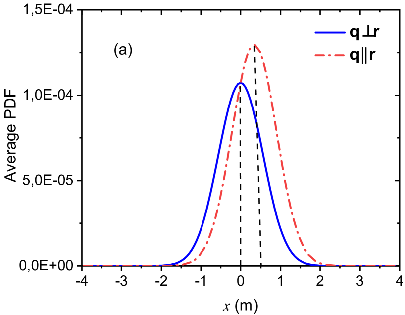
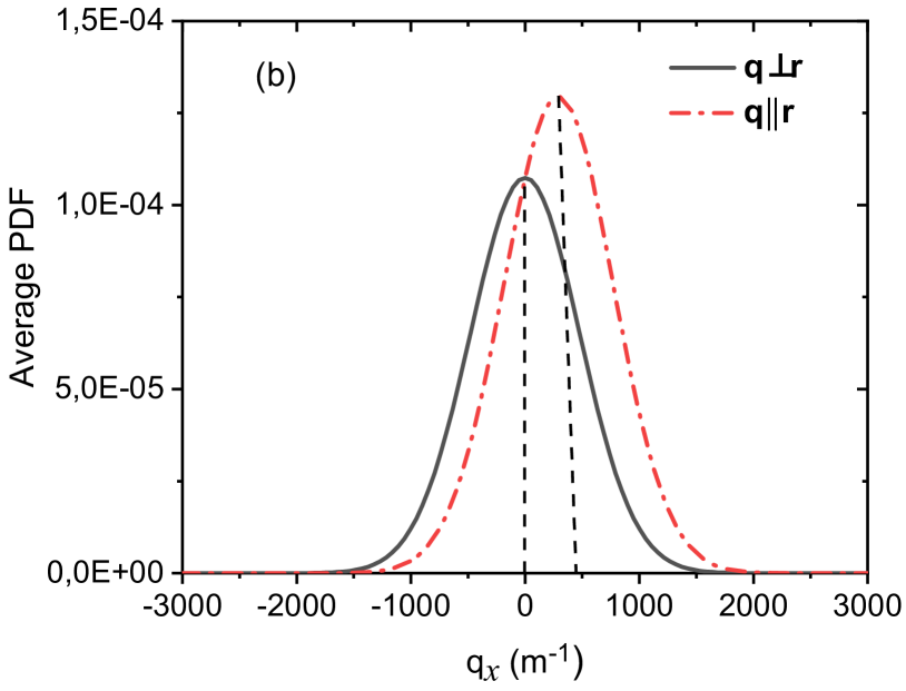
Figure 1: PDF profile in (a) ${\bf r}$-space with fixed $y=0$, $q_{x}=0$, $q_{y}=\sqrt{\alpha t}\equiv\sqrt{\langle{\bf q}^{2}\rangle_{T}}/2$ for solid curve, and $q_{x}=\sqrt{\langle{\bf q}^{2}\rangle_{T}}/2$, $q_{y}=0$ for dash-dotted curve; (b) ${\bf q}$-space with fixed $q_{y}=0$, $x=0$, $y=\sqrt{\frac{z^{3}\alpha}{3q_{0}^{2}c}}\equiv\sqrt{\langle{\bf r}^{2}\rangle_{T}}/2$ for solid curve, and $x=\sqrt{\langle{\bf r}^{2}\rangle_{T}}/2$, $y=0$ for dash-dotted curve. Parameters of the beam and channel: $r_{0}=0.01\,m$, $z=20\,km$, $C_{n}^{2}=2.5\times 10^{-14}\,m^{-2/3}$, $l_{0}/2\pi=10^{-3}\,m$, $q_{0}=10^{7}\,m^{-1}$.

Spatial distribution is symmetric with respect to the direction of ${\bf q}$ and reaches maximum value when ${\bf r}=\frac{{\bf q}ct}{2q_{0}}$ (see Fig. 1). After summing over ${\bf q}$ both sides of the Eq. (IV.3), we obtain the asymptotic value of the photon density,

$$\langle\hat{I}({\bf r},t)\rangle=C\frac{4\pi S}{\langle{\bf r}^{2}\rangle_{T}}e^{-\frac{r^{2}}{\langle{\bf r}^{2}\rangle_{T}}},$$ (46)

which represents the second moment of the radiation field. Then the shot noise, given by the first term in the right side of Eq. (7), reduces to

$$\langle{\delta I}^{2}_{shot}\rangle=C\frac{4\pi S}{\langle{\bf r}^{2}\rangle_{T}}\delta({\bf r}-{\bf r^{\prime}})e^{-\frac{r^{2}}{\langle{\bf r}^{2}\rangle_{T}}}=\langle I({\bf r},t)\rangle\delta({\bf r}-{\bf r^{\prime}}),$$ (47)

where the paraxial approximation was assumed. Equation (47) is the Poissonian-like component of the fourth-order moment derived in Sec. II. In the next Section, the contribution of the shot noise to the full noise is analyzed and interpreted.

V Asymmptotic fourth moment and aperture averaging of fluctuations

The full expression for the fourth moment is obtained after integration of Eq. (46) over ${\bf q}$ and ${\bf q}^{\prime}$. As a result, we get

$$\langle\hat{I}({\bf r},t)\hat{I}({\bf r^{\prime}},t)\rangle=\langle{\delta I}^{2}_{shot}\rangle+\langle\hat{I}({\bf r},t)\rangle\langle\hat{I}({\bf r^{\prime}},t)\rangle+$$

$$\left(\frac{C4\pi S}{\langle{\bf r}^{2}\rangle_{T}}\right)^{2}\exp\left\{{-}\frac{({\bf r}{+}{\bf r^{\prime}})^{2}}{2\langle{\bf r}^{2}\rangle_{T}}{-}\frac{({\bf r}{-}{\bf r^{\prime}})^{2}\langle{\bf q}^{2}\rangle_{T}}{8}\right\},$$ (48)

where the distribution function (IV.3) was used. It is seen from the equation (V) that the characteristic transverse momentum determines the correlation length. This length is of the order of $(8/{{\langle{\bf q}^{2}\rangle}_{T}})^{1/2}$ and decreases with the propagation time as $t^{-1/2}$. Loss of the coherence means that different portions of the radiation field behave independently of each other as non-interacting particles. The long-time asymptotics for the exponential factor in Eq. (V) tends to delta function, the argument of which is the difference of spatial variables [$\sim\delta({\bf r}-{\bf r^{\prime}})$]. Then the last term in (V) can be approximated by

$$\delta({\bf r}-{\bf r}^{\prime})\frac{8\pi}{\langle{\bf q}^{2}\rangle_{T}}\langle I({\bf r},t)\rangle^{2},$$ (49)

where the relation (46) was used. We can now express the full term for the fluctuations of the photon density as

$$\langle\delta\hat{I}({\bf r},t)\delta\hat{I}({\bf r^{\prime}},t)\rangle=\delta({\bf r}-{\bf r}^{\prime})\langle{\hat{I}}({\bf r},t)\rangle\bigg{(}1+\frac{8\pi}{\langle{\bf q}^{2}\rangle_{T}}\langle{\hat{I}}({\bf r},t)\rangle\bigg{)}.$$ (50)

The right side is the sum of the shot noise and the classical noise. The last is quadratic in the radiation density. In the case of high photon density, as one would expect, the classical noise prevails. However, photon density decreases with the increase of distance from the center of the beam, $r$, so the classical component becomes equal to and even less than the shot noise value (47). It is seen from Eq. (50) that the equality occurs for some specific distance $r=r_{q}$ where

$$\langle I({r_{q}},t)\rangle=\frac{\langle{\bf q}^{2}\rangle_{T}}{8\pi}.$$ (51)

The radius ${r_{q}}$ marks the boundary between areas with predominantly ”classical” and ”quantum” fluctuations of light.

The condition (51) can be easily interpreted. The left-hand side describes the two-dimensional density of particles (”photons”). It can be expressed as $\langle I({r_{q}},t)\rangle=a^{-2}$, where $a^{2}$ is a square per particle. On the other hand, the quantity $\langle{\bf q}^{2}\rangle_{T}$ in the right side is equal to $(2\pi/\lambda_{q})^{2}$, where $\lambda_{q}$ is the characteristic wave length of particles in the two-dimensional domain. Using new notations, the condition (51) can be rewritten in a more meaningful form:

$$\lambda_{q}=\sqrt{\frac{\pi}{2}}a.$$ (52)

The value on the left depends on time as $t^{-1/2}$. This means that the increase of propagation time (or propagation distance ${z=ct}$) results in a similar decreasing the size of the ”classical region” $a$. It is possible that for large $t$ the intensity of fluctuations acquires a completely quantum nature at any point of the beam cross-section. The physical picture is opposite to the phenomenon of the Bose condensation. In the process of propagation, classical waves becomes similar to an ensemble of free particles, between which there is no quantum correlation and which can be identified as a two-dimensional gas of non-interacting photons. In other words, the light beam is transformed into the flux of ”free particles”.

At the end of the paragraph, it should be noted that for large (but still finite) values of $\langle{\bf q^{2}}\rangle_{T}$ and small radius of receiving aperture, the $\delta$-function approximation for correlations does not apply. In this case, Eq. (V) should be used. This point is important when the averaging of $\Gamma_{4}$ [see next subsection] occurs in small areas of the $(x,y)$ plane.

Aperture averaging

The asymptotic value for fourth moment can be used to obtain the correlation function of photon density fluctuations averaged over aperture plane of the detector. This physical value is important for measurements because the size of the receiver aperture is always limited vasylyev ; Barrios ; Vetelino . To demonstrate the effect of the receiver aperture $\mathcal{A}$, we utilize intensity transmittance defined by

$$\eta=(4C\pi^{2}S)^{-1}\int\limits_{\mathcal{A}}d{\bf r}\hat{I}({\bf r},t),$$ (53)

where we use normalizing condition $\eta=1$ for $\mathcal{A}$ which is much larger than the beam cross section. The quantity $\eta$ contains both the average and fluctuating constituents and describes transmittance of the optical channel semenov2012 .

Fluctuations of the transmitted radiation are described by the aperture-averaged scintillation index

$$\sigma_{\eta}^{2}=\frac{\langle\eta^{2}\rangle-\langle\eta\rangle^{2}}{\langle\eta\rangle^{2}}.$$ (54)

Two moments for $\eta$ are defined as semenov

$$\langle\eta\rangle = \int\limits_{\mathcal{A}}d{\bf r}\Gamma_{2}({\bf r}),$$ (55)

$$\langle\eta^{2}\rangle = \int\limits_{\mathcal{A}}d{\bf r}\int\limits_{\mathcal{A}}d{\bf r}^{\prime}\Gamma_{4}({\bf r},{\bf r}^{\prime}),$$ (56)

where the normalizing conditions are given by relations: $\Gamma_{2}({\bf r})=\langle\hat{I}({\bf r},t)\rangle/(4C\pi^{2}S)$, $\Gamma_{4}({\bf r},{\bf r}^{\prime})=\langle\hat{I}({\bf r},t)\hat{I}({\bf r^{\prime}},t)\rangle/(4C\pi^{2}S)^{2}$.

For the round receiver aperture with radius $R$ and long-distance propagation we can express moments of transmittance as

$$\langle\eta\rangle = \left(1-\exp\left(-\frac{R^{2}}{\langle{\bf r}^{2}\rangle_{T}}\right)\right),$$ (57)

$$\langle\eta^{2}\rangle{-}\langle\eta\rangle^{2}{=}\int\limits_{0}^{R^{2}}\frac{d\chi}{\langle{\bf r}^{2}\rangle_{T}}\int\limits_{0}^{R^{2}}\frac{d\chi^{\prime}}{\langle{\bf r}^{2}\rangle_{T}}I_{0}\left(\sqrt{\chi\chi^{\prime}}\left(\frac{1}{\langle{\bf r}^{2}\rangle_{T}}{-}\frac{\langle{\bf q}^{2}\rangle_{T}}{4}\right)\right)$$

$$\exp\left(-(\chi{+}\chi^{\prime})\left(\frac{1}{2\langle{\bf r}^{2}\rangle_{T}}{+}\frac{\langle{\bf q}^{2}\rangle_{T}}{8}\right)\right),\hskip 28.45274pt$$ (58)

where $I_{0}$ is modified Bessel function of the first kind. The integral over $\chi^{\prime}$ in Eq. (V) reduces to the incomplete cylindrical function, the analytical approximation of which has been studied in vasylyev2013 .

In the case of large $R$, the delta-correlation approximation (49) can be used. This considerably simplifies the calculation of (56). The result is given by

$$\langle\eta^{2}\rangle{-}\langle\eta\rangle^{2}=\frac{4}{\langle{\bf q}^{2}\rangle_{T}\langle{\bf r}^{2}\rangle_{T}}\left(1-\exp\left(-\frac{2R^{2}}{\langle{\bf r}^{2}\rangle_{T}}\right)\right).$$ (59)

For the realistic set of parameters, two curves are shown in Fig. 2. Both curves agree well only for large values of $R$. In this case, the value of scintillation can be estimated as

$$\sigma_{\eta}^{2}\sim\frac{1}{\langle{\bf q}^{2}\rangle_{T}\langle{\bf r}^{2}\rangle_{T}}\approxeq(\langle{\bf r}^{2}\rangle\langle{\bf q}^{2}\rangle)^{-1}.$$

The same estimate was obtained using the qualitative analysis in Sec. II.

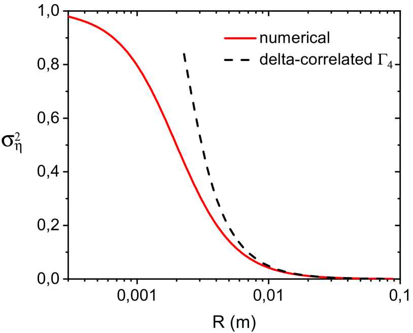
Figure 2: Aperture-averaged scintillation index vs. radius of receiver. Solid line represents the numerical results for (V); dashed line considers delta-correlated behavior of $\Gamma_{4}$, Eq. (59). Parameters of the beam and channel: $z=20\,km$, $C_{n}^{2}=2.5\times 10^{-14}\,m^{-2/3}$, $r_{0}=0.01\,m$, $l_{0}/2\pi=10^{-3}\,m$, $q_{0}=10^{7}\,m^{-1}$.

Numerical calculations illustrate the dependence of aperture-averaged scintillations on the radius of the detector aperture (see Fig. 3). There are two important features of fluctuation transmittance. The first feature relates to the point-like aperture, in which the scintillation index tends to be unity, indicating the effect of saturation of fluctuations (see Sec. II). The second feature is the absence of fluctuations for apertures whose dimensions are much larger than the beam radius.

It can be seen in Fig. 3 that the fluctuation reduction in the asymptotic case strongly depends on the value $\langle{\bf q}^{2}\rangle$. A similar dependence on $R$ was observed in earlier works. This phenomenon was also treated in terms of a coherence length for covariance function Fante3 ; Churnside that is similar to our explanations.

The attempts to study fluctuations of light intensity in the range of of strong turbulence were undertaken by Churnside Churnside and Andrews et al Andrews2 . To our knowledge, the rigorous derivation of analytical expression for $\sigma_{\eta}^{2}$ is given only in the present article.

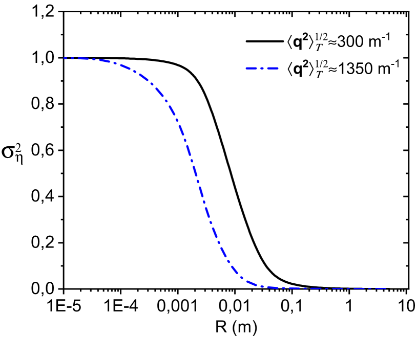
Figure 3: Aperture-averaged scintillation index vs. radius of receiver. Two curves represent propagation in two channels, gaining different change of transverse momenta of photons due to turbulence. Dash-doted line: $z=20\,km$, $C_{n}^{2}=2.5\times 10^{-14}\,m^{-2/3}$; solid line: $z=100\,km$, $C_{n}^{2}=2.5\times 10^{-16}\,m^{-2/3}$. Common parameters of the beam and channel for both curves: $r_{0}=0.01\,m$, $l_{0}/2\pi=10^{-3}\,m$, $q_{0}=10^{7}\,m^{-1}$.

VI Discussion

The coarse-grained photon distribution function, being a specific type of the second moment of the light field, can adequately describe laser beams evolution. It follows from the definition of PDF (1) that the wave-vector ${\bf k}$ describes the spatial distribution of the radiation field. Another wave-vector, ${\bf q}$, describes rather the kinetics of the PDF. There are opposite trends in the evolution of characteristic values of ${\bf k}$ and ${\bf q}$. Spatial and temporal changes correspond to an increase in the radius of the beam (resulting in the decrease of characteristic values of ${\bf k}$) and an increase in the speed of this process over time.

The solution of the averaged kinetic equation for the case of the paraxial beam illustrates the significant anisotropy of the distribution function. The anisotropy is due to photon drift with the velocity $c{\bf q}/q_{0}$ in the direction parallel to the vector ${\bf r}$. It follows from Eq. (IV.3) that the center of spatial distribution of the beam moves with the velocity $c{\bf q}/(2q_{0})$. A simple analytical expression for PDF (IV.3), obtained for long-distance propagation, confirms our interpretation of the results shown in Fig. 1.

The fourth moment describes the intensity of light fluctuations. The corresponding noise level impairs the possibility of using laser beams for practical purposes. At the same time the fourth moment describes the non-local nature of photon fluctuations. This specific property of light is suitable for detailed diagnostics (scanning) of the beam body. Two detectors can be used for this purpose (see Sec II).

By solving the Langevin equation for fluctuating part of the PDF it is possible to obtain the fourth moment. To do this, it is sufficient to find the average of products of the obtained solutions. This program was implemented in our previous paper where a scintillation index was calculated. Unfortunately, the results relate only to weak and moderate turbulence due to the use of iterative procedures there. In the general case, obtaining the fourth moment requires many integrations, which complicates the real calculations. At the same time, the problem simplifies in the case of light propagation over long distances where there is a regime of strong turbulence. Randomization of the transverse momentum coursed by light-eddies collisions changes the statistical properties to those where only pairwise correlations remain.

Using the above reasoning, the fourth moment for fluctuations $\langle\delta\hat{I}({\bf r},t)\delta\hat{I}({\bf r^{\prime}},t)\rangle$ was expressed as the sum of linear and quadratic values of the mean PDF. Linear terms (the shot noise) describe the remote parts of the beam cross-section while the quadratic terms describe the usual (classical) fluctuations of radiations in the central area. The shot noise is the realization of quantum fluctuations. It reveals the discreet nature of light with low intensity (see Sec. V and the article by Kolobov ). It can be interpreted as a noise of non-interacting and non-correlated particles (quasi-particles). The distance where the classical noise becomes equal to quantum noise is obtained analytically in the previous section. It depends on time $t$ and the intensity of radiation.

Explicit fourth moment is used here for obtaining the aperture averaging of fluctuations. The limited aperture of the receiver is typical for most applications, so a rigorous analytical result for transmittance of light fluctuations can be useful. In the asymptotic case, the gain in transverse momentum defines the correlation length for the fourth moment The explicit value of the correlation length can be used for the optimal choice of the detector diameter.

The version of the kinetic equation with the ”collision term” is applicable to almost any propagation distances and strengths of the structure factor $C_{n}^{2}$. An alternative kinetic equation, in which the influence of a turbulence is considered in the framework of the “random force” approach, is analyzed in the Appendix B. It is shown that for long-distance propagation, both approaches give identical results. This is due to relative decrease of the photon momentum transfer in individual photon-eddy collisions (“smooth collisions”).

VII Conclusion

The equation for the average PDF is solved analytically using the Fourier transform in spatial and momentum domains. It is shown that the asymptotic value of the fourth momentum of light field is expressed in terms of linear and quadratic in PDF forms which can be easily calculated. The fourth moment describes the noise level of optical signals and can be used to estimate the performance of optical systems. In particular, they can be used to diagnose optical radiation similar to noise measurements used in the fields of solid state physics and surface science. The results, obtained here, are almost independent on the configuration of the input radiation and could be applied to other optical systems.

VIII Acknowledgments

The authors thank D. Vasylyev, A. Semenov, and E. Stolyarov for useful discussions and comments. The work of R.B. was partially supported by grant(#0120U100155) for Young Scientists Research Laboratories of the National Academy of Sciences of Ukraine.

Appendix A Time dependence in paraxial approximation

When the paraxial beam propagates in the atmosphere, it is possible to replace in the kinetic equation (18) the quantity $ct$ with $z$. To prove this, we multiply both sides of Eq. (18) by $c$, integrate over all values of ${\bf r}_{\bot}$, and sum up over q. As a result, we obtain for $I_{T}(z,t)$, which were introduced in Sec. II, the equation:

$$(\partial_{t}+c\partial_{z})I_{T}(z,t)=0.$$ (60)

There are no dissipative mechanisms in this equation. The total photon flux in the $z$-direction conserves regardless of the atmospheric turbulence. Any function $I_{T}(z-ct)$ satisfies Eq. (60). At the same time, this function must also satisfy the boundary and initial conditions given at $z=0$ and $t=0$. In this particular case equality $I_{T}(z-ct)=I_{T}(0)$ holds and one may conclude that the function $I_{T}(z-ct)$ obeys the initial conditions only if $z=ct$. This property of radiation applies only to cases of paraxial propagation. Our study concerns just this case.

Appendix B Average PDF for Boltzmann collisionless equation

In this Appendix, we consider the applicability of the collisionless Boltzmann kinetic equation for the description of beam propagation. The atmospheric turbulence in this equation is taken into account by substituting expression $-{\bf F}\cdot{\partial_{\bf r}}\hat{f}({\bf r},{\bf q},t)$ instead of $\hat{K}({\bf r},{\bf q},t)-\hat{\nu}_{\bf q}{\hat{f}({\bf r},{\bf q},t)}$ into the right-hand side of (13), we obtain an alternative kinetic equation in which turbulence is manifested by a random force ${\bf F}=\omega_{0}\partial_{\bf r}n({\bf r})$ acting on photons. Such an equation is applicable for description of the range of moderate and strong turbulence (see, for example, Refs. berm ; berm2009 ; baskov2016 ).

$$\{\partial_{t}+{\bf c_{q}}\partial_{\bf r}+{\bf F}({\bf r})\partial_{\bf q}\}\hat{f}({\bf r},{\bf q},t)=0.$$ (61)

Our aim is to solve this equation and compare it with the solution given by Eq. (IV). The general solution of (61) can be written as

$$\hat{f}({\bf r},{\bf q},t)=\phi\bigg{(}{\bf r}-\int_{0}^{t}dt^{\prime}{\bf{\dot{r}}}(t^{\prime});{\bf q}-\int_{0}^{t}dt^{\prime}{\bf{\dot{q}}}(t^{\prime})\bigg{)},$$ (62)

where $\phi({\bf r},{\bf q})$ is the photon distribution function in the aperture plane of the source: $f({\bf r},{\bf q},t=0)=\phi({\bf r},{\bf q})$. In this case, $\phi$ is expressed via the operators $b^{\dagger}_{{\bf q}+\frac{\bf k}{2}},b_{{\bf q}-\frac{\bf k}{2}}$ at $t=0$:

$$\phi({\bf r},{\bf q})=\frac{1}{V}\sum_{\bf k}e^{-i{\bf kr}}(b^{\dagger}_{{\bf q}+\frac{\bf k}{2}}b_{{\bf q}-\frac{\bf k}{2}})|_{t=0}\equiv\sum_{\bf k}e^{-i{\bf kr}}\phi({\bf k},{\bf q}).$$ (63)

Partial integration in Eq. (62) reduces it to

$$\hat{f}({\bf r},{\bf q},t)=\phi\Big{\{}{\bf r}-{\bf c_{q}}t+\frac{c}{q_{0}}\int_{0}^{t}dt^{\prime}t^{\prime}{\bf F}[{\bf r}(t^{\prime})];{\bf q}-\int_{0}^{t}dt^{\prime}{\bf F}[{\bf r}(t^{\prime})]\Big{\}},$$ (64)

where ${\bf c_{q}}$ is the photon velocity at time $t$. It is assumed that the propagation distance $z$ is equal to $ct$ and the fluctuating force ${\bf F}$ as well as trajectories ${\bf r}({\bf q},t^{\prime})$ are perpendicular to the $z$ axis. In this case, the problem reduces to considering the evolution of photons only in the $x,y$ plane.

The explicit form of $\phi({\bf k},{\bf q})$ can be obtained from matching conditions of the source field and the field in the atmosphere. The quantum amplitude $b_{{\bf q}}$ enter to the electromagnetic field via the product $b_{{\bf q}}e^{i{\bf q}\cdot{\bf r}}$. It is assumed that the pattern of source field in the aperture plane is given by function $\Phi({\bf r_{\bot}})$. Therefore, one may write

$$b_{{\bf q_{\bot}},q_{0}}\propto C^{\prime}\int d{\bf r_{\bot}}e^{-i{\bf k_{\bot}r_{\bot}}}\Phi({\bf r_{\bot}}).$$ (65)

Using Eq. (63) and considering $\Phi({\bf r_{\bot}})$ as a Gaussian function $\Phi({\bf r_{\bot}})=const\times e^{-{r^{2}_{\bot}}/r_{0}^{2}}$, we obtain

$$\langle\phi({\bf k},{\bf q})\rangle_{qm}=C^{\prime\prime}e^{-(q_{\bot}^{2}+k_{\bot}^{2}/4)r_{0}^{2}/2},$$ (66)

where the symbol $\langle...\rangle_{qm}$ indicates a quantum-mechanical averaging of operators in the angle brackets. Coefficients $C^{\prime},C^{\prime\prime}$ can be obtained if the total photon flux is known.

Using Eqs. (63),(64) and (66), we find

$$\langle\hat{f}({\bf r_{\bot}},{\bf q_{\bot}},t)\rangle_{qm}=C^{\prime\prime}\sum_{{\bf k}_{\bot}}e^{-i{\bf k_{\bot}R}(t)-Q^{2}(t)r^{2}_{0}/2-k^{2}_{\bot}r^{2}_{0}/8},$$ (67)

where

$${\bf R}(t)={\bf r}_{\bot}-{\bf c_{q}}_{\bot}t+\frac{c}{q_{0}}\int_{0}^{t}dt^{\prime}t^{\prime}{\bf F}[{\bf r_{\bot}}({\bf q_{\bot}},t^{\prime})]$$

and

$${\bf Q}(t)={\bf q_{\bot}}-\int_{0}^{t}dt^{\prime}{\bf F}[{\bf r_{\bot}}({\bf q_{\bot}},t^{\prime})].$$

Further consideration is simplified if we use the identity

$$e^{-Q^{2}r_{0}^{2}/2}=\int\frac{d{\bf p}}{2\pi r_{0}^{2}}e^{-i{\bf pQ}-p^{2}/(2r_{0}^{2})},$$ (68)

where the integration is in the plane $S$. Using Eq. (68) we can exclude $Q^{2}$ in the exponent of the right side of (67). Than we obtain much simpler expression for the distribution in which only one of the exponents contains a linear in F term:

$$\langle\hat{f}({\bf r}_{\bot},{\bf q}_{\bot},t)\rangle_{qm}{=}\frac{C^{\prime\prime}}{2\pi r_{0}^{2}}\sum_{\bf k}\int d{\bf p}e^{-i{\bf k_{\bot}}\{{\bf r}{-}{\bf c_{q}}t\}-i{\bf p}{\bf q}}$$

$$\times e^{-k^{2}r_{0}^{2}/8-p^{2}/2r_{0}^{2}}e^{i\int_{0}^{t}dt^{\prime}\left({\bf p}-{\bf k}\frac{ct^{\prime}}{q_{0}}\right){\bf F}[{\bf r}(t^{\prime})]}.$$ (69)

The last factor in (B) is simplified after averaging over the inhomogeneity of the atmosphere. Assuming the random quantity

$$\Pi={i\int_{0}^{t}dt^{\prime}\left({\bf p}-{\bf k}\frac{ct^{\prime}}{q_{0}}\right){\bf F}[{\bf r}(t^{\prime})]}$$

obeys the Gaussian statistics, we can write

$$\langle e^{\Pi}\rangle=e^{\langle\Pi^{2}\rangle/2}$$ (70)

where

$$\langle\Pi^{2}\rangle=-\frac{8\pi\omega_{0}^{2}}{c}\int_{0}^{t}dt^{\prime}\int d{\bf k^{\prime}_{\bot}}\psi({\bf k^{\prime}_{\bot}})\bigg{[}\bigg{(}{\bf p}-{\bf k_{\bot}}\frac{ct^{\prime}}{q_{0}}\bigg{)}{\cdot}\frac{\bf k^{\prime}_{\bot}}{2}\bigg{]}^{2}.$$ (71)

The following relations were used for obtaining Eq. (71):

$$\langle n({\bf r}_{t^{\prime}})n({\bf r}_{t^{\prime\prime}})\rangle=\int d{\bf k^{\prime}}e^{i{\bf k}^{\prime}_{\bot}({\bf r}_{t^{\prime}}-{\bf r}_{t^{\prime\prime}})-ik^{\prime}_{z}(z^{\prime}-z^{\prime\prime})}\psi_{\bf k^{\prime}}$$

$$\approx\frac{2\pi}{c}\delta(t^{\prime}-t^{\prime\prime})\int d{\bf k^{\prime}}_{\bot}{\psi_{\bf k^{\prime}_{\bot}}},$$ (72)

where $z^{\prime}=ct^{\prime}$,$z^{\prime\prime}=ct^{\prime\prime}$. The use of a delta-function in Eq. (72) becomes possible due to a great difference of photon velocities in the parallel and perpendicular to the propagation path directions: $c\gg cq_{\bot}/q_{0}.$

For long-distance propagation, the sine function included in expression (26) can be replaced by its argument.In this case we have the equivalence of Eqs. (71) and (26):

$$\frac{1}{2}\langle\Pi^{2}\rangle\approx-\gamma({\bf k_{\bot}},{\bf p},t).$$ (73)

Also, the average distribution functions obtained within alternative approaches becomes identical. Therefore the explicit value of the fourth moment (7), can be derived using either of the two.

References

- (1) I. Capraro, A. Tomaello, A. Dall’Arche, F. Gerlin, R. Ursin, G. Vallone, and P. Villoresi, Phys. Rev. Lett. 109, 200502 (2012).
- (2) V. C. Usenko et al., New. J. Phys. 14, 093048 (2012).
- (3) N. Hosseinidehaj and R. Malaney, Phys. Rev. A 91, 022304 (2015).
- (4) M. Aspelmeyer, T. Jennewein, and A. Zeilinger, IEEE Journal of Selected Topics in Quantum Electronics, Vol. 9, Issue 6, 1541 - 1551 (2003).
- (5) X. Ma et al., Nature (London) 489, 269 (2012).
- (6) J.-G. Ren et al., Nature (London) 549, 70 (2017).
- (7) K. Hofmann et al., Phys. Scr. 94, 125104 (2019)
- (8) R. Ursin et al., Nat. Phys. 3, 481 (2007).
- (9) J. Yin et al., Science 356, 1140 (2017).
- (10) C. Peuntinger, B. Heim, C. R. Muller, C. Gabriel, C.Marquardt, and G. Leuchs, Phys. Rev. Lett. 113, 060502 (2014).
- (11) D. Vasylyev, A. A. Semenov, and W. Vogel, Phys. Rev. Lett. 117, 090501 (2016).
- (12) F. Wang, Y. Cai, and O. Korotkova, Proc. SPIE 7588, Atmospheric and Oceanic Propagation of Electromagnetic Waves IV, 75880F (2010).
- (13) D. Shi et al. Opt. Express 21, 2050-2064 (2013).
- (14) V. I. Tatarskii, The effect of the Turbulent Atmosphere on Wave Propagation. (National Technical Information Service, U.S. Department of Commerce, Springfield, VA, 1971).
- (15) R. L. Fante, Proc. IEEE, 63, 1669 (1975).
- (16) R. L. Fante, Proc. IEEE, 68, 1424 (1980), R. L. Fante, Radio Sci. 15, 757 (1980).
- (17) Yu. A. Kravtsov, Rep. Prog. Phys., V. 55, 39, (1992).
- (18) G. P. Berman, A. A. Chumak, and V. N. Gorshkov, Phys. Rev. E, 76, 056606 (2007).
- (19) D. A. DeWolf, J. Opt. Soc. Am. 58, 461-466 (1968).
- (20) G. P. Berman and A. A. Chumak, Phys. Rev. A 74, 013805 (2006).
- (21) G. P. Berman and A. A. Chumak, Phys. Rev. A 79, 063848 (2009).
- (22) O. O. Chumak and R. A. Baskov, Phys. Rev. A, 93, 033821 (2016).
- (23) R. A. Baskov and O. O. Chumak, Phys. Rev. A 97, 043817 (2018).
- (24) Sh. Kogan, Electronic Noise and Fluctuations in Solids (Cambridge University Press, Cambridge, 1996).
- (25) A. A. Tarasenko, P. M. Tomchuk, and A. A. Chumak, Fluctuations in the bulk and on the surface of solids (Naukova Dumka, Kiev, 1992) (in Russian).
- (26) Vellekoop, I.M., Lagendijk, A., Mosk, A.P.Nat. Photonics 4, 320-322 (2010).
- (27) Newman, J.A., Webb, K.J., Phys. Rev. Lett. 113, 263903 (2014).
- (28) Popoff, S.M., Goetschy, A., Liew, S.F., Stone, A.D., Cao, H.: Coherent control of total transmission of light through disordered media.Phys. Rev. Lett. 112, 133903 (2014).
- (29) Vellekoop, I.M., Mosk, A.P., Opt. Lett. bf 32, 2309-2311 (2007).
- (30) O. Katz, E. Smallm Y. Silberberg, Nat. Photonics 6, 549-553 (2012).
- (31) N. D. Hardy and J. H. Shapiro, Phys. Rev. A 87, 023820 (2013).
- (32) P. Zhang, W. Gong, X. Shen, and S. Han, Phys. Rev. A 82, 033817 (2010).
- (33) A. I. Rarenko, A. A. Tarasenko, and A. A. Chumak, Ukr. J. Phys., 37, 1577 (1992), O. Chumak and N. Sushkova, ibid. 57, 30 (2012).
- (34) J. Strohbehn and S. Clifford, IEEE Trans. Antennas Propag., AP-15, 416 (1967).
- (35) L. Mandel and E. Wolf, Optical Coherence and Quantum Optics. Cambridge University, Cambridge (1995).
- (36) M. I. Kolobov, Rev. Mod. Phys., 71, 1539 (1999).
- (37) R. Dashen, J. Math. Phys., 20, 894 (1979).
- (38) Y. Zhang, C. Ding, L. Pan, and Y. Cai, Appl. Sci., 9 , 244 (2019).
- (39) M.O. Scully and M.S. Zubairy, Quantum Optics Cambridge U.P. New York (1996).
- (40) J. Garnier and K. Solna, Arch. Rational Mech. Anal. 220, 37 (2016).
- (41) Probabilistic Analyses and Related Topics, Edited by A. T. Bharucha-Reid, V. 3, Sec. 3, AP 1983.
- (42) Manning R M 1989 Radiative transfer theory for inhomogeneous media with random extinction and scattering coefficients, J. Math. Phys. 30, 2432
- (43) Andrews, L. C. (2004). Field guide to atmospheric optics. Bellingham, WA: SPIE Press.
- (44) Andrews, L. C., Phillips, R. L., and Hopen, C. Y. Waves in Random Media, 10(1), 53-70 (2000).
- (45) D. Vasylyev, W. Vogel, and F. Moll, Phys. Rev. A 99, 053830 (2019).
- (46) R. Barrios, F. Dios, J. Recolons, and A. Rodriguez, Proc. SPIE 7814, Free-Space Laser Communications X, 78140C (2010).
- (47) F. S. Vetelino, C. Young, L. Andrews, and J. Recolons, Appl. Opt. 46, 2099-2108 (2007).
- (48) D. Yu. Vasylyev, A. A. Semenov, and W. Vogel, Phys. Rev. Lett. 108, 220501 (2012).
- (49) D. Vasylyev, W. Vogel, and A. A. Semenov, Phys. Rev. A 97, 063852 (2018).
- (50) D. Vasylyev, A. Semenov, and W. Vogel, Phys. Scr. 2013, 014062 (2013).
- (51) R. L. Fante, J. Opt. Soc. Am. 73, 277-281 (1983).
- (52) J.H. Churnside, Appl. Opt. 30, 1982-94 (1991).
- (53) L C Andrews , R L Phillips and C Y Hopen (2000) Aperture averaging of optical scintillations: power fluctuations and the temporal spectrum, Waves in Random Media, 10:1, 53-70
- (54) Mohammad-Ali Khalighi, Noah Schwartz, Naziha Aitamer, and Salah Bourennane, J. OPT. COMMUN. NETW. ,VOL. 1, NO. 6,NOVEMBER 2009