Approximate and Robust Bounded Job Start Scheduling for Royal Mail Delivery Offices

Abstract

Motivated by mail delivery scheduling problems arising in Royal Mail, we study a generalization of the fundamental makespan scheduling $P||C_{\max}$ problem which we call the bounded job start scheduling problem. Given a set of jobs, each specified by an integer processing time $p_{j}$, that have to be executed non-preemptively by a set of $m$ parallel identical machines, the objective is to compute a minimum makespan schedule subject to an upper bound $g\leq m$ on the number of jobs that may simultaneously begin per unit of time. With perfect input knowledge, we show that Longest Processing Time First (LPT) algorithm is tightly 2-approximate. After proving that the problem is strongly $\mathcal{NP}$-hard even when $g=1$, we elaborate on improving the 2-approximation ratio for this case. We distinguish the classes of long and short instances satisfying $p_{j}\geq m$ and $p_{j}<m$, respectively, for each job $j$. We show that LPT is 5/3-approximate for the former and optimal for the latter. Then, we explore the idea of scheduling long jobs in parallel with short jobs to obtain tightly satisfied packing and bounded job start constraints. For a broad family of instances excluding degenerate instances with many very long jobs, we derive a 1.985-approximation ratio. For general instances, we require machine augmentation to obtain better than 2-approximate schedules. In the presence of uncertain job processing times, we exploit machine augmentation and lexicographic optimization, which is useful for $P||C_{\max}$ under uncertainty, to propose a two-stage robust optimization approach for bounded job start scheduling under uncertainty aiming in a low number of used machines. Given a collection of schedules of makespan $\leq D$, this approach allows distinguishing which are the more robust.We substantiate both the heuristics and our recovery approach numerically using Royal Mail data. We show that, for the Royal Mail application, machine augmentation, i.e. short-term van rental, is especially relevant.

1 Introduction

Royal Mail provides mail collection and delivery services for all United Kingdom (UK) addresses. With a small van fleet (as of January 2019) of 37,000 vehicles and 90,000 drivers delivering to 27 million locations in UK, efficient resource allocation is essential to guarantee the business viability. The backbone of the Royal Mail distribution is a three-layer hierarchical network with 6 regional distribution centers serving 38 mail centers. Each mail center receives, processes, and distributes mail for a large geographically-defined area via 1,250 delivery offices, each serving disjoint sets of neighboring post codes. Mail is collected in mail centers, sorted by region, and forwarded to an appropriate onward mail center, making use of the regional distribution centers for cross-docking purposes. From the onward mail center it is transferred to the final delivery office destination. This process has to be completed within 12 to 16 hours for 1st class post and 24 to 36 hours for 2nd class post depending on when the initial collection takes place.

In a delivery office, post is sorted, divided into routes, and delivered to addresses using a combination of small fleet vans and walked trolleys. Allocating delivery itineraries to vans is critical. Each delivery office has a van exit gate which gives an upper bound the number of vehicles that can depart per unit of time. Thus, we deal with scheduling a set $\mathcal{J}$ of jobs (delivery itineraries), each associated with an integer processing time $p_{j}$, on $m$ parallel identical machines (vehicles), s.t. the makespan, i.e. the last job completion time, is minimized. Parameter $g$ imposes an upper bound on the number of jobs that may simultaneously begin per unit of time. Each job has to be executed non-preemptively, i.e. by a single machine in a continuous time interval without interruptions. We refer to this problem as the Bounded Job Start Scheduling Problem (BJSP).

Our contribution is twofold: First, we derive greedy constant-factor approximation algorithms, i.e. simple heuristics adoptable by Royal Mail practitioners, for effectively solving BJSP instances with perfect knowledge. Second, we propose a two-stage robust optimization approach, based on Royal Mail practices, which evaluates the robustness of BJSP schedules under uncertainty. Using real data, we computationally validate the performance of both the heuristics and two-stage robust optimization approach. Section 1.1 discusses the relationship between BJSP and the fundamental makespan scheduling problem, a.k.a. $P||C_{\max}$. Section 1.2 presents relevant literature. Section 1.3 summarizes the paper’s organization and our contributions.

1.1 Relation to $P||C_{\max}$

(a) Optimal BJSP schedule of makespan $T_{B}=km$.

(b) Optimal $P||C_{\max}$ schedule, without the BJSP constraint, of makespan $T_{M}=k(m+1)/2$.

Figure 1: BJSP instance with $m$ machines, $k$ jobs of processing time $i$, for each $i=1,\ldots,m$, and $g=1$. For an odd number $k=o(m)$, $T_{B}\simeq 2T_{M}$.

With perfect knowledge, BJSP is strongly related to $P||C_{\max}$ which is defined similarly, but drops the BJSP constraint Graham1969 . Broadly speaking, BJSP is harder as a generalization of $P||C_{\max}$ and the two problems become equivalent when $g=m$. $P||C_{\max}$ is strongly $\mathcal{NP}$-hard as a straightforward generation of the 3-Partition problem Garey1979 . The well-known List Scheduling (LS) and Longest Processing Time First (LPT) algorithms achieve tight approximation ratios for $P||C_{\max}$ equal to 2 and 4/3, respectively. Further, $P||C_{\max}$ admits a polynomial-time approximation scheme (PTAS).

Technically, good solutions for both BJSP and $P||C_{\max}$ must attain low imbalance $\max_{i}\{T-T_{i}\}$, where $T$ and $T_{i}$ are the makespan and completion time of machine $i$, respectively. However, BJSP exhibits the additional difficulty of managing and bounding idle machine time during the time interval $[0,\min_{i}\{T_{i}\}]$. To this end, we develop an algorithm that schedules long jobs in parallel with short jobs and bounds idle time with a concave relaxation. Figure 1 shows a job set where the minimum makespan schedules with ($T_{B}$) and without ($T_{M}$) the bounded job start constraint differ by a factor of 2.

Approximate $P||C_{\max}$ solutions can be converted into feasible solutions for BJSP. On the negative side, $P||C_{\max}$ optimal solutions are a factor $\Omega(m)$ from the BJSP optimum, in the worst case. To see this, take an arbitrary $P||C_{\max}$ instance and construct a BJSP one with $g=1$, by adding a large number of unit jobs. The BJSP optimal schedule requires time intervals during which $m-1$ machines are idle at each time, while the $P||C_{\max}$ optimal schedule is perfectly balanced and all machines are busy until the last job completes. On the positive side, we may easily convert any $\rho$-approximation algorithm for $P||C_{\max}$ into a $2\rho$-approximation algorithm for BJSP using naïve bounds. Given that $P||C_{\max}$ admits a PTAS, we obtain an $O(n^{1/\epsilon}\cdot poly(n))$-time $(2+\epsilon)$-approximation algorithm for BJSP. Our main goal is to obtain tighter approximation ratios.

1.2 Related Work

Next, we present related work to designing BJSP approximation algorithms and robust optimization approaches, relevant to Royal Mail delivery offices.

Approximation Algorithms.

BJSP relaxes the scheduling problem with forbidden sets, i.e. non-overlapping constraints, where subsets of jobs cannot run in parallel Schaffter1997 . For the latter problem, better than 2-approximation algorithms are ruled out, unless $\mathcal{P}=\mathcal{NP}$ Schaffter1997 . Even when there is a strict order between jobs in the same forbidden set, the scheduling with forbidden sets problem is equivalent to the precedence-constrained scheduling problem $P|prec|C_{\max}$ and cannot be approximated by a factor lower than $(2-\epsilon)$, assuming a variant of the unique games conjecture Svensson2011 . Also, BJSP relaxes the scheduling with forbidden job start times problem, where no job may begin at certain time points, which does not admit constant-factor approximation algorithms Billaut2009 ; Gabay2016 ; Mnich2018 ; Rapine2013 . Despite the commonalities with the aforementioned literature, to the authors’ knowledge, there is a lack of approximation algorithms for scheduling problems with bounded job starts.

Robust Optimization.

Royal Mail delivery times may be imprecise. Once a delivery has begun, it might finish earlier or later than its anticipated completion time. Because of uncertain job completion times, Royal Mail vans attempting pre-computed schedules may not be able to complete all deliveries during working hours. To this end, robust optimization provides a useful framework for structuring uncertainty, e.g. box uncertainty sets, and incorporating it in the decision-making process BenTal2009 ; Bertsimas2011 ; Goerigk2016 ; Kouvelis2013 . Typically, Royal Mail delivery schedules are computed in two-stages: (i) the first stage computes a feasible, efficient schedule for an initial nominal problem instance before the day begins, and (ii) the second stage recovers the initial schedule by accounting for uncertainty during the day. This setting is naturally captured by two-stage robust optimization with recovery BenTal2004 ; Bertsimas2010 ; Hanasusanto2015 ; Liebchen2009 .

A common way of measuring solution robustness of a given discrete optimization problem instance is by comparing the final solution objective value after uncertainty realization with the solution objective value that we could have achieved if we had a crystal ball that accurately predicts the future. From this perspective, we recently proposed a two-stage robust scheduling approach for $P||C_{\max}$, based on lexicographic optimization Letsios2018 . If processing times are perturbed by a $(1+\epsilon)$ factor, the lexicographic optimization approach yields schedules a factor $(2+O(\epsilon))$ far from achievable optima with perfect knowledge. But this common way of meansuring solution robustness is less applicable for our application because the makespan, i.e. the number of working hours in the day, is fixed. So, in the Royal Mail context, certain decisions can be irrevocable during the recovery process. For Royal Mail delivery offices, job start times can be irrevocable during the day, to reduce delivery delays and overtimes. Further, resource augmentation (or constraint violation), e.g. backup machines, might be essential to ensure the resulting solutions’ feasibility BenTal2000 ; kalyanasundaram2000speed . For this application, we measure a solution’s robustness with the level of resource augmentation, e.g. number of short-term rental vans, required after uncertainty realization. Robust bounded job start scheduling with resource augmentation is an intriguing open question.

1.3 Paper Organization and Contributions

Section 2 formally defines BJSP, proves the problem’s $\mathcal{NP}$-hardness, and derives an $O(\log n)$ integrality gap for a natural integer programming formulation. Section 3 investigates Longest Processing Time First (LPT) algorithm and derives a tight $2$-approximation ratio. We thereafter explore improving this ratio for the special case $g=1$. Section 2 shows that BJSP is strongly $\mathcal{NP}$-hard even when $g=1$. Several of our arguments can be extended to arbitrary $g$, but focusing on $g=1$ avoids many floors, ceilings, and simplifies our presentation. Furthermore, any Royal Mail instance can be converted to $g=1$ using small discretization.

Section 4 distinguishes long versus short instances. An instance $\langle m,\mathcal{J}\rangle$ is long if $p_{j}\geq m$ for each $j\in\mathcal{J}$ and short if $p_{j}<m$ for all $j\in\mathcal{J}$. This distinction comes from the observation that idle time occurs mainly because of (i) simultaneous job completions for long jobs and (ii) limited allowable parallel job executions for short jobs. Section 4 proves that LPT is 5/3-approximate for long instances and optimal for short instances. A key ingredient for establishing the ratio in the case of long instances is a concave relaxation for bounding idle machine time, before the last job start. Section 4 also obtains an improved approximation ratio for long instances, when the maximum job processing time is relatively small, using the Shortest Processing Time First (SPT) algorithm. For long instances, our analysis shows that LPT and SPT achieve low idle machine time after and before, respectively, the last job begins. We leave determining the best trade-off between the two in order to obtain a better approximation ratio as an open question.

Greedy scheduling, e.g. LPT and SPT, which sequences long jobs first and short jobs next, or vice versa, cannot achieve an approximation ratio better than 2. Section 5 proposes Long-Short Mixing (LSM), which devotes a certain number of machines to long jobs and uses all remaining machines for short jobs. By executing the two job types in parallel, LSM reduces the idle time before the last job begins and achieves a 1.985-approximation ratio for a broad family of instances. Carefully bounding idle time before the last job start by accounting for the parallel execution of long jobs with short job starts is the main technical difficulty behind our analysis. For degenerate instances with many very long jobs, we require constant-factor machine augmentation, i.e. $fm$ machines where $f>1$ is constant, to achieve a strictly lower than 2-approximation ratio.

Because Royal Mail delivery scheduling is subject to uncertainty, Section 6 exploits machine augmentation and lexicographic optimization for $P||C_{\max}$ under uncertainty Letsios2018 ; Skutella2016 to construct a two-stage robust optimization approach for the BJSP under uncertainty. We measure robustness based on the resource augmentation required for the final solution feasibility. Our approach distinguishes which among different solutions is more robust. Section 7 substantiates our algorithms and robust optimization approach empirically using Royal Mail data. Section 8 concludes with a collection of intriguing future directions.

2 Problem Definition and Preliminary Results

An instance $I=\langle m,\mathcal{J}\rangle$ of the Bounded Job Start Scheduling Problem (BJSP) is specified by a set $\mathcal{M}=\{1,\ldots,m\}$ of parallel identical machines and a set $\mathcal{J}=\{1,\ldots,n\}$ of jobs. A machine may execute at most one job per unit of time. Job $j\in\mathcal{J}$ is associated with an integer processing time $p_{j}$. Each job should be executed non-preemptively, i.e. in a continuous time interval without interruptions, by a single machine. BJSP parameter $g$ imposes an upper bound on the number of jobs that may begin per unit of time. The goal is to assign each job $j\in\mathcal{J}$ to a machine and decide its starting time so that this BJSP constraint is not violated and the makespan, i.e. the time at which the last job completes, is minimized. Consider a feasible schedule $\mathcal{S}$ with makespan $T$. We denote the start time of job $j$ by $s_{j}$. Each job $j$ must be entirely executed during the interval $[s_{j},C_{j})$, where $C_{j}=s_{j}+p_{j}$ is the completion time of $j$. So, $T=\max_{j\in\mathcal{J}}\{C_{j}\}$. Job $j$ is alive at time $t$ if $t\in[s_{j},C_{j})$. Let $\mathcal{A}_{t}=\{j:[s_{j},C_{j})\cap[t-1,t)\neq\emptyset,j\in\mathcal{J}\}$ and $\mathcal{B}_{t}=\{j:s_{j}\in[t-1,t),j\in\mathcal{J}\}$ be the set of alive and beginning jobs during time unit $t$, respectively. Schedule $\mathcal{S}$ is feasible only if $|\mathcal{A}_{t}|\leq m$ and $|\mathcal{B}_{t}|\leq g$, for all $t$.

BJSP is strongly $\mathcal{NP}$-hard because it becomes equivalent with $P||C_{\max}$ in the special case where $g=\min\{m,n\}$. Theorem 2.1 shows that BJSP is strongly $\mathcal{NP}$-hard also when $g=1$.

Theorem 2.1

BJSP is strongly $\mathcal{NP}$-hard in the special case $g=1$.

Proof

We present an $\mathcal{NP}$-hardness proof from 3-Partition. Given a set $\mathcal{A}=\{a_{1},\ldots,a_{3m}\}$ and a parameter $B\in\mathbb{Z}^{+}$ s.t. $a_{j}\in\mathbb{Z}^{+}$, $B/4\leq a_{j}\leq B/2$, for $j\in\{1,\ldots,3m\}$, and $\sum_{j=1}^{3m}a_{j}=mB$, the 3-Partition problem asks whether there exists a partition of $\mathcal{A}$ into $m$ subsets $\mathcal{S}_{1},\ldots,\mathcal{S}_{m}$ s.t. $\sum_{j\in\mathcal{S}_{i}}a_{j}=B$ for each $i\in\{1,\ldots,m\}$. Given an instance of 3-Partition, construct a BJSP instance $I=\langle m,\mathcal{J}\rangle$ with $n=3m$ jobs of processing time $p_{j}=n^{2}a_{j}$, for $j\in\{1,\ldots,3m\}$, and BJSP parameter $g=1$. W.l.o.g., $n^{2}>3n$. We show that $\mathcal{A}$ admits a 3-Partition iff there exists a feasible schedule $\mathcal{S}$ of makespan $T<n^{2}B+n^{2}$ for $I$.

$\implies$: Suppose that $\mathcal{A}$ admits a 3-Partition $\mathcal{S}_{1},\ldots,\mathcal{S}_{m}$. Because $B/4<a_{j}<B/2$, for $j\in\{1,\ldots,3m\}$, $\mathcal{S}_{i}$ contains exactly three elements, i.e. $|\mathcal{S}_{i}|=3$, for each $i\in\{1,\ldots,m\}$. We fix some arbitrary order $1,\ldots,3m$ of all jobs and construct a schedule $\mathcal{S}$ for $I$ where all jobs in $\mathcal{S}_{i}$ are executed by machine $i\in\mathcal{M}$. The job starting times are decided greedily. In particular, let $T_{i}$ be the last job completion time in machine $i$ just before assigning job $j$. If no job has been assigned to $i$, then $T_{i}=0$. We set $s_{j}$ equal to the earliest time slot after $T_{i}$ at which no job begins in any machine, i.e. $\min\{t:|\mathcal{B}_{t}|<1,t>T_{i}\}$. Now, let $T_{i}$ be the last completion time in machine $i$, once the greedy procedure has been completed. Consider any job $j\in\mathcal{S}_{i}$ and let $j^{\prime}\in\mathcal{S}_{i}$ be the last job executed before $j$ in machine $i$. If no job is executed before $j$, then $s_{j}\leq n$. Otherwise, by construction, we have $|\mathcal{B}_{t}|=1$, for every $t\in[C_{j^{\prime}}+1,s_{j}-1]$. Hence, $s_{j}-C_{j^{\prime}}\leq n-1$. Since $|\mathcal{S}_{i}|=3$ and $|\{t:|\mathcal{B}_{t}|=1,t\in\mathcal{D}\}|\leq n$, we conclude $T_{i}\leq\sum_{j\in\mathcal{S}_{i}}p_{j}+3n=n^{2}\left(\sum_{j\in\mathcal{S}_{i}}a_{j}\right)+3n=n^{2}B+3n<n^{2}B+n^{2}$. So schedule $\mathcal{S}$ attains makespan $T<n^{2}B+n^{2}$.

$\impliedby$: Suppose that there exists a feasible schedule $\mathcal{S}$ of makespan $T<n^{2}B+n^{2}$ for $I$. We argue that each machine executes exactly three jobs. Suppose for contradiction that machine $i\in\mathcal{M}$ executes a subset $\mathcal{S}_{i}$ of jobs with $|\mathcal{S}_{i}|\geq 4$. Denote by $T_{i}=\max\{C_{j}:j\in\mathcal{S}_{i}\}$ the last job completion time in machine $i$. Then, $T_{i}\geq\sum_{j\in\mathcal{S}_{i}}p_{j}=n^{2}\left(\sum_{j\in\mathcal{S}_{i}}a_{j}\right)$. Because $a_{j}\in\mathbb{Z}^{+}$ and $a_{j}>B/4$, it must be the case that $\sum_{j\in\mathcal{S}_{i}}a_{j}\geq B+1$. Hence, $T_{i}\geq n^{2}B+n^{2}$, which is a contradiction on the fact that $T_{i}\leq T$. Thus, schedule $\mathcal{S}$ defines a partitioning of the jobs into $m$ subsets $\mathcal{S}_{1},\ldots,\mathcal{S}_{m}$ s.t. $|\mathcal{S}_{i}|=3$, for each $i\in\mathcal{M}$. We claim that $\sum_{j\in\mathcal{S}_{i}}a_{i}=B$. Otherwise, there would be a machine $i\in\mathcal{M}$ with $\sum_{j\in\mathcal{S}_{i}}a_{i}\geq B+1$ and we would obtain a contradiction using similar reasoning to before. We conclude that $\mathcal{A}$ admits a 3-Partition.

Next, we investigate the integrality gap of a natural integer programming formulation. To obtain this integer program, we partition the time horizon into a set $D=\{1,\ldots,\tau\}$ of unit-length discrete time slots. Time slot $t\in D$ corresponds to time interval $[t-1,t)$. We may naïvely choose $\tau=\sum_{j\in\mathcal{J}}p_{j}$, but smaller $\tau$ values are possible using tighter makespan upper bounds. For simplicity, this manuscript assumes discrete time intervals $[s,t]=\{s,s+1,\ldots,t-1,t\}$, i.e. of integer length. Interval $[1,\tau]$ is the time horizon. In integer programming Formulation (1), binary variables decide a starting time for each job. Binary variable $x_{j,s}$ is 1 if job $j\in\mathcal{J}$ begins at time slot $s\in D$, and 0 otherwise. Continuous variable $T$ corresponds to the makespan. If job $j$ starts at $s$, then it is performed exactly during the time slots $s,s+1,\ldots,s+p_{j}-1$. Hence, job $j$ is alive at time slot $t$ iff it has begun at one among the time slots in the set $A_{j,t}=\{t-p_{j}+1,t-p_{j}+2,\ldots,t\}$. To complete before the time horizon ends, job $j$ must begin at a time slot in the set $F_{j}=\{1,2,\ldots,\tau-p_{j}+1\}$. Finally, denote by $\mathcal{J}_{s}=\{j:s\in\mathcal{F}_{j},j\in\mathcal{J}\}$ the eligible subset of jobs at $s$, i.e. the ones that may be feasibly begin at time slot $s$ without exceeding the time horizon. Formulation (1) models the BJSP problem.

$$\min_{x_{j,s},\;T}\quad T$$ (1a)

$$T\geq x_{j,s}(s+p_{j}) j\in\mathcal{J},s\in D$$ (1b)

$$\sum_{j\in\mathcal{J}}\sum_{\begin{subarray}{c}s\in A_{j,t}\end{subarray}}x_{j,s}\leq m t\in D$$ (1c)

$$\sum_{s\in F_{j}}x_{j,s}=1 j\in\mathcal{J}$$ (1d)

$$\sum_{j\in\mathcal{J}_{s}}x_{j,s}\leq g s\in D$$ (1e)

$$x_{j,s}\in\{0,1\} j\in\mathcal{J},s\in F_{j}$$ (1f)

Expression (1a) minimizes makespan. Constraints (1b) enforce that the makespan is equal to the last job completion time. Constraints (1c) ensure that at most $m$ machines are used at each time slot $t$. Constraints (1d) requires that each job $j$ is scheduled. Constraints (1e) express the BJSP constraint.

Theorem 2.2 shows that the fractional relaxation obtained by replacing Eq. (1f) with the constraints $0\leq x_{j,s}\leq 1$, for $j\in\mathcal{J}$ and $s\in F_{j}$, has a non-constant integrality gap. Thus, stronger linear programming (LP) relaxations are required for obtaining constant-factor approximation algorithms with LP rounding.

Theorem 2.2

The fractional relaxation of integer programming formulation (1) has integrality gap $\Omega(\log n)$.

Proof

Consider an instance with $m$ machines, $n=m$ jobs of processing time $p_{j}=1$ for each $j\in\mathcal{J}$, and BJSP parameter $g=m$. For this instance, the LP solution sets $x_{j,s}=1/(s\cdot\sum_{t=1}^{\tau}\frac{1}{t})$ for each $j,s$. The LP fractional solution is feasible as at each time, no more than $m$ job pieces are feasibly executed (and begin), while the cost is $\max\{sx_{j,s}\}=1/\sum_{t}\frac{1}{t}$. On the contrary, the optimal integral solution has makespan 1.

3 LPT Algorithm

Longest Processing Time first algorithm (LPT) schedules the jobs on a fixed number $m$ of machines w.r.t. the order $p_{1}\geq\ldots\geq p_{n}$. Recall that $|\mathcal{A}_{t}|$ and $|\mathcal{B}_{t}|$ is the number of alive and beginning jobs, respectively, at time slot $t\in D$. We say that time slot $t\in D$ is available if $|\mathcal{A}_{t}|<m$ and $|\mathcal{B}_{t}|<g$. LPT schedules the jobs greedily w.r.t. their sorted order. Each job $j$ is scheduled in the earliest available time slot, i.e. at $s_{j}=\min\{t:|\mathcal{A}_{t}|<m,|\mathcal{B}_{t}|<g,t\in D\}$. Theorem 3.1 proves a tight approximation ratio of 2 for LPT.

Theorem 3.1

LPT is 2-approximate for minimizing makespan and this ratio is tight.

Proof

Denote by $\mathcal{S}$ and $\mathcal{S}^{*}$ the LPT and a minimum makespan schedule, respectively. Let $\ell$ be the job completing last in $\mathcal{S}$, i.e. $T=s_{\ell}+p_{\ell}$. For each time slot $t\leq s_{\ell}$, either $|\mathcal{A}_{t}|=m$, or $|\mathcal{A}_{t}|<m$. Since $\ell$ is scheduled at the earliest available time slot, for each $t\leq s_{\ell}$ s.t. $|\mathcal{A}_{t}|<m$, we have $|\mathcal{B}_{t}|=g$. Let $\lambda$ be the total length of time s.t. $|\mathcal{A}_{t}|<m$ in $\mathcal{S}$. Because of the BJSP constraint, exactly $g$ jobs begin per unit of time, which implies that $\lambda\leq\lceil\frac{\ell}{g}\rceil$. Therefore, schedule $\mathcal{S}$ has makespan:

$$T=s_{\ell}+p_{\ell}\leq\frac{1}{m}\sum_{j\neq\ell}p_{j}+\lambda+p_{\ell}\leq\frac{1}{m}\sum_{j=1}^{n}p_{j}+\left(\left\lceil\frac{\ell}{g}\right\rceil+p_{\ell}\right).$$

Denote by $s_{j}^{*}$ the starting time of job $j$ in $\mathcal{S}^{*}$ and let $\pi_{1},\ldots,\pi_{n}$ the job indices ordered in non-decreasing schedule $\mathcal{S}^{*}$ starting times, i.e. $s_{\pi_{1}}^{*}\leq\ldots\leq s_{\pi_{n}}^{*}$. Because of the BJSP constraint, $s_{\pi_{j}}^{*}\geq\lceil j/g\rceil$. In addition, there exists $j^{\prime}\in[j,n]$ s.t. $p_{\pi_{j^{\prime}}}>p_{j}$. Thus, $\max_{j^{\prime}=j}^{n}\{s_{\pi_{j^{\prime}}^{*}}+p_{\pi_{j^{\prime}}}\}\geq\lceil j/g\rceil+p_{j}$, for $j=1,\ldots,n$. Hence, $\mathcal{S}^{*}$ has makespan:

$$T^{*}\geq\max\left\{\frac{1}{m}\sum_{j=1}^{n}p_{j},\max_{j=1}^{n}\left\{\left\lceil\frac{j}{g}\right\rceil+p_{j}\right\}\right\}.$$

We conclude that $T\leq 2T^{*}$.

(a) LPT schedule of makespan $T\simeq 2mp$.

(b) Optimal schedule of makespan $T^{*}=mp$.

Figure 2: BJSP instance with $g=1$ for the tightness of the LPT 2-approximation ratio, with $m$ machines, $\Theta(m^{2})$ jobs of processing time $p$ and $\Theta(mp)$ unit-length jobs such that $p=\omega(m)$ and $m=\omega(1)$.

Figure 2 illustrates a tightness example of our analysis for LPT. Consider an instance $I=\langle m,\mathcal{J}\rangle$ with $m(m-1)$ long jobs of processing time $p$, where $p=\omega(m)$ and $m=\omega(1)$, $m(p-m)$ unit jobs, and BJSP parameter $g=1$. LPT schedules the long jobs into $m-1$ groups, each one with exactly $m$ . All jobs of a group are executed in parallel for their greatest part. In particular, the $i$-th job of the $k$-th groups is executed by machine $i$ starting at time slot $(k-1)p+i$. All unit jobs are executed sequentially by machine $1$ starting at $(m-1)p+1$. Observe that $\mathcal{S}$ is feasible and has makespan $T=(m-1)p+m(p-m)=(2m-1)p-m^{2}$. The optimal solution $\mathcal{S}^{*}$ schedules all jobs in $m$ groups. The $k$-th group contains $(m-1)$ long jobs and $(p-m+1)$ unit jobs. Specifically, the $i$-th long job is executed by machine $i$ beginning at $(k-1)p+i$, while all short jobs are executed consecutively by machine $m$ starting at $(k-1)p+m$ and completing at $kp$. Schedule $\mathcal{S}^{*}$ is feasible and has makespan $T^{*}=mp$. Because $\frac{m}{p}\rightarrow 0$ and $\frac{1}{m}\rightarrow 0$, i.e. both approach zero, $T\rightarrow 2T^{*}$.

4 Long and Short Instances

This section assumes that $g=1$, but several of the arguments can be extended to arbitrary $g$. From an application viewpoint, any Royal Mail instance can be converted to $g=1$ using small discretization.

4.1 Longest Processing Time First

We consider two natural classes of BJSP instances for which LPT achieves an approximation ratio better than 2. Instance $\langle m,\mathcal{J}\rangle$ is (i) long if $p_{j}\geq m$ for each $j\in\mathcal{J}$ and (ii) short if $p_{j}<m$ for every $j\in\mathcal{J}$. This section proves that LPT is 5/3-approximate for long instances and optimal for short instances. Intuitively, LPT schedules for long instances contain a significant amount of time without job starts, where all machines execute long jobs in parallel. LPT schedules for short instances have no time where all machines simultaneously execute jobs in parallel, because of the BJSP constraint and the fact that all jobs are short. In this case, the number of job starts is significant compared to the overall makespan. Using these observations, we are able to obtain better than 2-approximate schedules for these two classes of instances.

Consider a feasible schedule $\mathcal{S}$ and let $r=\max_{j\in\mathcal{J}}\{s_{j}\}$ be the last job start time. We say that $\mathcal{S}$ is a compact schedule if it holds that either (i) $|\mathcal{A}_{t}|=m$, or (ii) $|\mathcal{B}_{t}|=1$, for each $t\in[1,r]$. Lemma 1 shows the existence of an optimal compact schedule and derives a lower bound on the optimal makespan.

(a) Non-compact schedule.

(b) Compact schedule.

Figure 3: Converting a non-compact schedule to a compact one, by shifting jobs back in increasing order of their starting times.

Lemma 1

For each instance $I=\langle m,\mathcal{J}\rangle$, there exists a feasible compact schedule $\mathcal{S}^{*}$ which is optimal. Let $\mathcal{J}^{L}=\{j:p_{j}\geq m,j\in\mathcal{J}\}$. If $|\mathcal{J}^{L}|\geq m$, then $\mathcal{S}^{*}$ has makespan $T^{*}\geq\frac{1}{m}\left(\frac{m(m-1)}{2}+\sum_{j=1}^{n}p_{j}\right)$.

Proof

For the first part, among the set of all optimal schedules, pick the schedule $\mathcal{S}^{*}$ lexicographically minimizing the vector of job start times sorted in non-decreasing order. We claim that $\mathcal{S}^{*}$ is compact. Assume that this is not the case. Then, there exists a time $t\in[1,r)$ such that $|\mathcal{A}_{t}|<m$ and $|\mathcal{B}_{t}|<1$. Consider the earliest such time $t$. Moreover, let $t^{\prime}$ be the earliest time $t^{\prime}>t$ satisfying either $|\mathcal{A}_{t}|=m$, or $|\mathcal{B}_{t}|=1$. Clearly, there exists a job $j\in\mathcal{J}$ such that $s_{j}=t^{\prime}$. If we decrease the job $j$ start time by one unit of time, we obtain a feasible compact schedule $\mathcal{S^{\prime}}$ with makespan $T^{\prime}\leq T^{*}$, where $T^{*}$ is the schedule $\mathcal{S}^{*}$ makespan, and $\mathcal{S}^{\prime}$ has a lexicographically smaller vector of job start times than $\mathcal{S}^{*}$ which is a contradiction. Figure 3 illustrates how to convert a non-compact schedule to a compact one.

The second part requires lower bounding the total idle machine time $\Lambda=\sum_{t=1}^{r}(m-|\mathcal{A}_{t}|)$ for each feasible schedule $\mathcal{S}$. By the BJSP constraint and the fact that $|\mathcal{J}^{L}|\geq m$, $|\mathcal{B}_{t}|=1$ and, hence, $m-|\mathcal{A}_{t}|\geq m-t$, for each $t\in\{1,\ldots,m\}$. This is because all machines are idle before the first time slot. So, the idle machine during time interval $[1,m]$ is lower bounded by $\Lambda\geq\sum_{t=1}^{m}(m-t)=\frac{m(m-1)}{2}$. A simple packing argument (including both idle and non-idle machine time) implies that schedule $\mathcal{S}$ has makespan $T\geq\frac{1}{m}\left(\frac{m(m-1)}{2}+\sum_{j=1}^{n}p_{j}\right)$.

Next, we analyze LPT in the case of long instances. Similar to the Lemma 1 proof, we may show that LPT produces a compact schedule $\mathcal{S}$. We partition the interval $[1,r]$ into a sequence $P_{1},\ldots,P_{k}$, where $k\leq r$, of maximal periods satisfying the following invariant: for each $q\in\{1,\ldots,k\}$, either (i) $|\mathcal{A}_{t}|<m$ for each $t\in P_{q}$ or (ii) $|\mathcal{A}_{t}|=m$ for each $t\in P_{q}$. That is, there is no pair of time slots $s,t\in P_{q}$ such that $|\mathcal{A}_{s}|<m$ and $|\mathcal{A}_{t}|=m$. We call $P_{q}$ a slack period if $P_{q}$ satisfies (i), otherwise, $P_{q}$ is a full period. For a given period $P_{q}$ of length $\lambda_{q}$, denote by $\Lambda_{q}=\sum_{t\in P_{q}}(m-|\mathcal{A}_{t}|)$ the idle machine time. Note that $\Lambda_{q}=0$, for each full period $P_{q}$. Lemma 2 upper bounds the total idle machine time of slack periods in the LPT schedule $\mathcal{S}$, except the very last period $P_{k}$. When $P_{k}$ is slack, the length $\lambda_{k}$ of $P_{k}$ is upper bounded by Lemma 3.

Lemma 2

Let $k^{\prime}=k-1$. Consider a long instance $I=\langle m,\mathcal{J}\rangle$, with $|\mathcal{J}|\geq m$, and the LPT schedule $\mathcal{S}$. It holds that (i) $\lambda_{q}\leq m-1$ and (ii) $\Lambda_{q}\leq\frac{\lambda_{q}(\lambda_{q}-1)}{2}$ for each slack period $P_{q}$, where $q\in\{1,\ldots,k^{\prime}\}$. Furthermore, (iii) $\sum_{q=1}^{k^{\prime}}\Lambda_{q}\leq\frac{nm}{2}$.

Proof

For (i), let $P_{q}=[s,t]$ be a slack time period in $\mathcal{S}$ and assume for contradiction that $\lambda_{q}\geq m$, i.e. $t\geq s+m-1$. Given that $p_{j}\geq m$ for each $j\in\mathcal{J}$, we have $\{j:s_{j}\in[s,s+m-1],j\in\mathcal{J}\}\subseteq\mathcal{A}_{s+m-1}$. That is, all jobs starting during $[s,s+m-1]$ are alive at time $s+m-1$. Since $P_{q}$ is a slack period, $|\mathcal{A}_{u}|<m$ holds for each $u\in[s,s+m-1]$. Because $\mathcal{S}$ is compact, $|\mathcal{B}_{u}|=1$, i.e. exactly $g=1$ jobs begin, at each $u\in[s,s+m-1]$. This implies $|\mathcal{A}_{s+m-1}|\geq m$, contradicting the fact that $P_{q}$ is a maximal slack period.

For (ii), consider the partitioning $\mathcal{A}_{u}=\mathcal{A}_{u}^{-}+\mathcal{A}_{u}^{+}$ for each time slot $u\in P_{q}=[s,t]$, where $\mathcal{A}_{u}^{-}$ and $\mathcal{A}_{u}^{+}$ is the set of alive jobs at time $u$ completing inside $P_{q}$ and after $P_{q}$, i.e. $C_{j}\in[s,t]$ and $C_{j}>t$, respectively. Since $\lambda_{q}\leq m-1$, every job $j$ beginning during $P_{q}$, i.e. $s_{j}\in[s,t]$, must complete after $P_{q}$, i.e. $C_{j}>t$. We modify schedule $\mathcal{S}$ by removing every job $j$ completing inside $P_{q}$, i.e. $C_{j}\in P_{q}$. Clearly, the modified schedule $\mathcal{S}^{\prime}$ has increased idle time $\Lambda_{q}^{\prime}$ during $P_{q}$, i.e. $\Lambda_{q}\leq\Lambda_{q}^{\prime}$. Further, no job $j$ with $s_{j}\in P_{q}$ is removed. Because $|\mathcal{B}_{u}|=1$ for each $u\in P_{q}$, we have $|\mathcal{A}_{u}|=|\mathcal{A}_{u+1}|-1$ for $u=s,\ldots,t$. Furthermore, $|\mathcal{A}_{t+1}|=m$. So:

$$\Lambda_{q}^{\prime}=\sum_{u=s}^{t}(m-|\mathcal{A}_{u}|)=\sum_{u=s}^{t}[m-(t-s+1)]=\sum_{u=1}^{\lambda_{q}-1}u=\frac{\lambda_{q}(\lambda_{q}-1)}{2}.$$

For (iii), consider slack period $P_{q}$, for $q\in\{1,\ldots,k^{\prime}\}$. By (i), $\lambda_{q}\leq m-1$. Since at most $g=1$ jobs begin at each $t\in P_{q}$, $\sum_{q=1}^{k^{\prime}}\lambda_{q}\leq n-1$. By (ii), Concave Program (2) upper bounds $\sum_{q=1}^{k^{\prime}}\Lambda_{q}$.

$$\max_{\lambda\in\{0,1\}^{k^{\prime}}}\quad \sum_{q=1}^{k^{\prime}}\frac{\lambda_{q}(\lambda_{q}-1)}{2}$$ (2a)

$$1\leq\lambda_{q}\leq m q\in\{1,\ldots,k^{\prime}\}$$ (2b)

$$\sum_{q=1}^{k^{\prime}}\lambda_{q}\leq n$$ (2c)

Assume w.l.o.g. that $n/m$ is integer. If $k^{\prime}\leq n/m$, by setting $\lambda_{q}=m$, for $q\in\{1,\ldots,k^{\prime}\}$, we obtain $\sum_{q=1}^{k^{\prime}}\lambda_{q}(\lambda_{q}-1)/2\leq k^{\prime}m(m-1)/2\leq nm/2$. If $k^{\prime}>n/m$, we argue that the solution $\lambda_{q}=m$, for $q\in\{1,\ldots,n/m\}$, and $\lambda_{q}=0$, otherwise, is optimal for Concave Program (2). In particular, for any solution $\lambda$ with $0<\lambda_{q},\lambda_{q^{\prime}}<m$ such that $q\neq q^{\prime}$, we may construct a modified solution with higher objective value by applying Jensen’s inequality $f(\lambda)+f(\lambda^{\prime})\leq f(\lambda+\lambda^{\prime})$ for any $\lambda,\lambda^{\prime}\in[0,\infty)$, with respect to the single variable, convex function $f(\lambda)=\lambda(\lambda-1)/2$. If $\lambda_{q}+\lambda_{q^{\prime}}\leq m$, we may set $\tilde{\lambda}_{q}=\lambda_{q}+\lambda_{q^{\prime}}$ and $\tilde{\lambda}_{q^{\prime}}=0$. Otherwise, $m<\lambda_{q}+\lambda_{q^{\prime}}\leq 2m$ and we set $\tilde{\lambda}_{q}=m$ and $\tilde{\lambda}_{q^{\prime}}=\lambda_{q}+\lambda_{q^{\prime}}-m$. In both cases, $\lambda_{q^{\prime\prime}}=\tilde{\lambda}_{q^{\prime\prime}}$, for each $q^{\prime\prime}\in\{1,\ldots,k^{\prime}\}\setminus\{q,q^{\prime}\}$. Clearly, $\tilde{\lambda}$ attains higher objective value than $\lambda$, for Concave Program (2).

Lemma 3

Suppose that $P_{k}$ is a slack period and let $\mathcal{J}_{k}$ be the set of jobs beginning during $P_{k}$. Then, it holds that $\lambda_{k}\leq\frac{1}{m}\sum_{j\in\mathcal{J}_{k}}p_{j}$.

Proof

Because $P_{k}$ is a slack period, it must be the case that $|\mathcal{B}_{u}|=1$, for each $u\in P_{k}$. Since we consider long instances, $p_{j}\geq m$ for each $j\in\mathcal{J}$. Therefore, $\lambda_{k}\leq\frac{1}{m}\sum_{j\in\mathcal{J}_{k}}p_{j}$.

Theorem 4.1

LPT achieves an approximation ratio $\rho\in\left[\frac{3}{2},\frac{5}{3}\right]$ in the case of long instances.

Proof

Denote the LPT and optimal schedules by $\mathcal{S}$ and $\mathcal{S}^{*}$, respectively. Let $\ell\in\mathcal{J}$ be a job completing last in $\mathcal{S}$, i.e. $T=s_{\ell}+p_{\ell}$. Recall that LPT sorts jobs s.t. $p_{1}\geq\ldots\geq p_{n}$. W.l.o.g. we assume that $\ell=\arg\min_{j\in\mathcal{J}}\{p_{j}\}$. Indeed, we may discard every job $j>\ell$ and bound the algorithm’s performance w.r.t. instance $\tilde{I}=\langle m,\mathcal{J}\setminus\{j:j>\ell,j\in\mathcal{J}\}\rangle$. Let $\tilde{S}$ and $\tilde{S}^{*}$ be the LPT and an optimal schedule attaining makespan $\tilde{T}$ and $\tilde{T}^{*}$, respectively, for instance $\tilde{I}$. Showing that $\tilde{T}\leq(5/3)\tilde{T}^{*}$ is sufficient for our purposes because $T=\tilde{T}$ and $\tilde{T}^{*}\leq T^{*}$. We distinguish two cases based on whether $p_{n}>T^{*}/3$, or $p_{n}\leq T^{*}/3$.

Case 1 ($p_{n}>T^{*}/3$): We claim $T\leq(3/2)T^{*}$. Initially, observe that $n\leq 2m$. Otherwise, there would be a machine $i\in\mathcal{M}$ executing at least $|\mathcal{S}_{i}^{*}|\geq 3$ jobs, say $j,j^{\prime},j^{\prime\prime}\in\mathcal{J}$, in $\mathcal{S}^{*}$. This machine would have last job completion time $T_{i}^{*}\geq p_{j}+p_{j^{\prime}}+p_{j^{\prime\prime}}>T^{*}$, a contradiction. If $n\leq m$, LPT clearly has makespan $T=T^{*}$. So, consider $n>m$. Then, some machine executes at least two jobs in $\mathcal{S}^{*}$, i.e. $p_{n}\leq T^{*}/2$. To prove our claim, it suffices to show $s_{n}\leq T^{*}$, i.e. job $n$ starts before or at $T^{*}$. Let $c=\max_{1\leq j\leq m}\{C_{j}\}$ be the time when the last among the $m$ biggest jobs completes. If $s_{n}\leq c$, then $s_{n}\leq\max_{1\leq j\leq m}\{j+p_{j}\}\leq T^{*}$. Otherwise, let $\lambda=s_{n}-c$. Because $n\leq 2m$, it must be the case that $\lambda\leq m$. Furthermore, $|\mathcal{A}_{t}|<m$ and, thus, $|\mathcal{B}_{t}|=1$, for each $t\in[c+1,s_{n}-1]$. That is, exactly one job begins per unit of time during $[c+1,s_{n}]$. Due to the LPT ordering, these are exactly the jobs $\{n-\lambda,\ldots,n\}$. Since $\lambda\leq m$ and $p_{j}\geq m$, at least $m-h$ units of time of job $n-h$ are executed from time $s_{n}$ and onwards, for $h\in\{1,\ldots,\lambda\}$. Thus, the total processing load which executed not earlier than $s_{n}$ is $\mu\geq\sum_{h=1}^{\lambda}(m-h)$. On the other hand, at most $m-h$ machines are idle at time slot $c+h$, for $h\in\{1,\ldots,\lambda\}$. So, the total idle machine time during $[m+1,s_{n}-1]$ is $\Lambda\leq\sum_{h=1}^{\lambda-1}(m-h)$. We conclude that $\mu\geq\Lambda$ which implies that $s_{n}\leq\frac{m(m-1)}{2}+\frac{1}{m}\sum_{j\in\mathcal{J}}p_{j}$. By Lemma 1, our claim follows.

Case 2 ($p_{n}\leq T^{*}/3$): In the following, Equalities (3a) hold because job $n$ completes last and by the definition of alive jobs. Inequalities (3b)-(3d) use a simple packing argument with job processing times and machine idle time taking into account: (3b) Lemma 3, (3c) Lemma 2 property $\sum_{q=1}^{k^{\prime}}\Lambda_{q}\leq\frac{nm}{2}$, and (3d) the bound $T^{*}\geq\max\{\frac{1}{m}\sum_{j\in\mathcal{J}}p_{j},n+p_{n},3p_{n}\}$.

$$T =s_{n}+p_{n}=\frac{1}{m}\left(\sum_{t=1}^{s_{n}}|\mathcal{A}_{t}|+\sum_{t=1}^{s_{n}}\left(m-|\mathcal{A}_{t}|\right)\right)+p_{n}$$ (3a)

$$\leq\frac{1}{m}\left(\sum_{i=1}^{n}p_{i}+\sum_{q=1}^{k^{\prime}}\Lambda_{q}\right)+p_{n}$$ (3b)

$$\leq\frac{1}{m}\sum_{i=1}^{n}p_{i}+\frac{n}{2}+p_{n}$$ (3c)

$$\leq\frac{5}{3}T^{*}.$$ (3d)

(a) LPT schedule of makespan $T=3m-1$.

(b) Optimal schedule of makespan $T^{*}=2m$.

Figure 4: BJSP long instance with a 3/2 lower bound of LPT.

We complement Theorem 4.1 with a long instance $I=\langle m,\mathcal{J}\rangle$ where LPT is 3/2-approximate and leave closing the gap between the two as an open question. Instance $I$ is illustrated in Figure 4 and contains $m+1$ jobs, where $p_{j}=2m-j$, for $j\in\{1,\ldots,m\}$, and $p_{m+1}=m$. In the LPT schedule $\mathcal{S}$, job $j$ is executed at time $s_{j}=j$, for $j\in\{1,\ldots,m\}$, and $s_{m+1}=2m-1$. Hence, $T=3m-1$. But an optimal schedule $\mathcal{S}^{*}$ assigns job $j$ to machine $j+1$ at time $s_{j}=j+1$, for $j\in\{1,\ldots,m-1\}$. Moreover, jobs $m$ and $m+1$ are assigned to machine $1$ beginning at times $s_{m}=1$ and $s_{m+1}=m$, respectively. Clearly, $\mathcal{S}^{*}$ has makespan $T^{*}=2m$.

Theorem 4.2 completes this section with a simple argument on the LPT performance for short instances.

Theorem 4.2

LPT is optimal for short instances.

Proof

Let $p_{1}\geq\ldots\geq p_{n}$ be the LPT job ordering and suppose that job $\ell$ completes last in LPT schedule $\mathcal{S}$. We claim that job $\ell$ begins at time slot $s_{\ell}=\lceil\ell/g\rceil$ in $\mathcal{S}$. Due to the BJSP constraint, we have $s_{\ell}\geq\lceil\ell/g\rceil$. Assume that the last inequality is strict. Then, $|\mathcal{A}_{t}|=m$ for some time slot $t<s_{\ell}$. So, there exists job $j\in\mathcal{A}_{t}$ with $s_{j}=t-m+1$. Since $p_{j}\leq m-1$, we get $C_{j}<t$ which contradicts $j\in\mathcal{A}_{t}$. Because $T^{*}\geq\lceil j/g\rceil+j$ for each $j\in\mathcal{J}$, the theorem follows.

4.2 Shortest Processing Time First

This section investigates the performance of Long Job Shortest Processing Time First Algorithm (LSPT). LSPT orders the jobs as follows: (i) each long job precedes every short job, (ii) long jobs are sorted according to Shortest Processing Time First (SPT), and (iii) short jobs are sorted as in LPT. LSPT schedules jobs greedily, in the same vein as LPT, with this new job ordering. For long instances, when the largest processing time $p_{\max}$ is relatively small compared to the average machine load, Theorem 4.3 shows that LSPT achieves an approximation ratio better than the 5/3, i.e. the approximation ratio Theorem 4.1 obtains for LPT. From a worst-case analysis viewpoint, the main difference between LSPT and LPT is that the former requires significantly lower idle machine time until the last job start, but at the price of much higher difference between the last job completion times in different machines.

Theorem 4.3

LSPT is 2-approximate for minimizing makespan. For long instances, LSPT is $(1+\min\{1,1/\alpha\})$-approximate, where $\alpha=(\frac{1}{m}\sum_{j\in\mathcal{J}}p_{j})/p_{\max}$.

Proof

Let $\mathcal{S}$ be the LSPT schedule and suppose that it attains makespan $T$. Moreover, denote by $\ell\in\mathcal{S}$ the job completing last, i.e. $C_{\ell}=T$. Similarly to the Lemma 1 proof, $\mathcal{S}$ is compact. We distinguish two cases based on whether $|\mathcal{J}^{L}|<m$, or $|\mathcal{J}^{L}|\geq m$. In the former case, every job $j\in\mathcal{J}^{L}$ satisfies $s_{j}\leq p_{\max}$. Using similar reasoning to the Theorem 3.1 proof, we get $T\leq p_{\max}+n+p_{\min}$.

In latter case, let $t^{\prime}=\min\{t:|\mathcal{A}_{t}|<m,t>m\}$. That is, $t^{\prime}$ is the earliest time slot strictly after time $t=m$ when at least one machine is idle. We claim that $s_{j}<t^{\prime}$ for each $j\in\mathcal{J}^{L}$, i.e. every long job begins before $t^{\prime}$ and there is no idle machine time during $[m,t^{\prime}]$. Assume for contradiction that there is some job $j\in\mathcal{J}^{L}$ such that $s_{j}>t^{\prime}$. Since, there is an idle machine at $t^{\prime}$ and long jobs remain to begin after $t^{\prime}$, at least two jobs $j^{\prime},j^{\prime\prime}\in\mathcal{J}^{L}$ complete simultaneously at $t^{\prime}-1$, i.e. $C_{j^{\prime}}=C_{j^{\prime\prime}}=t^{\prime}-1$. Because of the BJSP constraint $|\mathcal{B}_{t}|\leq 1$, it must by the case that $s_{j^{\prime}}\neq s_{j^{\prime\prime}}$. W.l.o.g. $s_{j^{\prime}}<s_{j^{\prime\prime}}$. By the SPT ordering, we also have that $p_{j^{\prime}}\leq p_{j^{\prime\prime}}$. Thus, we get the contradiction $C_{j^{\prime}}<C_{j^{\prime\prime}}$. Our claim implies that $t^{\prime}\leq\frac{m(m-1)}{2}+\frac{1}{n}\sum_{j\in\mathcal{J}}p_{j}$.

Next, consider two subcases based on whether $\ell\in\mathcal{J}^{L}$, or $\ell\in\mathcal{J}^{S}$. If $\ell\in\mathcal{J}^{L}$, then $T\leq t^{\prime}+p_{\max}$. Otherwise, if $\ell\in\mathcal{J}^{S}$, then $T\leq t^{\prime}+n+p_{\min}$. In both subcases,

$$T\leq\frac{m(m-1)}{2}+\frac{1}{n}\sum_{j=1}^{n}p_{j}+\max\left\{p_{\max},n+p_{\min}\right\}.$$

Obviously, the optimal solution satisfies:

$$T^{*}\geq\max\left\{\frac{1}{m}\sum_{j=1}^{n}p_{j},p_{\max},n+p_{\min}\right\}.$$

In all cases, $T\leq 2T^{*}$. For long instances, i.e. the case $\ell\in\mathcal{J}^{L}$, LSPT is $(1+\min\{1,1/\alpha\})$-approximate.

5 Parallelizing Long and Short Jobs

This section proposes the Long Short Job Mixing Algorithm (LSM) to compute 1.985-approximate schedules for a broad family of instances, e.g. with at most $\lceil 5m/6\rceil$ jobs of processing time (i) $p_{j}>(1-\epsilon)(\sum_{j^{\prime}}p_{j^{\prime}})$, or (ii) $p_{j}>(1-\epsilon)(\max_{j^{\prime}}\{j^{\prime}+p_{j^{\prime}}\})$ assuming non-increasing $p_{j}$’s, for sufficiently small constant $\epsilon>0$. For degenerate instances with more than $\lceil 5m/6\rceil$ jobs of processing time $p_{j}>T^{*}/2$, where $T^{*}$ is the optimal objective value, LSM requires constant machine augmentation to achieve an approximation ratio lower than 2. There can be at most $m$ such jobs. In the Royal Mail application, machine augmentation davis2011survey ; kalyanasundaram2000speed ; phillips2002optimal adds more delivery vans. For simplicity, we also assume that $m=\omega(1)$, but the approximation ratio can be adapted for smaller values of $m$. However, we require that $m\geq 7$.

Figure 5: Structure of schedules produced by LSM. Long jobs are prioritized in the subset $\mathcal{M}^{L}$ of the machines. The subset $\mathcal{M}^{S}$ of remaining machines execute only short jobs.

LSM attempts to construct a feasible schedule where long jobs are executed in parallel with short jobs, as depicted in Figure 5. LSM uses $m^{L}<m$ machines for executing long jobs. The remaining $m^{S}=m-m^{L}$ machines are reserved for short jobs. Carefully selecting $m^{L}$ allows to obtain a good trade-off in terms of (i) delaying long jobs and (ii) achieving many short job starts at time slots when many long jobs are executed in parallel. Here, we set $m^{L}=\lceil 5m/6\rceil$. Before formally presenting LSM, we modify the notions of long and short jobs by setting $\mathcal{J}^{L}=\{j:p_{j}\geq m^{L},j\in\mathcal{J}\}$ and $\mathcal{J}^{S}=\{j:p_{j}<m^{L},j\in\mathcal{J}\}$, respectively. Both $\mathcal{J}^{L}$ and $\mathcal{J}^{S}$ are sorted in non-increasing processing time order. LSM schedules jobs greedily by traversing time slots in increasing order. Let $\mathcal{A}_{t}^{L}$ be the set of alive long jobs at time slot $t\in D$. For $t=1,\ldots,\tau$, LSM proceeds as follows: (i) if $|\mathcal{A}_{t}^{L}|<m^{L}$, then the next long job begins at $t$, (ii) if $|J^{L}|=0$ or $m^{L}\leq|\mathcal{A}|<m$, LSM schedules the next short job to start at $t$, else (iii) LSM considers the next time slot. From a complementary viewpoint, LSM partitions the machines $\mathcal{M}$ into $\mathcal{M}^{L}=\{i:i\leq m^{L},i\in\mathcal{M}\}$ and $\mathcal{M}^{S}=\{i>m^{L},i\in\mathcal{M}\}$. LSM prioritizes long jobs on machines $\mathcal{M}^{L}$ and assigns only short jobs to machines $\mathcal{M}^{S}$. A job may undergo processing on machine $i\in\mathcal{M}^{S}$ only if all machines in $\mathcal{M}^{L}$ are busy. The Algorithm 1 pseudocode describes LSM.

Algorithm 1 Long-Short Mixing (LSM)

Sort $\mathcal{J}^{L}=\{j\in\mathcal{J}:p_{j}\geq m^{L}\}$ in non-increasing order.

Sort $\mathcal{J}^{S}=\{j\in\mathcal{J}:p_{j}<m^{L}\}$ in non-increasing order.

for $t=1,\ldots,\tau$ do

     if $|\mathcal{A}_{t}|<m$ then

         if $|\mathcal{A}_{t}^{L}|<m^{L}$ and $|\mathcal{J}^{L}|>0$ then

              $j^{\prime}=\arg\max_{j\in\mathcal{J}^{L}}\{p_{j}\}$

              $\mathcal{J}^{L}=\mathcal{J}^{L}\setminus\{j^{\prime}\}$

         else if $|\mathcal{J}^{S}|>0$ then

              $j^{\prime}=\arg\max_{j\in\mathcal{J}^{S}}\{p_{j}\}$

              $\mathcal{J}^{S}=\mathcal{J}^{S}\setminus\{j^{\prime}\}$          

         In either of the above cases, set $s_{j^{\prime}}=t$.      

Theorem 5.1 shows that LSM achieves a better approximation ratio than LPT, i.e. strictly lower than 2, for a broad family of instances.

Theorem 5.1

LSM is 1.985-approximate (i) for instances with no more than $\lceil 5m/6\rceil$ jobs s.t. $p_{j}>(1-\epsilon)\max\{\frac{1}{m}\sum_{j^{\prime}}p_{j^{\prime}},\max_{j^{\prime}}\{j^{\prime}+p_{j^{\prime}}\}\}$ for sufficiently small $\epsilon>0$, and (ii) for general instances using 1.2-machine augmentation.

Proof

Let $\mathcal{S}$ be the LSM schedule and $\ell=\arg\max\{C_{j}:j\in\mathcal{J}\}$ the job completing last. That is, $\mathcal{S}$ has makespan $T=C_{\ell}$. For notational convenience, given a subset $P\subseteq D$ of time slots, denote by $\lambda(P)=|P|$ and $\mu(P)=\sum_{t\in P}|\mathcal{A}_{t}|$ the number of time slots and executed processing load, respectively, during $P$. Furthermore, let $n^{L}=|\mathcal{J}^{L}|$ and $n^{S}=|\mathcal{J}^{S}|$ be the number of long and short jobs, respectively. We distinguish two cases based on whether (i) $\ell\in\mathcal{J}^{S}$ or (ii) $\ell\in\mathcal{J}^{L}$.

Case $\ell\in\mathcal{J}^{S}$

We partition time slots $\{1,\ldots,T\}$ into five subsets. Let $r^{L}=\max_{j\in\mathcal{J}^{L}}\{s_{j}\}$ and $r^{S}=\max_{j\in\mathcal{J}^{S}}\{s_{j}\}$ be the maximum long and short job start time, respectively, in $\mathcal{S}$. Since $\ell\in\mathcal{J}^{S}$, it holds that $r^{L}<r^{S}$. For each time slot $t\in[1,r^{L}]$ in $\mathcal{S}$, either $|\mathcal{A}_{t}^{L}|=m^{L}$ long jobs simultaneously run at $t$, or not. In the latter case, it must be the case that $t=s_{j}$ for some $j\in\mathcal{J}^{L}$. On the other hand, for each time slot $t\in[r^{L}+1,s_{\ell}]$, either $|\mathcal{A}_{t}|=m$, or $t=s_{j}$ for some $j\in\mathcal{J}^{S}$. Finally, $[s_{\ell},T(\mathcal{S})]$ is exactly the interval during which job $\ell$ is executed. Then, we may define:

• $F^{L}=\{t:|\mathcal{A}_{t}^{L}|=m^{L}\}$,

• $B^{L}=\{t:|\mathcal{A}_{t}^{L}|<m^{L},t=s_{j},j\in\mathcal{J}^{L}\}$,

• $F^{S}=\{t:t>r^{L},|\mathcal{A}_{t}|=m\}$, and

• $B^{S}=\{t:t>r^{L},|\mathcal{A}_{t}|<m,t=s_{j},j\in\mathcal{J}^{S}\}$.

Clearly,

$$T\leq\lambda(F^{L})+\lambda(B^{L})+\lambda(F^{S})+\lambda(B^{S})+p_{\ell}.$$ (4)

Next, we upper bound a linear combination of $\lambda(F^{L})$, $\lambda(B^{S})$, and $\lambda(F^{S})$ taking into account the fact that certain short jobs begin during a subset $\hat{B}^{S}\subseteq F^{L}\cup F^{S}$ of time slots. By definition, $\lambda(B^{S})\leq n^{S}-\lambda(\hat{B}^{S})$. We claim that $\lambda(\hat{B}^{S})\geq(m^{S}/m^{L})(\lambda(F^{L})+\lambda(F^{S}))$. For this, consider the time slots $F^{L}\cup F^{S}$ as a continuous time period by disregarding intermediate $B^{L}$ and $B^{S}$ time slots. Partition this $F^{L}\cup F^{S}$ time period into subperiods of equal length $m^{L}$. Note that no long job begins during $F^{L}\cup F^{S}$ and the machines in $\mathcal{M}^{S}$ may only execute small jobs in $\mathcal{S}$. Because of the greedy nature of LSM and the fact that $p_{j}<m^{L}$ for $j\in\mathcal{J}^{S}$, there are at least $m^{S}$ short job starts in each subperiod. Hence, our claim is true and we obtain that $\lambda(B^{S})\leq n^{S}-(m^{S}/m^{L})(\lambda(F^{L})+\lambda(F^{S}))$, or equivalently:

$$m^{S}\lambda(F^{L})+m^{S}\lambda(F^{S})+m^{L}\lambda(B^{S})\leq m^{L}n^{S}.$$ (5)

Subsequently, we upper bound a linear combination of $\lambda(F^{L})$, $\lambda(B^{L})$, and $\lambda(F^{S})$ using a simple packing argument. The part of the LSM schedule for long jobs is exactly the LPT schedule for a long instance with $n^{L}$ jobs and $m^{L}$ machines. If $|\mathcal{A}_{r^{L}}^{L}|<m$, we make the convention that $\mu(B^{L})$ does not contain any load of jobs beginning in the maximal slack period completed at time $r^{L}$. Observe that $\mu(F^{L})=m^{L}\lambda(F^{L})$ and $\mu(F^{S})=m\lambda(F^{S})$. Additionally, by Lemma 2, we get that $\mu(B^{L})\geq m^{L}\lambda(B^{L})/2$, except possibly the very last slack period. Then, $\mu(F^{L})+\mu(B^{L})+\mu(F^{S})\leq\sum_{j\in J}p_{j}$. Hence, we obtain:

$$m^{L}\lambda(F^{L})+\frac{1}{2}m^{L}\lambda(B^{L})+m\lambda(F^{S})\leq\sum_{j\in\mathcal{J}}p_{j}.$$ (6)

Summing Expressions (5) and (6),

$$\left(m^{L}+m^{S}\right)\lambda(F^{L})+\frac{1}{2}m^{L}\lambda(B^{L})+\left(m+m^{S}\right)\lambda(F^{S})+m^{L}\lambda(B^{S})\leq\sum_{j\in\mathcal{J}}p_{j}+m^{L}n^{S}.$$

Because $m=m^{L}+m^{S}$, if we divide by $m$, the last expression gives:

$$\lambda(F^{L})+\frac{1}{2}\left(\frac{m^{L}}{m^{\phantom{L}}}\right)\lambda(B^{L})+\lambda(F^{S})+\left(\frac{m^{L}}{m^{\phantom{L}}}\right)\lambda(B^{S})\leq\frac{1}{m}\sum_{j\in\mathcal{J}}p_{j}+\left(\frac{m^{L}}{m^{\phantom{L}}}\right)n^{S}.$$ (7)

We distinguish two subcases based on whether $\lambda(F^{S})+\lambda(F^{L})\geq 5n^{S}/6$ or not. Obviously, $\lambda(B^{L})\leq n^{L}$. In the former subcase, Inequality (5) gives $\lambda(B^{S})\leq(1-\frac{5m^{S}}{6m^{L}})n^{S}$. Using Inequality (7), Expression (4) becomes:

$$T \leq\frac{1}{m}\sum_{j\in\mathcal{J}}p_{j}+\left(1-\frac{m^{L}}{2m}\right)n^{L}+\left[\left(\frac{m^{L}}{m^{\phantom{L}}}\right)+\left(1-\frac{m^{L}}{m^{\phantom{L}}}\right)\left(1-\frac{5m^{S}}{6m^{L}}\right)\right]n^{S}+p_{\ell}.$$

For $m^{L}=\lceil 5m/6\rceil$, we have (i) $5/6\leq m^{L}/m\leq 5/6+1/m$ and (ii) $m^{S}/m^{L}\geq\frac{1/6-1/m}{5/6+1/m}$. Given $m=\omega(1)$,

$$T \leq\frac{1}{m}\sum_{j\in\mathcal{J}}p_{j}+\left(1-\frac{5}{12}\right)n^{L}+\left[\frac{5}{6}+\left(1-\frac{5}{6}\right)\left(1-\frac{1}{5}\right)\right]n^{S}+p_{\ell}.$$

Note that an optimal solution $\mathcal{S}^{*}$ has makespan:

$$T^{*}\geq\max\left\{\frac{1}{m}\sum_{j\in\mathcal{J}}p_{j},n^{L}+n^{S}+p_{\ell}\right\}.$$

Because the instance is mixed with long and short jobs and we consider the case $\ell\in\mathcal{J}^{S}$, we have $p_{\ell}\geq T^{*}/2$. Therefore, $T\leq(1+\frac{29}{30}+(\frac{29}{30})\frac{1}{2})T^{*}\leq 1.985T^{*}$. Now, consider the opposite subcase where $\lambda(F^{L})+\lambda(F^{S})\leq 5n^{S}/6$. Given $\lambda(B^{L})\leq n^{L}$ and $\lambda(B^{S})\leq n^{S}$, expression (4) becomes $T\leq\frac{11}{6}(n^{S}+n^{L}+p_{\ell})\leq 1.835\cdot T^{*}$.

Case $\ell\in\mathcal{J}^{L}$

Recall that $\mathcal{A}_{t}^{L}$ and $\mathcal{B}_{t}^{L}$ are the sets of long jobs which are alive and begin, respectively, at time slot $t$. Furthermore, $r^{L}=\max\{s_{j}:j\in\mathcal{J}^{L}\}$ is the last long job starting time. Because LSM greedily uses $m^{L}$ machines for long jobs, either $|\mathcal{A}_{t}^{L}|=m^{L}$, or $|\mathcal{B}_{t}^{L}|=1$, for each $t\in[1,r^{L}]$. So, we may partition time slots $\{1,\ldots,r^{L}\}$ into $F^{L}=\{t:|\mathcal{A}_{t}^{L}|=m\}$ and $B^{L}=\{t:|\mathcal{A}_{t}^{L}|<m,|\mathcal{B}_{t}^{L}|=1\}$ and obtain:

$$T\leq\lambda(F^{L})+\lambda(B^{L})+p_{\ell}.$$

Because $m^{L}$ long jobs are executed at each time slot $t\in F^{L}$,

$$\lambda(F^{L})\leq\frac{1}{m^{L}}\left[\sum_{j\in\mathcal{J}^{L}}p_{j}-\mu(B^{L})\right].$$

Then, Lemma 2 implies that $\mu(B^{L})\geq n^{L}m^{L}/2$. Furthermore, $\lambda(B^{L})\leq n^{L}$. Therefore, by considering Lemma 3, we obtain:

$$T\leq\frac{m}{m^{L}}\left(\frac{1}{m}\sum_{j\in\mathcal{J}}p_{j}\right)+\frac{1}{2}(n^{L}+p_{\ell})+\frac{1}{2}p_{\ell}.$$

In the case $p_{\ell}\leq T^{*}/2$, since $T^{*}\geq n^{L}+p_{\ell}$, we obtain an approximation ratio of $(\frac{m}{m^{L}}+\frac{3}{4})\leq 1.95$, when $m^{L}=\lceil 5m/6\rceil$, given that $m=\omega(1)$.

Next, consider the case $p_{\ell}>T^{*}/2$. Let $\mathcal{J}^{V}=\{j:p_{j}>T^{*}/2\}$ be the set of very long jobs and $n^{V}=|\mathcal{J}^{V}|$. Clearly, $n^{V}\leq m$. By using resource augmentation, i.e. allowing LSM to use $m^{\prime}=\lceil 6m/5\rceil$ machines, we guarantee that LSM assigns at most one job $j\in\mathcal{J}^{V}$ in each machine. The theorem follows.

Remark

If $\lceil 5m/6\rceil<|\mathcal{J}^{V}|\leq m$, LSM does not achieve an approximation ratio better than 2, e.g. as illustrated by an instance consisting of only $\mathcal{J}^{V}$ jobs. Assigning two such jobs on the same machine is pathological. Thus, better than 2-approximate schedules require assigning all jobs in $\mathcal{J}^{V}$ to different machines.

6 Dealing with Uncertainty

This section proposes a two-stage robust optimization approach for BJSP under uncertainty based on lexicographic optimization. We recently proposed a variant of this approach for two-stage robust $P||C_{\max}$ Letsios2018 . Because job start times are irrevocable in the Royal Mail context, we adapt the $P||C_{\max}$ approach to BJSP, using resource augmentation. That is, new machines are added once the uncertainty is realized. The robustness of a solution is measured by the level of resource augmentation, i.e. number of machines required for the final solution feasibility (instead of the actual makespan objective value we adopt in Letsios2018 with a different recovery strategy). Section 6.1 formally describes our uncertainty setting, including the uncertainty set structure and investigated robustness measure. Section 6.2 presents the proposed approach for solving two-stage robust BJSP instances, i.e. the first and second stages. Given a collection of schedules of makespan $\leq D$, our approach determines which are the more robust.

6.1 Uncertainty Setting

Figure 6 illustrates the two-stage setting for solving BJSP under uncertainty. The Figure 6 setting is most similar to the Liebchen2009 recoverable robustness setting, but also has connections to other two-stage optimization problems under uncertainty BenTal2004 ; Bertsimas2010 ; Hanasusanto2015 . Stage 1 computes a feasible, efficient schedule $\mathcal{S}$ for an initial nominal instance $I$ of the problem with a set $\mathcal{J}$ of jobs and vector of processing times $p$. After stage 1, there is uncertainty realization and a different, perturbed vector $\tilde{p}$ of processing times becomes known. Stage 2 transforms $\mathcal{S}$ into a feasible, efficient solution $\tilde{\mathcal{S}}$ for the perturbed instance $\tilde{I}$ with vector $\tilde{p}$ of processing times, using machine augmentation. Designing and analyzing a two-stage robust optimization method necessitates (i) defining the uncertainty set structure and (ii) quantifying the solution robustness.

(a) Two-Stage Model

(b) Rescheduling

Figure 6: Uncertainty Setting. Figures obtained from Letsios2018 .

Scheduling under uncertainty may involve different perturbation types. We study processing time variations, i.e. $p_{j}$ may be perturbed by $f_{j}>0$ to become $\tilde{p}_{j}=f_{j}p_{j}$. If $f_{j}>1$, then job $j$ is delayed. If $f_{j}<1$, job $j$ completes early. Instance $I$ is modified by a perturbation factor $F>1$ when $1/F\leq f_{j}\leq F$, for each $j\in\mathcal{J}$. Uncertainty set $\mathcal{U}_{F}(I)$ contains every instance $\tilde{I}$ that can be obtained by disturbing $I$ w.r.t. perturbation factor $F$.

Our two-stage robust optimization approach aims to achieve a low number of machines once the recovery stage 2 is completed. Specifically, let $\mathcal{S}$ be an initial schedule, of makespan $\leq D$, for a nominal BJSP instance $I$ and $\tilde{\mathcal{S}}$ be a recovered schedule, obtained from $\mathcal{S}$ after uncertainty realization, for a perturbed instance $\tilde{I}\in\mathcal{U}_{F}(I)$. Denote by $\tilde{\mathcal{S}}^{*}$ a feasible schedule for $\tilde{I}$ with makespan $\leq D$ and minimal number of machines. Schedule $\mathcal{S}$ is robust if the ratio $V(\tilde{\mathcal{S}})/V(\tilde{\mathcal{S}}^{*})$, where $V(\cdot)$ denotes the number of machines in a given schedule for $\tilde{I}$, is as low as possible. By slightly abusing standard robust optimization terminology, we refer to this ratio as the price of robustness Bertsimas2004 ; Bertsimas2011 ; Goerigk2016 ; NIPS2006_3053 .

6.2 Two-Stage Robust Scheduling Approach

This section proposes a two-stage robust optimization for solving BJSP under uncertainty with: (i) an exact method producing initial solution $\mathcal{S}$ and (ii) a recovery strategy restoring $\mathcal{S}$ after instance $\tilde{I}$ is revealed.

6.2.1 Exact LexOpt Scheduling with Machine Augmentation (Stage 1)

To compute robust first-stage schedules, we develop an integer programming formulation minimizing a characteristic value, which is motivated by lexicographic optimization and the fact that machine augmentation is required in the recovery stage.

Recent work shows that two-stage robust $P||C_{\max}$ schedules can be obtained by lexicographically minimizing the machine completion times $T_{1}\geq\ldots\geq T_{m}$, i.e. $\text{lex}\min\{T_{1},\ldots,T_{m}\}$, where $T_{i}$ corresponds to the $i$-th greatest machine completion time Letsios2018 . That is, we minimize $T_{1}$ and, among all schedules minimizing $T_{1}$, we select a schedule minimizing $T_{2}$, then $T_{3}$ etc. Here, the proposed two-stage robust optimization approach lexicographically minimizes the job completion times $C_{1}\geq\ldots\geq C_{n}$, i.e. $\text{lex}\min\{C_{1},\ldots,C_{n}\}$, where $C_{j}$ refers to the $j$-th greatest completion time. By considering all jobs instead of only the ones completing last in each machine, we enforce robustness at the price of extra computational effort. In particular, we are faced with a multi-objective optimization problem, where the number of objectives is $n>m$. Based on standard weighting lexicographic optimization methods, this problem can be reformulated as the mono-objective problem $\min\{\sum_{j=1}^{n}B^{C_{j}}\}$, where $B>1$ is a sufficiently large scalar Sherali1982 . We empirically select $B=2$.

To achieve low resource augmentation at the stage 2 schedule $\tilde{\mathcal{S}}$, we incorporate the number $V$ of machines in the characteristic value for obtaining the stage 1 schedule $\mathcal{S}$. Because the job starts are not modified in stage 2, if a minimal of machines is used in $\mathcal{S}$, many new simultaneous job executions may occur in the stage 2 schedule $\tilde{\mathcal{S}}$ after uncertainty realization, due to job delays. On the other hand, if a large number of machines is used in $\mathcal{S}$, a small number of new job overlaps will occur in the stage 2 schedule $\tilde{\mathcal{S}}$, but the number of machines in the final schedule is already high. An empirically chosen parameter $\theta>0$ specifies the contribution of $V$ in the characteristic value.

Denote by $V(\mathcal{S})$ be the number of machines in $\mathcal{S}$. In addition, associate the weight $w_{j}(\mathcal{S})=2^{C_{j}(\mathcal{S})}$ to each job $j\in\mathcal{J}$, where $C_{j}(\mathcal{S})$ is the job $j$ completion time, and let $W(\mathcal{S})=\sum_{j\in\mathcal{J}}w_{j}(\mathcal{S})$ be the sum of job weights in $\mathcal{S}$. The characteristic value $F(\mathcal{S})$ of schedule $\mathcal{S}$ is the weighted sum:

$$F(\mathcal{S})\triangleq V(\mathcal{S})+\theta\cdot W(\mathcal{S}),$$

where $\theta>0$ is a parameter specifying the relevant importance between $V(\mathcal{S})$ and $W(\mathcal{S})$. Section 7 selects the $\theta$ value empirically. A schedule of minimal characteristic value can be computed with integer programming formulation (8). Variable $v$ corresponds to the number of machines and parameter $w_{j,t}=2^{t}$ is the weight of job $j$ if it completes at time slot $t$.

$$\min_{x_{j,s},\;v,w}\quad v+\theta\left(\sum_{j\in\mathcal{J}}\sum_{s\in\mathcal{F}_{j}}x_{j,s}w_{j,s+p_{j}}\right)$$ (8a)

$$v\geq x_{j,s} j\in\mathcal{J},s\in D$$ (8b)

$$x_{j,s}(s+p_{j})\leq D j\in\mathcal{J},s\in D$$ (8c)

$$\sum_{j\in\mathcal{J}}\sum_{\begin{subarray}{c}s\in A_{j,t}\end{subarray}}x_{j,s}\leq v t\in\mathcal{D}$$ (8d)

$$\sum_{s\in F_{j}}x_{j,s}=1 j\in\mathcal{J}$$ (8e)

$$\sum_{j\in\mathcal{J}_{s}}x_{j,s}\leq g s\in D$$ (8f)

$$x_{j,s}\in\{0,1\} j\in\mathcal{J},s\in F_{j}$$ (8g)

Expression (8a) minimizes the characteristic value. Constraints (8b) limit the active machines to the total number of machines. Constraints (8c) force all jobs to complete before the makespan $D$. Constraints (8d) ensure that at most $v$ machines are used at each time slot $t$. Constraints (8e) require that each job $j$ is scheduled. Constraints (8f) express the BJSP constraint.

Large exponents provoke numerical issues when solving Integer Program (8). To circumvent this issue, we reduce the number of objectives in the underlying lexicographic optimization problem by rounding job completion times. In particular, we divide the time horizon into a set of $\ell$ time periods. A job $j$ completing at time period $q=1,\ldots,\ell$ has weight $w_{j}=2^{q}$. By minimizing $\sum_{j\in\mathcal{J}}w_{j}$, we compute near-lexicographically optimal schedules.

6.2.2 Rescheduling Strategy (Stage 2)

A rescheduling strategy transforms an initial schedule $\mathcal{S}$ for the nominal problem instance $I$ into a final schedule $\tilde{\mathcal{S}}$ for the perturbed instance $\tilde{I}$. To satisfy the requirement that schedule $\tilde{\mathcal{S}}$ should stay close to $\mathcal{S}$, we distinguish between binding and free optimization decisions similarly to Letsios2018 . Let $x_{j,s}$ and $y_{i,j}$ be binary variables specifying whether job $j\in\mathcal{J}$ begins at time slot $t\in\mathcal{D}$ and is executed by machine $i\in\mathcal{M}$, respectively. Based on Royal Mail practices, we consider rescheduling with restricted job start times and flexible job-to-machine assignments. Definition 1 formalizes this fact with binding and free optimization decisions.

Definition 1

Let $\mathcal{S}$ be the initial schedule in BJSP under uncertainty.

• Binding decisions $\{x_{j,t}:j\in\mathcal{J},t\in\mathcal{F}_{j}\}$ are variable evaluations determined from $\mathcal{S}$ in the rescheduling process.

• Free decisions $\{y_{i,j}:i\in\mathcal{M},j\in\mathcal{J}\}$ are variable evaluations not determined from $\mathcal{S}$ but needed to recover feasibility.

Enforcing binding decisions ensures a limited number of initially planned solution modifications. Note that first-stage decisions remain critical in this context. The proposed recovery strategy sets $x_{j,s}(\mathcal{S})=x_{j,s}(\tilde{\mathcal{S}})$. On the other hand, job-to-machine assignments are decided in an online manner. For $t=1,\ldots,\tau$, the jobs $\{j:x_{j,t}(\mathcal{S})=1\}$ are assigned to the lowest-indexed available machines. A machine is available at $t$ if it executes no jobs. This assignment derives the $y_{i,j}(\tilde{\mathcal{S}})$ values.

7 Numerical Results

This section computationally evaluates the proposed heuristics and robust optimization approach for BJSP with perfect knowledge and under uncertainty, respectively, using Royal Mail data. Section 7.1 discusses the derivation of Royal Mail BJSP instances and historical schedules. Section 7.2 presents information about the number and load of long and short jobs in these instances. Section 7.3 compares the proposed LPT, LSPT and LSM heuristics. Section 7.4 evaluates the historical schedules sensitivity with respect to the number of machines, i.e. Royal Mail vans. Finally, Section 7.5 presents a numerical assessment of the two-stage robust optimization approach. We run all computations on a 2.5GHz Intel Core i7 processor with an 8 GB RAM memory running macOS Mojave 10.14.6. Our implementations use Python 3.6.8, Pyomo 5.6.1, and solve the integer programming instances with CPLEX 12.8. A recent MEng thesis considers several of these contexts in greater detail suraj-g .

7.1 Generation of Benchmark Instances and Historical Schedules

We use historical data from three Royal Mail delivery offices which we refer to as (i) DO-A, (ii) DO-B, and (iii) DO-C. Part of the data is encrypted for confidentiality protection. We consider a continuous time period of 78, 111, and 111 working days for DO-A, DO-B, and DO-C, respectively. A BJSP instance is the set of all jobs performed by a single delivery office during one date. So, we examine 300 instances in total. A job corresponds to a delivery in a set of neighboring postal codes. The data is a list of jobs, each specified by a (i) unique identifier, (i) delivery office, (iii) date, (iv) vehicle plate number, (v) begin time, and (v) completion time. Below, we give more details for generating the benchmark instances and the actual schedules realized by Royal Mail.

A BJSP instance is defined by a (i) time horizon, (ii) time discretization, (iii) number of available vehicles, (iv) set of jobs, and (v) BJSP parameter. A simple data inspection shows that, among all jobs, 92% run during [06:00,19:00] in DO-A, 91% are executed during [05:00,19:30] in DO-B, and 93% are implemented during [05:30,19:30] in DO-C. A scatter plot illustration clearly demonstrates that these boundaries specify the time horizon for each delivery office after dropping outliers source_code . The time horizon boundaries might be violated by both the historical schedules and our two-stage robust optimization method. We use a time discretization of $\delta=15$ minutes. The number of available vehicles is the number of distinct plate numbers used by each delivery office. We set the processing time of job $j\in\mathcal{J}$ equal to $p_{j}=\lceil(C_{j}-s_{j})/\delta\rceil$, where $s_{j}$ and $C_{j}$ is start and completion time of $j$ in the corresponding historical schedule. The minimal processing time is 30 minutes, but a job may last for a number of hours. A scatter plot illustration shows that the distribution of processing times follows a similar pattern on a weekly basis Chassein2019 ; source_code . This observation supports using robust optimization to deal with the Royal Mail BJSP instances under uncertainty. BJSP parameter $g$ is set equal to the maximum number of jobs beginning in a time interval $\delta$ units of time after ignoring few outliers.

The Royal Mail data include a historical schedule for each BJSP instance. Such a schedule is associated with (i) job start times, (ii) makespan, and (iii) number of used machines. Begin times are rounded down to the closest multiple of $\delta$ for time discretization. After rounding, the makespan is the time at which the last job completes. The number of vehicles is the maximal number of jobs running simultaneously. We note that solutions in this form do not explicitly specify job-to-machine assignments. However, once the job start times are known, feasible assignments can be computed with simple interval scheduling algorithms Kolen2007 .

7.2 Long and Short Jobs

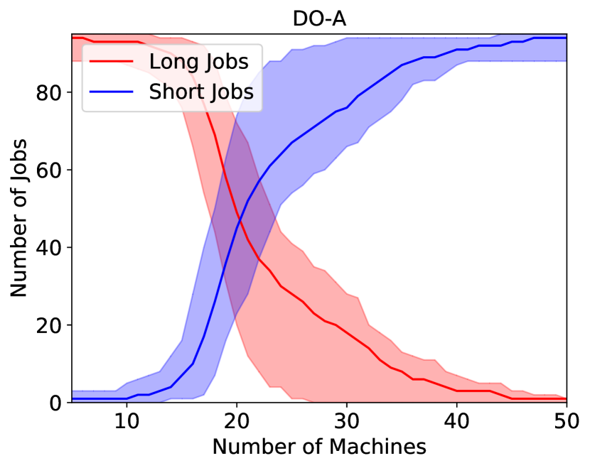
(a) DO-A

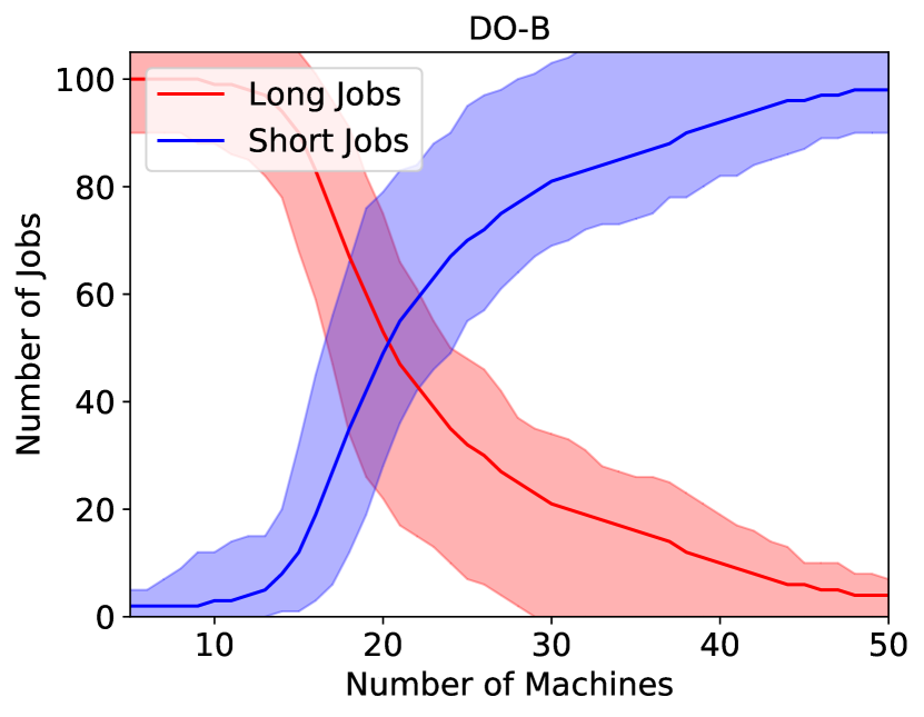
(b) DO-B

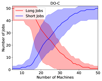
(c) DO-C

Figure 7: Line chart comparing the cardinality of long and short jobs. Given a number $m$ machines, (i) the solid line plots the average cardinality and (ii) the shaded area shows the difference between the maximum and minimum cardinality, with respect to all job sets (days).

This section presents information about the number and processing load of long and short jobs in the instances of each delivery office. Since the long-short job separation depends on the number $m$ of machines, we examine a range of $m$ values. A job set, i.e. the jobs executed by a delivery office in one day, is solved for every $m\in[5,50]$. Let $K$ be the number of examined days for a delivery office, e.g. DO-A. Moreover, denote by $N$ the number of all completed jobs during these $K$ days and by $(P_{1},\ldots,P_{N})$ the corresponding vector of processing times. Then, $N^{L}(m)=|\{j:P_{j}\geq m,1\leq j\leq N\}|$ and $N^{S}(m)=|\{j:P_{j}<m,1\leq j\leq N\}|$ is the total number of long and short jobs, respectively, during all days, assuming $m$ machines. In addition, $\Lambda^{L}(m)=\frac{1}{m}\sum_{j:P_{j}\geq m}P_{j}$ and $\Lambda^{S}(m)=\frac{1}{m}\sum_{j:P_{j}<m}P_{j}$ is the mean load of long and short jobs, respectively, with $m$ machines.

Figure 7 plots the averaged number $\frac{N^{L}(m)}{K}$ and $\frac{N^{S}(m)}{K}$ of long and short jobs per day, with respect to $m$. Similarly, Figure 8 illustrates the averaged mean loads $\frac{\Lambda^{L}(m)}{K}$ and $\frac{\Lambda^{S}(m)}{K}$ per day, with respect to $m$. Clearly, when $m$ increases, $\frac{N^{L}(m)}{K}$ and $\frac{P^{L}(m)}{K}$ decrease, while $\frac{N^{S}(m)}{K}$ and $\frac{P^{S}(m)}{K}$ increase. Section 3 implies that the most difficult instances for LPT arise when the averaged mean load $\frac{\Lambda^{L}(m)}{K}$ of long jobs per day tends to become equal to the averaged number $\frac{N^{S}(m)}{K}$ of short jobs per day. Figures 7-8 show that this pathological situation occurs when $m$ belongs to $[18,25]$, $[20,27]$ and $[23,30]$ for DO-A, DO-B and DO-C, respectively.

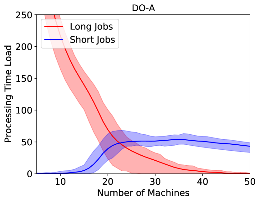
(a) DO-A

(b) DO-B

(c) DO-C

Figure 8: Line chart comparing the processing time load $\frac{1}{m}\sum_{j}p_{j}$ of long and short jobs. Given a number $m$ machines, (i) the solid line plots the average load and (ii) the shaded area shows the difference between the maximum and minimum load, with respect to all job sets (days).

7.3 Evaluation of Heuristics

(a) DO-A

(b) DO-B

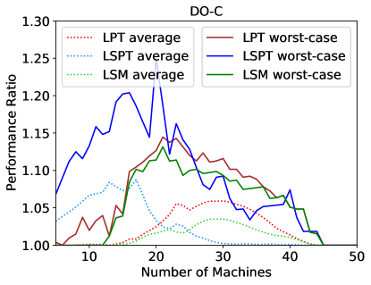
(c) DO-C

Figure 9: Line chart comparing the performance of the heuristics. For a given number $m$ of machines, (i) solid lines plot the worst-case performance ratios and (ii) dotted lines plot the average performance ratios of the heuristics with respect to all jobs sets (days).

This section compares the performance of the LPT (Section 3), LSPT (Section 4) and LSM (Section 5) heuristics for BJSP. For each job set $\mathcal{J}$ (i.e. collection of jobs executed by a delivery office in one day) and number $m\in[5,50]$ of machines, we create a BJSP instance with $g=1$. We solve every instance $I=(m,\mathcal{J})$ using LPT, LSPT and LSM. Let $T(A,I)$ be the makespan of the schedule produced by heuristic $A$ for instance $I$. Then, the performance ratio of heuristic $A$ for $I$ is $T(A,I)/T^{*}(I)$, where $T^{*}(I)$ is the best heuristically computed makespan for $I$.

Figure 9 plots the worst-case and average performance ratio of each heuristic, for each $m$ value. For small $m$ values, the number $n^{S}$ of short jobs is low compared to the mean load $\frac{1}{m}\sum_{j\in\mathcal{J}^{L}}p_{j}$ of long jobs and LPT produces good heuristic schedules, noticeably better than LSPT. As $m$ increases, the idle period before the last job begins becomes progressively more significant and LSPT tends to compute better schedules than LPT (recall that LSPT and LPT achieve low idle machine before and after, respectively, the last job start). Interestingly, LSPT produces the best heuristic schedules in the pathological LPT case where $n^{S}$ tends to become equal to $\frac{1}{m}\sum_{j\in\mathcal{J}^{L}}p_{j}$. Finally, LSM consistently produces better schedules than LPT. Therefore, scheduling short jobs in parallel with long jobs early in a schedule is useful for achieving low makespan. Our findings indicate that a LSM variant where long jobs are executed according to SPT, in parallel with short jobs, might be a possible alternative for obtaining better BJSP approximation algorithms.

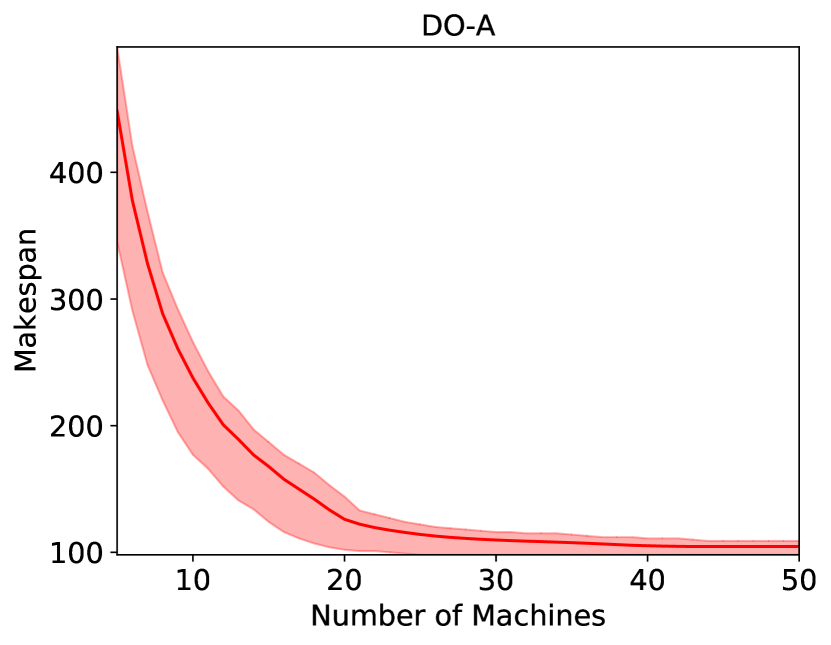
(a) DO-A

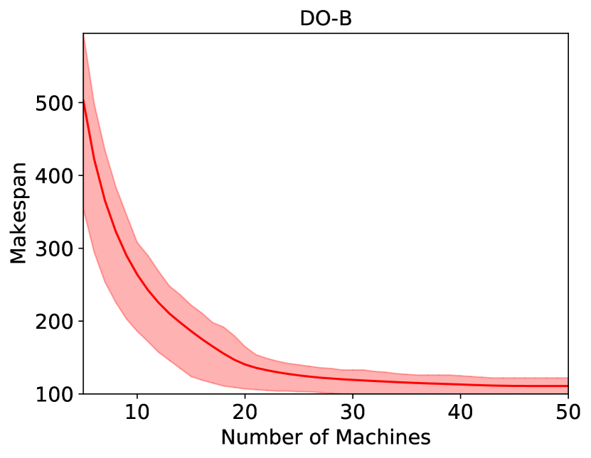
(b) DO-B

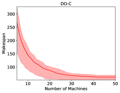
(c) DO-C

Figure 10: Trade-off between the makespan and number of machines. Given a number $m$ machines, (i) the solid line plots the average makespan and (ii) the shaded area shows the difference between the maximum and minimum makespan, with respect to all job sets (days).

For completeness, Figure 10 plots the trade-off between the best heuristically computed makespan $T$ with respect to the number $m$ of machines. Clearly, as $m$ increases, $T$ decreases. This finding supports using machine augmentation for better makespan schedules in the presence of uncertainty.

7.4 Evaluation of Historical Schedules

This section evaluates the Royal Mail historical schedules (i) efficiency in number of used machines and (ii) sensitivity with respect to processing time and (iii) BJSP parameter variations.

For part (i), we solve each BJSP instance by feeding the corresponding MILP (8) model to CPLEX. In these MILP (8) models, we set $\theta=0$ to minimize the number of used machines. Figure 11 compares the number of machines in the Royal Mail historical schedules and the CPLEX solutions. We observe that nominal optimal solutions save at least 10, 25, and 10 vehicles per day compared to historical schedules for DO-A, DO-B, and DO-C, respectively. This finding is a strong indication that more efficient fleet management might be possible in Royal Mail delivery offices.

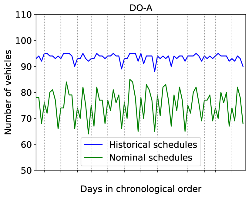
(a) DO-A

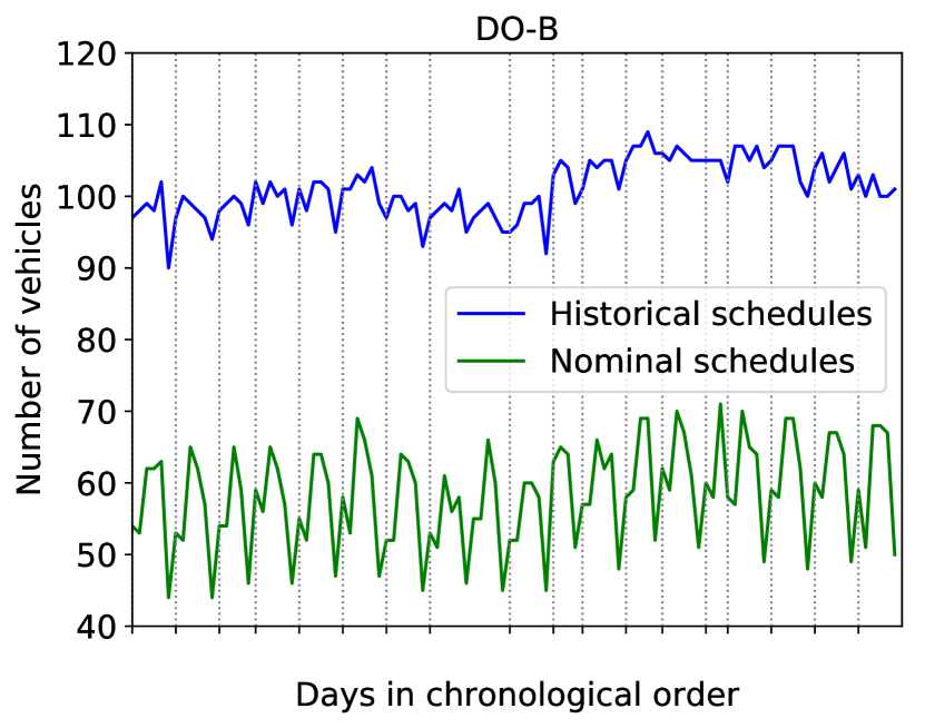
(b) DO-B

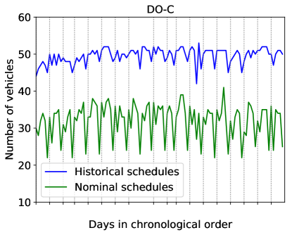
(c) DO-C

Figure 11: Line chart comparing the number of used machines in historical and nominal optimal schedules.

For part (ii), we create a set of perturbed instances. In particular, for each original instance $I$, we create one perturbed instance $\tilde{I}$ where the processing time of each job $j\in\mathcal{J}$ is decreased by a factor $f_{j}=0.5$. We reduce the processing times to guarantee feasibility. For both instances $I$ and $\tilde{I}$, we employ CPLEX to solve the corresponding MILP (8) formulations with $\theta=0$. Figure 12 compares the number of used machines obtained for the original and perturbed instances. Not surprisingly, doubling itinerary durations results in a proportional increase on the number of used vehicles in the nominal optimal solution. But, Figure 12 exhibits an important consequence of uncertainty in Royal Mail fleet management. Disturbances amplify the difference in number of used machines between different days for one delivery office. This situation leads to inefficient machine utilization.

For part (iii), we investigate the effect of modifying the BJSP parameter for each delivery office. Figure 13 depicts the obtained results. Adding BJSP constraints, especially in the DO-B case, may significantly increase the number of used machines. This outcome motivates further investigations on scheduling with BJSP constraints.

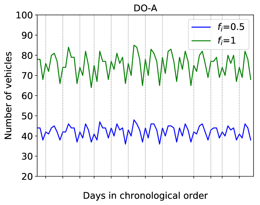
(a) DO-A

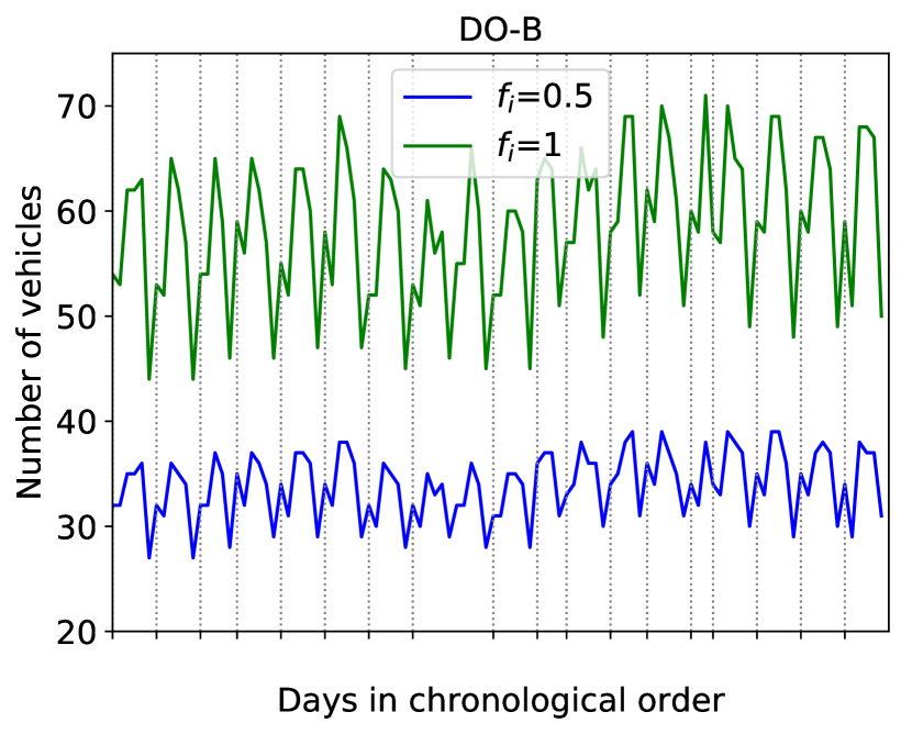
(b) DO-B

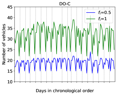
(c) DO-C

Figure 12: Line chart comparing the number of used machines between the original instances and instances where the job processing times have been halved.

(a) DO-A

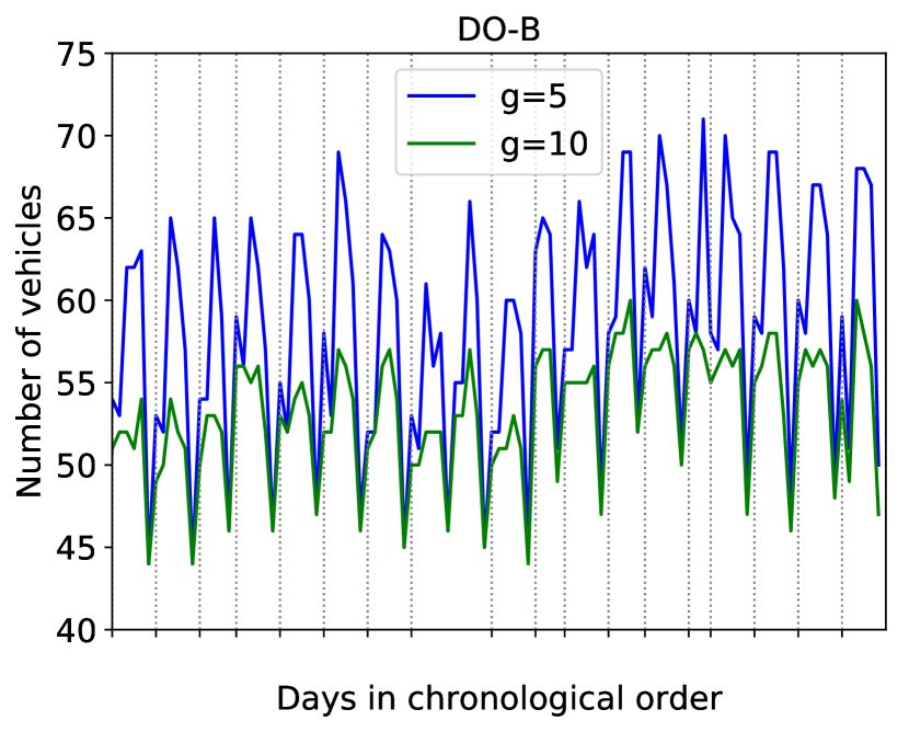
(b) DO-B

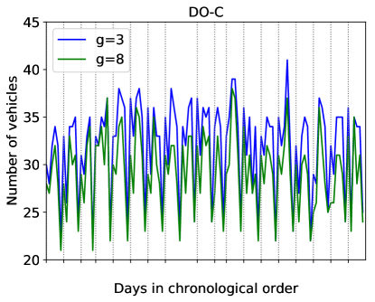
(c) DO-C

Figure 13: Line chart comparing the number of vehicles between instances with different BJSP parameters.

7.5 Robustness Assessment

Next, we evaluate the two-stage robust optimization method in Section 6.2. Specifically, we show that low characteristic value results in more robust BJSP schedules. We adopt the experimental setup in Letsios2018 . The Royal Mail instances are considered as the nominal ones before any disturbances occur. The true instances after uncertainty realization are derived by choosing a new processsing time $\tilde{p}_{j}$ for job each $j\in\mathcal{J}$ uniformly at random from the interval $[p_{j}-50\%p_{j},p_{j}+50\%p_{j}]$, where $p_{j}$ is the nominal processing time.

For each nominal instance $I$, we generate a collection $\mathcal{C}(I)$ of feasible, diverse (i.e. with different characteristic values) first-stage schedules, using the CPLEX solution pool feature. Let $F^{*}(I)=\min\{F(\mathcal{S}):\mathcal{S}\in\mathcal{C}(I)\}$ be the minimum characteristic value among all schedules in $\mathcal{C}(I)$. Next, denote by $\tilde{I}$ and $\tilde{\mathcal{S}}$ the perturbed instance and recovered schedule from $\mathcal{S}$, after uncertainty realization. Moreover, let $V^{*}(\tilde{I})=\min\{V(\tilde{\mathcal{S}}):\mathcal{S}\in\mathcal{C}(I)\}$ be the minimum number of machines achievable for $\tilde{I}$ with perfect knowledge. For each initial schedule $\mathcal{S}\in\mathcal{C}(I)$ and recovered schedule $\tilde{\mathcal{S}}$, we set a normalized characteristic value $F^{N}(\mathcal{S})=F(\mathcal{S})/F^{*}(I)$ and normalized number of used machines $V^{N}(\tilde{\mathcal{S}})=V(\tilde{\mathcal{S}})/V^{*}(\tilde{I})$. Figure 14 correlates $F^{N}(\cdot)$ to $V^{N}(\cdot)$, by plotting every computed pair $(F^{N}(\mathcal{S}),V^{N}(\tilde{\mathcal{S})})$, for every nominal instance and initial solution. We observe that the smaller the initial characteristic value is, the better the final solution we get in terms of number of machines.

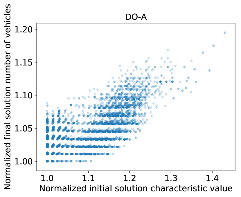
(a) DO-A

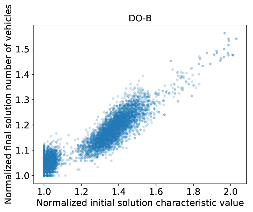
(b) DO-B

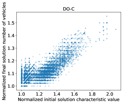
(c) DO-C

Figure 14: Scatter plots comparing the initial solution weighted value with the final solution number of vehicles.

8 Conclusion

This manuscript initiates study of the bounded job start scheduling problem (BJSP), e.g. as arising in Royal Mail deliveries. This project is part of our larger aims towards approximation algorithms for process systems engineering LETSIOS2019106599 . The main contributions are (i) better than 2-approximation algorithms for various cases of the problem and (ii) a two-stage robust optimization approach for BJSP under uncertainty based on machine augmentation and lexicographic optimization, whose performance is substantiated empirically. We conclude with a collection of future directions. Because BJSP relaxes scheduling problems with non-overlapping constraints for which better than 2-approximation algorithms are impossible under widely adopted conjectures, the existence of an algorithm with an approximation ratio strictly better than 2 which does not use resource augmentation is an intriguing open question. A positive answer combining LSM algorithm with a new algorithm specialized to instances with many very long jobs is possible. Moreover, analyzing the price of robustness of the proposed two-stage robust optimization approach may provide new insights for effectively solving BJSP under uncertainty. Our findings demonstrate a strong potential for more efficient Royal Mail resource allocation by using vehicle sharing between different delivery offices. The BJSP scheduling problem where multiple delivery offices are integrated in a unified setting and vehicle exchanges are performed on a daily basis consists a promising direction for fruitful investigations. In this context, recent work on car pooling might be useful. Finally, bounded job start constraints are broadly relevant to vehicle routing problems Fisher1997 ; Gounaris2016 . However, we are not aware of any work in this direction.

- (1) Ben-Tal, A., El Ghaoui, L., Nemirovski, A.: Robust optimization, vol. 28. Princeton University Press (2009)
- (2) Ben-Tal, A., Goryashko, A., Guslitzer, E., Nemirovski, A.: Adjustable robust solutions of uncertain linear programs. Mathematical Programming 99(2), 351–376 (2004)
- (3) Ben-Tal, A., Nemirovski, A.: Robust solutions of linear programming problems contaminated with uncertain data. Mathematical Programming 88(3), 411–424 (2000)
- (4) Bertsimas, D., Brown, D.B., Caramanis, C.: Theory and applications of robust optimization. SIAM review 53(3), 464–501 (2011)
- (5) Bertsimas, D., Caramanis, C.: Finite adaptability in multistage linear optimization. IEEE Transactions on Automatic Control 55(12), 2751–2766 (2010)
- (6) Bertsimas, D., Sim, M.: The price of robustness. Operations Research 52(1), 35–53 (2004)
- (7) Billaut, J.C., Sourd, F.: Single machine scheduling with forbidden start times. 4OR 7(1), 37–50 (2009)
- (8) Chassein, A.B., Dokka, T., Goerigk, M.: Algorithms and uncertainty sets for data-driven robust shortest path problems. European Journal of Operational Research 274(2), 671–686 (2019)
- (9) Davis, R.I., Burns, A.: A survey of hard real-time scheduling for multiprocessor systems. ACM computing surveys (CSUR) 43(4), 35 (2011)
- (10) Fisher, M.L., Jörnsten, K.O., Madsen, O.B.: Vehicle routing with time windows: Two optimization algorithms. Operations research 45(3), 488–492 (1997)
- (11) G, Suraj: A practical analysis of optimisation and recovery under uncertainty. Master’s thesis, Imperial College London (2019). https://www.imperial.ac.uk/media/imperial-college/faculty-of-engineering/computing/public/1819-ug-projects/GS-A-Practical-Analysis-of-Optimisation-and-Recovery-Under-Uncertainty.pdf
- (12) Gabay, M., Rapine, C., Brauner, N.: High-multiplicity scheduling on one machine with forbidden start and completion times. Journal of Scheduling 19(5), 609–616 (2016)
- (13) Garey, M.R., Johnson, D.S.: Computers and intractability, vol. 174. Freeman (1979)
- (14) Goerigk, M., Schöbel, A.: Algorithm engineering in robust optimization. In: L. Kliemann, P. Sanders (eds.) Algorithm Engineering - Selected Results and Surveys, Lecture Notes in Computer Science, vol. 9220, pp. 245–279. Springer (2016)
- (15) Gounaris, C.E., Repoussis, P.P., Tarantilis, C.D., Wiesemann, W., Floudas, C.A.: An adaptive memory programming framework for the robust capacitated vehicle routing problem. Transportation Science 50(4), 1239–1260 (2016)
- (16) Graham, R.L.: Bounds on multiprocessing timing anomalies. SIAM Journal on Applied Mathematics 17(2), 416–429 (1969)
- (17) Hanasusanto, G.A., Kuhn, D., Wiesemann, W.: K-adaptability in two-stage robust binary programming. Operations Research 63(4), 877–891 (2015)
- (18) Kalyanasundaram, B., Pruhs, K.: Speed is as powerful as clairvoyance. Journal of the ACM (JACM) 47(4), 617–643 (2000)
- (19) Kolen, A.W.J., Lenstra, J.K., Papadimitriou, C.H., Spieksma, F.C.R.: Interval scheduling: A survey. Naval Research Logistics 54(5), 530–543 (2007)
- (20) Kouvelis, P., Yu, G.: Robust discrete optimization and its applications, vol. 14. Springer Science & Business Media (2013)
- (21) Letsios, D., Baltean-Lugojan, R., F., Mistry, M., Wiebe, J., Misener, R.: Approximation algorithms for process systems engineering. Computers & Chemical Engineering p. 106599 (2019). DOI https://doi.org/10.1016/j.compchemeng.2019.106599
- (22) Letsios, D., Mistry, M., Misener, R.: Source code (2020). https://github.com/dimletsios/
- (23) Letsios, D., Mistry, M., Misener, R.: Exact lexicographic scheduling and approximate rescheduling. European Journal of Operational Research ((accepted for publication))
- (24) Liebchen, C., Lübbecke, M., Möhring, R., Stiller, S.: The concept of recoverable robustness, linear programming recovery, and railway applications. In: Robust and online large-scale optimization, pp. 1–27. Springer (2009)
- (25) Mnich, M., van Bevern, R.: Parameterized complexity of machine scheduling: 15 open problems. Computers & Operations Research (2018)
- (26) Phillips, C.A., Stein, C., Torng, E., Wein, J.: Optimal time-critical scheduling via resource augmentation. Algorithmica 32(2), 163–200 (2002)
- (27) Rapine, C., Brauner, N.: A polynomial time algorithm for makespan minimization on one machine with forbidden start and completion times. Discrete Optimization 10(4), 241–250 (2013)
- (28) Schäffter, M.W.: Scheduling with forbidden sets. Discrete Applied Mathematics 72(1-2), 155–166 (1997)
- (29) Sherali, H.D.: Equivalent weights for lexicographic multi-objective programs: Characterizations and computations. European Journal of Operational Research 11(4), 367–379 (1982)
- (30) Skutella, M., Verschae, J.: Robust polynomial-time approximation schemes for parallel machine scheduling with job arrivals and departures. Mathematics of Operations Research 41(3), 991–1021 (2016)
- (31) Svensson, O.: Hardness of precedence constrained scheduling on identical machines. SIAM Journal on Computing 40(5), 1258–1274 (2011)
- (32) Xu, H., Mannor, S.: The robustness-performance tradeoff in Markov decision processes. In: B. Schölkopf, J.C. Platt, T. Hoffman (eds.) Advances in Neural Information Processing Systems 19, pp. 1537–1544. MIT Press (2007)