XMP gas-rich dwarfs in Nearby Voids: results of SALT spectroscopy

Abstract

In the framework of an ongoing project aimed at searching for and studying eXtremely Metal-Poor (XMP) very gas-rich blue dwarfs in nearby voids, we conducted spectroscopy with the 11-m Southern African Large Telescope (SALT) of 26 candidates, preselected in the first paper of this series (PEPK19). For 23 of them, we detected Oxygen lines, allowing us to estimate the gas O/H ratio. For ten of them, the oxygen abundance is found to be very low, in the range of 12+$\log$(O/H)=6.95–7.30 dex. Of those, four void dwarfs have 12+$\log$(O/H) $<$ 7.19, or Z $<$ Z_⊙/30. For the majority of observed galaxies, the faint line [Oiii]$\lambda$4363 Å used to estimate O/H with the direct T_e method appeared either too noisy or was not detected. We therefore use the semi-empirical method of Izotov & Thuan (2007) for these spectra, or, when applicable, the new ’Strong line’ method of Izotov et al. (2019b). We present and discuss the results for all void dwarfs observed in this work. We also compare their O/H values with O/H values of $\sim$140 void galaxies available from our recent papers. We address the properties of the newly found unusual void XMP dwarfs and compare them with those for ten known prototype void XMP objects. The latter small group is outstanding based on their very small mass fraction of stars (only 0.01–0.02 of the baryonic mass), the blue colours of stars in the outer body (indicating a non-cosmological age for the main star-forming episode), and the low gas metallicity (several times lower than expected for their luminosity).

1 Introduction

In a recent paper (Pustilnik, Tepliakova & Makarov, 2019, hereafter PTM19) we presented a sample of 1354 Nearby Void Galaxies (the NVG sample), which reside within the boundaries of 25 Nearby Voids, in the volume with distances of $<$ 25 Mpc from the Local Group.

The nearby voids were defined over the entire celestial sphere based on the sample of luminous galaxies defined via the K-band luminosity. They were adopted as those with absolute K-band magnitude $M_{\rm K}<-22.0$. This galaxy sample was used to define empty spheres with minimum radii of 6 Mpc. When the individual empty spheres were close enough, they were joined in groups of spheres. Finally, groups of empty spheres close in space and having common spheres, were also combined into larger entities defined as individual voids with major sizes from $\sim$14 to $\sim$35 Mpc. Of the initial sample of $\sim$7000 objects within the considered volume, 1354 galaxies which appeared inside the found empty spheres, are defined as residing in the abovementioned 25 Nearby Voids. See more details on the Nearby Voids and the galaxies residing in them in PTM19.

One of the goals of selecting this void galaxy sample, was an opportunity to substantially increase the number of unusual void XMP very gas-rich dwarfs from the handful currently known. Most of the known prototype XMP dwarfs were found as a result of the systematic study of a hundred galaxies in the nearby Lynx-Cancer void (Pustilnik, Tepliakova, 2011; Pustilnik et al., 2016, and references therein).

The efficient search for new void XMP dwarfs is based on the preliminary selection of good candidates for the subsequent spectroscopy. The mass selection from the NVG sample is based on the galaxy properties available in public databases and in the literature. This selection is described in the first paper of this series by Pustilnik et al. (2019, MNRAS, accepted, hereafter PEPK19), where a list of 60 selected XMP dwarf void candidates is presented. An overview of the XMP dwarf search and the motivation for the current project are described in detail in the Introduction to that paper. Therefore, we only briefly outline below the main points of the project and the criteria used to select XMP dwarf candidates.

The issue of XMP dwarf galaxies has attracted the attention of astrophysicists since the discovery of the extremely low metallicity of the blue compact dwarf (BCD) IZw18=MRK 116 (Searle & Sargent, 1972), with 12+$\log$(O/H) = 7.17 dex or $Z\sim Z$_⊙/30.

The continuing interest in IZw18, its companion IZw18C, the system SBS0335-052 E,W and similar objects with $Z\lesssim Z$_⊙/30, was motivated by the original idea on their recent first star formation (SF) burst. However, after the discovery of the red giant branch (RGB) population in IZw18, this idea transformed to the less exotic. Namely, such unusual galaxies have probably non-cosmological ages ($\sim$1–2 Gyr) of the main stellar population (Pustilnik, Pramskij, Kniazev, 2004; Izotov et al., 2009; Papaderos, Östlin, 2012; Annibali et al., 2013). Besides, the study of such XMP galaxies is important for understanding star-formation processes at extremely low metallicities typical of galaxies at much earlier epochs.

The term ’very low metallicity’ galaxy was originally applied to objects with gas metallicity below $Z$_⊙/10. Due to the known relation between $Z_{\rm gas}$ and galaxy mass/luminosity (e.g. Kunth & Östlin, 2000) and the many spectroscopic studies of dwarfs in the nearby Universe, metallicities of $Z\lesssim Z$_⊙/10 are now more or less routinely found, so that their current number reaches several hundred (e.g. Guseva et al., 2017).

Table 1: Journal of SALT RSS spectral observations

No.	Name	Date	Expos.	PA	$\theta$″	Air
			time, s			mass
1	PGC000389	2018.10.10	2$\times$1200	26.5	1.5	1.21
2	PGC736507	2018.12.10	2$\times$1200	23.5	1.7	1.29
3	HIJ0021+08$\dagger$	2018.11.07	2$\times$1200	169.0	2.0	1.33
4	AGC104227	2017.11.10	2$\times$1200	121.5	1.5	1.32
5	PGC493444	2017.11.18	2$\times$1200	355.0	1.3	1.30
6	PGC1190331	2018.09.16	6$\times$1200	341.0	1.6	1.19
7	AGC411446	2017.12.08	2$\times$1200	108.0	1.1	1.29
	-#-	2017.12.12	2$\times$1200	108.0	1.8	1.27
	-#-	2017.12.14	2$\times$1200	108.0	1.8	1.27
	-#-	2017.12.15	2$\times$1200	108.0	1.1	1.29
8	AGC114584	2018.10.10	2$\times$1200	157.0	1.5	1.14
	-#-	2018.10.31	2$\times$1200	157.0	1.7	1.14
9	AGC123223	2018.11.09	2$\times$1200	1.0	1.5	1.14
10	AGC124629	2018.11.05	2$\times$1200	310.5	2.0	1.24
	-#-	2018.12.29	2$\times$1200	310.5	2.0	1.24
	-#-	2018.12.30	2$\times$1200	310.5	2.0	1.24
11	AGC132121	2017.11.11	2$\times$1200	320.5	1.3	1.34
12	ESO121-020	2018.11.09	2$\times$1300	142.0	1.3	1.26
	-#-	2019.03.03	2$\times$1300	43.2	1.3	1.26
13	PGC385975	2018.10.10	2$\times$1200	149.0	1.9	1.23
	-#-	2018.11.09	2$\times$1200	142.0	1.3	1.17
14	AGC174605	2018.02.22	2$\times$1200	138.0	1.5	1.32
15	AGC188955	2019.02.27	2$\times$1250	79.0	1.5	1.25
16	AGC198454	2018.12.31	2$\times$1150	202.5	1.1	1.32
17	PGC1314481	2018.02.25	2$\times$1200	172.5	2.5	1.33
18	J1001+0846	2017.12.27	2$\times$1200	303.0	1.3	1.33
19	PGC1230703	2017.12.25	2$\times$1200	22.0	1.6	1.28
20	PGC1178576	2018.02.22	2$\times$1200	137.0	1.5	1.27
21	AGC208397	2019.02.09	2$\times$1300	348.0	1.5	1.28
	-#-	2019.02.27	2$\times$1300	348.0	1.5	1.28
	-#-	2019.02.28	2$\times$1300	348.0	1.5	1.28
	-#-	2019.03.03	2$\times$1300	348.0	1.5	1.28
22	PGC044681	2018.07.06	2$\times$1200	186.5	1.6	1.27
23	PGC135827	2018.02.26	2$\times$1200	324.5	1.5	1.22
24	AGC258574	2018.02.27	2$\times$1200	132.0	1.8	1.27
	-#-	2018.07.08	2$\times$1200	132.0	1.8	1.27
25	KK246	2018.07.04	2$\times$1200	46.0	1.4	1.22
26	AGC335193	2017.11.10	2$\times$1200	227.0	1.8	1.28
$\dagger$ HIJ0021+08 means HIPASSJ0021+08

Our aim is to search for much rarer objects, which we call XMP galaxies, with $Z\lesssim Z$_⊙/30. The main motivation is that in this metallicity range we found several very unusual void dwarfs (see Perepelitsyna et al., 2014; Pustilnik et al., 2016, and references therein). The main advancement in the finding of XMP galaxies is related to the dedicated search for such objects in the enormous spectral database of the SDSS (Abazajian et al., 2009) project (e.g. Guseva et al., 2017; Izotov et al., 2018, 2019a; Sanchez Almeida et al., 2016, and references therein). However, in the whole SDSS DR14 database (Abolfathi et al., 2018) it was possible to identify only about dozen such objects (Izotov et al., 2019b). Together with a handful of XMP dwarfs found by the alternative means (e.g. Searle & Sargent, 1972; Izotov et al., 1990, 2009; Pustilnik, Kniazev, Pramskij, 2005; Pustilnik et al., 2010; Chengalur, Pustilnik, 2013; Skillman et al., 2013; Hirschauer et al., 2016; , Chengalur et al.2016; Hsyu et al., 2017; Takashi et al., 2019), the list of such objects found to date, comprises of only $\sim$20. While a sizable fraction of XMP dwarfs is found outside voids, the majority of such galaxies known to date resides in voids. Besides, for several XMP dwarfs (with Z $<$Z_⊙/30) found via SDSS spectra, the type of environment is not yet published.

Since it was shown that among the least luminous blue dwarfs in voids the fraction of such XMPs can reach $\sim$30% (Perepelitsyna et al., 2014; Pustilnik et al., 2016), we use the NVG sample to produce a list of 60 suitable candidates for further spectral study (PEPK19). The selection was based on the similarity of candidate properties known from public databases and the literature to those of about ten prototype XMP dwarfs (see PEPK19). Those include the elevated gas content, blue colours and low luminosity as well as the indicative strong Oxygen line to H$\beta$ flux ratios, when they were available. See PEPK19 for more detail. In this paper we present the results for 26 of them, available from observations with SALT. The complementary part of the candidate list in the Northern sky was observed at BTA (Big Telescope Alt-azimuth, the SAO 6m telescope) and will appear in an accompanying paper (in preparation).

The rest of this paper is arranged as follows: The description of the SALT spectral observations and data processing is presented in Sec. 2. In Sec. 3 we describe emission line measurements and methods used for O/H determination. In Sec. 4 we show the estimates of O/H for the observed galaxies. In Sec. 5 we discuss the obtained results along with other available information. Finally, in Sec. 6 we present our conclusions. In Appendix A we present plots of 1D spectra for each of the observed galaxies and in Appendix B, tables with line intensities, derived physical parameters and O/H ratios.

2 SALT observations and data processing

Spectral observations with the Southern African Large Telescope (SALT; Buckley, Swart & Meiring, 2006; O’Donoghue et al., 2006) were conducted in service mode in the period from November 2017 to March 2019. Several of the 26 target galaxies were observed from two to four times. See Table 1. We used the SALT Robert Stobie Spectrograph (RSS; Burgh et al., 2003; Kobulnicky et al., 2003) with VPH grating PG0900 with the long slit of 1.5″ by 8′ to cover the range from 3600 Å to 6700 Å  with the resulting spectral resolution of FWHM$\sim$6.0 Å. All spectral data were obtained with a binning factor of four for the spatial scale and factor of two for the spectral coordinate, to give a final spatial sampling of 0$\aas@@fstack{\prime\prime}$51 pixel^-1 and spectral sampling of 0.97 Å pixel^-1 . Since the RSS is equipped with an Atmospheric Dispersion Compensator (ADC), this allowed us to escape the effect of atmospheric dispersion at arbitrary long-slit position angles (PA). Spectrophotometric standards were observed during twilight as part of the SALT standard calibrations program.

SALT is a telescope where the unfilled entrance pupil of the telescope moves during the observations. This implies that the part of the mirror collecting light changes continuously during each specific observation. For that reason absolute flux calibration is not feasible with SALT. However, since all optical elements and instrumentation are always the same, relative flux calibration could be used. Hence, the relative distribution of energy in the spectra could be obtained with SALT data.

Since the majority of Hii-regions in the program galaxies are too faint and low-contrast, we used nearby offset stars for the SALT pointing. Position angles (PAs, in degrees) of the slit (from the North counterclockwise) were selected in most cases to include a nearby offset star and to cover a faint Hii-knot in a program galaxy. See the journal of observation in Table 1 for the main information on each observation including the dates of observations, exposure times, seeing $\theta$ in arc seconds and air mass.

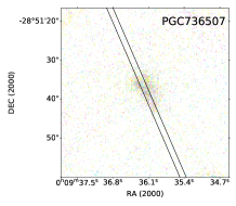
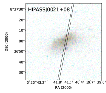
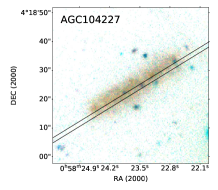
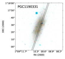
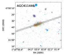
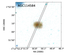
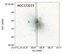
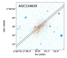
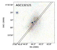
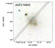
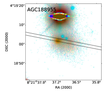
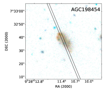
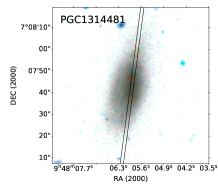
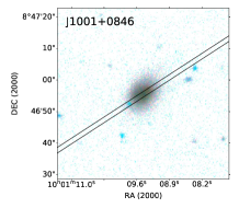
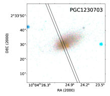
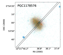
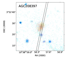
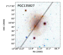
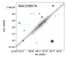
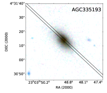
Figure 1: Images of observed galaxies with slit positions superimposed. They are prepared from galaxy images available in the SDSS, PanSTARRS PS1 and DECaLS public databases. Their colours are inverted to better emphasize low surface brightness of the majority observed objects. Galaxy names are printed at the tops of the images. See Table 2 for more details.

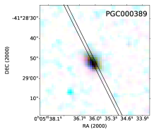
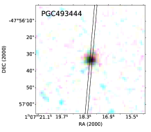
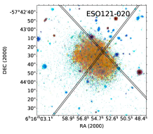
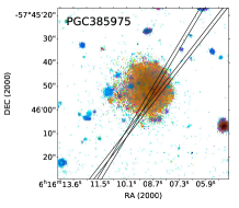
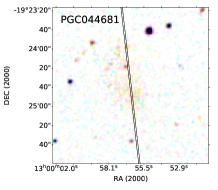
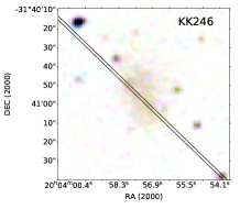
Figure 2: Images of the southern-most observed galaxies with slit positions superimposed. They are prepared from galaxy images available in the ESO DSS (digitized photographic sky surveys based on POSS and SERC) or in DECaLS. Their colours are inverted to better emphasize low surface brightness of the majority observed objects. Galaxy names are printed at the tops of the images. See Table 2 for more details.

As described above, the majority of observed candidate XMP dwarfs are faint and/or of low surface brightness. Therefore an attempt to obtain their independent spectra and to point to the right region can be a problem. To provide an opportunity for independent checks of our data, we present in Table 1 the long slit position angles (PA) and in Figures 1,2 their images with superimposed long slit positions. These images are taken from the SDSS (Abolfathi et al., 2018), PanSTARRS PS1 (Flewelling et al., 2016), DECaLS (Dey et al., 2019) databases and from the ESO Online DSS archive (https://archive.eso.org/dss/dss).

The primary data reduction was done with the SALT science pipeline (Crawford et al., 2010) which includes bias and overscan subtraction and gain correction for each CCD amplifier, cross-talk correction and finally mosaicing. The long-slit reduction, 1D spectra extraction of individual Hii-regions was done in the way described in the recent paper by Kniazev et al. (2018).

3 Line measurements and O/H determination

The emission line fluxes obtained from 1D spectra were measured as described in detail in Kniazev et al. (2004). Here we summarize briefly the main procedures. They include the robust determination of the continuum and its noise level, the subsequent MIDAS-based programs for determination of parameters of emission lines. This uses the procedure of Gauss fitting of emission lines in the continuum-subtracted spectrum. Some lines were fitted as a blend of two or three Gaussians. The quoted errors of line intensities include three components: first – the fitting error from the MIDAS program, related to the Poisson statistics of line photon counts; second – the error resulting from the creation of the underlying continuum; and third – errors related to the accuracy of the sensitivity curve used to transfer counts to relative flux units. The errors of the sensitivity curve are typically no more than (1–2) % so that their contribution to the total error budget is small.

After the line fluxes were measured, we performed an iterative procedure described by Izotov et al. (1994), which accounts for dust extinction and the absorptions in the Balmer lines from the underlying young stellar clusters. This results in the simultaneous estimate of the equivalent width of absorption Balmer lines $EW(abs)$ and the extinction coefficient $C(H\beta)$. The relevant equation (1) from Izotov et al. (1994) was used:

$$I(\lambda)/I(H\beta)=[EW_{e}(\lambda)+EW_{a}(\lambda)]/EW_{e}(\lambda)\times$$

$$EW_{e}(H\beta)/[EW_{e}(H\beta)+EW_{a}(H\beta)]\times$$

$$F(\lambda)/F(H\beta)~{}exp[C(H\beta)f(\lambda)]$$

Here $I(\lambda)$ is the intrinsic line flux corrected for the overall extinction (both in the Milky Way and internal to a particular galaxy) and the underlying Balmer absorption, while $F(\lambda)$ is the measured line flux. $EW_{e}(\lambda)$ are equivalent widths of used emission lines. $EW_{a}(\lambda)$ is the adopted value of the underlying Balmer absorptions. This term is used to estimate intrinsic fluxes only for Balmer emission lines. $f(\lambda)$ is the reddening function adopted from Whitford (1958) and normalized so that $f(H\beta)$ = 0. For the adopted reddening function, there is a relation between the excess E($B-V$) and $C(H\beta)$: E($B-V$) = 0.68 $\times$ $C(H\beta)$.

Due to the low fluxes in the emission lines in the majority of observed Hii-regions, and due to their low metallicities, the principal weak line, [Oiii]$\lambda$4363 Å, used for the determination of the electron temperature T_e in the ’direct’ (T_e) method, was not detected in most of our targets. Therefore, for the estimate of O/H in the majority of the observed galaxies, we used the semi-empirical method suggested by Izotov & Thuan (2007). It was carefully checked and calibrated by the authors and later by us (Pustilnik et al., 2016).

This method uses the fitted empirical dependence between the electron temperature T_e and the value of parameter $R_{\mathrm{2}3}$. This dependence was derived from the analysis of the grid of models of Hii-regions in Stasinska & Izotov (2003). The models approximate well the apparent relations of strong line intensities versus EW(H$\beta$) for the large representative sample of extragalactic Hii-regions, which cover the whole range of observed O/H. Here $R_{\mathrm{2}3}$ is the ratio of the sum of fluxes of strong oxygen lines [Oii]$\lambda$3727 Å, [Oiii]$\lambda$4959 Å, [Oiii]$\lambda$5007 Å to the flux of H$\beta$. When T_e is estimated via $R_{\mathrm{2}3}$, the rest of the calculations uses the standard equations of the classic T_e method. The O/H estimates derived by this method are marked as (se) in Column 9 of Table 2.

For Hii-regions in the lowest metallicity regime, Izotov et al. (2019b) suggested recently an improved empirical method, which uses the relative fluxes of strong Oxygen lines with respect of H$\beta$. Namely, their Equation (1) reads as:

$$12+\log({\rm O/H})=0.950\times\log(R_{\mathrm{2}3}-0.08\times O_{\mathrm{3}2})+6.805$$

Here $O_{\mathrm{3}2}$ is the flux ratio of the line [Oiii]$\lambda$5007 Å to that of [Oii]$\lambda$3727 Å. This relation, calibrated on the large number of Hii-regions with O/H derived via the direct (T_e) method, empirically accounts for the large scatter in the ionization parameter $U$ in various Hii-regions and thus reduces the relatively large internal scatter of other methods based on the strong oxygen lines down to only $\sim$0.05 dex.

However, its applicability is limited only to the range of 12+$\log$(O/H)$\lesssim$7.4. This corresponds to the limit of the combination $R_{\mathrm{2}3}-0.08\times O_{\mathrm{3}2}\lesssim$ 4.0. Since we have among our observed galaxies a dozen objects satisfying this condition, we use this method for them and attach (s) to the derived value of O/H in Column 9 of Table 2, and denote them hereafter as O/H(s).

We notice further that as is evident from the Izotov et al. (2019b) plots in Fig.3b, there is a small offset in the zero-point of O/H(s) relative to that of O/H(T_e), of $\sim$0.03 dex. Therefore, we need to subtract 0.03 dex from O/H(s) ratios to compare them directly with the estimates of O/H(T_e) for other galaxies.

The errors of O/H(s), $\sigma_{\rm log(O/H)}$, due to observational uncertainties in the strong line fluxes are rather small. For our highest signal-to-noise (S/N) spectra, with $\sigma_{\rm R23}$/$R_{\mathrm{2}3}<$0.05, the total error is close to the internal error of the method, $\sigma_{\rm log(O/H)}\sim$0.05 dex. For our lowest S/N spectra, with $\sigma_{\rm R23}$/$R_{\mathrm{2}3}\sim$0.14, the final error of $\log$(O/H)(s) increases to 0.08 dex. For intermediate values of S/N of $R_{\mathrm{2}3}$, the total error is $\sigma_{\rm log(O/H)}$ = 0.06 – 0.07 dex.

Table 2: Observed candidate void XMP dwarfs and new O/H data

No.	Name	J2000 Coord	Vh	D	Bt	$M_{\rm B}$	M(Hi)/	12+$\log$(O/H)	Notes
			km s-1	Mpc	mag	mag	$L_{\rm B}$	$\pm$err.
1	2	3	4	5	6	7	8	9	10
1	PGC000389	J000535.9–412856	1500	17.5	18.23	–13.06	…	7.74$\pm$0.10 (se)
2	PGC736507	J000936.2–285138	7594	104	19.14	–16.00	…	7.58$\pm$0.08 (se)	2dF: wrong Vh=898
3	HIPASSJ0021+08	J002041.7+083655	693	9.9	17.22	–13.34	1.25	7.51$\pm$0.07 (se)
4	AGC104227	J005823.7+041825	1198	16.9	18.12	–13.12	2.11	…	Faint H$\alpha$ at Vh(Hi)
5	PGC493444	J010718.0–475633	7050	95.4	19.22	–15.70	…	…	2dF: wrong Vh=837
6	PGC1190331	J010910.1+011727	1094	15.4	17.54	–13.49	2.24	7.48$\pm$0.08 (se)
7	AGC411446	J011003.7–000036	1137	15.9	19.82	–11.32	6.55	7.05$\pm$0.05 (s)
8	AGC114584	J011250.5+015207	1089	15.4	18.08	–13.02	1.70	7.15$\pm$0.05 (s)
9	AGC123223	J024709.3+100516	767	12.4	18.16	–13.27	2.84	7.47$\pm$0.09 (s)
10	AGC124629	J025605.6+024831	794	12.4	19.46	–11.58	3.61	6.95$\pm$0.06 (s)
11	AGC132121	J030644.1+052008	678	11.0	17.27	–13.68	1.58	7.30$\pm$0.06 (s)
12	ESO121-020	J061554.3–574332	582	6.1	15.73	–13.37	3.30	7.26$\pm$0.05 (s)	aver. 2 knots
13	PGC385975	J061608.5–574551	554	6.1	17.01	–11.91	2.22	7.29$\pm$0.07 (s)	aver. 2 measur.
14	AGC174605	J075021.7+074740	351	9.9	18.68	–11.40	2.90	…	Only H$\alpha$ emission
15	AGC188955	J082137.0+041901	758	12.8	17.70	–12.94	0.85	7.73$\pm$0.08	aver (Te,se). Broad component
16	AGC198454	J092811.3+073237	1373	21.0	18.51	–13.32	1.20	7.52$\pm$0.09 (se)
17	PGC1314481$\dagger$	J094805.9+070743	526	9.2	16.98	–12.96	1.63	7.75$\pm$0.15 (se)
18	J1001+0846	J100109.5+084656	1265	19.2	18.10	–13.56	0.30	7.60$\pm$0.08 (se)
19	PGC1230703	J100425.1+023331	1126	17.1	18.47	–12.80	0.71	7.66$\pm$0.08 (se)
20	PGC1178576	J102138.9+005400	701	11.0	17.27	–13.15	1.30	7.25$\pm$0.06 (s)
21	AGC208397	J103858.1+035227	763	11.9	19.95	–10.59	5.60	7.13$\pm$0.05 (s)
22	PGC044681	J125956.6–192441	827	7.3	17.00	–12.73	3.08	7.20$\pm$0.08 (s)	Faint [Oiii] lines
23	PGC135827	J132812.2+021642	1008	13.5	16.51	–14.25	3.77	7.74$\pm$0.11 (Te)
24	AGC258574	J154507.9+014822	1523	19.3	17.72	–13.09	2.60	7.23$\pm$0.07 (s)
25	KK246	J200357.4–314054	431	7.1	17.07	–13.49	2.33	7.67$\pm$0.08 (se)
26	AGC335193	J230349.0+043113	1125	16.1	17.12	–14.20	0.48	7.57$\pm$0.07 (se)
Table 2 content is described in detail in the third paragraph of Sect. 4. Here we give brief information. Col. 2: target name from NVG.
Col. 3: galaxy coordinates adopted from NVG. Col. 4: radial velocity in km s-1. Columns 5, 6 and 7: the adopted distance,
total blue magnitude and absolute blue magnitude. Col. 8: mass ratio of Hi to blue luminosity, in solar units; Col. 9: derived O/H
as 12+$\log$(O/H) and its error, in dex. In parentheses we indicate the method used: (Te), direct method; (se), semi-empirical
method of Izotov & Thuan (2007), with a small correction from Pustilnik et al. (2016); (s), the new empirical strong line O/H
estimator of Izotov et al. (2019b), with subtracted 0.03 dex to account for a small offset relative to O/H(Te).
In Col. 10 we show brief notes with more detailed information, when necessary, presented in Sec. 5.3.
$\dagger$ in Col 2, O/H(se) based on SALT and SDSS (Abazajian et al., 2009; Abolfathi et al., 2018) spectra.

4 Results of spectral observations and O/H estimates

The 1D SALT spectra of the XMP dwarf candidates are presented in Appendix A, Figs. 4 and 5. The measurements of emission line fluxes as well as derived parameters: the extinction coefficient C(H$\beta$), the adopted equivalent width of Balmer absorption in the underlying stellar continuum EW(abs), and the equivalent width of the H$\beta$ emission line EW(H$\beta$) are presented in Appendix B, Tables B1-B8. For some of the spectra where Balmer absorption was clearly visible in the UV, we modelled the underlying continuum with the ULySS package (http://ulyss.univ-lyon1.fr, Koleva et al., 2009). This model continuum fitted Balmer absorption, and thus corrected to a first approximation the flux of H$\beta$ emission. For these objects, the EW(abs) derived in the next step via iterations as described above with the procedure from Izotov et al. (1994), relates in fact to the residual EW(abs), which is already mainly accounted for by the ULySS fitting. We do not give the absolute flux in the emission H$\beta$ since as explained in Section 2, due to the nature of SALT observations, absolute flux calibration is impossible.

At the bottom of these tables we also give the derived T_e in the zones of emission of [Oiii] and [Oii], the relative numbers of ions O⁺, O⁺⁺ and the total abundance of Oxygen relative to Hydrogen, O/H. Finally, we present for each galaxy the derived parameter 12+$\log$(O/H) obtained with the direct method (for a couple objects where applicable), with the semi-empirical method of Izotov & Thuan (2007) (for all our objects) and with the empirical strong-line method of Izotov et al. (2019b) (for the 10 lowest O/H objects when applicable). We note that 12+$\log$(O/H) derived both with the semi-empirical method and with this new strong-line method are corrected by several 0.01 dex to make zero-points consistent with that for the direct T_e method. See Appendix in Pustilnik et al. (2016) and Sec 3 above for details.

In Table 2 we summarize all adopted O/H estimates along with some other important galaxy parameters. The columns include the following information: Col. 1 – the target number, the same as in Table 1; Col. 2 – the galaxy name as it appears in the NVG catalog, mainly adopted from the HyperLEDA database; Col. 3 – J2000 epoch coordinates; Col. 4 – heliocentric velocity in km s^-1; Col. 5 – Distance in Mpc, either measured with the Tip of the RGB method, or with the use of the peculiar velocity correction according to the velocity field from Tully et al. (2008) as adopted in the Nearby Void Galaxies catalog (PTM19); Col. 6 – an estimate of the total $B$-band magnitude; Col. 7 – the corresponding absolute magnitude $M_{\rm B}$ with the MW extinction correction from Schlafly & Finkbeiner (2011); Col. 8 – the Hi gas-mass to luminosity ratio M(Hi)/$L_{\rm B}$, in solar units; Col. 9 – the parameter 12+$\log$(O/H) with its 1-$\sigma$ uncertainty and the method used (in parentheses); in Col. 10 we provide notes for some of the program galaxies.

Of 26 observed targets, the Oxygen emission lines were detected for 23 galaxies, displaying either Emission-Line type spectra (ELG), or Emission and Absorption line spectra (E+A). However, one of these 23 galaxies appears to be a distant object at $D\sim$ 100 Mpc. One other distant galaxy appeared among the selected XMP void candidates with only absorption lines visible in its spectrum. Both these cases are discussed in more detail in Sect. 5.3. In two more faint LSB dwarfs only H$\alpha$ emission was detected in the SALT spectra. While a more careful check for the possible presence of other Hii-regions can prove useful, the available data indicate a mostly terminated star-formation episode in these two void LSB dwarfs.

For the remaining 22 Nearby Void XMP dwarf candidates, we obtained estimates of O/H with good to acceptable quality. Their derived values of 12+$\log$(O/H) lie in the range of 6.95 to 7.75 dex. Four of them, with 12+$\log$(O/H) in the range of 6.95 – 7.15 dex, appear to be new XMP dwarfs near the edge of the galaxy gas-metallicity distribution, (Z_⊙/50 $\lesssim$ Z $\lesssim$ Z_⊙/30), adding a substantial fraction to about a dozen known galaxies with such a low O/H residing within the nearest cell of the Universe of $R\lesssim 25$ Mpc. For only four of these 22 objects does O/H marginally (that is within the cited uncertainties) exceed the level of (O/H)_⊙/10, corresponding to 12+$\log$(O/H) = 7.69 dex. A more detailed discussion of the presented results follows in Sec. 5

5 Discussion

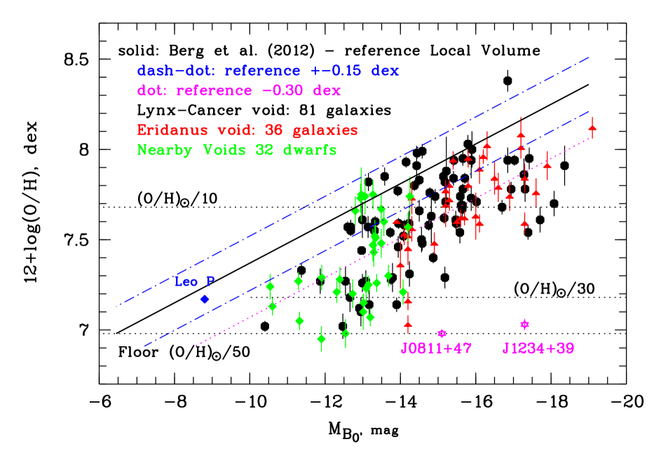
Figure 3: Positions of 22 NVG XMP candidates studied with SALT, plus one known from the literature (J2104–0035) and nine candidates from the BTA part of the program (a paper in preparation), in the diagram 12+$\log$(O/H) versus absolute blue magnitude $M_{\rm B}$ (green rhombs) along with similar data for the Lynx-Cancer (black octagons, Pustilnik et al. 2016) and Eridanus (red triangles, Kniazev et al. 2018) voids. The solid line shows the relation between 12+$\log$(O/H) and $M_{\rm B}$ for the reference sample of the Local Volume late type galaxies from Berg et al. (2012), extrapolated for $M_{\rm B}>$ –10.5. The dotted line running 0.3 dex lower in $\log$(O/H), separates the region in the diagram below –2 $\sigma_{\rm scatter}$ from the reference line. Points in this region are treated as significant outliers. Two outstanding distant record-low metallicity XMP BCGs J0811+4730 and J1234+3901 from the recent papers by Izotov et al. (2018, 2019) are shown by purple stars for comparison. See a more detailed discussion in the text.

As discussed in the previous paper of this series (PEPK19), the prototype void gas-rich XMP dwarfs are atypical compared to other void dwarfs as well as to the general dwarf galaxy population. The four new gas-rich XMP dwarfs of this study residing in Nearby Voids share all the unusual properties of the prototype group. Their O/H is reduced for their $M_{\rm B}$ by a factor of $\sim$2 to $\sim$4 with respect to the reference relation of Berg et al. (2012), or, in other words, their blue luminosity is elevated for their O/H by $\sim$10–100 times with respect to this reference relation. The current SF activity in these XMP dwarfs (with the possible exclusion of AGC114584) is low and does not seem to shift them significantly to the brighter $M_{\rm B}$, which is partly the case for the prototype XMP blue compact galaxy IZw18. As we show in the accompanying paper on these XMP dwarfs’ photometric properties, their mass in stars comprises $\sim$0.01–0.02 of the total baryonic mass. Also, the colours of unresolved stars in their outer parts appear rather blue (as opposed to the majority of the main void galaxy population) and are consistent with ages of one to a few Gyr.

The very atypical properties of XMP dwarfs in the Nearby Voids emphasize the need for advanced model simulations which can reproduce the observed population and, thus, help to understand their formation and specific evolutionary scenarios. One of the ways of confronting the observations and models is related to the Very Young Galaxies (VYGs) defined recently by Tweed et al. (2018) as galaxies that formed most of their stellar mass during the last $\sim$1 Gyr.

In simulations predicting the existence of VYGs (Tweed et al., 2018), neither their gas mass-fraction, nor their type of environment are noticed. The small group of void XMP gas-rich dwarfs, both the prototype galaxies and the four new XMP dwarfs found in this work, due to their observational properties, represent the most natural proxy for the simulated VYGs. At the moment, we do not know whether simulations predict VYGs with less extreme properties. If they do, it seems it will be hard to find them in a systematic manner.

At the same time, very gas-rich XMP dwarfs can be systematically found within the Nearby Voids. Therefore, the use of them as good proxies of simulated VYGs gives the possibility to estimate their lower number fraction. Such an estimate in turn can be helpful for comparison with predictions of VYG number fractions in cosmological models with Cold (CDM) and Warm (WDM) Dark Matter. As Tweed et al. (2018) emphasize, the simulated number of VYGs in WDM cosmology appears many times larger than in the CDM one.

On the other hand, the statistical analysis of already discovered XMP dwarfs and understanding their diversity and the boundaries of their parameter space should help in designing more effective searches for these very rare galaxies.

5.1 General statistics of O/H in void galaxies

To compare our new data on O/H for XMP candidate galaxies from the NVG sample, we plot them in the diagram 12+$\log$(O/H) versus $M_{\rm B}$ (Fig. 3) along with our earlier results for galaxies residing in the Lynx-Cancer (81 filled octagons) (Pustilnik et al., 2016) and Eridanus (36 filled triangles) (Kniazev et al., 2018) voids. To O/H data for 22 NVG dwarfs from this study we added O/H of 9 dwarfs from BTA results (in preparation) and J2104-0035 with O/H from Izotov et al. (2019b). They are shown by green rhombs.

Due to the implied absolute magnitude cut of $M_{\rm B}>-14.3$ for the selected XMP void candidates, our new data occupy the region of the diagram containing about a half of the Lynx-Cancer void sample and $\sim$20% of the Eridanus sample. As one can see, our new O/H data for void galaxies match the results of the previous studies well. Their higher incidence in the range, 12+$\log$(O/H) $\lesssim$7.2, presumably reflects both factors: the $M_{\rm B}$ cut and the additional selection criteria for XMP candidates described in Section 1 and PEPK19.

It is of interest to compare the updated results on void galaxy metallicities with the reference relation 12+$\log$(O/H) versus $M_{\rm B}$ from Berg et al. (2012) derived for the Local Volume galaxies residing in denser environments, mostly in typical groups. Their relation is shown in Fig. 3 by a solid line. Two dash-dot lines show the 1 $\sigma$ scatter of their data points around their linear regression. The dotted line runs 2 $\sigma$ below the reference relation.

As we concluded in Pustilnik et al. (2016), the Lynx-Cancer void sample has as a whole a reduced gas metallicity, with the average O/H deficiency with respect to the reference relation of $\sim$0.18 dex. If we limit the comparison of the reference and void samples with currently available O/H by the cut, $M_{\rm B}>-12.5$, we find that the void sample of a dozen of the lowest luminosity dwarfs has a significantly larger O/H deficiency of $\sim$0.5 dex. This is an interesting finding. However, to date it is difficult to decide whether this is the effect of the special XMP candidate selection or the reflection of stronger environmental effects. To clear up this issue, we need an unbiased measurement of gas metallicity for all available void dwarfs with the lowest luminosities.

The current spectral results were obtained for about a half of the 60 preselected XMP candidates from PEPK19. We expect to find in the remaining part of the original candidate list several other similar objects. The final list of XMP gas-rich void galaxies should be valuable material for a first statistical analysis of such outstanding galaxies. They are interesting by themselves since the combination of their very low stellar mass fraction, non-cosmological ages of the oldest visible stellar population outside regions of current/recent star formation and extremely low gas metallicity indicate their unusual evolutionary status.

In addition, if they can be identified as VYGs, their statistics can provide limits on modern cosmological models as emphasized by Tweed et al. (2018). To this end, apparently more advanced model simulations are necessary that probe a lower mass range of dwarfs, better matching the observed mass range of VYG candidates. It is also important to understand how these nearby XMP dwarfs with low and very low star formation rate (SFR) are connected with the outstanding starbursting XMP dwarfs found by Izotov et al. (2018, 2019a).

The increase in the number of known unusual void dwarfs (with properties summarized in the beginning of Sec. 5) and the advance in the study of their group properties hopefully will provide deeper insights into predicted properties of galaxies with both low baryon mass and tiny fraction of stellar mass.

5.2 New void dwarfs with the lowest metallicities

It is worth describing in more detail the four most extreme XMP dwarfs with $Z\lesssim Z$_⊙/30 (12+$\log$(O/H) $\lesssim$7.2). As seen in Column 9 of Table 2, these are the following dwarfs with the respective values of 12+$\log$(O/H) in parentheses: J0110–0000 (7.05), J0112+0152 (7.15); J0256+0248 (6.95) and J1038+0352 (7.13). All these galaxies are identified as faint Hi-sources in the blind ALFALFA survey (Haynes et al., 2018).

The galaxy, J1259–1924, with the current estimate of O/H of 12+$\log$(O/H)=7.20$\pm$0.08, may also belong to this small group, but its O/H uncertainty is too large and the [Oiii]4959,5007Å lines are extremely faint.

The blue absolute magnitudes M_B of these dwarfs vary between –10.6 and –13.0 (factor of $\sim$9). The respective values of hydrogen mass M(Hi), in the same R.A. order, in units of 10⁷ M_⊙, are as follows: 3.16, 3.92, 1.56, 1.40. That is, the gas mass varies by a factor of $\sim$2.2.

Despite the rather small statistics, it is useful to compare parameters of the new void XMP dwarfs with those for the prototype XMP void group, compiled in Table 1 of PEPK19 paper. The ten prototype XMP dwarfs have a four times broader range of blue luminosities, with M_B between –9.6 and –14.1 (factor of 40). Respectively, their range of M(Hi) (in the same units) is much wider, from 1.6 to 32 (factor of 20). If we combine these 4 new void XMP dwarfs with the prototype XMP dwarfs, they appear to be among the six lowest M(Hi) galaxies of the total of 14 such objects.

While such a situation can occur by chance due to the rather small number statistics of new void XMP dwarfs, this also can hint that our selection procedure introduces some additional bias on the parameter space of XMP dwarfs found in this work. We further address this issue in the abovementioned accompanying paper (in preparation) summarizing the photometric parameters of new XMP dwarfs. It includes data on the stellar masses and their fractions of all examined XMP dwarfs. This also will include additional XMP dwarfs found in the similar program at the SAO 6-m BTA telescope.

5.3 Comments on several individual galaxies

Among the galaxies presented in Table 2 there are several cases which are worth additional comments:

PGC736507 = J0009–2851. This rather distant emission-line galaxy (V_h=7594 km s^-1) appeared in the list of preselected candidates (PEPK19) because an incorrect radial velocity, V_h= 898 km s^-1  appears in 2dFGRS (Colless et al., 2001) and subsequently in HyperLEDA and the NVG sample. Our SALT spectrum of this object shows high-contrast emission lines. Therefore, it is difficult to understand the origin of this error. Moreover, this is not the only case of an incorrect radial velocity among our selected void XMP candidates based on the data of this survey. Based on our experience, we caution potential users on the need for careful checks of 2dFGRS redshifts for objects with radial velocities of $\lesssim$1000 km s^-1.

The gas metallicity of this background dwarf with $M_{\rm B}=-16.0$, corresponding to 12+$\log$(O/H) = 7.58 dex, appears rather low for its luminosity in comparison to the reference relation in Fig. 3. As one can see, its O/H ratio is near the lower limit for dwarfs with the same luminosity residing in the Lynx-Cancer and Eridanus voids. Therefore, it is of interest to examine the nature of its environment.

A check of nearby galaxies in NED within a projected distance of 100′ (3 Mpc at the assumed distance of 104.5 Mpc) reveals the galaxy cluster ABELL 2734 and its probable members at the projected distance of $\sim$0.7 Mpc. The difference in radial velocity between PGC736507 and ABELL 2734 of 201 km s^-1 is not so large as to completely exclude the membership of PGC736507 in ABELL 2734. If this is the case, it is situated at the cluster periphery, at least at the distance of $\sim$0.7 Mpc. In a more probable scenario, where PGC736507 is far from the cluster and the velocity difference is due to the Hubble flow (with adopted H${}_{\mathrm{0}}=73$ km s^-1 Mpc^-1), it is at $\sim$2.8 Mpc from the nearest luminous/massive galaxy, that is, in a rather low-density environment. The latter case would be more consistent with its low observed metallicity.

We noticed a faint bluish nebulosity (J0009–2852) at $\sim$50″ SSW of the target galaxy, which could be its companion. Therefore, the slit was positioned across this potential companion. As its spectrum revealed (see Fig. 4), it appears to be a distant ELG with the redshift $z=$ 0.20159. The strong line ratios in the spectrum are typical of star-forming galaxies. We estimate its 12+$\log$(O/H) $\sim 8.2\pm$0.1 dex using the lower branch of the strong line empirical estimator of Pilyugin, Thuan (2005).

PGC493444 = J0107–4756. This rather distant absorption-line galaxy has radial velocity V_h=7050 km s^-1, as revealed by several Balmer lines in its spectrum. It appeared in the list of preselected void XMP candidates (PEPK19) also due to a mistaken radial velocity V_h = 837 km s^-1 in 2dFGRS (Colless et al., 2001) and then, in HyperLEDA and the NVG sample.

ESO121-020 = J0615–5743. The slit for this spectrum passed through two nebulous emission knots and a star-like emission object in between (as revealed by our H$\alpha$ image obtained with SALT before the spectral observation). The very low values of O/H in both nebulosities are the same within the cited errors. Therefore, we adopt for this galaxy the average of the two Hii-regions.

The star-like object displays Balmer absorptions in the UV and H$\alpha$ and H$\beta$ in emission, but no hint of nebular emission lines. Moreover, H$\alpha$ has broad underlying wings with a FWHM of $\sim$ 800 km s^-1. The estimate of its $B$ magnitude, $\sim 22.5$, implies an absolute magnitude $M_{\rm B}\sim-6.5$, characteristic of supergiants. Having only this rather low S/N spectrum, it is difficult to make more or less reasonable suggestions on the nature of this object. However, one of the options is a composite spectrum of a young stellar cluster with an age of 12–13 Myr estimated from the EW of the narrow component, EW(H$\alpha$) = 31 Å  (according to Leitherer et al. (1999)), and a luminous emission-line star of a comparable luminosity. It could be an LBV in a relatively faint phase. A more advanced characterization of this emission star-like object requires more data on possible variability and other emission lines.

PGC385975 = J0616–5745. For this companion of ESO121-020, we obtained two independent spectra of two different Hii-regions. Their O/H values are consistent with each other within their errors, so we adopt their mean value.

AGC188955 = J0821+0419. There are two emission-line knots in the 2D spectrum. In the brighter knot all suitable lines are well measured and its O/H is derived with the direct method (see Table B4). In the fainter knot the [Oiii]$\lambda$4363 Å line is undetected and its O/H is estimated via the method of Izotov & Thuan (2007). The 12+$\log$(O/H) values differ for the two knots: 7.81$\pm$0.08 for the brighter and 7.64$\pm$0.08 for the fainter. However, since the difference is only $\sim$1.5 $\sigma$ of the combined error of O/H, we adopt for this galaxy the average O/H of the two knots. The brighter knot displays a low-contrast broad (FWHM $\sim$ 1050 km s^-1) underlying component in the strong lines, best visible in H$\alpha$ and [Oiii]$\lambda$5007 Å. For the O/H estimate the flux in the broad component was not included. In the [Oiii]$\lambda$5007 Å line, the flux of the broad component comprises $\sim$0.07 of the narrow component. The nature of this broad component is unclear. However, in low-metallicity galaxies with active star formation the appearance of broad components of strong emission lines is not rare (e.g. Izotov, Thuan, Guseva, 2007). If this phenomenon is not related to the short phase of WR stars, then the collective effect of many SNR and the related fast shells could make the main contribution to the observed broad components.

PGC1314481 = J0948+0707. Our SALT spectrum is rather noisy and certainly of worse quality in comparison to the spectrum of this object presented in the SDSS spectral database. For an optimal estimate of O/H in this galaxy, we use its spectral data from SDSS and add the flux of [Oii]$\lambda$3727 Å from our SALT spectrum. To combine this line flux correctly with fluxes of other lines in the SDSS spectrum, we carefully checked the similarity of the relative fluxes of the strongest Balmer and [Oiii] lines in the SDSS and SALT spectra.

KK246 = J2003–3104 = ESO461-036 = SIGRID68. This Local Volume gas-rich galaxy, with a Milky Way (MW) $B$-band extinction of $A_{\rm B}=1.10$ (Schlafly & Finkbeiner, 2011), has been studied many times, including by Kreckel et al. (2011) and by Nicholls et al. (2014). Its O/H was first derived by Nicholls et al. (2014) with a spectrum without detected [Oiii]$\lambda$4363 Å. Using their Mapping IV model analysis (Dopita et al., 2013), these authors derive 12+$\log$(O/H)$\sim$8.2 dex. That is, our (7.67$\pm$0.08 dex) and their O/H determinations differ significantly and need further examination. The first factor of the difference, which Nicholls et al. (2014) emphasize, is due to the known systematics of $\sim$0.2 dex between the two methods. However, there still remains an additional difference of $\sim$0.3 dex.

It appears that there are problems with the primary uncorrected spectrum of this object obtained with the WiFeS IFU spectrograph at the ANU 2.3-m telescope. Their observed Balmer decrement implies an overall extinction A_V of only 0.032 mag for KK246, equivalent to A${}_{\rm B}=0.042$. At the same time, as mentioned above, the known MW extinction in this direction is much higher, $A_{\rm B}=1.10$.

The Balmer decrement of our uncorrected spectrum implies C(H$\beta$) = 0.60$\pm$0.05. This translates, for the standard extinction curve, to $A_{\rm B}=1.75$$\pm$0.15, which does not contradict the minimal expected value of $A_{\rm B}=1.10$. In terms of C(H$\beta$), the MW $A_{\rm B}=1.10$ implies a minimum expected C(H$\beta$)=0.38. Our measured C(H$\beta$) = 0.60$\pm$0.05, after subtraction of the MW contribution, implies an internal C(H$\beta$,inter) = 0.22$\pm$0.05 dex, which is quite typical of low-metallicity dwarfs (e.g. Guseva et al., 2017, and references therein).

Another doubtful issue with the data of Nicholls et al. (2014) is the extremely low level of the underlying continuum in their original spectrum. In our long-slit spectrum the underlying continuum is basically visible. The related EW(H$\beta$) = 29 Å. This brief examination of the two results indicates that our O/H estimate for KK246 should be treated as closer to reality. With our O/H = (O/H)_⊙/10, KK246 in the diagram 12+$\log$(O/H) vs M_B in Fig. 3 sits well within the main cloud of void dwarfs in contrast to the result of Nicholls et al. (2014) (their Fig. 12).

6 Conclusions

In the previous paper (PEPK19) we selected 60 candidate XMP void objects from the fainter part ($M_{\rm B}\gtrsim-14.3$) of the Nearby Void Galaxies (NVG) sample. They were selected based on the similarity of their properties (available in public databases and in the literature) to those of ten known XMP very gas-rich void dwarfs. Here we present the first results of spectral observations of these candidates with SALT.

Summarizing the results presented here and the related discussion, we draw the following conclusions:

1. To date, 26 of the void XMP candidates have been observed with SALT. For 23 of them, Oxygen lines were detected along with Balmer lines and estimates of their gas O/H were derived. They appear in the range of 12+$\log$(O/H) between $\sim$6.95 and $\sim$7.8 dex, with the exception of one emission line galaxy which appeared to be a background object. The majority of our void galaxies with measured O/H fall in the 12+$\log$(O/H) vs M_B diagram within the O/H range typical of void galaxies for their luminosity. Of the 22 Nearby Void galaxies in this study, ten have the parameter 12+$\log$(O/H)$<$7.39 dex, or Z_gas below Z_⊙/20. Such galaxies are still quite rare and their addition will improve their statistics and seemingly increase the diversity of their properties.

2. Of these ten objects, four XMP dwarfs have 12+$\log$(O/H) $<$7.19 dex, or $Z<Z$_⊙/30. One of them, AGC124629=J0256+0248, shows one of the lowest gas-metallicities in the Local Universe (12+$\log$(O/H)=6.95$\pm$0.06) and is the first LSB dwarf with that record-low Z_gas found. Looking ahead, based on an accompanying paper on their photometric parameters (in preparation) and the discussion in Sec. 5, these new XMP dwarfs have unusual properties: blue colours of the outer parts, corresponding to non-cosmological ages of the oldest visible stellar population, and extremely large gas-mass fraction, $\sim$0.98–0.99. Thus, they appear to be very similar to those of the original small XMP group in the Lynx-Cancer and other nearby voids. These four new XMP void dwarfs add to the group of eight nearby prototype XMP void dwarfs (those with known O/H from Table 1 of PEPK19). Thus, the number of void candidate Very Young Galaxies has grown to a dozen. This also allows us to better study their similarity and diversity as well as their finer properties related to their origin and evolution.

3. The results of SALT spectroscopy of the selected XMP candidate list in the NVG sample gives a reasonably high detection rate for the objects that we are primarily looking for and qualifies the search method as an efficient one. This could also be a feasible method to use for an XMP dwarf search in the farther parts of the Local Supercluster.

Appendix A 1D spectra

In this Appendix we present plots of the 1D SALT spectra of the XMP candidates discussed in this paper. The wavelengths on the $X$ axis are observed, not in the rest-frame. For the candidate galaxy PGC736507, we also obtained on the slit the spectrum of a nearby bluish galaxy J0009–2852 (see comments in Sec. 5.3). We present it in Fig. 4 along with a spectrum of PGC736507.

For the program galaxy, ESO121-020, we give two spectra: the first one of an Hii-region, the second of a star-like object with only H$\alpha$ and H$\beta$ in emission (see Sec. 5.3 for details).

For the galaxy, AGC188955, we obtained quite different spectra for two knots which we also discuss in Section 5.3. We show both of them in Fig. 5.

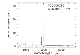
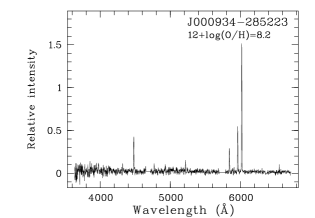
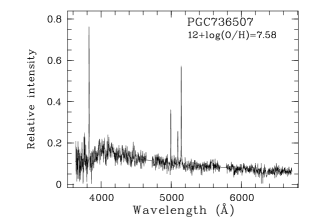
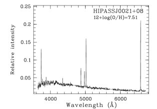
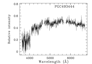
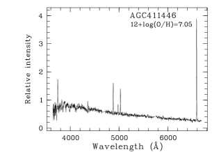
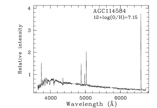
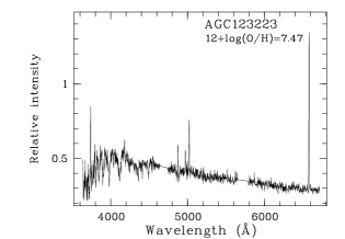
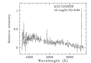
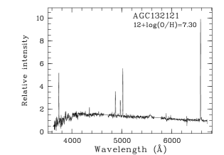
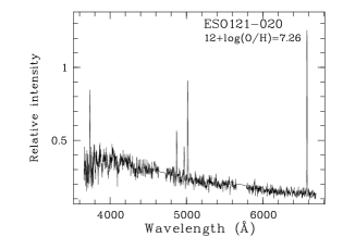
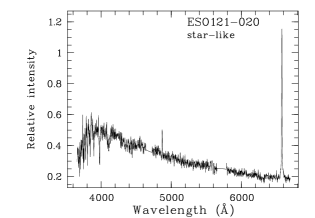
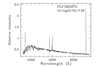
Figure 4: 1D spectra of void XMP candidates obtained with SALT. The wavelengths are not in the rest-frame. The galaxy name and derived value of 12+$\log$(O/H) are shown at the top of each box. See the text for discussion of individual objects.

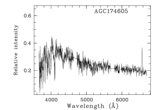
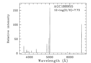
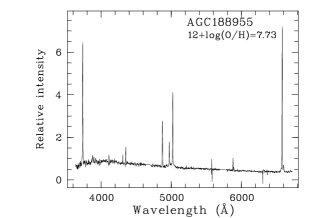
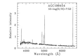
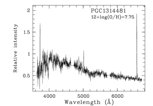
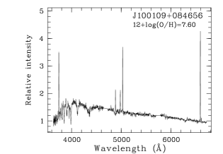
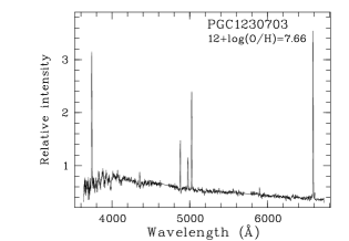
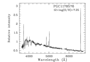
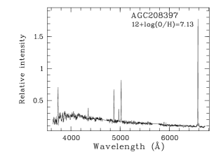
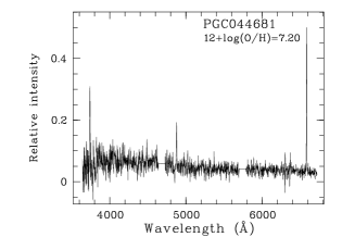
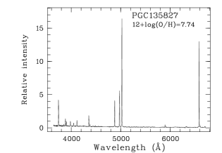
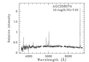
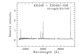
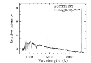
Figure 5: 1D spectra of void XMP candidates obtained with SALT. The wavelengths are not in the rest-frame. The galaxy name and derived value of 12+$\log$(O/H) are shown at the top of each box. See the text for discussion of individual objects.

Appendix B Tables with line fluxes and derived parameters

The tables in this Appendix include the measured line fluxes $F(\lambda)$ (divided by the flux of H$\beta$) and the line fluxes $I(\lambda)$, corrected for extinction and underlying stellar Balmer absorption, with their errors. The error for $F(H\beta)$ reflects its measurement uncertainty. The tables also include the measured $EW$ of H$\beta$ emission and the derived parameters: the extinction coefficient $C(H\beta)$, the equivalent width of the underlying stellar Balmer absorptions $EW(abs)$, the electron temperatures T_e(OIII) and T_e(OII) in two zones of Oxygen ionization. We also present the derived Oxygen abundances in two stages of ionization and the total value of O/H, including its value in units of 12+$\log$(O/H). Electron densities $n_{\rm e}$ in Hii-regions could not be estimated because the doublet [Sii]$\lambda\lambda$6716,6730 Å was outside the observed wavelength range. In this case we adopted $n_{\rm e}$ to be 10 per cm³, typical of Hii-regions in dIrr galaxies.

When the faint auroral line [Oiii]$\lambda$4363 Å was found in the spectra, O/H was estimated via the direct method and marked as 12+$\log$(O/H)(T_e). Otherwise we used two methods described in Sec. 3. O/H values derived via the semi-empirical method of Izotov & Thuan (2007) are marked as (se) with subscript (c), which means the small correction to the original value of O/H derived with the method. The correction of 0.0-0.05 dex was derived in Pustilnik et al. (2016) to put estimates of O/H(se) onto the zero-point of the direct method. For the lowest O/H objects, we employed the new empirical method by Izotov et al. (2019b) based on the relative fluxes of strong Oxygen lines. The values of O/H estimated by this method are marked (s). The subscript (c) for these estimates also means a small correction (–0.03 dex) was applied to the original method value, which puts them on the zero-point of the direct method.

We do not include the following objects from Table 2 in Tables B1-B8 with emission line data: a) PGC736507 and PGC493444 because they are not included in the NVG sample and are interlopers due to an incorrect radial velocity in the original 2dFGRS catalog; b) AGC104227 and AGC174605 – since they show only faint H$\alpha$ emission in the spectra.

For the galaxy, AGC188955 (J0821+0419), for two knots we have very different line ratios but rather similar O/H ratios. Therefore we include data for both knots.

Table 3: Line intensities and derived parameters of PGC000389, HIPASSJ0021+08 and PGC1190331

	PGC000389=J0005–4128		HIPASSJ0021+08		PGC1190331=J0109+0117
$\lambda_{0}$(Å) Ion	$F(\lambda)/F(H\beta)$	$I(\lambda)/I(H\beta)$	$F(\lambda)/F(H\beta)$	$I(\lambda)/I(H\beta)$	$F(\lambda)/F(H\beta)$	$I(\lambda)/I(H\beta)$
3727 [O ii]	0.973$\pm$ 0.021	0.944$\pm$ 0.027	2.026$\pm$ 0.075	1.836$\pm$ 0.085	1.889$\pm$ 0.048	1.849$\pm$ 0.054
3967 [Ne iii] + H7	0.166$\pm$ 0.010	0.199$\pm$ 0.015	…	…	…	…
4101 H$\delta$	0.197$\pm$ 0.007	0.228$\pm$ 0.011	…	…	0.145$\pm$ 0.016	0.168$\pm$ 0.023
4340 H$\gamma$	0.356$\pm$ 0.019	0.378$\pm$ 0.022	0.342$\pm$ 0.028	0.475$\pm$ 0.094	0.319$\pm$ 0.030	0.335$\pm$ 0.035
4861 H$\beta$	1.000$\pm$ 0.025	1.000$\pm$ 0.026	1.000$\pm$ 0.037	1.000$\pm$ 0.077	1.000$\pm$ 0.028	1.000$\pm$ 0.030
4959 [O iii]	1.477$\pm$ 0.036	1.434$\pm$ 0.036	0.816$\pm$ 0.034	0.701$\pm$ 0.034	0.627$\pm$ 0.020	0.614$\pm$ 0.020
5007 [O iii]	4.436$\pm$ 0.096	4.307$\pm$ 0.097	2.421$\pm$ 0.069	2.076$\pm$ 0.069	1.917$\pm$ 0.047	1.876$\pm$ 0.047
6548 [N ii]	0.014$\pm$ 0.011	0.014$\pm$ 0.011	0.008$\pm$ 0.007	0.007$\pm$ 0.007	0.035$\pm$ 0.021	0.034$\pm$ 0.021
6563 H$\alpha$	2.857$\pm$ 0.120	2.793$\pm$ 0.131	3.289$\pm$ 0.117	2.767$\pm$ 0.129	2.806$\pm$ 0.091	2.761$\pm$ 0.100
6584 [N ii]	0.043$\pm$ 0.029	0.042$\pm$ 0.029	0.026$\pm$ 0.026	0.021$\pm$ 0.025	0.110$\pm$ 0.029	0.107$\pm$ 0.029
$C(H\beta)$ dex	0.00$\pm$0.05		0.07$\pm$0.05		0.00$\pm$0.04
$EW(abs)$ Å	1.85$\pm$0.28		2.30$\pm$0.92		0.55$\pm$0.26
$EW(H\beta)$ Å	62$\pm$ 1		14$\pm$ 1		25$\pm$ 1
$T_{\rm e}$(OIII)(K)	14966$\pm$1010		17171$\pm$1029		17536$\pm$1014
$T_{\rm e}$(OII)(K)	13888$\pm$517		14720$\pm$250		14801$\pm$201
O+/H+($\times$105)	1.095$\pm$0.138		1.765$\pm$0.124		1.747$\pm$0.090
O++/H+($\times$105)	4.760$\pm$0.815		1.656$\pm$0.231		1.415$\pm$0.186
O/H($\times$105)	5.855$\pm$0.827		3.421$\pm$0.262		3.162$\pm$0.207
12+log(O/H)c(se)	7.74$\pm$0.10		7.51$\pm$0.07		7.48$\pm$0.08

Table 4: Line intensities and derived parameters of AGC411446, AGC114584 and AGC123223

	AGC411446=J0110–0000		AGC114584=J0112+0152		AGC123223=J0247+1005
$\lambda_{0}$(Å) Ion	$F(\lambda)/F(H\beta)$	$I(\lambda)/I(H\beta)$	$F(\lambda)/F(H\beta)$	$I(\lambda)/I(H\beta)$	$F(\lambda)/F(H\beta)$	$I(\lambda)/I(H\beta)$
3727 [O ii]	1.105$\pm$ 0.057	1.067$\pm$ 0.064	1.232$\pm$ 0.052	0.951$\pm$ 0.056	2.154$\pm$ 0.232	2.295$\pm$ 0.340
3967 [Ne iii] + H7	0.027$\pm$ 0.005	0.197$\pm$ 0.062	…	…	…	…
4101 H$\delta$	0.098$\pm$ 0.010	0.271$\pm$ 0.037	…	…	…	…
4340 H$\gamma$	0.346$\pm$ 0.035	0.480$\pm$ 0.058	0.283$\pm$ 0.022	0.478$\pm$ 0.057	0.231$\pm$ 0.058	0.487$\pm$ 0.185
4861 H$\beta$	1.000$\pm$ 0.024	1.000$\pm$ 0.028	1.000$\pm$ 0.030	1.000$\pm$ 0.041	1.000$\pm$ 0.089	1.000$\pm$ 0.121
4959 [O iii]	0.276$\pm$ 0.025	0.239$\pm$ 0.025	0.544$\pm$ 0.022	0.418$\pm$ 0.022	0.643$\pm$ 0.093	0.479$\pm$ 0.092
5007 [O iii]	0.822$\pm$ 0.026	0.711$\pm$ 0.026	1.591$\pm$ 0.043	1.223$\pm$ 0.043	1.769$\pm$ 0.144	1.303$\pm$ 0.140
6548 [N ii]	…	…	0.015$\pm$ 0.043	0.011$\pm$ 0.043	0.042$\pm$ 0.119	0.022$\pm$ 0.084
6563 H$\alpha$	3.368$\pm$ 0.082	2.715$\pm$ 0.082	3.372$\pm$ 0.144	2.729$\pm$ 0.165	4.965$\pm$ 0.380	2.770$\pm$ 0.304
6584 [N ii]	…	…	0.047$\pm$ 0.056	0.036$\pm$ 0.056	0.147$\pm$ 0.140	0.078$\pm$ 0.098
$C(H\beta)$ dex	0.14$\pm$0.03		0.01$\pm$0.06		0.47$\pm$0.10
$EW(abs)$ Å	2.65$\pm$0.05		3.80$\pm$0.18		1.20$\pm$0.08
$EW(H\beta)$ Å	18$\pm$ 1		13$\pm$ 1		4$\pm$ 1
$T_{\rm e}$(OIII)(K)	22089$\pm$1056		20596$\pm$1038		17904$\pm$1302
$T_{\rm e}$(OII)(K)	16222$\pm$229		15636$\pm$14		14866$\pm$200
O+/H+($\times$105)	0.765$\pm$0.056		0.760$\pm$0.045		2.140$\pm$0.330
O++/H+($\times$105)	0.334$\pm$0.033		0.663$\pm$0.070		0.967$\pm$0.180
O/H($\times$105)	1.099$\pm$0.065		1.422$\pm$0.083		3.107$\pm$0.376
12+log(O/H)c(se)	7.04$\pm$0.08		7.15$\pm$0.08		7.47$\pm$0.09
12+log(O/H)c(s)	7.05$\pm$0.05		7.15$\pm$0.05		…

Table 5: Line intensities and derived parameters of AGC124629, AGC132121 and ESO121-020

	AGC124629=J0256+0248		AGC132121=J0306+0520		ESO121-020=J0615–5743
$\lambda_{0}$(Å) Ion	$F(\lambda)/F(H\beta)$	$I(\lambda)/I(H\beta)$	$F(\lambda)/F(H\beta)$	$I(\lambda)/I(H\beta)$	$F(\lambda)/F(H\beta)$	$I(\lambda)/I(H\beta)$
3727 [O ii]	0.972$\pm$ 0.119	0.976$\pm$ 0.123	2.207$\pm$ 0.117	1.673$\pm$ 0.128	2.479$\pm$ 0.302	1.663$\pm$ 0.318
4340 H$\gamma$	…	…	0.282$\pm$ 0.025	0.477$\pm$ 0.067	…	…
4861 H$\beta$	1.000$\pm$ 0.039	1.000$\pm$ 0.047	1.000$\pm$ 0.046	1.000$\pm$ 0.067	1.000$\pm$ 0.105	1.000$\pm$ 0.184
4959 [O iii]	0.157$\pm$ 0.042	0.153$\pm$ 0.042	0.684$\pm$ 0.037	0.501$\pm$ 0.037	0.703$\pm$ 0.084	0.469$\pm$ 0.084
5007 [O iii]	0.463$\pm$ 0.044	0.450$\pm$ 0.043	2.037$\pm$ 0.079	1.490$\pm$ 0.079	1.818$\pm$ 0.159	1.214$\pm$ 0.159
6548 [N ii]	…	…	0.023$\pm$ 0.048	0.016$\pm$ 0.046	0.017$\pm$ 0.116	0.011$\pm$ 0.115
6563 H$\alpha$	2.847$\pm$ 0.097	2.701$\pm$ 0.102	3.616$\pm$ 0.164	2.750$\pm$ 0.185	3.793$\pm$ 0.355	2.762$\pm$ 0.424
6584 [N ii]	…	…	0.072$\pm$ 0.058	0.051$\pm$ 0.056	0.083$\pm$ 0.149	0.055$\pm$ 0.148
$C(H\beta)$ dex	0.04$\pm$0.04		0.04$\pm$0.06		0.01$\pm$0.12
$EW(abs)$ Å	0.60$\pm$0.57		3.95$\pm$0.22		2.20$\pm$0.39
$EW(H\beta)$ Å	24$\pm$ 1		11$\pm$ 1		4$\pm$ 1
$T_{\rm e}$(OIII)(K)	23542$\pm$1271		18538$\pm$1076		19079$\pm$1412
$T_{\rm e}$(OII)(K)	16499$\pm$208		14939$\pm$82		14962$\pm$15
O+/H+($\times$105)	0.666$\pm$0.087		1.536$\pm$0.120		1.519$\pm$0.291
O++/H+($\times$105)	0.188$\pm$0.027		1.002$\pm$0.133		0.796$\pm$0.151
O/H($\times$105)	0.854$\pm$0.091		2.538$\pm$0.179		2.315$\pm$0.328
12+log(O/H)c(se)	6.93$\pm$0.09		7.39$\pm$0.07		7.35$\pm$0.09
12+log(O/H)c(s)	6.95$\pm$0.06		7.30$\pm$0.06		7.26$\pm$0.07

Table 6: Line intensities and derived parameters of PGC385975 and AGC188955=J0821+0419

	PGC385975=J0616–5745		AGC188955–bright component		AGC188955–faint component
$\lambda_{0}$(Å) Ion	$F(\lambda)/F(H\beta)$	$I(\lambda)/I(H\beta)$	$F(\lambda)/F(H\beta)$	$I(\lambda)/I(H\beta)$	$F(\lambda)/F(H\beta)$	$I(\lambda)/I(H\beta)$
3727 [O ii]	2.121$\pm$ 0.282	2.353$\pm$ 0.389	0.899$\pm$0.014	0.923$\pm$0.017	2.959$\pm$0.068	2.912$\pm$0.076
3868 [Ne iii]	…	…	0.331$\pm$0.008	0.336$\pm$0.009	0.222$\pm$0.041	0.218$\pm$0.041
3889 [He i] + H8	…	…	0.162$\pm$0.016	0.241$\pm$0.028	…	…
3967 [Ne iii] + H7	…	…	0.230$\pm$0.005	0.304$\pm$0.008	…	…
4101 H$\delta$	0.092$\pm$ 0.026	0.265$\pm$ 0.098	0.219$\pm$0.004	0.293$\pm$0.007	0.161$\pm$0.011	0.178$\pm$0.016
4340 H$\gamma$	0.338$\pm$ 0.050	0.481$\pm$ 0.084	0.402$\pm$0.011	0.457$\pm$0.014	0.369$\pm$0.013	0.383$\pm$0.017
4363 [O iii]	…	…	0.086$\pm$0.008	0.084$\pm$0.009	…	…
4471 [He i]	…	…	0.035$\pm$0.001	0.034$\pm$0.001	…	…
4861 H$\beta$	1.000$\pm$ 0.176	1.000$\pm$ 0.204	1.000$\pm$0.020	1.000$\pm$0.021	1.000$\pm$0.028	1.000$\pm$0.029
4959 [O iii]	0.433$\pm$ 0.061	0.370$\pm$ 0.061	1.633$\pm$0.031	1.541$\pm$0.031	0.581$\pm$0.025	0.572$\pm$0.025
5007 [O iii]	1.216$\pm$ 0.155	1.032$\pm$ 0.152	4.866$\pm$0.084	4.580$\pm$0.083	1.658$\pm$0.044	1.632$\pm$0.044
6300 [O i]	…	…	0.014$\pm$0.002	0.013$\pm$0.002	…	…
6312 [S iii]	…	…	0.021$\pm$0.002	0.019$\pm$0.002	…	…
6548 [N ii]	0.010$\pm$ 0.059	0.007$\pm$ 0.046	0.015$\pm$0.003	0.013$\pm$0.003	0.039$\pm$0.021	0.039$\pm$0.021
6563 H$\alpha$	4.003$\pm$ 0.520	2.759$\pm$ 0.449	3.176$\pm$0.054	2.800$\pm$0.054	2.807$\pm$0.078	2.773$\pm$0.085
6584 [N ii]	0.043$\pm$ 0.079	0.029$\pm$ 0.061	0.047$\pm$0.007	0.041$\pm$0.007	0.124$\pm$0.027	0.122$\pm$0.027
6678 [He i]	…	…	0.030$\pm$0.001	0.026$\pm$0.001	…	…
$C(H\beta)$ dex	0.34$\pm$0.17		0.11$\pm$0.02		0.00$\pm$0.03
$EW(abs)$ Å	1.10$\pm$0.03		6.30$\pm$0.25		0.40$\pm$0.20
$EW(H\beta)$ Å	7$\pm$ 1		118.2$\pm$1.7		25$\pm$1
$T_{\rm e}$(OIII)(K)	18393$\pm$1380		14692$\pm$701		16554$\pm$1014
$T_{\rm e}$(OII)(K)	14926$\pm$130		13743$\pm$382		14547$\pm$323
O+/H+($\times$105)	2.165$\pm$0.362		1.108$\pm$0.104		2.906$\pm$0.218
O++/H+($\times$105)	0.718$\pm$0.144		5.320$\pm$0.653		1.430$\pm$0.208
O/H($\times$105)	2.883$\pm$0.390		6.429$\pm$0.662		4.336$\pm$0.302
12+log(O/H)(Te)	…		7.81$\pm$0.08		…
12+log(O/H)c(se)	7.45$\pm$0.10		7.81$\pm$0.10		7.64$\pm$0.08
12+log(O/H)c(s)	7.31$\pm$0.07		…		…

Table 7: Line intensities and derived parameters of AGC198454, PGC1314481 and PGC1230703

	AGC198454=J0928+0732		PGC1314481=J0948+0707		PGC1230703=J1004+0233
$\lambda_{0}$(Å) Ion	$F(\lambda)/F(H\beta)$	$I(\lambda)/I(H\beta)$	$F(\lambda)/F(H\beta)$	$I(\lambda)/I(H\beta)$	$F(\lambda)/F(H\beta)$	$I(\lambda)/I(H\beta)$
3727 [O ii]	1.338$\pm$ 0.059	1.462$\pm$ 0.072	4.964$\pm$ 0.853	3.705$\pm$ 1.174	3.199$\pm$ 0.136	2.908$\pm$ 0.149
4101 H$\delta$	0.203$\pm$ 0.033	0.258$\pm$ 0.054	…	…	…	…
4340 H$\gamma$	0.426$\pm$ 0.061	0.472$\pm$ 0.075	…	…	0.260$\pm$ 0.019	0.340$\pm$ 0.032
4861 H$\beta$	1.000$\pm$ 0.038	1.000$\pm$ 0.047	1.000$\pm$ 0.219	1.000$\pm$ 0.420	1.000$\pm$ 0.044	1.000$\pm$ 0.050
4959 [O iii]	0.924$\pm$ 0.038	0.880$\pm$ 0.038	1.237$\pm$ 0.275	0.710$\pm$ 0.271	0.696$\pm$ 0.037	0.632$\pm$ 0.037
5007 [O iii]	2.605$\pm$ 0.084	2.470$\pm$ 0.083	3.209$\pm$ 0.547	1.826$\pm$ 0.536	2.133$\pm$ 0.082	1.939$\pm$ 0.082
6548 [N ii]	0.033$\pm$ 0.051	0.028$\pm$ 0.045	0.037$\pm$ 0.160	0.017$\pm$ 0.123	0.036$\pm$ 0.041	0.033$\pm$ 0.041
6563 H$\alpha$	3.290$\pm$ 0.134	2.772$\pm$ 0.128	5.773$\pm$ 0.940	2.798$\pm$ 0.854	2.984$\pm$ 0.140	2.774$\pm$ 0.155
6584 [N ii]	0.106$\pm$ 0.060	0.088$\pm$ 0.052	0.115$\pm$ 0.185	0.051$\pm$ 0.143	0.118$\pm$ 0.052	0.107$\pm$ 0.052
6716 [S ii]	…	…	0.693$\pm$ 0.221	0.305$\pm$ 0.172	…	…
6730 [S ii]	…	…	0.413$\pm$ 0.201	0.181$\pm$ 0.154	…	…
$C(H\beta)$ dex	0.18$\pm$0.05		0.34$\pm$0.21		0.00$\pm$0.06
$EW(abs)$ Å	0.75$\pm$0.45		1.55$\pm$0.32		1.20$\pm$0.14
$EW(H\beta)$ Å	19$\pm$ 1		3$\pm$ 1		12$\pm$ 1
$T_{\rm e}$(OIII)(K)	16920$\pm$1028		15374$\pm$2136		16148$\pm$1041
$T_{\rm e}$(OII)(K)	14656$\pm$281		14087$\pm$ 988		14408$\pm$383
O+/H+($\times$105)	1.425$\pm$0.111		4.098$\pm$1.600		2.991$\pm$0.297
O++/H+($\times$105)	2.066$\pm$0.295		1.966$\pm$0.820		1.769$\pm$0.279
O/H($\times$105)	3.490$\pm$0.315		6.064$\pm$1.798		4.760$\pm$0.407
12+log(O/H)c(se)	7.52$\pm$0.09		7.75$\pm$0.15		7.66$\pm$0.08

Table 8: Line intensities and derived parameters of J1001+0846, PGC1178576 and AGC208397

	J1001+0846		PGC1178576=J1021+0054		AGC208397=J1038+0352
$\lambda_{0}$(Å) Ion	$F(\lambda)/F(H\beta)$	$I(\lambda)/I(H\beta)$	$F(\lambda)/F(H\beta)$	$I(\lambda)/I(H\beta)$	$F(\lambda)/F(H\beta)$	$I(\lambda)/I(H\beta)$
3727 [O ii]	3.402$\pm$ 0.189	2.467$\pm$ 0.215	2.202$\pm$ 0.137	1.774$\pm$ 0.161	1.237$\pm$ 0.081	0.977$\pm$ 0.083
4340 H$\gamma$	0.212$\pm$ 0.031	0.473$\pm$ 0.123	0.227$\pm$ 0.024	0.484$\pm$ 0.083	0.268$\pm$ 0.023	0.472$\pm$ 0.060
4861 H$\beta$	1.000$\pm$ 0.059	1.000$\pm$ 0.091	1.000$\pm$ 0.054	1.000$\pm$ 0.075	1.000$\pm$ 0.040	1.000$\pm$ 0.052
4959 [O iii]	0.906$\pm$ 0.057	0.616$\pm$ 0.057	0.488$\pm$ 0.033	0.357$\pm$ 0.033	0.464$\pm$ 0.026	0.366$\pm$ 0.026
5007 [O iii]	2.952$\pm$ 0.143	2.002$\pm$ 0.143	1.488$\pm$ 0.074	1.086$\pm$ 0.073	1.382$\pm$ 0.045	1.091$\pm$ 0.045
6548 [N ii]	0.064$\pm$ 0.038	0.041$\pm$ 0.036	0.027$\pm$ 0.054	0.018$\pm$ 0.049	0.022$\pm$ 0.032	0.017$\pm$ 0.032
6563 H$\alpha$	3.992$\pm$ 0.204	2.776$\pm$ 0.226	3.865$\pm$ 0.234	2.744$\pm$ 0.246	3.306$\pm$ 0.117	2.725$\pm$ 0.132
6584 [N ii]	0.170$\pm$ 0.051	0.109$\pm$ 0.048	0.083$\pm$ 0.076	0.056$\pm$ 0.070	0.076$\pm$ 0.041	0.060$\pm$ 0.041
$C(H\beta)$ dex	0.09$\pm$0.07		0.12$\pm$0.08		0.00$\pm$0.05
$EW(abs)$ Å	1.90$\pm$0.07		2.30$\pm$0.07		4.65$\pm$0.15
$EW(H\beta)$ Å	4$\pm$ 1		6$\pm$ 1		17$\pm$ 1
$T_{\rm e}$(OIII)(K)	16591$\pm$1111		19311$\pm$1115		20970$\pm$1068
$T_{\rm e}$(OII)(K)	14559$\pm$349		14961$\pm$20		15634$\pm$25
O+/H+($\times$105)	2.455$\pm$0.283		1.622$\pm$0.148		0.781$\pm$0.066
O++/H+($\times$105)	1.690$\pm$0.283		0.665$\pm$0.089		0.568$\pm$0.061
O/H($\times$105)	4.145$\pm$0.400		2.287$\pm$0.172		1.348$\pm$0.090
12+log(O/H)c(se)	7.60$\pm$0.08		7.35$\pm$0.07		7.13$\pm$0.08
12+log(O/H)c(s)	…		7.25$\pm$0.06		7.13$\pm$0.05

Table 9: Line intensities and derived parameters of PGC044681, PGC135827 and AGC258574

	PGC044681=J1259–1924		PGC135827=J1328+0216		AGC258574=J1545+0148
$\lambda_{0}$(Å) Ion	$F(\lambda)/F(H\beta)$	$I(\lambda)/I(H\beta)$	$F(\lambda)/F(H\beta)$	$I(\lambda)/I(H\beta)$	$F(\lambda)/F(H\beta)$	$I(\lambda)/I(H\beta)$
3727 [O ii]	2.114$\pm$ 0.301	2.404$\pm$ 0.365	1.211$\pm$ 0.023	1.254$\pm$ 0.027	1.982$\pm$ 0.190	1.539$\pm$ 0.259
3798 H10	…	…	0.040$\pm$ 0.007	0.115$\pm$ 0.028	…	…
3835 H9	…	…	0.063$\pm$ 0.009	0.137$\pm$ 0.024	…	…
3967 [Ne iii] + H7	…	…	0.215$\pm$ 0.009	0.291$\pm$ 0.016	…	…
4101 H$\delta$	…	…	0.220$\pm$ 0.009	0.288$\pm$ 0.015	…	…
4340 H$\gamma$	…	…	0.394$\pm$ 0.026	0.448$\pm$ 0.032	…	…
4363 [O iii]	…	…	0.077$\pm$ 0.021	0.076$\pm$ 0.022	…	…
4861 H$\beta$	1.000$\pm$ 0.113	1.000$\pm$ 0.173	1.000$\pm$ 0.018	1.000$\pm$ 0.020	1.000$\pm$ 0.078	1.000$\pm$ 0.145
4959 [O iii]	0.099$\pm$ 0.024	0.095$\pm$ 0.024	1.348$\pm$ 0.024	1.284$\pm$ 0.024	0.665$\pm$ 0.082	0.390$\pm$ 0.081
5007 [O iii]	0.295$\pm$ 0.072	0.285$\pm$ 0.071	4.005$\pm$ 0.069	3.804$\pm$ 0.068	1.982$\pm$ 0.129	1.150$\pm$ 0.126
6548 [N ii]	0.034$\pm$ 0.114	0.029$\pm$ 0.097	0.020$\pm$ 0.010	0.018$\pm$ 0.009	0.105$\pm$ 0.101	0.048$\pm$ 0.077
6563 H$\alpha$	3.250$\pm$ 0.330	2.724$\pm$ 0.316	3.147$\pm$ 0.059	2.793$\pm$ 0.059	5.578$\pm$ 0.375	2.746$\pm$ 0.339
6584 [N ii]	0.102$\pm$ 0.125	0.085$\pm$ 0.107	0.062$\pm$ 0.013	0.054$\pm$ 0.012	0.330$\pm$ 0.125	0.148$\pm$ 0.095
$C(H\beta)$ dex	0.21$\pm$0.13		0.11$\pm$0.02		0.37$\pm$0.09
$EW(abs)$ Å	0.35$\pm$2.19		6.80$\pm$0.68		4.75$\pm$0.33
$EW(H\beta)$ Å	17$\pm$ 1		155$\pm$ 2		7$\pm$ 1
$T_{\rm e}$(OIII)(K)	20165$\pm$1469		15229$\pm$2022		19574$\pm$1345
$T_{\rm e}$(OII)(K)	14902$\pm$179		14018$\pm$971		14952$\pm$67
O+/H+($\times$105)	2.224$\pm$0.348		1.409$\pm$0.320		1.409$\pm$0.238
O++/H+($\times$105)	0.162$\pm$0.048		4.038$\pm$1.337		0.690$\pm$0.119
O/H($\times$105)	2.386$\pm$0.351		5.448$\pm$1.374		2.099$\pm$0.266
12+log(O/H)(Te)	…		7.74$\pm$0.11		…
12+log(O/H)c(se)	7.37$\pm$0.09		7.71$\pm$0.08		7.31$\pm$0.09
12+log(O/H)c(s)	7.20$\pm$0.08		…		7.23$\pm$0.07

Table 10: Line intensities and derived parameters of KK246 and AGC335193

	KK246=J2003–3140		AGC335193=J2303+0431
$\lambda_{0}$(Å) Ion	$F(\lambda)/F(H\beta)$	$I(\lambda)/I(H\beta)$	$F(\lambda)/F(H\beta)$	$I(\lambda)/I(H\beta)$
3727 [O ii]	1.960$\pm$ 0.089	2.830$\pm$ 0.147	3.816$\pm$ 0.150	2.476$\pm$ 0.162
4340 H$\gamma$	0.357$\pm$ 0.030	0.472$\pm$ 0.050	0.098$\pm$ 0.014	0.449$\pm$ 0.137
4861 H$\beta$	1.000$\pm$ 0.040	1.000$\pm$ 0.048	1.000$\pm$ 0.036	1.000$\pm$ 0.058
4959 [O iii]	0.765$\pm$ 0.041	0.700$\pm$ 0.040	0.929$\pm$ 0.035	0.598$\pm$ 0.035
5007 [O iii]	2.291$\pm$ 0.092	2.063$\pm$ 0.089	2.769$\pm$ 0.089	1.783$\pm$ 0.089
6548 [N ii]	0.059$\pm$ 0.042	0.035$\pm$ 0.027	0.049$\pm$ 0.041	0.031$\pm$ 0.040
6563 H$\alpha$	4.631$\pm$ 0.189	2.793$\pm$ 0.133	3.913$\pm$ 0.143	2.769$\pm$ 0.171
6584 [N ii]	0.178$\pm$ 0.052	0.106$\pm$ 0.033	0.153$\pm$ 0.053	0.098$\pm$ 0.052
$C(H\beta)$ dex	0.60$\pm$0.05		0.01$\pm$0.05
$EW(abs)$ Å	1.75$\pm$0.62		2.80$\pm$0.04
$EW(H\beta)$ Å	29$\pm$ 1		5$\pm$ 1
$T_{\rm e}$(OIII)(K)	16026$\pm$1042		16865$\pm$1059
$T_{\rm e}$(OII)(K)	14362$\pm$399		14640$\pm$297
O+/H+($\times$105)	2.941$\pm$0.303		2.421$\pm$0.222
O++/H+($\times$105)	1.936$\pm$0.310		1.479$\pm$0.223
O/H($\times$105)	4.877$\pm$0.433		3.901$\pm$0.314
12+log(O/H)c(se)	7.67$\pm$0.08		7.57$\pm$0.08

References

- Abazajian et al. (2009) Abazajian K.N., Adelman-McCarthy J.K., Agüeros M.A. et al., 2009, ApJS, 182, 543
- Abolfathi et al. (2018) Abolfathi B., Aguado D.S., Aguilar G., et al., 2018, ApJS, 335, 42
- Annibali et al. (2013) Annibali F., Cignoni M., Tosi M., et al., 2013, AJ, 146, 144
- Asplund et al. (2009) Asplund M., Grevesse N., Sauval A. J., Scott P., 2009, ARA&A, 47, 481
- Berg et al. (2012) Berg D.A., Skillman E.D., Marble A., et al. 2012, ApJ, 754, 98
- Buckley, Swart & Meiring (2006) Buckley, D.A.H., Swart, G.P., Meiring, J.G., 2006, SPIE, 6267
- Burgh et al. (2003) Burgh, E.B., Nordsieck, K.H., Kobulnicky, H.A., Williams, T.B., O’Donoghue, D., Smith, M.P., Percival, J.W., 2003, SPIE, 4841, 1463
- Chengalur, Pustilnik (2013) Chengalur J.N., Pustilnik S.A., 2013, MNRAS, 428, 1579
- (9) Chengalur J.N., Pustilnik S.A., Egorova E.S., 2017, MNRAS, 465, 2342
- Colless et al. (2001) Colless M., et al., 2001, MNRAS, 328, 1039
- Crawford et al. (2010) Crawford S. M. et al., 2010, in Silva D. R., Peck A. B., Soifer B. T., Proc. SPIE Conf. Ser. Vol. 7737, Observatory Operations: Strategies, Processes, and Systems III. SPIE, Bellingham, p. 773725
- Dey et al. (2019) Dey A., Schlegel D., Lang D., et al. 2019, AJ, 57, id. 168
- Dopita et al. (2013) Dopita M.A., Sutherland R.S., Nicholls D.C., Kewley L.J., Vogt F.P.A. 2013, ApJS, 208, 10
- Flewelling et al. (2016) Flewelling H.A., Magnier E.A., Chambers K.C., et al. 2016, arXiv:1612.05243v3
- Guseva et al. (2017) Guseva N.G., Izotov Y.I., Frieke K.J., Henkel C., 2017, A&A, 599, A65
- Haynes et al. (2018) Haynes M.P., Giovanelli R., Kent B., et al. 2018, ApJ, 861, 49
- Hirschauer et al. (2016) Hirschauer A.S., Salzer J.J., Skillman E.D., et al. 2016, ApJ, 822, 108
- Hsyu et al. (2017) Hsyu T., Cooke R.J., Prochaska J.X., Bolte M., 2017, ApJ Lett., 845, L22
- Izotov & Thuan (2007) Izotov Y.I., Thuan T.X., 2007, ApJ, 665, 1115
- Izotov et al. (1990) Izotov Y.I., Guseva N.G., Lipovetsky V.A., Kniazev A.Y., Stepanian J.A., 1990, Nature, 343, 238
- Izotov et al. (1994) Izotov Y.I., Thuan T.X., Lipovetsky V.A., 1994, ApJ, 435, 647
- Izotov, Thuan, Guseva (2007) Izotov Y.I., Thuan T.X., Guseva N.G., 2007, ApJ, 671, 1297
- Izotov et al. (2009) Izotov Y.I., Guseva N.G., Frieke K.J., Papaderos P. 2009, A&A, 503, 61
- Izotov et al. (2018) Izotov Y.I., Thuan T.X., Guseva N.G., Liss S.E. 2018, MNRAS, 473, 1956
- Izotov et al. (2019a) Izotov Y.I., Thuan T.X., Guseva N.G., 2019a, MNRAS, 483, 5491
- Izotov et al. (2019b) Izotov Y.I., Guseva N.G., Frieke K.J., Henkel C., 2019b, A&A, 523, A40
- Kniazev et al. (2004) Kniazev A.Y., Pustilnik S.A., Grebel E.K., Lee H., Pramskij A.G., 2004, ApJS, 153, 429
- Kniazev et al. (2018) Kniazev A.Y., Egorova E.S., Pustilnik S.A., 2018, MNRAS, 479, 3842
- Kobulnicky et al. (2003) Kobulnicky, H.A., Nordsieck, K.H., Burgh, E.B., Smith, M.P., Percival, J.W., Williams, T.B., O’Donoghue, D., 2003, SPIE, 4841, 1634
- Koleva et al. (2009) Koleva M., Prugniel P., Bouchard A., Wu Y., 2009, A&A, 501, 1269
- Kreckel et al. (2011) Kreckel K., Peebles P.J.E., van Gorkom J.H., van de Weygaert R., van der Hulst J.M., 2011, AJ, 141, 204
- Kunth & Östlin (2000) Kunth D., & Östlin G., 2000, A&ARev, 10, 1
- Leitherer et al. (1999) Leitherer C., Schaerer D., Goldader J.D. et al. 1999, ApJS, 123, 1
- Nicholls et al. (2014) Nicholls D.C., Jerjen H., Dopita M.A., Basurah H., 2014, ApJ, 780, 88
- O’Donoghue et al. (2006) O’Donoghue, D., et al. 2006, MNRAS, 372, 151
- Papaderos, Östlin (2012) Papaderos P., Östlin G., 2012, A&A, 537, A126
- Perepelitsyna et al. (2014) Perepelitsyna Y.A., Pustilnik S.A., Kniazev A.Y. 2014, Astrophys.Bull., 69, 247 (arXiv:1408.0613)
- Pilyugin, Thuan (2005) Pilyugin L.S., Thuan T.X., 2005, ApJ, 631, 231
- Pustilnik, Pramskij, Kniazev (2004) Pustilnik S.A., Pramskij A.G., Kniazev A.Y., 2004, A&A, 425, 51-65
- Pustilnik, Tepliakova (2011) Pustilnik S.A., Tepliakova A.L., 2011, MNRAS, 415, 1188
- Pustilnik, Kniazev, Pramskij (2005) Pustilnik S.A., Kniazev A.Y., Pramskij A.G., 2005, A&A, 443, 91
- Pustilnik et al. (2010) Pustilnik S.A., Tepliakova A.L., Kniazev A.Y., Martin J.-M., Burenkov A.N., 2010, MNRAS, 401, 333
- Pustilnik et al. (2016) Pustilnik S.A., Perepelitsyna Y.A., Kniazev A.Y., 2016, MNRAS, 463, 670
- Pustilnik, Tepliakova & Makarov (2019) Pustilnik S.A., Tepliakova A.L., Makarov D.I., 2019, MNRAS, 482, 4329 (PTM19)
- Pustilnik et al. (2019) Pustilnik S.A., Egorova E., Perepelitsyna Y.A., Kniazev A.Y., 2019, MNRAS, submitted (PEPK19)
- Sanchez Almeida et al. (2016) Sanchez Almeida J., Perez-Montero E., Morales-Luis A.B., Munoz-Tunon C., Garcia-Benito R., Nuza S.E., Kitaura F.S., 2016, ApJ, 819, 110
- Schlafly & Finkbeiner (2011) Schlafly E.F., Finkbeiner D.P., 2011, ApJ, 737, 103, 13pp.
- Searle & Sargent (1972) Searle L., & Sargent W.L.W., 1972, ApJ, 173, 25
- Skillman et al. (2013) Skillman E., Salzer J., Berg D.A. et al., 2013, AJ, 146, 3
- Stasinska & Izotov (2003) Stasinska G., & Izotov Y.I., 2003, A&A, 397, 71
- Takashi et al. (2019) Takashi K., Ouchi M., Rauch M., et al., 2019, arXiv:1910.08559
- Tully et al. (2008) Tully B., Shaya E.J., Karachentsev I.D., Courtois H.M., Kocevski D.D., Rizzi L., Peel A., 2008, ApJ, 676, 184
- Tweed et al. (2018) Tweed D.P., Mamon G.A., Thuan T.X., Cattaneo A., Dekel A., Menci N., Calura F., Silk J., 2018, MNRAS, 477, 1427
- Stasinska & Izotov (2003) Stasinska G., & Izotov Y.I., 2003, A&A, 397, 71
- Whitford (1958) Whitford A.E., 1968, AJ, 63, 201