Compact chip-scale guided cold atom gyrometers for inertial navigation: Enabling technologies and design study

Abstract

This work reviews the topic of rotation sensing with compact cold atom interferometers. A representative set of compact free-falling cold atom gyroscopes is considered because, in different respects, they establish a rotation-measurement reference for cold guided-atom technologies. The review first discusses enabling technologies relevant to a set of key functional building blocks of an atom chip-based compact inertial sensor with cold guided atoms. These functionalities concern the accurate and reproducible positioning of atoms to initiate a measurement cycle, the coherent momentum transfer to the atom wave packets, the suppression of propagation-induced decoherence due to potential roughness, the on-chip detection, and the vacuum dynamics because of its impact on the sensor stability, which is due to measurement dead time. Based on the existing enabling technologies, the design of an atom chip gyroscope with guided atoms is formalized using a design case that treats design elements such as guiding, fabrication, scale factor, rotation-rate sensitivity, spectral response, important noise sources, and sensor stability.

I Introduction

Sensing, metrology, and industrial applications of cold atom interferometers drive the increasing interest in this topic by the physics and engineering communities. Indeed, atom interferometry lays out the working principle of cold atomic clocks, Norman ; bize accelerometers and gravimeters, kasevich1 ; peters ; peters1 ; abend ; kang gradiometers, mcguirk ; rosi ; tino gyrometers, riehle ; gustavson1 ; gustavson2 ; canuel ; zhan and magnetometers. hardman The unprecedented high measurement sensitivity and stability made possible by these instruments have naturally triggered the development of compact and transportable atom-based quantum sensors. muquans ; aosense Among the most relevant applications we find high-precision geophysics, gillot fundamental physics bouchendira ; Weiss ; aguilera ; fixler measurements, and inertial navigation. savoie ; dutta ; barret1 For inertial navigation, atom interferometers are particularly important because they provide an absolute measurement of the physical quantity of interest, be it acceleration or rotation. Focusing on rotation-sensing applications, this latter fact implies that, for instance, atom gyrometers can be used to measure and preserve the orientation of a carrier without external references, such as a Global Positioning System (GPS) signal. In geophysics, a gyrometer can be used for local monitoring of the variations in Earth’s rotation rate due to seismic or tectonic-plate displacements. velikoseltsev1 ; velikoseltsev In the field of general relativity, for example, tests of the geodetic and Lense-Thirring effects schiff ; schiff1 can also be foreseen given the long-term sensitivity experimentally demonstrated in the lab. dutta1

Several research groups around the world launched the development of high precision compact portable atom interferometers around 20 years ago. At Stanford, Kasevich et al. built a mobile atomic gravity gradiometer prototype instrument (MAGGPI), kasevich2 with which they measured the Newtonian gravitational constant $G$ and mapped the gravity gradient of Earth. Yu et al. at the Jet Propulsion Laboratory (JPL) worked to develop atom interferometer inertial sensors for gravity mapping, geodesy, fundamental physics, and planetary science. nanyu In Hannover, the E. Rasel’s group developed a compact dual-atom interferometer for testing the equivalence principle quantus ; maius and measuring rotations berg and the fine structure constant. A collaboration between the groups of A. Landragin at SYRTE in Paris and of P. Bouyer in Bordeaux developed a portable dual-species atom interferometer for testing the equivalence principle in microgravity. ice A portable gravimeter has also been developed at SYRTE. It participates in international comparison gravimetry campaigns for the SI definition of $g$ and the redefinition of the kilogram. jiang

The rotation sensing capability of an atom interferometer has been demonstrated by using the Sagnac effect, sagnac in which two waves propagating in opposite directions inside a rotating interferometer of physical area $A$ experience a path-length difference and consequently a phase shift $\Phi$ that depends on the rotation rate $\Omega$. With the invention of lasers, the realization of high-sensitivity optical Sagnac gyroscopes became possible, such as optical fiber gyroscopes vali and gyrolasers, macek which are commonly used for inertial navigation. In particular, the fiber gyroscopes used nowadays can reach sensitivities on the order of $10^{-7}$ rad s^-1 over a second of integration time and, in the case of gyrolasers, this value goes down to $10^{-8}$ rad s^-1. Following the Sagnac derivation, the minimal phase shift that can be measured is $\Phi=2AE\Omega/(\hbar c^{2})$, which indicates that $\Phi$ does not depend on the nature of the propagating wave. Therefore, for the same given area $A$, the sensitivity of an interferometer using massive particles of total energy $E$ can be several orders of magnitude higher than that of an optical interferometer. This is the argument that triggered the development of atom interferometry, and the technology progress on atom optics allowed the realization of matter-wave interferometers already in the beginning of the 1990s. mlynek ; shimizu ; keith

The first demonstrations of rotation measurements were performed, as usual, with laboratory-scale devices. In 1991, Riehle et al. used a jet of thermal calcium atoms in their gyrometer. riehle In this experiment, the Sagnac effect was observed by monitoring the displacement of interference fringes at the output of the interferometer. In 2000 at Stanford, Gustavson et al. gustavson1 ; gustavson2 developed an atom gyroscope capable of reaching a short-term sensitivity of 6$\times$10^-10 rad s^-1 Hz^-1/2, comparable to that of the best gyrolasers at that time. They used a Ramsey–Bordé borde symmetric interferometer with two counterpropagating thermal jets of cesium atoms. This configuration allowed the discrimination between rotation and acceleration effects. The first compact cold atom gyroscope-accelerometer was developed by the team at SYRTE. canuel This device used two clouds of cold cesium atoms in a configuration similar to the Stanford one. gustavson1 Table 1 presents the state-of-the-art in rotation technologies.

Gyrometer	Sensitivity	Stability	$\tau_{I}$
technology	rad s${}^{-1}/\sqrt{{\rm Hz}}$	rad s-1	min
Atoms
SYRTE 2018	$3\times 10^{-8}$	$3\times 10^{-10}$	167
SYRTE 2015	$9\times 10^{-8}$	$10^{-9}$	167
SYRTE 2013	$2.6\times 10^{-7}$	$2.5\times 10^{-8}$	3
SYRTE 2009	$2.4\times 10^{-7}$	$10^{-8}$	30
Stanford 2005	$8\times 10^{-8}$	$4\times 10^{-9}$	30
Stanford 2000	$6\times 10^{-10}$	$2\times 10^{-9}$	2
Mechanical
Superconducting (GP-B)	$5.9\times 10^{-7}$	$3.4\times 10^{-13}$	240
Optical
Geant G-Ring laser	$1.2\times 10^{-11}$	$1.6\times 10^{-13}$	300
Navigation ring laser gyro	${\approx}10^{-8}$	${\approx}10^{-9}$	–
Fiber iXBlue	$3\times 10^{-7}$	$10^{-8}$	–
Others
RMN	$5\times 10^{-7}$	$4\times 10^{-9}$	–
He superfluid	$8\times 10^{-9}$	–	–
NV center	$10^{-5}$	–	–

Table 1: State-of-the-art in rotation sensing. Here, $\tau_{I}$ is the integration time (1 rad s${}^{-1}\approx 2\times 10^{5}$ degree h^-1).

To develop compact rotation sensors, area-enclosing magnetic guides realized with macroscopic structures have been demonstrated. For instance, by using an array of copper-tape coils in a racetrack shape, Tonyushkin and Prentiss demonstrated a linear magnetic guide. tonyushkin In this work, an atom interferometer with an enclosed area was realized by splitting the initial cloud along the guide axis and then translating the latter in the direction perpendicular to the splitting. With this method, the authors demonstrated smooth translations over centimeter-scale distances. The current in the coils was as high as 50 A. Thus, this moving-guide configuration could be used for rotation sensing. wu In addition, by using a displaced linear magnetic guide to enclose an area, Burke and Sackett demonstrated a scalable Sagnac atom interferometer. burke In this experiment, the visibility of an interferometer realized with 3$\times 10^{4}$ ⁸⁷Rb atoms was used as a measure of the possible attainable enclosed area. It amounted to 0.05 mm². Yan proposed using this solution to realize a guided atom gyroscope on an atom chip. yan To displace the guide, state-dependent microwave potentials are generated by a pattern of on-chip coplanar waveguides for the microwave field. Ring guiding geometries generated with macroscopic structures have also been proposed and realized, including the investigation of time-orbiting guiding potentials gupta ; reeves ; arnold and the realization of time-averaged adiabatic potentials, gildemeister ; lesa ; pandey ; sherlock inductively coupled ring traps, griffin DC storage rings, arnold1 and RF-dressed quadrupole ring traps. morizot1 ; heathcote ; chakraborty

This paper reviews the various enabling technologies for the realization of compact portable cold atom gyrometers based on atom chips. We mainly focus on the research achievements relevant to inertial navigation applications. Particular attention is devoted to atom chips because of their high potential in the implementation of compact quantum sensors. In Sec. II we review the general physical principles of atom interferometry. We then present the main experimental realizations of compact cold atom gyrometers using free-falling atoms. These are reference examples of key technological solutions to specific inertial navigation questions to be considered when designing and implementing guided atom interferometers. Section III is devoted to guided atom interferometry and discusses the main inertial navigation specifications of such a configuration. Section III.2 overviews the different enabling technologies for atom-chip-based inertial sensors. The relevant results for a sensor using guided atoms are presented in this section. Section IV discusses the relevant systematic effects and noise sources based on an example of a guided atom interferometer. Considering the expected sensor performance, a particular application to a fundamental physics experiment is presented at the end of Sec. IV.

II Atom interferometers for rotation sensing

II.1 Elements of atom interferometry

In an optical interferometer, beam splitters and mirrors are used to modify the propagation mode of light injected at the input port of the device. In a complementary way, laser beams modify the propagation state of atoms in an atom interferometer (AI). At the input of the interferometer we prepare a well-defined propagation mode in terms of momentum and internal energy of the atomic state. Atom interferometers are typically implemented with stimulated Raman transitions to manipulate the atomic state. They are generated by counterpropagating laser beams, following the proposal of Bordé. borde

The Raman transition is a two-photon process in which the two laser beams interact with the atoms described by a three-level system, as shown in Fig. 1. Here, the laser frequencies are chosen to be significantly detuned by $\Delta$ from any possible optical transition involving an excited intermediate state $|i\rangle$. In this way, spontaneous emission is suppressed, thereby preserving the coherence properties of the atoms.

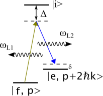
Figure 1: Representation of stimulated Raman transitions induced by two laser beams of frequencies $\omega_{\rm L1}$ and $\omega_{\rm L2}$. The Raman detuning is given by $\delta.$

Let us consider a particular realization of the process sketched in Fig. 1. Suppose that the atom is initially prepared in an internal state of energy $|f\rangle$ and momentum ${\bf p}$. After the absorption of a photon at frequency $\omega_{\rm L1}$ and the subsequent stimulated emission of a photon at $\omega_{\rm L2}$, the internal state of the atom is $|e\rangle$ and its momentum ${\bf p}+\hbar({\bf k}_{\rm L1}-{\bf k}_{\rm L2})$. Because the laser beams propagate in opposite directions, the atom changes its initial momentum by $2\hbar k$, where $2k=2|{\bf k}|=|{\bf k}_{\rm L1}-{\bf k}_{\rm L2}|$. To estimate the order of magnitude of the corresponding change in velocity, we consider a transition on the $D_{2}$ line of ⁸⁷Rb atoms. Along the axis of the Raman beams, the change in velocity is $2\times 5.9$ mm/s, which is twice the recoil velocity. This implies that, if the atom’s state changes from $|f,{\bf p}\rangle$ to $|e,{\bf p}+2\hbar{\bf k}\rangle$, then after one second its initial trajectory will be deflected by 1.2 cm.

By using light pulses (i.e., by changing the duration of the interaction between the atoms and the laser beams), any superposition state may be prepared between $|f,{\bf p}\rangle$ and $|e,{\bf p}+2\hbar{\bf k}\rangle$. In particular, the pulse duration that prepares a superposition of the states with the same weight for both states is called a “$\pi/2$” pulse and is used to implement a matter-wave beam splitter. If the light pulse exchanges the two states, then it is a “$\pi$” pulse and it implements a matter-wave mirror. Typically, these pulses have a duration of a few tens of microseconds for Raman beams with an optical power of about 400 mW and a 1/$e^{2}$ radius of 2 cm. The standard geometry of an atom interferometer is of Mach–Zehnder type with three light pulses, as shown in Fig. 2.

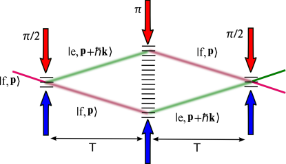
Figure 2: Mach–Zehnder atom interferometer configuration. The short, black, horizontal lines represent the equiphase planes of the laser beams in the laboratory frame, and $T$ is the free propagation time.

To determine the atomic phase $\Phi$ at the output of the AI, we measure the probability of detecting the atoms in states $|f,{\bf p}\rangle$ and $|e,{\bf p}+2\hbar{\bf k}\rangle$, which can be written as $P=A+B\cos(\Phi)$. For an apparatus subjected to an acceleration a, the phase $\Phi$ can be shown to be given by borde

$$\Phi_{\rm a}={\bf k}\cdot{\bf a}\ T^{2},$$ (1)

where $T$ is free propagation time between the laser pulses. If the device is subjected to a rotation at an angular rate ${\bf\Omega}$, then the atomic phase is

$$\Phi_{\Omega}=2{\bf k}\cdot({\bf\Omega}\times{\bf v})\ T^{2},$$ (2)

where ${\bf v}$ is the initial velocity of the atoms in the state $|f,{\bf p}\rangle$ at the AI input. The global inertial phase measured by an AI is therefore $\Phi=\Phi_{\rm a}+\Phi_{\Omega}$, which thus contains information about both the rotations and accelerations to which the device is subjected. This phase is imprinted by the laser beams onto the atomic wave function during the light-atom interactions that occur in the AI. Several techniques are available to isolate accelerations from rotations, the most common being to use a dual atom cloud source or a pulse configuration that renders the interferometer sensitive to rotations but not to DC accelerations. For instance, if a dual cloud source is used, then the two clouds are launched following reciprocal paths at exactly the same absolute velocity. In this situation, at the end of the interferometer sequence, the global inertial phase measured on one cloud carries a rotation contribution with velocity ${\bf v}$, whereas the measurement of the global phase on the other cloud gives a rotation contribution with velocity $-{\bf v}$. By adding and subtracting these two global phases, one may distinguish accelerations from rotations. How the global phase $\Phi$ is related to inertial forces is presented below.

II.2 Free-falling atom compact rotation sensors

Compact atom interferometer inertial sensors can be divided into three large classes: free-falling, confined, and guided atom interferometers. Out of these three classes, free-falling atoms define the state of the art, so we consider here a few representative implementations of this class. Almost all realizations of inertial sensing with AIs use free-falling cold atoms. The atoms are either dropped, launched vertically in a fountain configuration, or follow parabolic trajectories. In this way, the atoms provide an inertial frame with respect to which the forces exerted on the instrument can be measured. For example, in Fig. 2 the AI is sensitive to an acceleration in the direction of the Raman beams. On the one hand, accelerations translate into a displacement of the lasers’ equiphase planes (short black lines) with respect to the free-fall atomic trajectories. On the other hand, rotations of the equiphase planes with respect to the atomic trajectory and about an axis perpendicular to the AI’s oriented area are mapped to different light-atom interaction strengths in the phase of the atomic wave function at every light pulse.

One representative realization of a compact, free-falling AI was the first cold atom gyrometer realized by Canuel et al. at SYRTE. canuel This atom interferometer used a dual cloud source and measured the six inertial axes following the working principle presented in Fig. 3. It offered projection-noise-limited performance, with a sensitivity to rotations and accelerations of 2.4$\times$10^-7 rad s^-1 Hz^-1/2 and 5.5$\times$10^-7 m s^-2 Hz^-1/2, respectively. Despite this remarkable result, the performance of this device was limited by the initial temperature of the atoms (2 $\mu$K), the relatively short interrogation time ($2T=60$ ms), the small area ($\approx$4 mm²) of the interferometer, and the superposition of the atomic trajectories (Fig. 4).

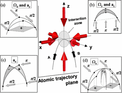
Figure 3: Principle of a six-axis inertial sensor. The atomic clouds are launched on a parabolic trajectory and interact with the Raman lasers at the top. The four configurations (a)–(d) give access to the three rotations and the three accelerations. In the three-pulse configuration, the Raman beam can be horizontal or vertical. Therefore, the atom cloud can be split or deflected in (a) the horizontal $x\text{-}y$ plane or (b), (c) in the vertical $x\text{-}z$ plane. (d) With a butterfly four-pulse sequence of horizontal beams, the rotation $\Omega_{x}$ can be measured. Adapted from Canuel et al., canuel © 2006 by the American Physical Society.

Figure 4: Picture of the SYRTE six-axis inertial sensor. The instrument is 50 cm tall. Courtesy of A. Landragin (Paris).

At NIST, Donley’s team recently demonstrated a multiaxis cold-atom gyrometer by using a single source in a centimeter-scale cell. chen Their device simultaneously measures accelerations and rotations by using a point source atom interferometer (PSI), as sketched in Fig. 5. After averaging for 1 s, the measured sensitivities for the magnitude of the rotation rate and the direction were $0.033^{\circ}$ s^-1 and $0.27^{\circ}$, respectively. Concerning acceleration measurements, the authors demonstrated a relative precision in the gravity measurement of $\delta g/g=1.6\times 10^{-6}$ Hz^-1/2. The PSI technique consists of an ensemble of single-atom independent interferometers.

Figure 5: Schematic of the PSI science package. The inner dimension of the glass cell is 1 cm². The instrument measures accelerations in the $z$ direction and the projection of the rotation vector onto the $x\text{-}y$ plane. “PBS” is a polarizing beam splitter. Adapted from Chen et al., chen © 2019 by the American Physical Society.

Because of the initial thermal velocity distribution of the cold atom cloud, a strong correlation exists between position and velocity after a ballistic expansion during the free-fall time of the cloud. This correlation means that two different atoms with exactly opposite velocities will interact with the Raman beams in the same way as the two clouds in the SYRTE gyrometer. It is this correlation that is exploited to measure distinguishably accelerations and rotations. Consequently, the PSI can be seen as a collection of dual-source atom interferometers, but at the single-atom level. The strength of the PSI is that it can measure rotation and acceleration in a single measurement shot and using a single atom cloud.

Typically, the measurement rate of an atom interferometer is on the order of a Hz. However, applications such as inertial navigation and guidance require a high measurement bandwidth for the proper real-time integration of the vehicle equations of motion. At Sandia National Laboratories, Rakholia et al. rakholia tackled this critical question and realized a dual-axis device with a 60 Hz bandwidth. The core idea of their technique is based on combining a dual atomic source with the recapture of a fraction of the atoms after the interferometer sequence. By simultaneously measuring accelerations and rotations, this work presents a building block of a six-axis inertial sensor. Although the interferometer duration is relatively short (4 ms), the loss in sensitivity is compensated by using large atom numbers, large launching velocities, and reducing the dead time. The measured sensitivities, which are typical of laboratory experiments, are in the range of $\mu g$ Hz^-1/2 and $\mu$rad s^-1 Hz^-1/2 for acceleration and rotation, respectively. Such performance is the result of a carefully developed device, analyzed following a model developed by the authors. The identification and characterization of the various noise sources also contributed to achieving the high sensitivities shown in this work.

Another example of free-falling compact atom gyrometers was developed at Hannover in Rasel’s group. tackmann Their gyrometer had a Sagnac area of 19 mm² and was 13.7 cm long. The rotation measurement was performed by using a cold atom beam at 2.79 m s^-1 and achieved a sensitivity of 6.1$\times$10^-7 rad s^-1 Hz^-1/2.

At Bordeaux, Barrett et al. developed a dual-species ⁸⁷Rb-³⁹K compact inertial sensor for the study of the equivalence principle in microgravity. barret One of the important achievements of this experiment, from the inertial-sensing perspective, is the operation of an atom interferometer in the strongly vibrating environment of an aircraft. The sensor, subjected not only to vibration levels of 10^-2 $g$ Hz^-1/2 but also to rotation rates as large as $5^{\circ}$ s^-1, measured the Eötvös ratio in microgravity with a systematic uncertainty of 3$\times$10^-4.

III Guided atom interferometry with atom chips

III.1 Main requirements for navigation

For an inertial navigation application, the main constraints for an atom interferometer are small volume, low power consumption, high bandwidth, high dynamic range, low cost, robustness, and device survivability when exposed to or operated in a severe environment. barbour The sensor is then suitable for a specific inertial navigation task depending on its performance. For instance, the angular random walk of a navigation-grade gyrometer has to be less than $10^{-3}{}^{\circ}\,\text{h}^{-1/2}$.

To use an atom chip as a sensor platform, several technological obstacles have to be addressed. Whether trapped or guided, coherent splitting and recombination of a sub-Doppler–cooled thermal or degenerate atomic ensemble is required. If we use a trapped ensemble, then symmetric splitting at the level of 10^-3 is required to have coherence times greater than 40 ms, and acceleration must be sensed at the 10${}^{-6}~{}g$ level. In the case of a guided atom interferometer, we need to fabricate or somehow generate equivalent roughness-free matter-wave guides. For rotation sensing, the phase bias stability has to be at the 10${}^{-4}{}^{\circ}\,{\rm h}^{-1}$ level.

III.2 Enabling technologies

Atom chip technology has been extensively covered in several reviews. keil ; fortagh ; folman ; folman1 ; lev ; reichel Here, we address the atom chip enabling technologies relevant to key functional building blocks necessary for implementing compact inertial sensors with cold guided atoms. These functions concern

• the precise and accurate positioning of the atoms to start the interferometer sequence;

• the coherent momentum transfer and splitting of the atom clouds;

• the attenuation or suppression of propagation-induced decoherence;

• the on-chip detection;

• the vacuum dynamics because of its non-negligible contribution to the Dick effect dick via sensor dead time.

Addressing these points is important in order to exploit the full potential for compactness offered by an atom chips.

Atom chips are a promising technology for manipulating cold atoms using complicated confining geometries, which is important for developing compact matter-wave interferometers. keil In fact, it is possible to microfabricate on an atom chip a complex wire pattern to create sub-micron magnetic potentials with the shape required by the targeted application. We can, for example, design arrays of potential wells for quantum information processing, sinuco traps for measuring accelerations, ammar and toroidal waveguides for detecting rotations. clga ; lesanovsky ; fernholz ; seungjin

The coherent beam splitting of a cold thermal cloud has already been demonstrated for propagating atoms. cassetari On atom chips, the coherent manipulation of Bose–Einstein-condensed trapped and propagating atoms has been observed in atom interferometers schumm ; maussang ; shin ; wang and atomic clocks. treutlin ; deutsch

Although cold atom propagation in circular macroscopic guides has already been observed, gupta ; gildemeister the demonstrated sensitivity to rotations was insufficient for high-precision measurements or inertial sensing applications. Using a linear waveguide, Wu et al. estimated the expected rotation sensitivity of their enclosed-area interferometer. wu Although the estimated short-term sensitivity was 1$\times$10^-9 rad s^-1 Hz^-1/2, the expected stability was insufficient for measurements at a metrologically relevant level. In other work, Qi et al. qi built a magnetically guided atom interferometer that uses Cs atoms and for which they used a compact architecture to measure accelerations. The guide was generated by race-track coils carrying a current of about 30 A. The resulting magnetic guide had a radial frequency of 98 Hz and was loaded with 5$\times 10^{7}$ Cs atoms. The resulting measurement uncertainty was 7$\times 10^{-5}$ m s^-2 with an interrogation time of $2T$ = 18 ms. The guide had an enclosed area of 1.8$\times 10^{-2}$ mm² and can potentially be used to sense rotations.

Atom chips offer a convenient and flexible way for precise spatial positioning of the atom clouds at the input port of the interferometer. Long et al. used a magnetic conveyor to transport atoms over a total distance of 24 cm. long Figure 6 shows the operation of this conveyor, which rotates the atom cloud position by 90^∘.

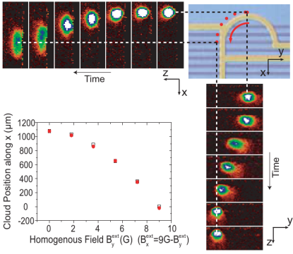
Figure 6: Illustration of positional precision that can be realized by using an atom chip. The figure shows the rotation of a cloud of trapped ⁸⁷Rb atoms. The absorption images were acquired along two perpendicular axes parallel to the substrate. The pictures are scaled so that the wire dimensions may serve as a length scale for determining the cloud size. Reprinted with permission from Long et al., long © 2005 by Springer Eur. Phys. J. D.

Another relevant development for guided atom interferometry is their demonstration of a magnetic guide that does not require an external bias field. The guide is loaded by the rotating-trap device shown in Fig. 6. In other work, Günther et al. demonstrated sub-micron accuracy in detecting the position of a Bose–Einstein condensate, gunther which enabled a demonstration of magnetic-field microscope sensing at the mG level.

Different atom interferometer techniques are available to launch atoms into the guide by subjecting them to a momentum kick. For magnetically guided atoms, the standard solution is to use double Bragg diffraction. swu ; giese In particular, Wu et al. developed a theory to describe a pulse sequence of two square-shaped standing-wave light pulses. swu By properly choosing the strengths, durations, and separation between pulses, a Bose–Einstein condensate at rest may be almost perfectly (99%) split into the $\pm 2\hbar k$ diffraction orders. wang ; swu Figure 7 shows the designed pulse sequence.

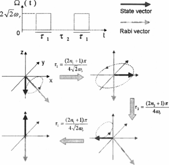
Figure 7: (top) Illustration of the two square-shaped pulse sequence. (bottom) Representation of the momentum-state vector in the Bloch sphere. Adapted from Wu et al., swu © 2005 by the American Physical Society.

On atom chips, coherent momentum splitting can be produced by using a Stern–Gerlach beam splitter, as demonstrated by Machluf et al. in Ref. machluf, . The beam splitter results from a combination of magnetic-field gradient pulses and RF transitions between Zeeman states. Both the gradient and the RF field are generated by feeding current to on-chip wires. Figure 8 shows absorption images of the splitting process.

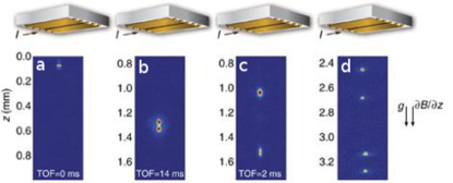
Figure 8: Time-of-flight absorption images (a) of the trapped cloud. In panel (b), the momentum splitting is weak (less than $\hbar k$) when using 5 $\mu$s of interaction time with the magnetic-field gradient ($\text{TOF}=14$ ms). The splitting realized in panel (c) corresponds to $40\hbar k$ of momentum transfer using 1 ms interaction time and 2 ms TOF. In panel (d), the absorption images show when the internal states are separated by an additional strong gradient pulse. Adapted from Machluf et al., machluf © 2013 by Springer Nature Communications.

In this work the authors demonstrate interference fringes characterized by short-term phase fluctuations of about 1 radian and long-term drifts on the time scale of an hour. State-dependent microwave potentials can also be used to induce momentum transfer with on-chip microfabricated wires. bohi

Usually, the number of atoms after application of the final beam-splitter pulse is used to determine the inertial phase at the end of a single AI cycle. This is done for all the propagation modes in order to compute the associated probabilities, as discussed in Sec. IV. The standard technique is based on absorption imaging, as already presented, for instance, in Fig. 6. However, locally detecting atoms at well-defined positions on the chip is advantageous for three main reasons: The first reason is that individual manipulation of the atom clouds (or single atoms) becomes possible, which can be useful for preparing one atom cloud and, at the same time, measure the AI output on the previously prepared cloud. This would allow, for example, an interleaved operation configuration. savoie The second reason is the possibility to implement local quantum non-demolition measurements of atom number at the AI output. Such a strategy would allow recycling of atoms in the interferometer to increase its measurement bandwidth. Finally, the third reason is that integrated atom detection can be implemented (for instance, in situ collection of fluorescence by using an on-chip fiber), which is important for making compact sensors and avoiding the use of CCD cameras.

The enabling technology in this case has already been demonstrated by using integrated optical elements on an atom chip. wilzbach Another solution is to combine an atom chip with integrated photonic optical chips. In both situations, atoms may be locally excited for position-resolved detection. ritter ; mehta ; mehta1 ; kohnen Figure 9 shows a schematic representation of an optical chip used to acquire the spectrum of a hot vapor of rubidium atoms. It is based on a Mach–Zehnder light interferometer with one arm exposed to the atomic vapor. The evanescent field of the optical waveguide mode interacts with the atoms, and the interaction strength is read out as a modification of the interferometer transmission. In other words, the presence of the atoms produces a phase shift that carries information on their number and internal state.

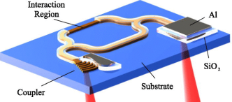
Figure 9: Schematic drawing of an integrated Mach–Zehnder optical interferometer containing an interaction or detection region for the atoms in one of its arms. Light is coupled in by focusing a laser beam onto a grating coupler. Another grating coupler is used to extract the light from the device. Reprinted with permission from Ritter et al., ritter © 2015 AIP Publishing LLC.

In another experiment, Mehta et al. used a grating coupler to implement position-resolved excitation of ions mehta1 and addressed a single ⁸⁸Sr⁺ qubit, as shown in Fig. 10.

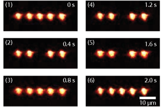
Figure 10: Fluorescence images showing single-ion addressing. The grating coupler is aligned with the central ion, which is prepared in a dark state by focusing a 674 nm laser onto the grating. The fluorescence is at 422 nm, and the signal is collected for 2 s. Adapted from Mehta et al., mehta1 © 2016 by Springer Nature Publishing AG.

To guarantee monomode propagation of guided atoms golding ; andersson ; burke1 ; das ; wu1 when realizing magnetic waveguides with relatively low currents (below hundreds of mA), the atoms must be confined close to the chip surface. However, in this situation, the coherent properties of the atomic states can be dramatically affected by the corrugation of the microwires. These fabrication defects produce a magnetically rough potential that can destroy the system coherence or, even worse, blockade the propagation of the atoms. kruger ; Whitlock ; sinclair:031603 Fabrication defects have been a fundamental limitation for atom chips. kraft ; Hinds ; leanhardt:100404 ; EstevePRArug ; lukin ; sculturing ; EsteveDWell The physical origins of this roughness can be understood as follows: Consider a wire with a current flowing left to right as shown by the dark blue arrow in Fig. 11.

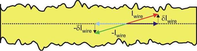
Figure 11: Top view of current $I_{\rm wire}$ flowing in a wire with corrugated walls.

Because of meanders in the wire’s wall, an electron flux exists in the direction perpendicular to the wire. These electrons generate a current $\delta I_{\rm wire}$ that in turn produces a magnetic trapping potential in the direction parallel to the wire.

Figure 12(a) shows an in-trap absorption image of a cold thermal ⁸⁷Rb cloud that exhibits fragmentation. This image corresponds to atoms loaded in a linear magnetic guide created with three microfabricated wires, trebbia each of which carried a DC current in a configuration that creates a quadrupole trap close to the minimum of the guiding potential. When the current directions are reversed, the extrema of the rough magnetic potential are also reversed, as can be seen in Fig. 12(b). However, the atoms are now confined in complementary positions with respect to Fig. 12(a), and

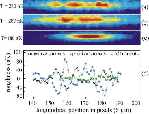
Figure 12: (a) Absorption images of a thermal cloud for negative DC, (b) positive DC, and (c) AC currents. Plotted is the number of atoms per pixel (pixel size is $6\times 6~{}\mu$m²). Panel (d) shows the potential roughness extracted from longitudinal profiles by using the Maxwell–Boltzmann distribution. Adapted from Trebbia et al., trebbia © 2007 by the American Physical Society.

it is this complementarity that inspired the modulation technique that suppresses the roughness of the magnetic guide. trebbia In fact, by temporally modulating the current in the wires, Trebbia et al. demonstrated a roughness-free guide, as can be seen in the absorption image shown in Fig. 12(c). The rough potential was extracted by fitting the linear density with a Maxwell–Boltzmann distribution along the axis of the cloud in Figs. 12(a)–12(c). bouch This result is presented in Fig. 12(d), which quantifies the fragmentation complementarity observed in the previous figures and the degree of suppression of the roughness. For this technique to work, two criteria must be satisfied: (a) the modulation frequency must exceed the radial guide frequency but not the Zeeman frequency; (b) the phase difference between the currents must be constant.

One of the key components of any cold atom sensor is the vacuum system. The simplest vacuum setup would use a single chamber incorporating the atom source (i.e., an alkali-metal dispenser). However, this solution requires a highly dynamic vacuum system capable of switching from high (${\approx}10^{-8}$ mbar) to low pressure (${\approx}10^{-11}$ mbar) in a few tenths of milliseconds. Dugrain Such a response is needed to reduce the deleterious effect of the dead time between measurements. Recently, a promising technique was demonstrated kitching that allows one to quickly and reversibly control the Rb background pressure in a cell, with switching times close to 1 s. This reversible operation is illustrated in Fig. 13, where the magneto-optical-trap (MOT) loading and depletion are controlled by a voltage applied across the electrodes.

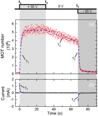
Figure 13: (a) MOT time response is represented by experimental points (red dots), which correspond to the measured atom number. (b) The current flowing in this reversible source is given by the black points. Adapted from Kang et al., kitching © 2019 by the Optical Society of America.

Other relevant investigations on the optimized operation of compact ultrahigh vacuum (UHV) systems have been reported in Ref. campo, . In this work, light-induced atomic desorption is used to modulate the background pressure of ⁸⁷Rb atoms in a glass cell. For atom interferometry and atom sensors, a UHV system was designed and tested for operation in the highly vibrating environment of a rocket. grosse In Ref. scherer the authors investigated the use of passive vacuum pumps (non-evaporable getter pumps) for the development of compact cold atom sensors. Basu and Velásquez-Garcia basu demonstrated microfabricated non-magnetic ion pumps to maintain UHV conditions in miniature vacuum chambers for atom interferometry. Finally, Martin et al. jmm investigated the pumping dynamics of sputtered ion pumps. This study describes the main physical pumping mechanisms based on a nonlinear model for the ion-current pump-down dynamics in the low-pressure regime. The results suggest that a three-dimensional (3D) structured cathode might allow for a smaller pump, increasing or at least holding constant the trapping cross section of this electrode, which may have significant consequences on the design and development of miniature ion pumps.

IV Case study of a sensor design

This section presents a case study of a rotation sensor design that uses an atom chip. The working principle is based on the Sagnac effect, which naturally suggests a circular guiding geometry for the AI.

IV.1 Measuring rotation with a waveguide

To establish the physics that will drive the gyrometer design, consider the Sagnac effect as sketched in Fig. 14. Starting with the illustration on the left side of the figure, assume that, at $t=t_{0}$, two particles $A$ and $B$ leave the AI entry port $E$ and propagate freely in the azimuthal direction of this circular guide of radius $r$. If the guide is rotated about an axis ${\bf\Omega}$ perpendicular to the guide’s oriented area, then after a time interval $\delta t$ particles $A$ and $B$ would travel a geometrical path length $\delta_{A}=r(\pi-\Omega\delta t)$ and $\delta_{B}=r(\pi+\Omega\delta t)$, respectively. Therefore, there exists a path-length difference $\delta_{AB}=\delta_{B}-\delta_{A}$ determined by the different arrival times of the particles at the exit port $S$. By measuring this quantity, we can determine the magnitude and direction of the rotation of the apparatus.

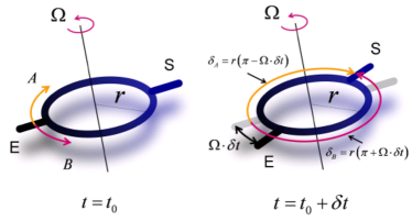
Figure 14: Illustration of the Sagnac effect in a circular guide.

In the following, we discuss the key elements of the design of an atom-chip-based cold atom gyrometer. To be quantitative, we consider magnetic guiding of ultracold thermal ⁸⁷Rb atoms.

IV.2 Sensor design

Guiding

As we have seen, several solutions exist for realizing a matter-wave guide. To implement an inertial sensor and exploit the potential for compactness offered by an atom chip, we consider a circular magnetic guide produced by three on-chip microfabricated concentric wires. Figure 15 shows the wire pattern, which does not require an external bias field produced with coils. This is a well-known configuration in which the external wires generate the bias magnetic field needed to cancel the magnetic field of the central wire.

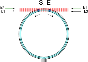
Figure 15: Microfabricated-wire configuration used to generate the circular magnetic guide shown in Fig. 16. Here, the entry $E$ and output $S$ ports are located at the same point in space. The laser beams implementing the matter-wave optics are represented by the wave vectors ${{\bf k}_{1}}$ and ${{\bf k}_{2}}$.

The resulting field is a quadrupole field and, by modulating the current fed to the wires, the atoms can be guided at the minimum of this field in an equivalent roughness-free stable magnetic guide. trebbia ; clgapra Note that the entry $E$ and output $S$ ports are located at the same point in space. Such a geometry allows rejection of common-mode noise. Figure 16 shows the magnetic potential generated by this configuration of microfabricated wires. This magnetic potential is obtained when the wires are separated by 13 $\mu$m and carry modulated currents of $-123$ mA and 121 mA in the external and central wires, respectively. The radius of the central wire is $R=500~{}\mu$m. The magnetic guide obtained in this way is around 13 $\mu$m from the chip surface.

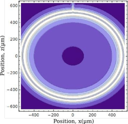
Figure 16: Magnetic guiding potential for on-chip cold atom gyrometer. It is produced by a three-wire configuration in which the distance between the wires is 13 $\mu$m and the central circular wire has a radius of 500 $\mu$m.

Given these parameter values, the radial guiding frequency is about 1.5 kHz, and the potential depth is roughly 300 $\mu$K. These guide design parameters allow the propagation of cold thermal atoms. By using this type of source we can avoid the important contribution of atom-atom interactions to the systematic noise and drift in the inertial phase of interest, wang ; horikoshi ; jo ; li ; stickney and less preparation time is required than with Bose–Einstein-condensed samples. In fact, concerning just the cooling process, cold thermal atoms used in atom interferometry are obtained after molasses cooling whereas degenerate samples require an additional evaporative-cooling step. However, quantum degenerate atom sources might be relevant when realizing, for instance, large-momentum-transfer beam splitters. mcdonald ; debs Actually, as discussed later, the sensitivity of the interferometer can be enhanced by increasing the launch velocity and by letting the atoms undertake several trips around the guide at a fixed single-loop interrogation time $2T$.

Guide fabrication

The realization of the proposed configuration, shown in Fig. 15, raises several fabrication challenges. For instance, the fabrication of the microwires must account for the relevant practical and physics constraints of a compact sensor for inertial navigation. From the practical point of view, power consumption is another relevant constraint (for instance, to operate the sensor on batteries). As already discussed, this problem can be mitigated by guiding the atoms close to the chip surface, at a few tens of microns. In this case, the proximity to the chip allows the production of strong magnetic-field gradients to confine the atoms by using currents well below 1 A. note2 This point is important for two main reasons: First, reducing the current intensity reduces the heat dissipated by the wires. Second, developing or adding a heat-management solution to the sensor, which can be detrimental to its performance, is not necessary (e.g., a cooling system that introduces parasitic vibrations). However, from the physics point of view, as already mentioned, the proximity to the wires renders the guided atoms sensitive to the roughness of the magnetic potential. This problem suggests a microfabrication process based on metal evaporation, but this is a costly solution when considering mass production of these sensors. The combined challenge of low roughness and low cost can be addressed by using a metallization process based on electroplating. The only requirement that remains in this case is the realization of relatively small metal grains. lev In addition, using an electroplating process allows the fabrication of microwires with cross sections with large aspect ratios. In this way, their electrical resistance and, consequently, heat dissipation can be reduced.

Figure 17 shows an example of a circular magnetic guide used to transport atoms from the laser-cooling region to the science region of an atom chip. huang The picture illustrates a three-wire circular geometry of 1 cm diameter in which the atoms are transported at 240 $\mu$m from the atom chip surface, which demonstrates the feasibility of fabricating the wire pattern needed to produce circular magnetic guiding potentials on an atom chip. The bottom chip is used to realize an evaporative cooling trap and also serves as an electrical feedthrough for the in-vacuum wires of the top chip in which the circular trap is implemented. Both atom chips were fabricated by using electroplating, which is a well-established technology in the microelectronics industry.

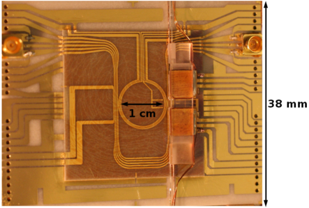
Figure 17: Photograph of the atom chip of the LKB-SYRTE experiment Trapped Atom Clock on a Chip. The experiment is developing an entanglement-enhanced atomic clock with trapped atoms on a chip. More details are available in Ref. huang, . Courtesy of J. Reichel (Paris).

Scale factor

When using magnetically guided atoms, it is preferable to use Bragg transitions giltner ; ahlers to realize the beam-splitter and mirror light pulses. moler In fact, in a Bragg transition, only the atomic momentum is modified and the atoms remain in the same magnetic-trappable internal state. In a circular waveguide, only beam-splitter pulses need be implemented because the atomic trajectories are, by construction, deflected by the guide. For the geometry shown in Fig. 15, we require only two Bragg transitions, as indicated in Fig. 18. If we do not use a composite pulse sequence, swu the initial state $|\Psi\rangle=|{\bf p}=0\rangle$ is transformed into a three-component superposition state $|\Psi\rangle=\alpha|{\bf p}=-2\hbar{\bf k}\rangle+\beta|{\bf p}=+2\hbar{\bf k}\rangle+\gamma|{\bf p}=0\rangle$.

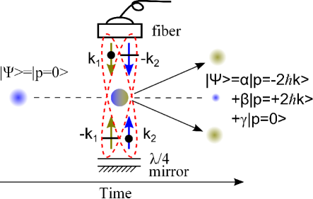
Figure 18: Beam-splitting process for the circular guiding potential considered in Fig. 15. It represents a double Bragg diffraction, ahlers each realized by the pair of beams enclosed by a given red dashed ellipse.

By using the path-integral approach, pippa one can show that the relevant inertial (rotation) phase defining the scale factor is given by the expression

$$\Phi=4kR\Omega(2T)=2\times 2\frac{M}{\hbar}A\Omega,$$ (3)

where $2T=\pi R/v_{\rm r}=M\pi R/(\hbar k)$ is the interferometer interrogation time for a round trip in a guide of area $A=\pi R^{2}$ and $v_{\rm r}$ is the recoil velocity. In Eq. (3), we have considered an ideal beam-splitting process to compute the probability of finding the atoms at the output port $|{\bf p}=0\rangle$ of the AI.

Rotation-rate sensitivity

When the AI is operated at mid-fringe (maximum phase sensitivity), the probability $P(\Omega)$ of finding the atoms at the output port $|{\bf p}=0\rangle$ is

$$P(\Omega)=\frac{N}{2}\big{[}1-\eta\cos\big{(}\Phi+\pi/2\big{)}\big{]},$$ (4)

where $N$ and $\eta$ are the number of atoms and the contrast of the AI, respectively. Equation (4) states that an infinitesimal variation of $P(\Omega)$ translates into an infinitesimal variation of the rotation rate such that

$$\delta\Omega=\frac{1}{\Big{|}\frac{dP(\Omega)}{d\Omega}\big{|}_{\Omega=0}\Big{|}}\delta P(\Omega=0).$$ (5)

In Eq. (5), $\delta P(\Omega=0)$ gives the probability noise around the working point of the AI, which can be chosen, for example, by setting a fixed phase difference between the Bragg beams. For instance, in Eq. (4) the phase difference is $\pi/2$, such that $P(\Omega)$ is the half-fringe value of the interference signal in the absence of rotations. If we represent by $\vartheta$ the latitude on Earth where the instrument is located, then Eq. (3) becomes

$$\Phi=\frac{4}{\pi}\frac{M}{\hbar}v_{\rm r}^{2}(2T)^{2}\Omega\sin(\vartheta),$$ (6)

and consequently we have

$$\frac{dP(\Omega)}{d\Omega}\Big{|}_{\Omega=0}=\frac{2}{\pi}N\eta\frac{M}{\hbar}v_{\rm r}^{2}(2T)^{2}\sin(\vartheta).$$ (7)

If the probability noise is defined solely by the quantum projection noise, then

$$\delta P(\Omega=0)=\sqrt{P(\Omega=0)}=\sqrt{\frac{N}{2}},$$ (8)

so we finally find the following expression for the rotation-rate sensitivity:

$$\delta\Omega=\frac{\pi}{2\eta\sqrt{2N}(M/\hbar)v_{\rm r}^{2}(2T)^{2}\sin(\vartheta)}.$$ (9)

Physically, Eq. (9) gives us the minimal rotation rate that can be detected if the AI is projection-noise limited. To reach the projection-noise-limited sensitivity, several technical problems must be overcome. In particular, for a magnetic guide produced with modulated currents, the relative stability of the currents supplied to the microwires and the noise level of the phase difference between them must be considered. Both noise sources induce a fluctuation in the separation between the guide and the chip surface. reichel Consequently, the radial frequency of the guide (i.e., the radial confinement energy of the guide) also fluctuates, generating a phase noise that is mapped to the phase of the atomic wave function. As a result, the measured inertial phase will acquire a parasitic contribution due to these physical effects. In addition, if the guide uses a self-generated offset field, clgapra then the phase fluctuations will also compromise the stability of the magnetic guide. Other relevant problems limiting the sensitivity and accuracy of this device, and that are common to cold atom sensors, are detection noise, magnetic-field noise, cloud temperature, and shot-to-shot atom number fluctuations (see, for instance, Ref. szmuk, ).

As an example, Fig. 19 plots the rotation sensitivity given by Eq. (9) versus the interferometer interrogation time and for a fixed launching velocity 2$v_{\rm r}$, which means that the guide radius depends on the interferometer duration under consideration.

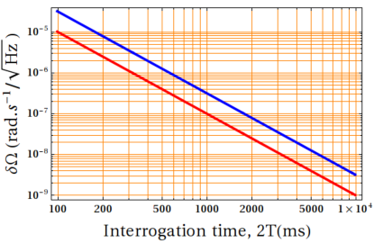
Figure 19: Calculated interferometer rotation-rate sensitivity vs interrogation time. The red (blue) line is for $N=10^{5}\ (10^{4})$ atoms and perfect visibility ($\eta=100\%$).

The result presented in Fig. 19 indicates that, for instance, using $10^{4}$ atoms and an interferometer duration $2T=3$ s gives a short-term rotation sensitivity of $3.4\times 10^{-8}$ rad s ${}^{-1}{\rm Hz}^{-1/2}$ or an angular random walk, $ARW\approx 1.1\times 10^{-4}{}^{\circ}\,{{\rm h}}^{-1/2}$. In other words, after 1 h of integration the angular standard deviation will be $1.1\times 10^{-4}{}^{\circ}$. Such a rotation-rate sensitivity can be realized by using a 6-mm-radius guide or after 10 round trips in a 600-$\mu$m-radius guide. For defense applications, this ARW is already compatible with strategic-grade inertial navigators.

Sensitivity function

This function is defined as

$$g(t)\equiv 2\lim_{\delta\phi\to 0}\frac{\delta P}{\delta\phi},$$ (10)

where $\delta P$ is the infinitesimal variation of the probability $P$ of finding the atoms at the AI output port. This variation results from an infinitesimal jump of the global phase $\delta\phi$ due to a perturbation during the measurement process.

The function $g(t)$ is a measure of the impact of a given perturbation, which happens during the interrogation time $2T$, on the determination of the atomic phase. cheinet In fact, inside the time window defined by $2T$, the global phase is sensed only during the time interval defined by the beam-splitter and mirror light pulses. Therefore, we expect the sensitivity function to vary during the pulses and to be extremal between them. The simplest gyrometer configuration realized with a circular magnetic guide uses two $\pi/2$ pulses of duration $\tau$, applied at the beginning and at the end of the AI. Therefore, the sensitivity function of this device has the form presented in Fig 20.

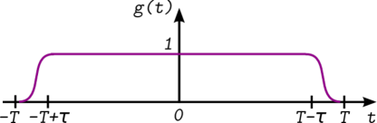
Figure 20: Sensitivity function for the circular guide shown in Fig. 15.

Transfer function

To determine the transfer function we compute the interferometer phase noise $\sigma_{\phi}^{2}$. We denote by $\overline{\Delta\phi}$ the difference of the mean phases during the pulses:

$$\overline{\Delta\phi}(\tau)\equiv\overline{\phi}_{2}(\tau)-\bar{\phi}_{1}(\tau),$$ (11)

where

$$\overline{\phi}_{1}(\tau)=\frac{1}{\tau}\int_{-T}^{-T+\tau}dt\phi(t),\quad\overline{\phi}_{2}(\tau)=\frac{1}{\tau}\int_{T-\tau}^{T}dt\phi(t).$$ (12)

In this case, the phase noise measured during the pulses is

$$\sigma_{\phi}^{2}=\Big{\langle}\Big{|}\frac{1}{\tau}\int_{T-\tau}^{T}dt\phi(t)-\frac{1}{\tau}\int_{-T}^{-T+\tau}dt\phi(t)\Big{|}^{2}\Big{\rangle}_{T},$$ (13)

where $\sigma_{\phi}^{2}=\big{\langle}\big{|}\overline{\Delta\phi}(\tau)\big{|}^{2}\big{\rangle}_{T}$ and $\langle\dots\rangle_{T}$ is the temporal mean evaluated over a time interval equal to the interrogation time $2T$. Here, $\phi(t)$ is the instantaneous phase “seen” by the interferometer (resulting from rotations, vibrations, laser phase noise, etc.).

From Eq. (13), the transfer function of this AI in the time domain is $h(t)$, which is shown in Fig. 21 and defined as follows:

$$h(\tau-t)\equiv\left\{\begin{array}[]{rl}0,&|t|<-T\\ 1/\tau,&-T\leq t\leq-T+\tau\\ 0,&-T+\tau<t<T-\tau\\ -1/\tau,&T-\tau\leq t\leq T.\end{array}\right.$$

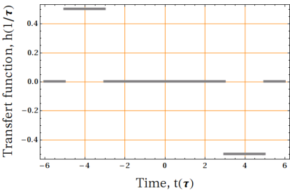
Figure 21: Time-domain transfer function of a two-pulse AI rotation sensor.

The transfer function $h(t)$ expresses the fact that the AI behaves as a bandpass filter with characteristic frequencies defined by $\tau$ and $T$.

In the frequency domain, the transfer function $H(f)$ can be easily computed and is given by the expression

$$H(f)=-\frac{2\imath}{\pi f\tau}\sin(\pi f\tau)\sin\big{[}(\pi f(2T-\tau)\big{]}.$$ (14)

The transfer function is presented in Fig. 22 for experimentally accessible parameter values. The cutoff frequencies are given by $f_{HP}\equiv 1/(\pi\tau)$ and $f_{LP}\equiv 1/[\pi(2T-\tau)]$. As can be seen in Fig. 22, an ensemble of frequencies exists at which the interferometer is not sensitive to phase noise. These frequencies correspond to multiples of the inverse of the pulse duration and the interrogation time.

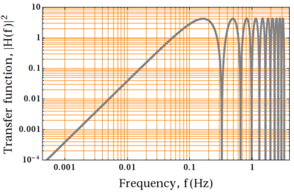
Figure 22: Frequency-domain transfer function of a two-pulse AI. To obtain this plot, we consider a pulse duration $\tau=20~{}\mu$s and an interrogation time $2T=4$ s. The cutoff frequencies are $f_{HP}=15.9$ kHz and $f_{LP}=0.1$ Hz.

IV.3 Main sources of noise and systematic effects

Phase noise expressed via the transfer function

By using the time-domain transfer function, Eq. (13) can be written as

$$\sigma_{\phi}^{2}=\Big{\langle}\Big{|}\int_{-\infty}^{+\infty}dt\phi(t)h(\tau-t)\Big{|}^{2}\Big{\rangle}_{T}=\big{\langle}\big{|}\phi(t)\otimes h(t)\big{|}^{2}\big{\rangle}_{T},$$ (15)

or, making explicit the temporal mean,

$$\sigma_{\phi}^{2}=\lim_{T\to\infty}\frac{1}{2T}\int_{-T}^{T}dt\big{|}\phi(t)\otimes h(t)\big{|}^{2}.$$ (16)

For practical purposes, we write the phase noise in terms of the interferometer spectral properties, its frequency domain transfer function $H(f)$, and the power spectral density (PSD) of the phase noise, $S_{\phi}(f)$. By using Parseval’s theorem and the definition of $h(t)$, Eq. (16) takes the form

$$\sigma_{\phi}^{2}=\lim_{T\to\infty}\frac{1}{2T}\int_{-\infty}^{+\infty}dt\big{|}\phi(t)\otimes h(t)\big{|}^{2}\operatorname*{\Longleftrightarrow}^{\rm Parseval}_{\rm theorem}\ \lim_{T\to\infty}\frac{1}{2T}\int_{-\infty}^{+\infty}df\big{|}\phi_{T}(f)\big{|}^{2}\big{|}H(f)\big{|}^{2},$$ (17)

where $\phi_{T}(f)$ denotes the Fourier transform of $\phi(t)$. Therefore, if $S_{\phi}(f)$ is the PSD of the phase noise, then we obtain

$$\sigma_{\phi}^{2}=\int_{0}^{+\infty}dfS_{\phi}(f)\big{|}H(f)\big{|}^{2}.$$ (18)

Sensitivity of AI phase to laser phase noise

To characterize the noise in the phase accumulated during the interferometer interrogation time $\Phi$, we use the sensitivity function. Recall that, for a 100% contrast interferometer operating at mid-fringe, the probability $P$ at the output port is

$$P=\frac{1}{2}\big{[}1-\cos(\Phi+\pi/2)\big{]}.$$ (19)

Consequently, the variation of $P$ due to an infinitesimal phase jump of the Bragg laser is

$$\frac{\delta P}{\delta\phi}=\frac{1}{2}\sin(\Phi+\pi/2)\Big{|}_{\Phi=0}\frac{\delta\Phi}{\delta\phi}=\frac{1}{2}\frac{\delta\Phi}{\delta\phi},$$ (20)

from which the sensitivity function associated with a phase jump becomes

$$g_{\phi}(t)=\lim_{\delta\phi\to 0}\frac{\delta\Phi}{\delta\phi}.$$ (21)

Thus, the measured accumulated AI phase during the interrogation time $2T$ is

$$\Phi=\int_{-T}^{T}dtg_{\phi}(t)\frac{d}{dt}(\delta\phi),$$ (22)

and consequently the phase noise after one interferometer cycle is

$$\sigma_{\Phi}^{2}=\Big{\langle}\Big{|}\int_{-T}^{T}dtg_{\phi}(t)\frac{d}{dt}(\delta\phi)\Big{|}^{2}\Big{\rangle}_{T}.$$ (23)

By using the definition of the sensitivity function (Fig. 20) and considering that this function vanishes outside the interval $[-T;T]$, we find

$$\sigma_{\Phi}^{2} = \lim_{T\to\infty}\frac{1}{2T}\int_{-\infty}^{+\infty}dt\big{|}g_{\phi}(t)\otimes\frac{d}{dt}(\delta\phi)\big{|}^{2}$$ (24)

$$= \lim_{T\to\infty}\frac{1}{2T}\int_{-\infty}^{+\infty}d\omega\big{|}G(\omega)\big{|}^{2}\big{|}\omega\ \delta\phi_{T}(\omega)\big{|}^{2},$$

and finally

$$\sigma_{\Phi}^{2}=\int_{0}^{+\infty}d\omega S_{\phi}(\omega)\omega^{2}\big{|}G(\omega)\big{|}^{2}.$$ (25)

Comparing Eq. (18) with Eq. (25) shows that the frequency-domain transfer function of the AI and the Fourier transform of the sensitivity function $G(\omega)$ are linked by

$$\big{|}H(\omega)\big{|}^{2}=\omega^{2}\big{|}G(\omega)\big{|}^{2}.$$ (26)

In addition, considering Eqs. (6) and (25), the rotation rate measured by the AI may be characterized by the standard deviation

$$\sigma_{\Omega}=\frac{\pi}{4}\frac{\hbar}{M}\frac{1}{v_{\rm r}^{2}(2T)^{2}\sin(\vartheta)}\sigma_{\Phi}.$$ (27)

Sensitivity to vibrations or acceleration noise

We have previously seen that the AI accumulated phase is [since $g_{\phi}(t)=0\ \forall\ t\notin[-T;T]$ ]

$$\Phi=\int_{-\infty}^{+\infty}dtg_{\phi}(t)\frac{d}{dt}(\delta\phi).$$ (28)

In the case of Bragg transitions with counterpropagating laser beams in the $z$ direction, the phase (wavefront or equiphase plane) at the location of the atoms and at time $t$ is $\phi(t)=2kz(t)$. Thus,

$$\Phi=2k\int_{-\infty}^{+\infty}dtg_{\phi}(t)\frac{d}{dt}(\delta z).$$ (29)

Computing the integral in Eq. (29) gives

$$\Phi=\int_{-\infty}^{+\infty}dt\Bigg{[}-2k\int_{-\infty}^{t}dt^{\prime}g_{\phi}(t^{\prime})\Bigg{]}\delta\Big{(}\frac{d^{2}z}{dt^{2}}\Big{)},$$ (30)

which leads to the following definition of the sensitivity function of the AI to accelerations:

$$g_{a}(t)\equiv-2k\int_{-\infty}^{t}dt^{\prime}g_{\phi}(t^{\prime}),$$ (31)

so that the interferometer phase due to an acceleration can be written in the compact form

$$\Phi_{a}=\int_{-\infty}^{+\infty}dtg_{a}(t)\delta a(t).$$ (32)

From the physics point of view, Eq. (32) is the sum of all the infinitesimal acceleration variations $\delta a(t)$ experienced by the device. These contributions are taken at time $t$ and weighted by the sensitivity function to accelerations; the latter is also evaluated at the same time instant. The noise in the measured phase at the output of an AI experiencing vibrations is therefore

$$\sigma_{\Phi_{a}}^{2}=\Big{\langle}\Big{|}\int_{-T}^{T}dtg_{a}(t)\delta a(t)\Big{|}^{2}\Big{\rangle}_{T}.$$ (33)

Considering the relationship between the acceleration and the phase $\phi(t)$, we can rewrite Eq. (33) in the form

$$\sigma_{\Phi_{a}}^{2}=\Big{\langle}\int_{-\infty}^{+\infty}dt\Big{|}\frac{1}{2k}g_{a}(\tau-t)\frac{d^{2}}{dt^{2}}(\delta\phi)\Big{|}^{2}\Big{\rangle}_{T}.$$ (34)

Next, by using the definition for the temporal mean and for the convolution product, we get

$$\sigma_{\Phi_{a}}^{2} = \lim_{T\to\infty}\frac{1}{2T}\int_{-\infty}^{+\infty}dt\Big{|}\frac{1}{2k}g_{a}(t)\otimes\frac{d^{2}}{dt^{2}}(\delta\phi)\Big{|}^{2}.$$ (35)

As before, we can use Parseval’s theorem to find the final expression for the vibration phase noise. It is given by

$$\sigma_{\Phi_{a}}^{2}=\int_{0}^{+\infty}d\omega\frac{\omega^{4}}{(2k)^{2}}S_{\phi}(\omega)\big{|}G_{a}(\omega)\big{|}^{2}.$$ (36)

Equation (36) has a simple physical meaning: ${(\sigma_{\Phi_{a}}^{2})^{1/2}}$ is the rms radians added by vibrations or acceleration noise to the atomic phase one would like to measure with the AI.

Again, by comparing Eq. (36) with Eq. (25), we can derive the following practical expressions linking the spectral properties of the acceleration noise with those of the phase noise. In fact, isolating $\big{|}G_{a}(\omega)\big{|}^{2}$ in Eq. (36), we find

$$\big{|}G_{a}(\omega)\big{|}^{2} = \frac{(2k)^{2}}{\omega^{2}}\big{|}G_{(}\omega)\big{|}^{2},$$ (37)

$$S_{a}(\omega) = \frac{\omega^{4}}{(2k)^{2}}S_{\phi}(\omega),$$ (38)

$$\big{|}H_{a}(\omega)\big{|}^{2} = \frac{(2k)^{2}}{\omega^{4}}\big{|}H(\omega)\big{|}^{2}.$$ (39)

Thus, if we independently measure the power spectral density of the interferometer vibrations $S_{a}(\omega)$, then we get [because $H(\omega)$ can always be computed]

$$\sigma_{\Phi_{a}}^{2}=\int_{0}^{+\infty}d\omega\frac{(2k)^{2}}{\omega^{4}}S_{a}(\omega)\big{|}H(\omega)\big{|}^{2}$$ (40)

for the rms vibration phase in radians.

Sensitivity to rotation noise

Here we refer to the rotation noise caused by the fluctuations of the interferometer rotation sensing axis i.e., the axis perpendicular to the oriented area of the interferometer. The starting point in this calculation is the scale factor  (3). Writing this equation as

$$\phi(t)=4kR\theta(t)$$ (41)

with $\theta(t)=\Omega t$, we find the following expression for the accumulated phase at the end of the interferometer cycle:

$$\Phi=4kR\int_{-\infty}^{+\infty}dtg_{\phi}(t)\frac{d}{dt}(\delta\theta).$$ (42)

After defining the function of sensitivity to rotations as $g_{\Omega}(t)\equiv 4kRg_{\phi}(t)$, Eq. (42) becomes

$$\Phi=\int_{-\infty}^{+\infty}dtg_{\Omega}(t)\delta\Omega(t).$$ (43)

In analogy with the derivation of Eq. (36), we show that the measured rotation noise is given by

$$\sigma_{\Phi_{\Omega}}^{2}=\int_{0}^{+\infty}d\omega\frac{\omega^{2}}{(4kR)^{2}}S_{\phi}(\omega)\big{|}G_{\Omega}(\omega)\big{|}^{2},$$ (44)

where $G_{\Omega}(\omega)$ is the Fourier transform of the rotation-sensitivity function. In the present case, the useful relationships between the spectral properties of the phase noise and the rotation noise are

$$\big{|}G_{\Omega}(\omega)\big{|}^{2} = (4kR)^{2}\big{|}G_{(}\omega)\big{|}^{2},$$ (45)

$$S_{\Omega}(\omega) = \frac{\omega^{2}}{(4kR)^{2}}S_{\phi}(\omega),$$ (46)

$$\big{|}H_{\Omega}(\omega)\big{|}^{2} = \frac{(4kR)^{2}}{\omega^{2}}\big{|}H(\omega)\big{|}^{2}.$$ (47)

Once again, if one determines the PSD of the rotation noise $S_{\Omega}(\omega)$, then, from the equation

$$\sigma_{\Phi_{\Omega}}^{2}=\int_{0}^{+\infty}d\omega\frac{(4kR)^{2}}{\omega^{2}}S_{\Omega}(\omega)\big{|}H(\omega)\big{|}^{2},$$ (48)

we find ${(\sigma_{\Phi_{\Omega}}^{2})^{1/2}}$ rms radians of rotation noise contributing to the measured phase signal of the interferometer.

Stability

As is well known, the most informative quantity about the stability of a sensor (or instrument in general) is the Allan variance. allandev By using equations (27) and (48), the Allan variance for the measured rotation rate with this AI may be shown to be

$$\sigma_{\Omega}^{2}(\tau_{I}) = \Big{[}\frac{\pi}{4}\frac{\hbar}{M}\frac{1}{v_{\rm r}^{2}(2T)^{2}\sin(\vartheta)}\Big{]}^{2}$$

$$\times\frac{4\pi}{\tau_{I}}\sum_{m=0}^{\infty}\frac{(4kR)^{2}}{[2\pi m/(2T)]^{2}}\big{|}H(m/T)\big{|}^{2}S_{\Omega}(m/T),$$

where $\tau_{I}$ is the integration time. To obtain an order of magnitude of this quantity, let us consider a projection-noise-limited AI with $2T=10$ s of interrogation time. note0 If $10^{5}$ atoms are launched at $2v_{\rm r}$ by a $\pi/2$ pulse with a duration of $\tau=20~{}\mu$s, then the Allan standard deviation is $1.9\times 10^{-9}~{}{\rm rad\,s^{-1}}/\sqrt{\tau_{I}({\rm s})}$. Figure 23 shows the computed Allan standard deviation for this particular example. note1

Note that, after 12 months of integration, the interferometer reaches a stability of $3.5\times 10^{-13}~{}{\rm rad\,s^{-1}}$, which is theoretically compatible with applications in geophysics and the realization of tests in fundamental physics, such as the observation of the geodetic effect.

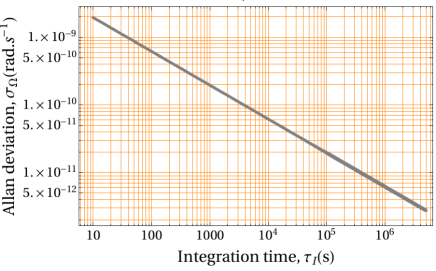
Figure 23: Computed rotation rate in the form of the Allan standard deviation for a projection-noise-limited AI using a circular waveguide.

In fact, in the 1960s, using general relativity, Leonard Schiff predicted that a free-falling inertial frame in a polar orbit around a rotating gravitational source experiences two orthogonal rotations with respect to the fixed inertial frame of the Universe. schiff ; schiff1 These two phenomena, called the geodetic and Lense-Thirring effects, are characterized by rotation rates of 6.6 arcseconds/year and 33 milliarcseconds/year, respectively (1 milliarcsecond = $4.848\times 10^{-9}$ rad s^-1), for an orbit located 642 km from the Earth.

Recently, in 2011, the Gravity Probe B (GP-B) experiment developed by Stanford University and NASA confirmed these predictions with a precision of 1% by using a satellite. The science (data recording) phase of this mission lasted 353 days. GPB ; GPB1 If, in an analogous way, we would like to measure, for instance, the geodetic effect by using cold guided atoms on an atom chip with a precision of 5% in 1 year, then we would need a gyrometer with a stability of about $5.2\times 10^{-14}$ rad s^-1. From the result presented in Fig. 23 and using the parameter values stated above, such a measurement would require 47 years!

However, this problem should be tackled in a different way. The meaningful question is whether we can design a compact atom-chip-based gyrometer by using cold guided atoms to reliably measure the geodetic effect from a satellite orbiting at 642 km above Earth. Part of the answer to this question is presented in Fig. 24, which shows the $v\text{-}2T$ diagram (i.e., interrogation time versus launching speed) with a 5% precision for 12 months of integration time.

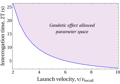
Figure 24: Experimental limits of the launching speed and the AI interrogation time compatible with the observation of the geodetic effect with 5% precision in 12 months of integration.

We learn from Fig. 24 that, if the atoms are launched with, say, an initial velocity of 4$v_{\rm r}$, then we need a minimum interrogation time $2T=9$ s to achieve 5% precision in the measurement. For this particular case, we would need a 37-mm-radius circular magnetic guide.

Suppose now that we can develop an atom chip gyrometer compatible with the CubeSat technology. cubesat In such a scenario, we could foresee, for example, the simultaneous measurement of the geodetic effect using two cubesats orbiting at different distances from Earth. The more distant AI could provide a reference measurement in the common frame of the two satellites, and a differential signal could provide better precision to demonstrate this effect of general relativity. Moreover, if a multi-axis atom-chip-based inertial sensor is developed, then it could be used to realize a drag-free satellite configuration for this scenario. Finally, to have an idea of the potential applications accessible with this AI configuration, Fig. 25 shows the order of magnitude of the rotation rate associated with different fundamental physics phenomena.

Figure 25: Order of magnitude of rotation rates characteristic of different phenomena in geophysics and fundamental physics. These rotation rates are scaled to the rotation rate of Earth: $\Omega_{\rm E}=7.29\times 10^{-5}$ rad s^-1.

An important point to have in mind in the design of a cold atom sensor is the scale of the instrument in terms of volume, power consumption, and weight. For an atom-chip-based sensor, the core of the physics package (i.e., the chip) is a few square centimeters, its power consumption can be kept below 1 W, and, considering the holder, it can weigh up to a few hundred grams. The next important element in the physics package is the vacuum system. By using a glass cell, its volume can be as small as 10 cm³. However, a physics package with such a small vacuum chamber would certainly require a second chamber to realize a double-MOT configuration to avoid reducing the lifetime of the cold samples. In fact, the vacuum system plays a key role in determining the dead time between measurements. Dugrain ; jmm For instance, assume that the interferometer uses molasses cooled atoms. If we use a single vacuum chamber, then the expected dead time is on the order of 5 s. If we use a double-chamber vacuum system (2DMOT + 3DMOT), then the dead time can be reduced to less than 1 s. In both cases, if we use evaporatively cooled atoms, then we need to add, typically, at least 3 s to the previous values. From the reported results (see, for instance, Ref. grosse, ), one can expect that a physics package of 1 L and 1 kg is feasible for this type of sensor.

Another key element of the sensor is the laser source. Today, low-phase-noise transportable laser sources are commercially available. muquans To best exploit the compactness of atom chips, an important technological effort is required to integrate such laser sources onto an atom chip substrate.

Two other important sensor requirements for inertial navigation and guidance are the bandwidth and the dynamic range. High-data-rate sensors are demonstrated in Refs.  rakholia, ; savoie, , and a sensor with relatively large dynamic range was demonstrated in Ref. barret, . These experimental realizations are very encouraging because, given the time required to cool the atoms, inertial sensors using atom interferometry technology have in general a very small bandwidth, typically below 1 Hz. This is a clear drawback if the sensor is expected, for instance, to provide guidance to a carrier. In addition, the performance (sensitivity and stability) of a cold atom inertial sensor is dramatically affected by vibrations. Therefore, one might not expect cold atom sensors to supplant the conventional inertial sensors that are commercially available today (i.e., ring laser gyros, fiber-optic gyros, MEMS accelerometers, and gyroscopes). However, contrary to cold atom inertial sensors, conventional sensors lack the requisite stability for long-term navigation, are not absolute, require calibration, and usually need an external reference signal that is susceptible to jamming. Therefore, as an optimal navigation solution one can foresee the hybridization of cold atom and conventional inertial sensors. lautier

V Outlook and conclusion

This review presents the state-of-the-art results in atom interferometry that are relevant for inertial navigation applications. These results were obtained by using laboratory instruments that, given their volume, are not yet compatible with mobile applications. However, they are undoubtedly relevant to fundamental studies and to define the ultimate performance that can be realized with the compact portable sensors. We also discuss a representative set of portable and compact atom interferometers that have demonstrated an inertial sensitivity. In particular, for rotation sensing, examples are given for two classes of interferometers: free-falling atoms and guided atom interferometers. The latter is considered in detail when using an atom chip as the sensor platform. The enabling technologies and a case study of a sensor design for inertial navigation applications are also presented. Notably, from the computed sensitivity in Fig. 19, the expected angular random walk [$1.1\times 10^{-4}$ ${}^{\circ}{\rm h}^{-1/2}$] after 1 h of integration suggests that a sensor based on the design under consideration would be compliant with strategic-grade inertial navigators.

Projection-noise-limited atom interferometric inertial sensors have now been demonstrated in the free-falling configuration. When dealing with atom chips with relatively low atom number, this result suggests that a possible solution to reach the desired performance is to implement quantum metrology protocols by using squeezed and entangled states. eckert ; caves ; riedel ; reinhard ; leo ; koschorreck In this case, the device sensitivity would scale as $\Delta\Phi_{\rm min}\approx\xi(N)/\sqrt{N}$, where $\xi(N)<1$ defines the degree of atomic noise squeezing. In the context of atom interferometry, these states have been generated in optical dipole traps, appel optical cavities in the QED regime, smith and in optical lattices. gross

VI Acknowledgments

I would like to thank the members of the atom interferometry and inertial sensors team at SYRTE. This work was funded by the Délégation Générale de l’Armement (DGA) through the ANR ASTRIDE program (Contracts ANR-13-ASTR-0031-01, ANR-18-ASMA-0007-01), the Institut Francilien de Recherche sur les Atomes Froids (IFRAF), and the Emergence-UPMC program (Contract A1-MC-JC-2011/220).

References

- (1) N. F. Ramsey. History of Atomic Clocks, J. Res. Nat. Bureau of Standards 88, 301 (1983).
- (2) S. Bize et al. Cold atom clocks and applications, J. Phys. B: At. Mol. Opt. Phys. 38 S449 (2005).
- (3) M. Kasevich and S. Chu. Measurement of the gravitational acceleration of an atom with a light–pulse atom interferometer, Appl. Phys. B 54, 321 (1992).
- (4) A. Peters, K. Y. Chung, and S. Chu. High–precision gravity measurements using atom interferometry, Metrologia 38, 25 (2001).
- (5) A. Peters, K. Y. Chung, and S. Chu. Measurement of gravitational acceleration by dropping atoms, Nature 400, 849 (1999).
- (6) S. Abend, M. Gebbe, M. Gersemann, H. Ahlers, H. Müntinga, E. Giese, N. Gaaloul, C. Schubert, C. Lämmerzahl, W. Ertmer, W. P. Schleich, and E. M. Rasel. Atom-Chip Fountain Gravimeter, Phys. Rev. Lett. 117, 203003 (2016).
- (7) M.-K. Zhou et al. Micro-Gal level gravity measurements with cold atom interferometry, Chinese Phys. B 24, 050401 (2015).
- (8) J. M. McGuirk, G. T. Foster, J. B. Fixler, M. J. Snadden, and M. Kasevich. Sensitive absolute–gravity gradiometry using atom interferometry, Phys. Rev. A 65, 033608 (2002).
- (9) G. Rosi, F. Sorrentino, L. Cacciapuoti, M. Prevedelli, and G. Tino. Precision measurement of the Newtonian gravitational constant using cold atoms, Nature 510, 518 (2014).
- (10) G. Lamporesi, A. Bertoldi, L. Cacciapuoti, M. Prevedelli, and G. M. Tino. Determination of the newtonian gravitational constant using atom interferometry, Phys. Rev. Lett. 100, 050801 (2008).
- (11) F. Riehle, Th. Kisters, A. Witte, J. Helmcke, and Ch. J. Bordé. Optical Ramsey spectroscopy in a rotating frame: Sagnac effect in a matter–wave interferometer, Phys. Rev. Lett. 67, 177 (1991).
- (12) T. L. Gustavson, A. Landragin, and M. A. Kasevich. Rotation sensing with a dual atom–interferometer Sagnac gyroscope, Class. Quantum. Grav. 17 1 (2000).
- (13) T. L. Gustavson, P. Bouyer, and M. A. Kasevich. Precision measurements with an atom interferometer gyroscope, Phys. Rev. Lett. 78 2046 (1997).
- (14) B. Canuel, F. Leduc, D. Holleville, A. Gauguet, J. Fils, A. Virdis, A. Clairon, N. Dimarcq, Ch. J. Borde, and A. Landragin. Six axis inertial sensor using cold–atom interferometry, Phys. Rev. Lett. 97 010402 (2006).
- (15) P. Wang, R.-B. Li, H. Yan, J. Wang, and M.-S. Zhan. Demonstration of a Sagnac–type cold atom interferometer with stimulated Raman transitions, Chin. Phys. Lett. 24, 27 (2007).
- (16) K. S. Hardman, P. J. Everitt, G. D. McDonald, P. Manju, P. B. Wigley, M. A. Sooriyabandara, C. C. N. Kuhn, J. E. Debs, J. D. Close, and N. P. Robins. Simultaneous Precision Gravimetry and Magnetic Gradiometry with a Bose-Einstein Condensate: A High Precision, Quantum Sensor, Phys. Rev. Lett. 117, 138501 (2016).
- (17) QuanS, http://www.muquans.com/
- (18) AOSense, http://aosense.com/
- (19) P. Gillot, O. Francis, A. Landragin, F. Pereira Dos Santos, and S. Merlet. Stability comparison of two absolute gravimeters : optical versus atomic interferometers, Metrologia 51, L15 (2014).
- (20) R. Bouchendira, P. Cladé, S. Guellati-Khélifa, F. Nez, and F. Biraben. New Determination of the Fine Structure Constant and Test of the Quantum Electrodynamics, Phys. Rev. Lett. 106, 080801 (2011).
- (21) D. S. Weiss, B. C. Young, and S. Chu. Precision measurement of based on photon recoil using laser-cooled atoms and atomic interferometry, Appl. Phys. B 59, 217 (1994).
- (22) D. Aguilera et al. STE-QUEST - Test of the Universality of Free Fall Using Cold Atom Interferometry, Classical Quant. Grav. 31, 115010 (2014).
- (23) J. B. Fixler, G. T. Foster, J. M. McGuirk, and M. A. Kasevich. Atom interferometer measurement of the newtonian constant of gravity, Science 315, 74 (2007).
- (24) D. Savoie, M. Altorio, B. Fang, L. A. Sidorenkov, R. Geiger, and A. Landragin. Interleaved Atom Interferometry for High Sensitivity Inertial Measurements, Sci. Adv. 4, eaau7948 (2018).
- (25) R. Geiger, I. Dutta, D. Savoie, B. Fang, C. L. Garrido Alzar, B. Venon, and A. Landragin. Continuous cold atom inertial sensor with 1 nrad.s-1 rotation stability, Proc. SPIE 9900, Quantum Optics, 990005 (2016). doi: 10.1117/12.2228533
- (26) B. Barrett, P.-A. Gominet, E. Cantin, L. Antoni-Micollier, A. Bertoldi, B. Battelier, P. Bouyer, J. Lautier, and A. Landragin, in Atom Interferometry, Proceedings of the International School of Physics Enrico Fermi, Course CLXXXVIII, Varenna, 2013, edited by G. M. Tino and M. A. Kasevich (IOS, Amsterdam, 2014), p. 493.
- (27) A. A. Velikoseltsev, K.-U. Schreiber, A. Yankovsky, J.-P. R. Wells, A. Boronachin, and A. Tkachenko. On the application of fiber optic gyroscopes for detection of seismic rotations, J. Seismol.16, 623 (2012).
- (28) A. A. Velikoseltsev, D. P. Luk’yanov, V.I. Vinogradov, and K.-U. Schreiber. Super-large optical gyroscopes for applications in geodesy and seismology: state-of-the-art and development prospects, Quantum Electronics 44, 1151 (2014).
- (29) L. I. Schiff. Possible New Experimental Test of General Relativity Theory, Phys. Rev. Lett. 4, 215 (1960).
- (30) L. I. Schiff. Motion of a Gyroscope According to Einstein’s Theory of Gravitation, Proc. Natl. Acad. Sci. USA 46, 871 (1960).
- (31) I. Dutta, D. Savoie, B. Fang, B. Venon, C. L. Garrido Alzar, R. Geiger, and A. Landragin. Continuous Cold-Atom Inertial Sensor with 1 nrad/sec Rotation Stability, Phys. Rev. Lett. 116, 183003 (2016).
- (32) M.A. Kasevich, MAGGPI program final report, DTIC, 2008.
- (33) N. Yu, J. M. Kohel, J. R. Kellogg, and L. Maleki. Development of an atom-interferometer gravity gradiometer for gravity measurement from space, Appl. Phys. B 84, 647 (2006).
- (34) T. van Zoest et al. Bose-Einstein Condensation in Microgravity, Science 328, 1540 (2010).
- (35) D. Becker et al. Space-borne Bose-Einstein condensation for precision interferometry, Nature 562, 391 (2018).
- (36) P. Berg, S. Abend, G. Tackmann, C. Schubert, E. Giese, W. P. Schleich, F. A. Narducci, W. Ertmer, and E. M. Rasel. Composite-Light-Pulse Technique for High-Precision Atom Interferometry, Phys. Rev. Lett. 114, 063002 (2015).
- (37) R. Geiger, V. Ménoret, G. Stern, N. Zahzam, P. Cheinet, B. Battelier, A. Villing, F. Moron, M. Lours, Y. Bidel, A. Bresson, A. Landragin, and P. Bouyer. Detecting inertial effects with airborne matter-wave interferometry, Nat. Comm. 2, 474 (2011).
- (38) Z. Jiang, V. Palinkas, F. E. Arias, J. Liard, S. Merlet, H. WilmesL. Vitushkin, L. Robertsson, L. Tisserand, F. Pereira Dos Santos et al. The 8th International Comparison of Absolute Gravimeters 2009: the first Key Comparison (CCM.G-K1) in the field of absolute gravimetry, Metrologia 49, 666 (2012).
- (39) G. Sagnac. L’éther lumineux démontré par l’effet vent relatif d’éther dans un interféromètre en rotation uniforme, Compte rendus de l’Académie des Sciences 95, 708 (1913).
- (40) V. Vali and R. W. Shorthill. Fiber ring interferometer, Appl. Opt. 15, 1099 (1976).
- (41) W. M. Macek and T. M. Davis Jr. Rotation rate sensing with travelling–wave ring lasers, Appl. Phys. Lett. 2, 67 (1963).
- (42) O. Carnal and J. Mlynek. Young’s double slit experiment with atoms: a simple atom interferometer, Phys. Rev. Lett. 66, 2689 (1991).
- (43) F. Shimizu, K. Shimizu, and T. Takuma. Double–slit interference with ultracold metastable neon atoms, Phys. Rev. A 55, R17 (1992).
- (44) D. Keith, C. Ekstrom, Q. Turchette, and D. Pritchard. An interferometer for atoms, Phys. Rev. Lett. 66, 181 (1991).
- (45) Ch. J. Bordé. Atomic interferometry with internal state labelling, Phys. Lett. A 140, 10 (1989).
- (46) A. Tonyushkin and M. Prentiss. Straight macroscopic magnetic guide for cold atom interferometer, J. Appl. Phys. 108, 094904 (2010).
- (47) S. Wu, E. Su, and M. Prentiss. Demonstration of an area-enclosing guided-atom interferometer for rotation sensing, Phys. Rev. Lett. 99, 173201 (2007).
- (48) J. H. T. Burke and C. A. Sackett. Scalable Bose-Einstein-condensate Sagnac interferometer in a linear trap, Phys. Rev. A 80, 061603(R) (2009).
- (49) H. Yan. Guided atom gyroscope on an atom chip with symmetrical state-dependent microwave potentials, Appl. Phys. Lett. 101, 194102 (2012).
- (50) S. Gupta, K. W. Murch, K. L. Moore, T. P. Purdy, and D. M. Stamper-Kurn. Bose-Einstein condensation in a circular waveguide, Phys. Rev. Lett. 95, 143201 (2005).
- (51) J. M. Reeves, O. Garcia, B. Deissler, K. L. Baranowski, K. J. Hughes, and C. A. Sackett. Time-orbiting potential trap for Bose-Einstein condensate interferometry, Phys. Rev. A 72, 051605(R) (2005).
- (52) A. S. Arnold. Adaptable-radius, time-orbiting magnetic ring trap for Bose-Einstein condensates, J. Phys. B: At. Mol. Opt. Phys. 37 L29 (2004).
- (53) M. Gildemeister, E. Nugent, B. E. Sherlock, M. Kubasik, B. T. Sheard, and C. J. Foot. Trapping ultracold atoms in a time-averaged adiabatic potential, Phys. Rev. A 81, 031402(R) (2010).
- (54) I. Lesanovsky and W. von Klitzing. Time-Averaged Adiabatic Potentials: Versatile Matter-Wave Guides and Atom Traps, Phys. Rev. Lett. 99, 083001 (2007).
- (55) S. Pandey, H. Mas, G. Drougakis, P. Thekkeppatt, V. Bolpasi, G. Vasilakis, K. Poulios, and W. von Klitzing. Hypersonic Bose-Einstein condensates in accelerator rings, Nature 570 205 (2019).
- (56) B. E. Sherlock, M. Gildemeister, E. Owen, E. Nugent, and C. J. Foot. Time-averaged adiabatic ring potential for ultracold atoms, Phys. Rev. A 83, 043408 (2011).
- (57) P. F. Griffin, E. Riis, and A. S. Arnold. Smooth inductively coupled ring trap for atoms, Phys. Rev. A 77, 051402(R) (2008).
- (58) A. S. Arnold, C. S. Garvie, and E. Riis. Large magnetic storage ring for Bose-Einstein condensates, Phys. Rev. A 73, 041606(R) (2006).
- (59) O. Morizot, Y. Colombe, V. Lorent, H. Perrin, and B. M. Garraway. Ring trap for ultracold atoms, Phys. Rev. A 74, 023617 (2006).
- (60) W. H. Heathcote, E. Nugent, B. T. Sheard and C. J. Foot. A ring trap for ultracold atoms in an RF-dressed state, New J. Phys. 10, 043012 (2008).
- (61) A. Chakraborty, S. R. Mishra, S. P. Ram, S. K. Tiwari, and H. S. Rawat. A toroidal trap for cold 87Rb atoms using an rf-dressed quadrupole trap, J. Phys. B: At. Mol. Opt. Phys. 49 075304 (2016).
- (62) Y.-J. Chen, A. Hansen, G. W. Hoth, E. Ivanov, B. Pelle, J. Kitching, and E. A. Donley. Single-Source Multiaxis Cold-Atom Interferometer in a Centimeter-Scale Cell, Phys. Rev. Appl. 12, 014019 (2019).
- (63) A. V. Rakholia, H. J. McGuinness, and G. W. Biedermann. Dual-Axis High-Data-Rate Atom Interferometer via Cold Ensemble Exchange, Phys. Rev. Appl. 2, 054012 (2014).
- (64) G. Tackmann, P. Berg, C. Schubert, S. Abend, M. Gilowski, W. Ertmer and E. M. Rasel. Self-alignment of a compact large-area atomic Sagnac interferometer, New J. Phys. 14, 015002 (2012).
- (65) B. Barrett, L. Antoni-Micollier, L. Chichet, B. Battelier, T. Lévèque, A. Landragin, and P. Bouyer. Dual matter-wave inertial sensors in weightlessness, Nat. Comm. 7, 13786 (2016).
- (66) N. M. Barbour. Inertial Navigation Sensors, in Advances in Navigation Sensors and Integration Technology, NATO RTO Lecture Series 232 (RTO/NATO, London, 2004).
- (67) M. Keil et al. Fifteen years of cold matter on the atom chip: promise, realizations, and prospects, J. Mod. Opt. 63, 1840 (2016), and references therein.
- (68) J. Fortagh and C. Zimmermann. Magnetic microtraps for ultracold atoms, Rev. Mod. Phys. 79, 235 (2007).
- (69) R. Folman. Material Science for Quantum Computing with Atom Chips, QIP 10, 995 (2011).
- (70) R. Folman, P. Kruger, J. Schmiedmayer, J. Denschlag, and C. Henkel. Microscopic atom optics: from wires to an atom chip, Adv. Atom Mol. and Opt. Phys. 48, 263 (2002).
- (71) B. Lev. Fabrication of Micro-Magnetic Traps for Cold Neutral Atoms, Quantum Information and Computation 3, 450 (2003).
- (72) Atom Chips, edited by J. Reichel and V. Vuletic (Wiley VCH, Weinheim, 2011).
- (73) G. J. Dick. Local oscillator induced instabilities, Proc. 19th Annual Precise Time and Time Interval (PTTI) Applications and Planning Meeting, 133 (1987).
- (74) G. A. Sinuco-Leon and B. M. Garraway. Addressed qubit manipulation in radio-frequency dressed lattices, New J. Phys. 18, 035009 (2016).
- (75) M. Ammar et al. Symmetric microwave potentials for interferometry with thermal atoms on a chip, Phys. Rev. A 91, 053623 (2015).
- (76) C.L. Garrido Alzar, W. Yan, and A. Landragin. Towards high sensitivity rotation sensing using an atom chip, Research in Optical Sciences, OSA Technical Digest, paper JT2A.10 (2012).
- (77) I. Lesanovsky et al. Adiabatic radio-frequency potentials for the coherent manipulation of matter waves, Phys. Rev. A 73, 033619 (2006).
- (78) T. Fernholz et al. Dynamically controlled toroidal and ring-shaped magnetic traps, Phys. Rev. A 75, 063406 (2007).
- (79) S. J. Kim et al. Controllable asymmetric double well and ring potential on an atom chip, Phys. Rev. A 93, 033612 (2016).
- (80) D. Cassettari, B. Hessmo, R. Folman, T. Maier, and J. Schmiedmayer. Beam splitter for guided atoms, Phys. Rev. Lett. 85, 5483 (2000).
- (81) T. Schumm et al. Matter-wave interferometry in a double well on an atom chip, Nature Phys. 1, 57 (2005).
- (82) K. Maussang, G. E. Marti, T. Schneider, P. Treutlein, Y. Li, A. Sinatra, R. Long, J. Estève, and J. Reichel. Enhanced and reduced atom number fluctuations in a BEC splitter, Phys. Rev. Lett. 105, 080403 (2010).
- (83) Y. Shin, C. Sanner, G.-B. Jo, T. A. Pasquini, M. Saba, W. Ketterle, and D. E. Pritchard. Interference of Bose-Einstein condensates split with an atom chip, Phys. Rev. A 72, 021604(R) (2005).
- (84) Y.-J. Wang, D. Z. Anderson, V. M. Bright, E. A. Cornell, Q. Diot, T. Kishimoto, M. Prentiss, R. A. Saravanan, S. R. Segal, and S. Wu. Atom Michelson interferometer on a chip using a Bose–Einstein condensate, Phys. Rev. Lett. 94, 090405 (2005).
- (85) P. Treutlein, P. Hommelhoff, T. Steinmetz, T. W. Hänsch, and J. Reichel. Coherence in microchip traps, Phys. Rev. Lett. 92, 203005 (2004).
- (86) C. Deutsch, F. Ramirez-Martinez, C. Lacroûte, F. Reinhard, T. Schneider, J. N. Fuchs, F. Piéchon, F. Laloë, J. Reichel, and P. Rosenbusch. Spin self-rephasing and very long coherence times in a trapped atomic ensemble, Phys. Rev. Lett. 105, 020401 (2010).
- (87) L. Qi et al. Magnetically guided Cesium interferometer for inertial sensing, Appl. Phys. Lett. 110, 153502 (2017)
- (88) R. Long, T. Rom, W. Hänsel, T. W. Hänsch, and J. Reichel. Long distance magnetic conveyor for precise positioning of ultracold atoms, Eur. Phys. J. D 35, 125 (2005).
- (89) A. Gn̈ther, M. Kemmler, S. Kraft, C. J. Vale, C. Zimmermann, and J. Fortágh. Combined chips for atom optics, Phys. Rev. A 71, 063619 (2005).
- (90) S. Wu, Y.-J. Wang, Q. Diot, and M. Prentiss. Splitting matter waves using an optimized standing-wave light-pulse sequence, Phys. Rev. A 71, 043602 (2005).
- (91) E. Giese, A. Roura, G. Tackmann, E. M. Rasel, and W. P. Schleich. Double Bragg diffraction: A tool for atom optics, Phys. Rev. A 88, 053608 (2013).
- (92) S. Machluf, Y. Japha, and Ron Folman. Coherent Stern-Gerlach momentum splitting on an atom chip, Nat. Comm. 4, Article: 2424 (2013).
- (93) P. Böhi, M. F. Riedel, J. Hoffrogge, J. Reichel, T. W. Hänsch, and P. Treutlein. Coherent manipulation of Bose-Einstein condensates with state-dependent microwave potentials on an atom chip, Nat. Phys. 5, 592 (2009).
- (94) M. Wilzbach, D. Heine, S. Groth, X. Liu, T. Raub, B. Hessmo, and J. Schmiedmayer. Simple integrated single-atom detector, Opt. Lett. 34, 259 (2009).
- (95) R. Ritter, N. Gruhler, W. Pernice, H. Kübler, T. Pfau, and R. Löw. Atomic vapor spectroscopy in integrated photonic structures, Appl. Phys. Lett. 107, 041101 (2015).
- (96) K. K. Mehta and R. J. Ram. Precise and diffraction-limited waveguide-to-free-space focusing gratings, Sci.Rep. 7, Article: 2019 (2017).
- (97) K. K. Mehta et al. Integrated optical addressing of an ion qubit, Nat. Nano. 11, 1066 (2016).
- (98) M. Kohnen, M. Succo, P. G. Petrov, R. A. Nyman, M. Trupke, and E. A. Hinds. An integrated atom-photon junction, Nat. Phot. 5, 35 (2011).
- (99) W. M. Golding. Quantum modes of atomic waveguides by series techniques, J. Math. Phys. 57, 082107 (2016).
- (100) E. Andersson, T. Calarco, R. Folman, M. Andersson, B. Hessmo, and J. Schmiedmayer. Multimode Interferometer for Guided Matter Waves, Phys. Rev. Lett. 88, 100401 (2002).
- (101) J. H. T. Burke, B. Deissler, K. J. Hughes, and C. A. Sackett. Confinement effects in a guided-wave atom interferometer with millimeter-scale arm separation, Phys. Rev. A 78, 023619 (2008).
- (102) K. K. Das, M. D. Girardeau, and E. M. Wright. Interference of a Thermal Tonks Gas on a Ring, Phys. Rev. Lett. 89, 170404 (2002).
- (103) S. Wu, W. Rooijakkers, P. Striehl, and M. Prentiss. Bidirectional propagation of cold atoms in a “stadium”-shaped magnetic guide, Phys. Rev. A 70, 013409 (2004).
- (104) P. Krüger, L. M. Andersson, S. Wildermuth, S. Hofferberth, E. Haller, S. Aigner, S. Groth, I. Bar-Joseph, and J. Schmiedmayer. Potential roughness near lithographically fabricated atom chips, Phys. Rev. A 76, 063621 (2007).
- (105) B. V. Hall et al. A permanent magnetic film atom chip for Bose–Einstein condensation, J. Phys. B 39, 27 (2006).
- (106) C. D. J. Sinclair et al. Bose-Einstein condensation on a permanent-magnet atom chip, Phys. Rev. A 72, 031603 (2005).
- (107) S. Kraft et al. Anomalous longitudinal magnetic field near the surface of copper conductors, J. Phys. B 35, L469 (2002).
- (108) M. A. Jones et al. Cold atoms probe the magnetic field near a wire, J. Phys. B 37, L15 (2004).
- (109) A. E. Leanhardt et al. Bose-Einstein Condensates near a Microfabricated Surface, Phys. Rev. Lett. 90, 100404 (2003).
- (110) J. Estève et al. Role of wire imperfections in micromagnetic traps for atoms, Phys. Rev. A 70, 043629 (2004).
- (111) D.-W. Wang, M. D. Lukin, and E. Demler. Disordered Bose-Einstein Condensates in Quasi-One-Dimensional Magnetic Microtraps, Phys. Rev. Lett. 92, 076802 (2004).
- (112) L. D. Pietra et al. Cold atoms near surfaces: designing potentials by sculpturing wires, J. Phys.: Conf. Ser. 19, 30 (2005).
- (113) J. Estève et al. Realizing a stable magnetic double-well potential on an atom chip, Eur. Phys. J. D 35, 141 (2005).
- (114) J.-B. Trebbia, C. L. Garrido Alzar, R. Cornelussen, C. I. Westbroock, and I. Bouchoule. Roughness suppression via rapid current modulation on an atom chip, Phys. Rev. Lett. 98, 263201 (2007).
- (115) I. Bouchoule, J.-B. Trebbia, and C. L. Garrido Alzar. Limitations of the modulation method to smooth a wire guide roughness, Phys. Rev. A 77, 023624 (2008).
- (116) V. Dugrain, P. Rosenbusch, and J. Reichel. Alkali vapor pressure modulation on the 100 ms scale in a single-cell vacuum system for cold atom experiments, Rev. Sci. Instruments 85, 083112 (2014).
- (117) S. Kang, K. R. Moore, J. P. McGilligan, R. Mott, A. Mis, C. Roper, E. A. Donley, and J. Kitching. Magneto-optic trap using a reversible, solid-state alkali-metal source, Opt. Lett. 44, 3002 (2019).
- (118) L. Torralbo-Campo, G. D. Bruce, G. Smirne, and D. Cassettari. Light-induced atomic desorption in a compact system for ultracold atoms, Scientific Reports 5, 14729 (2015).
- (119) J. Grosse, S. T. Seidel, D. Becker, M. D. Lachmann, M. Scharringhausen, C. Braxmaier, and E. M. Rasel. Design and qualification of an UHV system for operation on sounding rockets, J. Vac. Sci. Technol. A 34, 031606 (2016).
- (120) D. R. Scherer, D. B. Fenner, and J. M. Hensley. Characterization of alkali metal dispensers and non-evaporable getter pumps in ultrahigh vacuum systems for cold atomic sensors, J. Vac. Sci. Technol. A 30, 061602 (2012).
- (121) A. Basu and L. F. Velásquez-Garcia. An electrostatic ion pump with nanostructured Si field emission electron source and Ti particle collectors for supporting an ultra-high vacuum in miniaturized atom interferometry systems, J. Micromech. Microeng. 26, 124003 (2016).
- (122) J.-M. Martin, S. Bade, W. Dubosclard, M. A. Khan, S. Kim, B. M. Garraway, and C. L. Garrido Alzar. Pumping dynamics of cold-atom experiments in a single vacuum chamber, Phys. Rev. Applied 12, 014033 (2019).
- (123) C. L. Garrido Alzar. Stability analysis of a magnetic waveguide with self-generated offset field, Phys. Rev. A 97, 033405 (2018)
- (124) G.-B. Jo, Y. Shin, S. Will, T. A. Pasquini, M. Saba, W. Ketterle, D. E. Pritchard, M. Vengalattore, and M. Prentiss. Long Phase Coherence Time and Number Squeezing of Two Bose-Einstein Condensates on an Atom Chip, Phys. Rev. Lett. 98, 030407 (2007).
- (125) W. Li, A. K. Tuchman, H.-C. Chien, and M. A. Kasevich. Extended Coherence Time with Atom-Number Squeezed States, Phys. Rev. Lett. 98, 040402 (2007).
- (126) J. A. Stickney, M. B. Squires, J. Scoville, P. Baker, and S. Miller. Collisional decoherence in trapped-atom interferometers that use nondegenerate sources, Phys. Rev. A 79, 013618 (2009).
- (127) M. Horikoshi and K. Nakagawa. Suppression of Dephasing due to a Trapping Potential and Atom-Atom Interactions in a Trapped-Condensate Interferometer, Phys. Rev. Lett. 99, 180401 (2007).
- (128) G. D. McDonald, C. C. N. Kuhn, S. Bennetts, J. E. Debs, K. S. Hardman, M. Johnsson, J. D. Close, and N. P. Robins. 80k momentum separation with Bloch oscillations in an optically guided atom interferometer, Phys. Rev. A 88, 053620 (2013).
- (129) J. E. Debs et al.. Comparing thermal and lasing atomic sources for precision inertial measurement, International Quantum Electronics Conference, IQEC2011 and Conference on Lasers and Electro-Optics, CLEO Pacific Rim 2011, IEEE, Australia, pp. 2082-2084.
- (130) For example, the power dissipated on a gold microwire of m2 cross section fed with 1 A can be as high as 10 W.
- (131) M.-Z. Huang, T. Mazzoni, C. L. Garrido Alzar, and J. Reichel. Towards a quantum-enhanced trapped-atom clock on a chip, Research in Optical Sciences, OSA Technical Digest, paper T5A.32 (2019).
- (132) D. M. Giltner, R. W. McGowan, and S. A. Lee. Atom interferometer based on Bragg scattering from standing light waves, Phys. Rev. Lett. 75, 2638 (1995).
- (133) H. Ahlers et al.. Double Bragg Interferometry, Phys. Rev. Lett. 116, 173601 (2016).
- (134) K. A. Moler, D. S. Weiss, M. Kasevich, and S. Chu. Theoretical analysis of velocity-selective Raman transitions, Phys. Rev. A 45, 342, (1992).
- (135) P. Storey and C. Cohen-Tannoudji. The Feynman path integral approach to atomic interferometry. A tutorial, J. Phys. II France 4 1999, (1994).
- (136) R. Szmuk, V. Dugrain, W. Maineult, J. Reichel, and P. Rosenbusch. Stability of a trapped-atom clock on a chip, Phys. Rev. A 92, 012106 (2015).
- (137) P. Cheinet, B. Canuel, F. Pereira Dos Santos, A. Gauguet, F. Leduc, and A. Landragin. Measurement of the sensitivity function in time-domain atomic interferometer, IEEE Trans. on Instrum. Meas. 57, 1141, (2008).
- (138) D. W. Allan. Time and Frequency (Time Domain) Characterization, Estimation, and Prediction of Precision Clocks and Oscillators, IEEE Transactions on Ultrasonics, Ferroelectrics, and Frequency Control UFFC-34, 647 (1987).
- (139) Such an interrogation time is limited by the lifetime of the magnetic trap. For instance, in the atom chip experiment of Deutsch et al. 5 s were observed in a centimeter-scale glass-cell vacuum chamber deutsch and a 10 s lifetime was demonstrated in a stainless steel vacuum chamber trebbia .
- (140) We have assumed a white noise PSD, in Eq. (IV.3) equals to - cf. Eq. (9).
- (141) C. W. F. Everitt. Gravity Probe B: Final Results of a Space Experiment to Test General Relativity, Phys. Rev. Lett. 106, 221101 (2011).
- (142) https://einstein.stanford.edu/index.html
- (143) http://www.cubesat.org
- (144) J. Lautier, L. Volodimer, T. Hardin, S. Merlet, M. Lours, F. Pereira Dos Santos, and A. Landragin. Hybridizing matter-wave and classical accelerometers, Appl. Phys. Lett. 105, 144102 (2014).
- (145) K. Eckert, P. Hyllus, D. Bruß, U. V. Poulsen, M. Lewenstein, C. Jentsch, T. Müller, E. M. Rasel, and W. Ertmer. Differential atom interferometry beyond the standard quantum limit, Phys. Rev. A 73, 013814 (2006).
- (146) C. M. Caves. Quantum-mechanical noise in an interferometer, Phys. Rev D 23, 1693 (1981).
- (147) M. F. Riedel, P. Böhi, Y. Li, T. W. Hänsch, A. Sinatra, and P. Treutlein. Atom-chip-based generation of entanglement for quantum metrology, Nature 464, 1170 (2010).
- (148) C. L. Degen, F. Reinhard, and P. Cappellaro. Quantum sensing, Rev. Mod. Phys. 89, 035002 (2017).
- (149) L. D. Didomenico, H. Lee, P. Kok, and J. P. Dowling. Quantum interferometric sensors, Proc. of SPIE 5359, Quantum Sensing and Nanophotonic Devices, 169 (2004).
- (150) M. Koschorreck, M. Napolitano, B. Dubost, and M. W. Mitchell. Sub-Projection-Noise Sensitivity in Broadband Atomic Magnetometry, Phys. Rev. Lett. 104, 093602 (2010).
- (151) J. Appel, P. J. Windpassinger, D. Oblak, U. B. Hoff, N. Kjaergaard, and E. S. Polzik. Mesoscopic atomic entanglement for precision measurements beyond the standard quantum limit, Proc. Natl. Acad. Sci. USA 106, 10960 (2009).
- (152) M. H. Schleier-Smith, I. D. Leroux, and V. Vuletic. States of an ensemble of two-level atoms with reduced quantum uncertainty, Phys. Rev. Lett. 104, 073604 (2010).
- (153) C. Gross, T. Zibold, E. Nicklas, J. Esteve and M. K. Oberthaler. Nonlinear atom interferometer surpasses classical precision limit, Nature 464, 1165 (2010).