Pumping dynamics of cold-atom experiments in a single vacuum chamber

Abstract

A nonlinear analytical model for the pressure dynamics in a vacuum chamber, pumped with a sputter ion pump (SIP), is proposed, discussed and experimentally evaluated. The model describes the physics of the pumping mechanism of SIPs in the context of a cold atom experiment. By using this model, we fit pump–down curves of our vacuum system to extract the relevant physical parameters characterizing its pressure dynamics. The aim of this investigation is the optimization of cold atom experiments in terms of reducing the dead time for quantum sensing using atom interferometry. We develop a calibration method to improve the precision in pressure measurements via the ion current in SIPs. Our method is based on a careful analysis of the gas conductance and pumping in order to reliably link the pressure readings at the SIP with the actual pressure in the vacuum (science) chamber. Our results are in agreement with the existence of essentially two pumping regimes determined by the pressure level in the system. In particular we found our results in agreement with the well known fact that for a given applied voltage, at low pressures, the discharge current efficiently sputters pumping material from the pump’s electrodes. This process sets the leading pumping mechanism in this limit. At high pressures, the discharge current drops and the pumping is mainly performed by the already sputtered material.

I Introduction

Quantum sensing plays a significant role in the development of the future quantum technologies reinhard ; leo . So far, this sensing technology has been developed on different physical platforms and, in particular, using cold atoms. Among the most relevant realizations one can count atomic microwave and optical clocks Norman , magnetometers koschorreck ; wildermuth and atom interferometers for inertial sensing canuel ; dutta ; dutta1 ; barret , to mention a few. In fact, their quantum nature offers a very high sensitivity to measure gravity peters ; gillot ; abend , fundamental constants Weiss ; bouchendira , and general relativity effects aguilera ; fixler ; rosi . Nowadays, these experimental realizations have been developed not only to a metrology level, being operated as standards, but also as instruments with a maturity that allows industrial and commercial applications muquans ; aosense .

A key element to reach the required level of sensitivity to a physical phenomenon is the preparation of a well–controlled state of the atoms in terms of their internal and external degrees of freedom. This requires laser cooling in a magneto–optical trap (MOT) to sub–Doppler temperatures (on the order of 1 $\mu$K and below), which unavoidably introduces a dead time in the measurement process. For atom interferometers, this translates into the well known Dick effect that degrades the stability of these devices dick ; giorgio ; quesada ; schioppo . To reduce the MOT loading time, a relatively high background partial pressure of the atoms to be cooled Monroe is required, for example $\sim$10^-8 mbar for ⁸⁷Rb atoms. However, this high background pressure reduces the available lifetime to perform the desired experiments with the trapped atom clouds Bjorkholm and also, it degrades the contrast of the interference fringes leading to a reduction of the signal-to-noise ratio of the measurements.

In a typical cold atom experiment the high background pressure problem is overcome, on the one hand, by using two chambers connected via a differential pumping stage. In this situation, one chamber (at high pressure) is used as a bright source of cold atoms and the other one (at low pressure) as a science chamber. However, this solution is hardly compatible with the realization of cold–atom–based compact and miniature sensors. So, on the other hand, when using a single vacuum chamber incorporating the atom source (i.e. an alkali metal dispenser) after the MOT loading stage the residual background atoms need to be pumped out quickly. This is needed in order to preserve a useful level of lifetime of the trapped atoms and to avoid an important increase of the dead time. This later situation implies the ability to switch from high ($\sim$10^-8 mbar) to low pressure ($\sim$10^-11 mbar) in a few tenths of ms Dugrain . A very promising solution has been recently found kitching which allows one to quickly and reversibly control the Rb background pressure in a cell. In this setup, a MOT with up to 10⁶ atoms has been realized. However, no compatibility with a pressure level of $\sim$10^-11 mbar has been demonstrated yet with this technique.

Besides the investigations presented in Dugrain ; kitching , other relevant studies on the optimized operation of compact ultra–high–vacuum (UHV) systems have been reported before. In campo the authors present a detailed analysis on the use of light–induced atomic desorption to modulate the background pressure of ⁸⁷Rb atoms in a glass cell. They developed a model to find the number of atoms loaded in a MOT when the light is on, and demonstrated an order of magnitude increase under this condition. In the context of atom interferometry and atom sensors, an UHV system was designed and tested for operation in the highly vibrating environment of a rocket grosse . In Ref. scherer the authors investigated the use of passive vacuum pumps (non-evaporable getter pumps) for the development of compact cold atom sensors. Finally, in Ref. basu microfabricated non magnetic ion pumps were demonstrated with the aim of maintaining UHV conditions in miniature vacuum chambers for atom interferometry.

The aim of the present work is to understand from the physics point of view, the pressure dynamics of single vacuum chambers loaded with atoms via a dispenser and pumped out by a SIP. So far, SIPs are commonly used in cold atom experiments requiring UHV. Since they are an unavoidable component, which is at the same time able to provide pressure readings Audi ; Coppa , it is therefore relevant to have a physical model of the observed vacuum dynamics. This dynamics is not only determined by the pumping mechanism of the SIPs but also by conductance of the whole system and the dispenser sourcing effect. Understanding this dynamics would allow, for instance, the design of miniature SIPs basu and avoid the use of pressure gauges improving the compactness of the experiments.

To reach a good fidelity in estimating the pressure at the vacuum chamber, we develop an accurate calibration procedure to quantify the leakage ion current in the SIP. To achieve this goal, we first model the conductance of the vacuum system. Then, using the model and a protocol based on a pulsed dispenser current, we measure the temporal evolution of the pressure in the system. As we will see, the physical parameters describing the pressure dynamics extracted in this way, allow the reduction of the dead time in cold atom experiments by combining a fast loading rate of cold atom clouds (high partial ⁸⁷Rb pressure regime) and a fast removal of background atoms after the production of these clouds Dugrain . It is worth mentioning that the commonly used models SUETSUGU1995105 ; Ho1982 for the SIP pumping speed do not explain the important pressure variations (more than two orders of magnitude) we observed. In fact, on measurement time scales of several minutes the nature of the dominant pumping mechanism changes, and this effect needs to be taken into account.

II Steady state pumping behavior

In this manuscript we will consider a single vacuum chamber system as represented in Fig. 1. It is a simplified configuration containing a chamber of volume $V_{1}$ with the atom source (dispenser) that produces a flow $Q(t)$ that goes to a pump with a nominal pumping speed $S$. The pump and the chamber are connected through a pipe with a conductance $C$. With these definitions, we can then relate the pressure at the chamber $P_{1}(t)$ to the pressure at the pump $P_{2}(t)$. In a steady state, neglecting leaks and in the free molecular regime, these quantities are related by the equation of the steady–state sourcing flux $Q(\infty)$

$$Q(\infty)=C[P_{1}(\infty)-P_{2}(\infty)]=SP_{2}(\infty)=S_{\rm eff}P_{1}(\infty)\ ,$$ (1)

where $S_{\rm eff}$ is the effective pumping speed seen by the chamber as determined by $C$. More generally, $P_{1}$ follows the gas balance equation Chiggiato

$$V_{1}\frac{dP_{1}(t)}{dt}=Q(t)-S_{\rm eff}P_{1}(t)\ .$$ (2)

Since the characteristic pumping time $\tau\equiv V_{1}/S_{\rm eff}$ controls the pressure transients in the vacuum system, $S_{\rm eff}$ needs to be properly determined. This is an important question in particular for cold atom experiments with time dependent sources of alkali atoms.

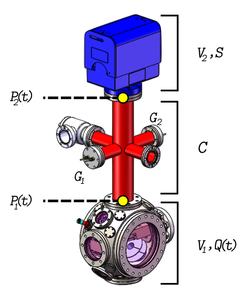
Figure 1: Sketch of the considered experimental setup. The vacuum chamber of volume $V_{1}$ contains the atom source producing a flow $Q(t)$. This gas at a pressure $P_{1}(t)$ in the chamber produces a pressure $P_{2}(t)$ at the pump through a pipe of conductance $C$. In the pump volume $V_{2}$, the atoms are pumped at a nominal speed $S$. Also represented in this figure are deactivated getter pumps $G_{1}$ and $G_{2}$.

II.1 Leakage current

Normally, the pressure is translated into current readings by the pump controller. However, in the presence of alkali gases there exists a modification of the pump leakage current $I_{\ell}$ gammavac . This modification is responsible for an overestimation of the real pressure. It originates from a thin layer of alkali ions stuck to the pump walls. Together with $I_{\ell}$ there is also an ion current $I$ produced by the ionization of the gas flowing through the pump electrodes. These two currents contribute to the measured current $I_{\rm m}$ actually reported by the pump controller (the current reading).

The leakage current $I_{\ell}$ is typically on the order of 100 nA and it is usually neglected in high vacuum regimes (it corresponds to an overestimation of $\simeq$10^-9 mbar). However, neglecting this current affects the use of the ion pump as a pressure gauge in the UHV regime Chiggiato ($<10^{-9}$ mbar). So, we will include the effect of this current in the analysis below.

Following ion pump manufacturers and taking into account that $I=I(P_{2})$ is a function of the pressure at the pump, we have the following expression for $I_{\rm m}$

$$I_{\rm m}(U)=I(P_{2})+I_{\ell}=f(P_{2})\cdot U+I_{\ell}\ ,$$ (3)

where $U$ is the applied voltage between the pump electrodes. From this equation we see that an accurate determination of the actual pressure ($P_{2}$ or $I$) requires a precise knowledge of the leakage current. The usual way of finding $I_{\ell}$ is to measure $I_{\rm m}$ while the pump’s magnets are removed. In this situation, there is no ionization process and we have $I=0$ A. However, this method requires the pump to be stopped and does not allow a real–time monitoring of the pressure.

Here, we measure $I_{\ell}$ by gradually decreasing $U$ within the nominal working range of the pump gammavac . Following Eq. (3), the leakage current is then determined by extrapolating the data to $U=0$ V. The result of this measurement is presented in Fig. 2, where the observed linear behavior indicates that the pressure $P_{2}$ does not depend on the applied voltage $U$ at the pressure levels we performed the experiment.

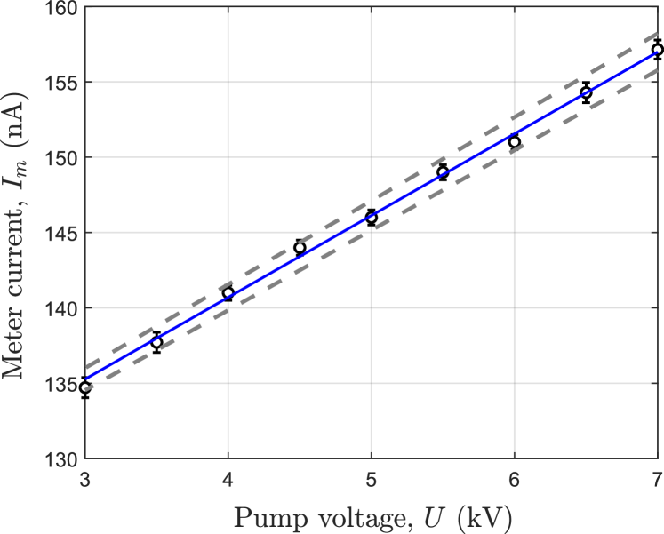
Figure 2: Current-voltage (I–V) characteristic of the pump. The leakage current $I_{\ell}$ = 119.0 $\pm$ 0.4 nA is obtained from a linear fit (solid line) of the measured current $I_{\rm m}$. Dashed lines represent the confidence interval of the fitting parameters.

The obtained value of the leakage current is $I_{\ell}=119.0\pm 0.4$ nA. As we will see in the following section, the accuracy in the pressure measurement obtained with this method allows us to model the pumping dynamics for pressures $<10^{-9}$ mbar.

II.2 Determination of the pressure at the chamber from the SIP current

Once the leakage current is found, we can evaluate the ion current inside the pump $I(P_{2})$ using Eq. (3) and the current reading $I_{\rm m}$. The next problem is then to determine the explicit dependence of the ion current on the pressure at the pump, $f(P_{2})$. Then we can invert the function $f(P_{2})$ and, in the steady state regime, compute the pressure at the chamber using Eq. (1), namely

$$P_{1}=\left(\frac{S}{C}+1\right)P_{2}\ .$$ (4)

In the free molecular regime, the conductance $C$ depends only on the geometry of the vacuum system for a given gas species and temperature. Using the Santeler equation Santeler for the transmission probability through a cylindrical pipe of radius $R$ and length $L$, we can calculate the conductance for a molecule of mass $m$ at room temperature using the relation Chiggiato

$$C=11.75\pi R^{2}\sqrt{\frac{m_{\rm N_{2}}}{m}}\left[1+\frac{3L}{8R}\left(1+\frac{1}{3(1+L/7R)}\right)\right]^{-1}\ .$$ (5)

In Eq. (5) $m_{\rm N_{2}}$ is the mass of a nitrogen molecule, and $R$ and $L$ must be expressed in cm to get $C$ in L.s^-1. Now, let’s get an estimate of the value of $C$ for our vacuum system. In a constant flow regime, the conductance of our particular geometry (central pipe of $L$ = 35.2 cm and $R$ = 3 cm) evaluates to $C=$ 32 L.s^-1 for the ${}^{87}\text{Rb}$ monoatomic gas. This value is obtained neglecting contributions from the cross which is a reasonable assumption in the constant flow regime. Finding $S$ precisely is slightly more difficult when considering pumping of ⁸⁷Rb atoms. However, following the pump’s manufacturer documentation gammavac we can use the linear relation

$$P_{2}=\alpha k\frac{I}{U}\ ,$$ (6)

to express the pressure at the pump in terms of the ion current. Here, $k$=10.9 mbar.V.A^-1 at room temperature and $\alpha$ is a calibration factor. This factor is the ionization vacuum gages’ correction factor which links the pressure measurement of specific gas species to calibration measurements using nitrogen. For Rb $\alpha=4.3$ summers . As we will see later, the empirical relation Eq. (6) does not take into account the fact that the actual relationship between the pressure $P_{2}$ and the ion current in the pump $I$ is nonlinear.

With our MOT, we can realize an independent measurement of $P_{1}$ instead of computing it using Eq. (4). From the loading curve of the MOT, as shown in Fig. 3, we can find $P_{1}$ as indicated in Sackett ; moore . In fact, the loading dynamics of the MOT critically depends on the background pressure of the trapped species and other gases. As has been demonstrated in the past Monroe ; Dugrain ; Sackett ; moore , these curves produce reliable pressure measurements. In our experimental setup we use a mirror MOT obtained with an atom chip. The relevant experimental details are as follows: the red-detuned cooling lasers (-1.5 $\Gamma$ where $\Gamma=2\pi\times$6 MHz is the natural line width of ⁸⁷Rb $D_{2}$ line) have a maximum power of $\simeq$40 mW shared by four independent MOT beams of about 2.5 cm of 1/$e^{2}$ diameter. The magnetic field gradient is 11 G.cm^-1. During 100 s of loading, the fluorescence emitted by the atoms is collected on a photodiode with a solid angle of 1.3$\times 10^{-2}$ srad. This signal is used to compute the atom number. In order to vary the pressure $P_{1}$, we change the dispenser current to produce different stationary gas flows $Q$.

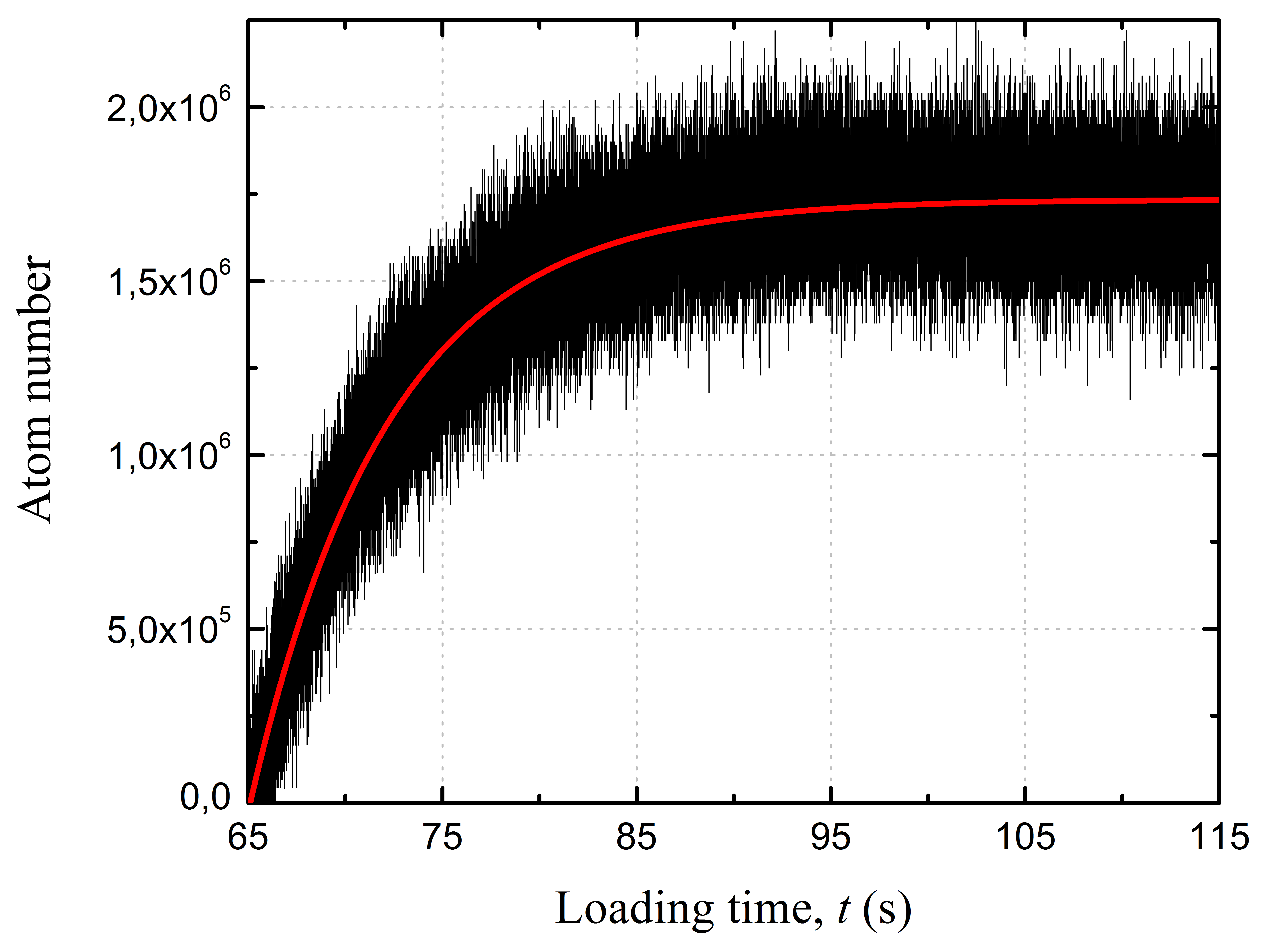
Figure 3: Number of ⁸⁷Rb atoms loaded in the MOT (black) for a dispenser current of 4.75 A. The fit (red solid line) to the experimental data gives a characteristic loading time of $7.13\pm 0.02~{}\text{s}$.

In analogy to Eq. (6), we assume that the ion current $I$ is proportional to the pressure at the vacuum chamber $P_{1}$, measured with the MOT. That is $I=\beta P_{1}$, where $\beta$ is a parameter to be experimentally determined. Then, we can write the following equation for the ion current reading as a function of the pressure $I_{\rm m}$

$$I_{\rm m}=I_{\ell}+\beta P_{1}\ .$$ (7)

In Fig. 4 we plot the dependence of $I_{\rm m}$ on the pressure $P_{1}$ measured from MOT loading curves at steady state. This result offers one independent method to validate the assumption leading to Eq. (7). This method consists in finding the leakage current from MOT measurements and comparing the obtained value with the one extracted from the I–V characterization. Fitting the data in Fig. 4 using Eq. (7), we find for $I_{\ell}$ a value of 130 $\pm$ 20 nA, in good agreement with the result given by the I–V characterization presented in Fig. 2. This agreement supports the use of $\beta$ to compute the pressure in the vacuum chamber by the relation $P_{1}=I/\beta$. For the parameter $\beta$ we obtain the value of (9.2 $\pm$ 0.6)$\times 10^{10}$ nA.mbar^-1.

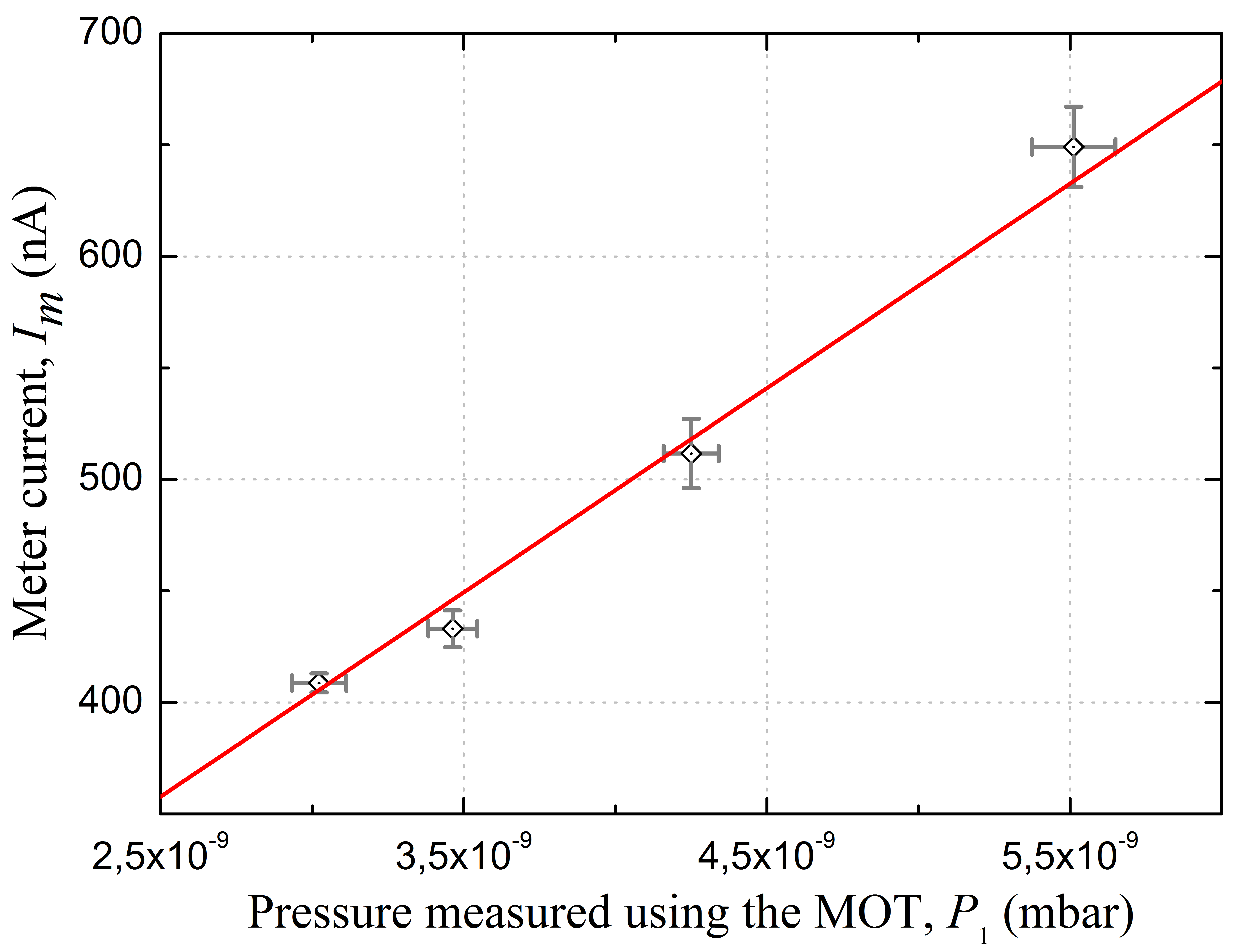
Figure 4: Meter current vs. measured pressure $P_{1}$ from MOT loading curves (points). The leakage current $I_{\ell}$ and the parameter $\beta$ extracted from the fit (solid lined), using Eq. (7), are respectively equal to 130 $\pm$ 20 nA and (9.2 $\pm$ 0.6)$\times 10^{10}$ nA.mbar^-1.

It would be tempting to use the information from equation (4) and Eqs. (6) and (7) to find the pumping speed $S$. However, as we will see in the next section, constant pumping speeds do not properly describe the transient behavior of the pressure when switching on and off the dispenser current.

III Analysis of the nonlinear pumping dynamics

III.1 Derivation of the dynamics

When searching for the reduction of the vacuum system contribution to the dead time between interferometric measurements, we need to focus on the pump–down dynamics that is triggered after loading the MOT and switching off the atom source (dispenser). To achieve this goal, we devised a pressure measurement protocol which is as follows: first, we switch on the dispenser at a given current and monitor the pressure rise until it reaches the steady state moore . The current ranges from 3.75 A to 5 A, with a step of 0.25 A. Then, we switch off the dispenser and record the pressure decay (pump–down curve) until it goes back to the steady state. We allow both of the transient processes to last for about $\simeq$1000 s.

In the following we will develop a mathematical formalism to describe the main physical processes taking place during the pump–down dynamics. Firstly, we will assume that the dispenser is no longer sourcing atoms into the chamber after being switched off. In this case, we can consider that the pressure evolution is mainly due to the pumping by the SIP in the presence of a residual outgassing flow $Q(t)$ coming from the vacuum chamber. In steady state $Q(t)$ will be solely given by the thermal outgassing in the system. Secondly, we will suppose that the pump contains an ensemble of Penning cells with the geometry sketched in Fig. 5. Thirdly, let’s assume that at the time instant $t$:

1. there already exists some sputtered pumping material (e.g. Ti) that pumps the gas, reducing the pressure by an amount $-aP_{2}(t)dt$ [process in Fig. 5];

2. some trapped molecules are released by the incident ion flux increasing the pressure by $cI(t)dt$ [process in Fig. 5];

3. some pumping material sputtered by the ion flux pumps the gas, reducing the pressure by $-aP_{2}(t)\times bI(t)dt$ [process in Fig. 5].

In point 1 above, the coefficient $a$ represents the probability rate at which a particle reaching the cathode (made out of a pumping material) sticks to it. Furthermore, when the gas molecules gets ionized inside the pump [ in Fig. 5], the applied voltage accelerates the ions [ in Fig. 5] towards the cathode. If the ions have sufficient energy they can release previously trapped particles (when they collide with the walls) with a desorption rate proportional to $c$ (point 2) and also, they can sputter pumping material with a yield characterized by the coefficient $b$ (point 3).

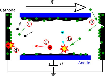
Figure 5: Representation of the pumping unit cell (of Penning type). A high voltage $U$ is applied between the anode (blue), covered by some getter material (black), and the cathode (black). A particle in the gas (green) enters the pumping cell and hits the cathode (a) where it is stuck or deflected towards the anode. On its way to this electrode, the particle collides with an electron (b) and gets ionized. The ion is then accelerated towards the cathode (c) with eventually enough energy to be buried and sputter pumping material (d). The freshly sputtered material covers the internal walls of the cylindrical anode (e) which in then ready to pump more particles.

The physical processes we just described are in agreement with the fact that the pumping speed of the SIP decreases when the pressure decreases. The reason is the decrease of the discharge intensity (current per unit pressure) in this situation. This reduction of the pumping speed depends strongly on the pump parameters such as the applied anode voltage, the magnetic field, and the geometry of the pumping cell.

Collecting together the above mentioned processes, we arrive at the following differential equation for the pressure evolution at the pump

$$\frac{dP_{2}(t)}{dt}=-aP_{2}(t)-aP_{2}(t)\times bI(t)+cI(t)+\frac{Q(t)}{V_{2}}\ ,$$ (8)

where $V_{2}$ is the pump volume. In the next section we use this model to fit the experimental data and determine the physical parameters defining the nonlinear dynamics.

III.2 Practical fitting model

Instead of working directly with the pressure equation (8), here we will derive a practical model that will allow a fitting of the experimental data. Our meter outputs current values and therefore, it would be more natural to work with the ion current $I(t)$ rather than the pressure $P_{2}(t)$. However, the physical processes we just discussed indicate that we cannot use Eq. (6) to relate these quantities. Indeed, $I(t)$ has a nontrivial dependence on the pressure governed by the pressure regime the pump is working in. This fact is encoded by the empirical equation Audi

$$I(t)=hP_{2}(t)^{n}\ ,$$ (9)

where the exponent $n$ is a real number used to identify the different pressure regimes. It depends on the gas species and the geometry of the pump, and will be determined from the fitting procedure. In Eq. (9), $h$ is a time independent calibration parameter defined by the type and size of the pump.

Inserting Eq. (9) into (8) we obtain the following equation in terms of the ion current

$$\frac{dI(t)}{dt}=-\alpha_{1}I(t)-\alpha_{2}I(t)^{2}+\left[\alpha_{3}I(t)+q\right]I(t)^{1-\frac{1}{n}}\ ,$$ (10)

with $\alpha_{1}\equiv na$, $\alpha_{2}\equiv nab$, $\alpha_{3}\equiv nc\sqrt[n]{h}$, $q\equiv n\sqrt[n]{h}Q_{\rm th}/V_{2}$. These parameters will be treated as independent and used in the fitting procedure. When writing (10) we considered that after switching off the dispenser $Q(t)$ reaches the constant thermal outgassing flux $Q_{\rm th}$ in a time scale shorter than the time frame required to reach the steady state. As will we see later, such an approximation is compatible with our observations. We measured the pump–down curves presented in Fig. 6. The points are the experimental data and the solid lines are fits obtained with Eq. (10). As can be seen in this figure, there is a very good agreement between the theory and the experimental data.

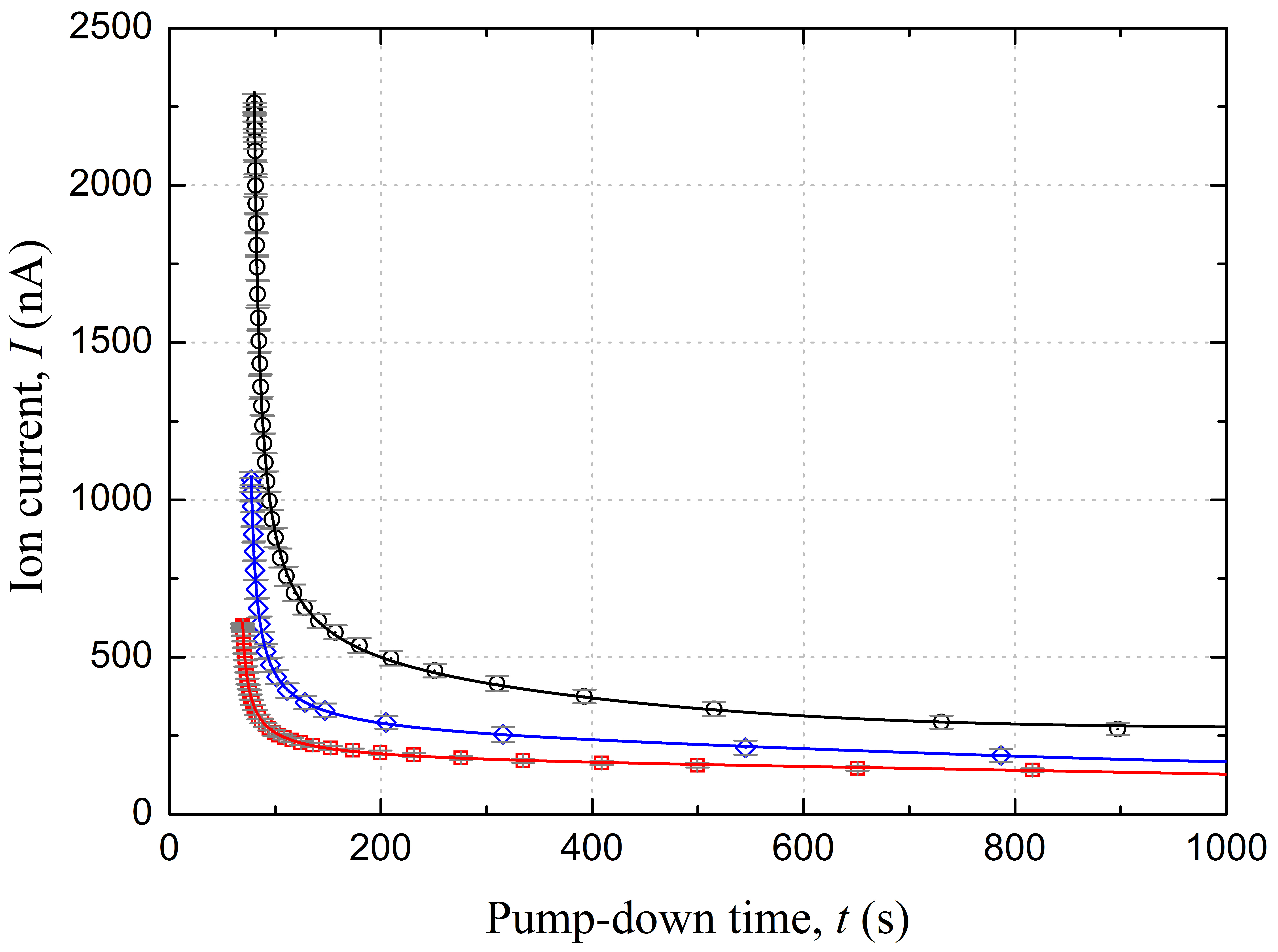
(a)  Dispenser currents: 5 A (black circles), 4.75 A (blue diamonds) and 4.5 A (red squares).

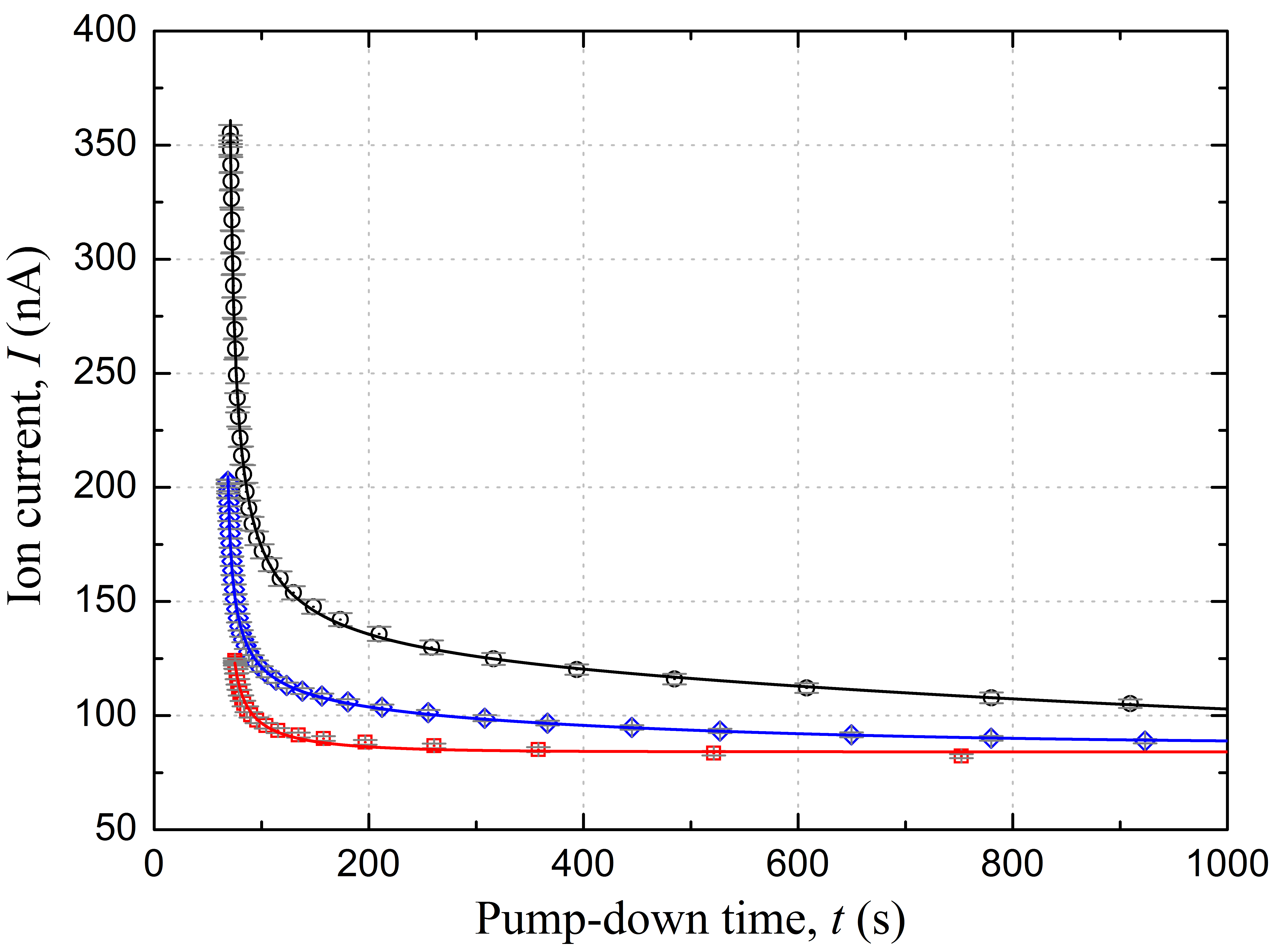
(b)  Dispenser currents: 4.25 A (black circles), 4 A (blue diamonds) and 3.75 A (red squares).

Figure 6: We record the pump–down curves (data points) after switching off the dispenser currents, initially at levels given in captions (a) and (b). In each case, the measured ion current $I(t)$ is fitted (solid lines) by numerical integration of Eq. (10).

To validate the model beyond the criteria set by the fit quality, we study the dependence of the fitting parameters on the pressure $P_{2}$ looking at their behavior in different pressure regimes. The measurement protocol used is as follows: we change the dispenser current and wait until the pressure reaches an equilibrium state. Next, we measure the ion current at this equilibrium situation, before switching off the dispenser. Finally, we start the measurement of the pump–down dynamics. The results obtained with this protocol are presented in Fig. 7. It shows the dependence of the fitting parameters on the initial ion current.

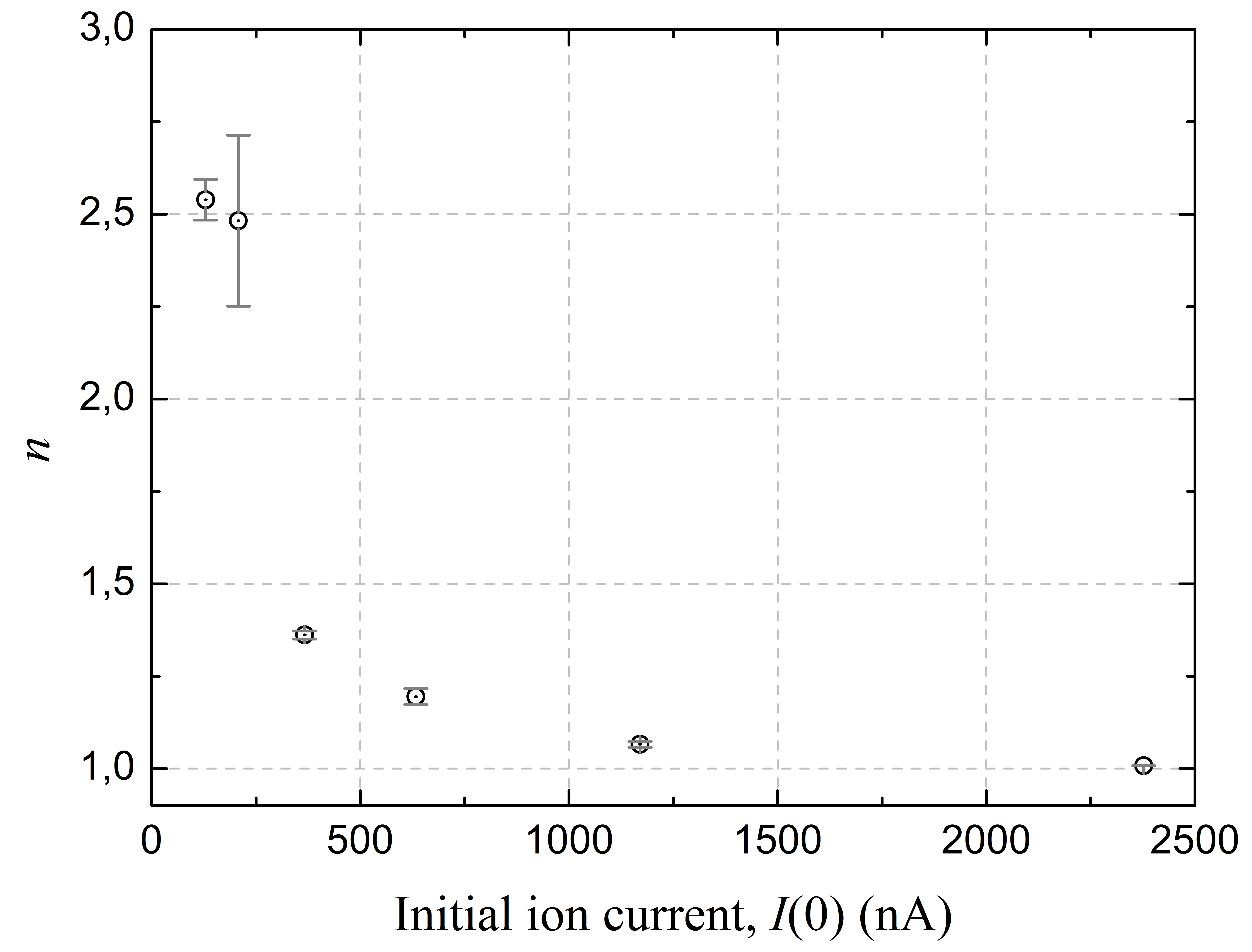
(a)  Pumping regime parameter.

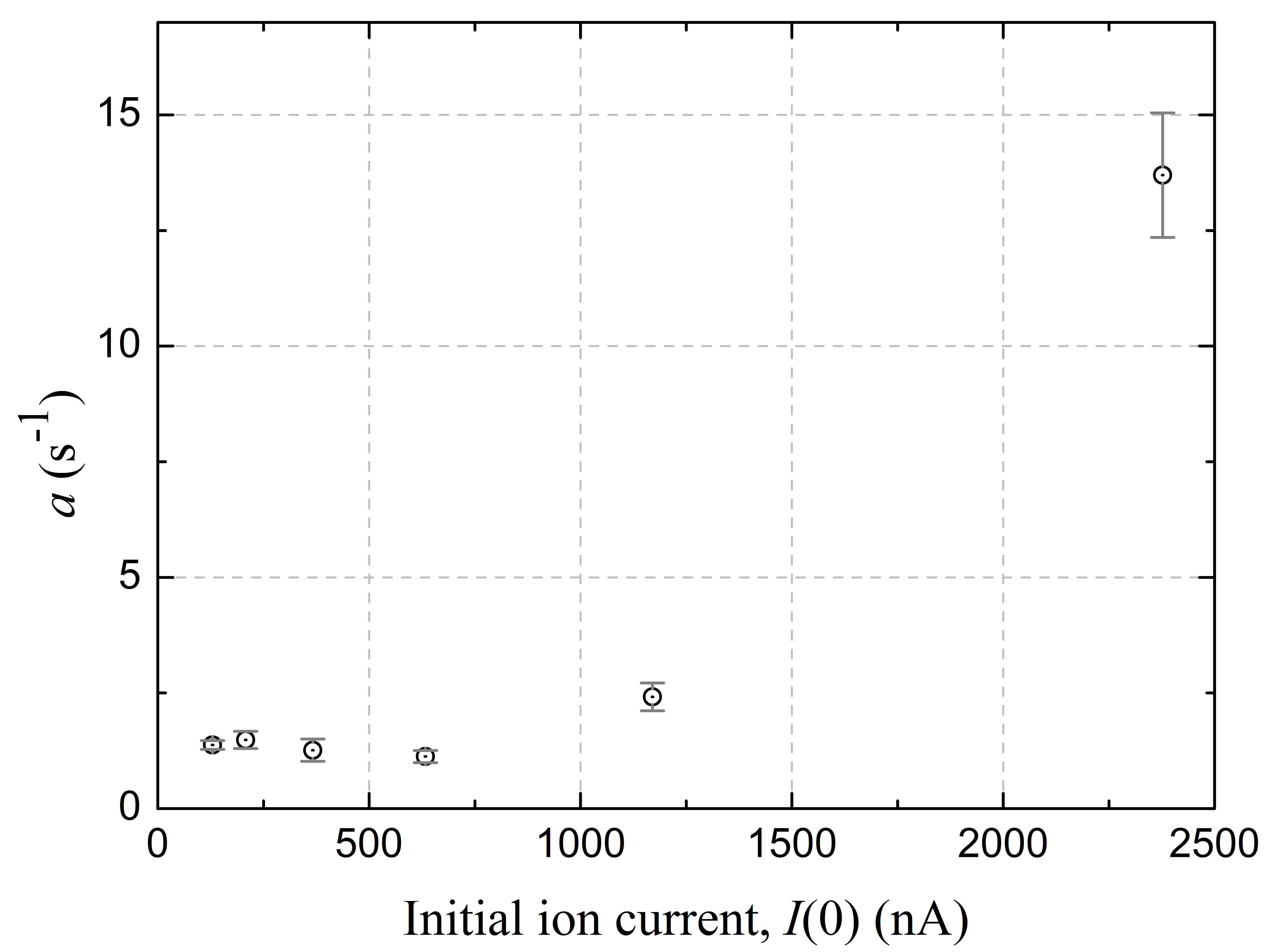
(b)  Former sputtered material pumping rate parameter.

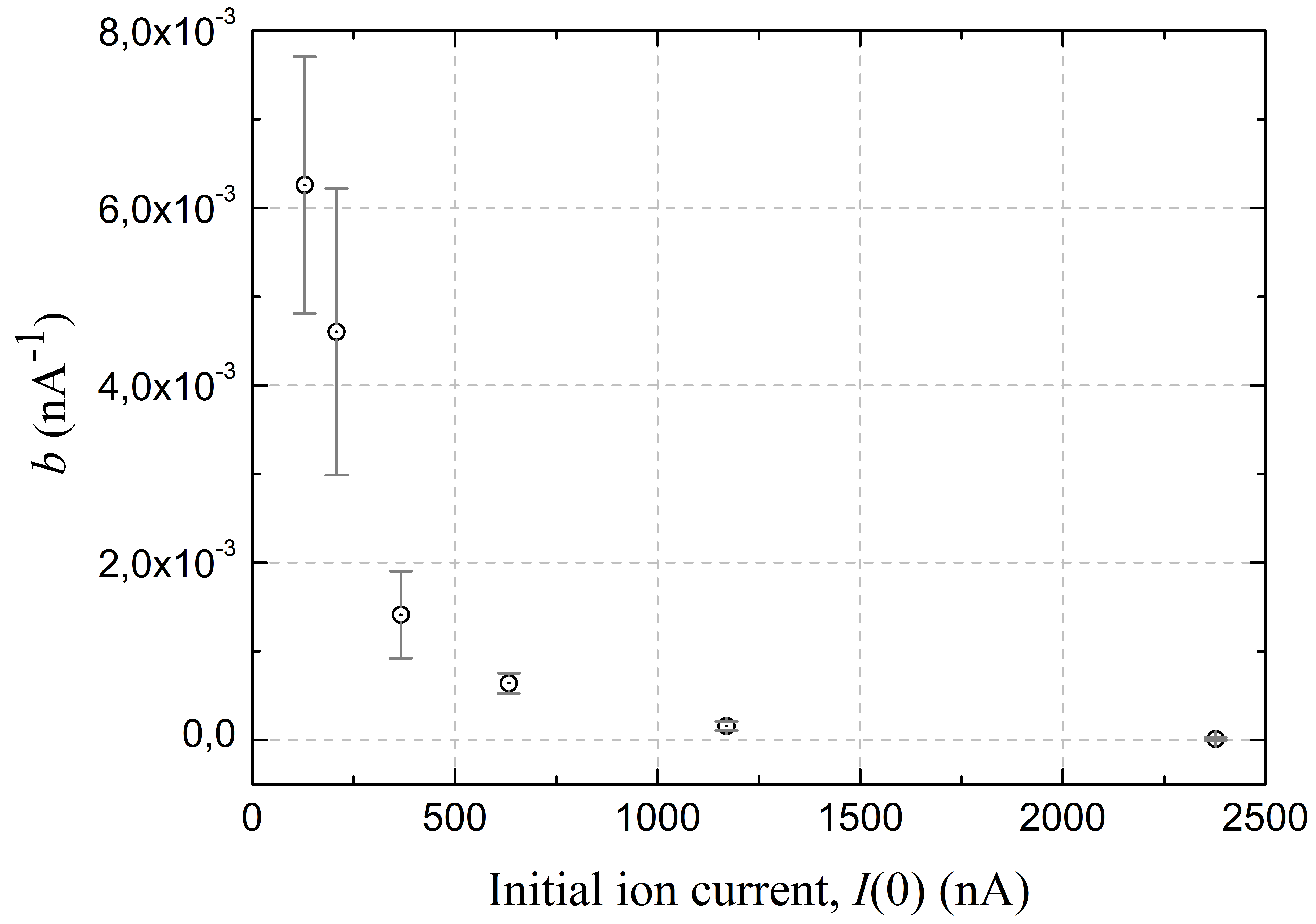
(c)  Instantaneous ion flux induced sputtering pumping rate parameter.

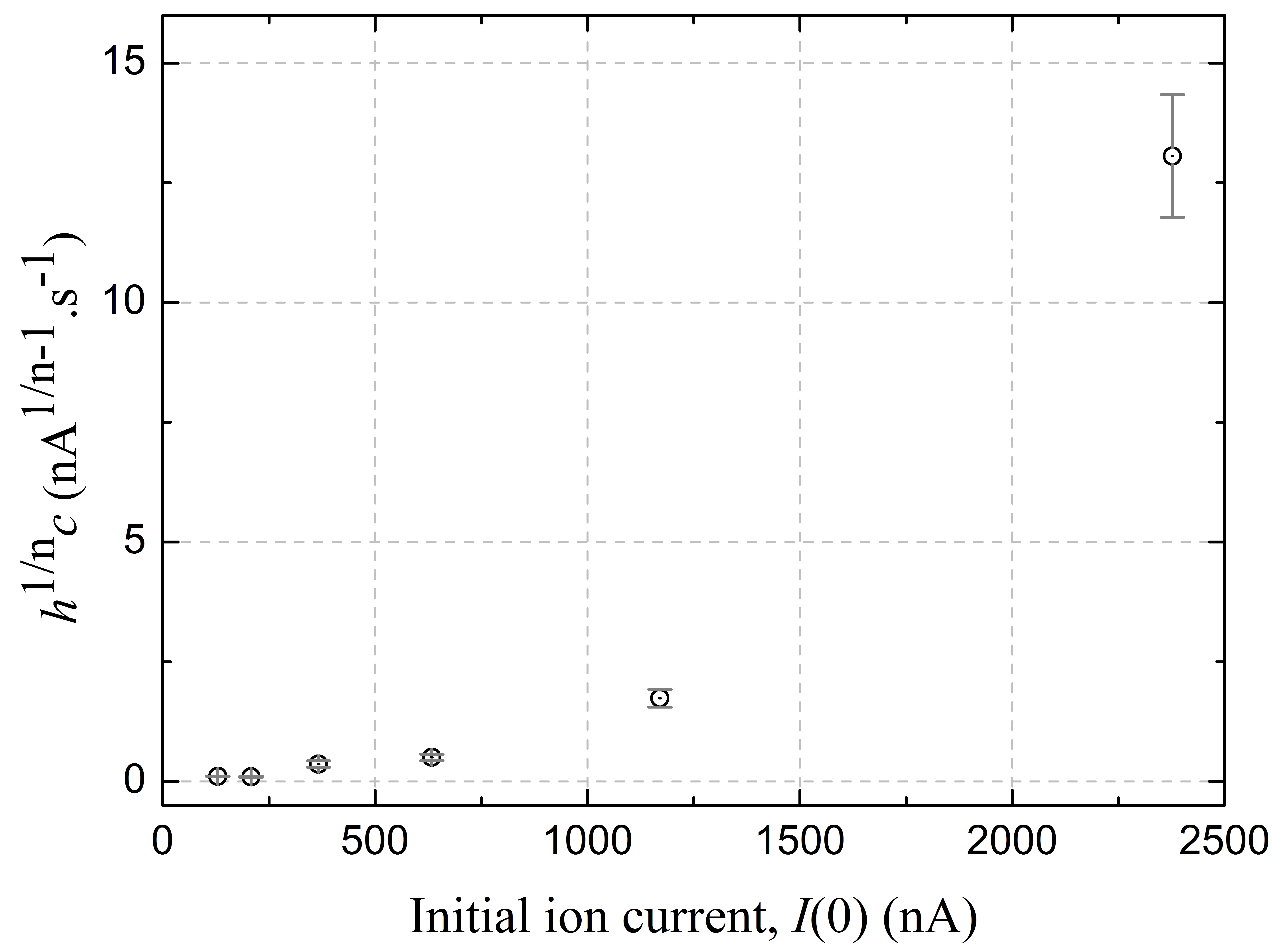
(d)  Ion flux desorption parameter.

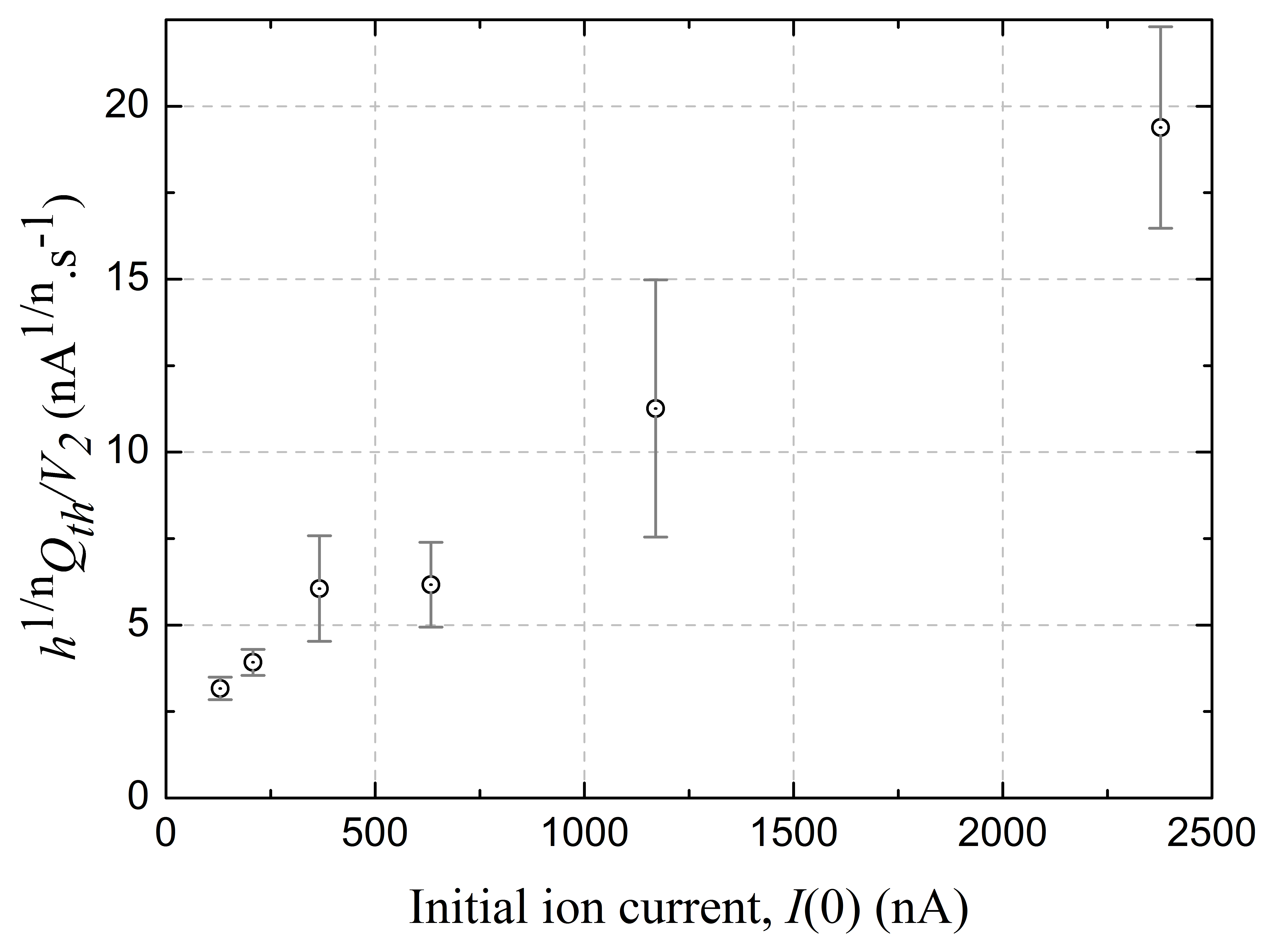
(e)  Thermal outgassing source parameter.

Figure 7: Dependence of the parameters describing the physical processes in the pump volume on the initial ion current (just after turning off the dispenser current). These parameters result from the fitting of the pump–down curves in Fig. 6 using the numerical solution of the differential equation (10).

As expected, the value of $n$ increases when the pressure goes down Dallos1967 as can be seen in Fig. 7(a). Moreover, it reaches unity at the highest measured pressure. The obtained value in this later case is actually compatible with pump manufacturers’ reported values for air. At low pressures it goes beyond 1.5, a value never reported before to our knowledge and that might be in agreement with the fact that we are pumping an alkali gas.

The parameter $a$, according to our model, depends on the pump’s cathode geometry and the sticking factor, this later being a function of the temperature and the gas species. From the measurement in Fig. 7(b) we see that at low initial ion currents (pressures) $a$ is relatively constant. This is expected since in this case the sticking probability should correspond to a linear process given the gas density in the pump. However, when the initial ion current is increased, $a$ eventually increases, suggesting a modification of the sticking probability. This is coherent with the fact that in this situation the behavior of $n$ also indicates a change in the pressure regime. We attributed the change of $a$ with the initial ion current to the change in the sticking probability because the cell geometry does not change.

From Fig. 7(c) we see that the parameter $b$ tends to zero when the initial ion current is increased. This is also an expected behavior since this parameter is related to the discharge current which is depressed by the space–charge effect when the pressure rises. As a consequence, the sputtering rate becomes reduced Audi . In fact, what happens is that at relatively high initial ion currents or pressures, the energy of the ions hitting the cathode is no longer exclusively defined by the applied voltage $U$.

In order to interpret the behavior of the parameters $c$ and $Q_{\rm th}$ we need to isolate them from the calibration factor $h$. This requires us to perform independent measurements. However, it is fair to consider $h$ as a scaling factor in Fig. 7(d) and Fig. 7(e). In this situation the increase of $c$ with the initial ion current might be a consequence of the bombardment boost in the presence of a significant number of gas particles in the pump volume. This process naturally leads to a relatively higher desorption rate of buried molecules. Increasing the initial ion current also leads to an increase in the thermal outgassing flux $Q_{\rm th}$ in the time scale we record the data ($\sim$1000 s). This effect is already observable in Fig. 6 where the steady state ion current value depends on the dispenser current.

Finally, the pressure in the chamber can be determined using the coefficient $\beta$ obtained from the calibration measurement in Fig. 4 and the expression $P_{1}(t)=I(t)/\beta$. This linear relation indicates that the science chamber, at pressure $P_{1}(t)$, acts as a passive particle reservoir feeding the ion current $I(t)$. On the contrary, the Eq. (9) indicates that the pump volume, at a pressure $P_{2}(t)$, can be seen as an active particle reservoir feeding $I(t)$ because of the physical processes involving the gas inside the pump.

Having these ideas in mind, we can outline the next calibration and monitoring protocols for the time evolution of the pressure in the vacuum chamber:

• Calibration protocol

  1. Use the MOT to perform a steady state calibration measurement as in Fig. 4.

  2. From the calibration step 1 and Eq. (7) find $\beta$.

  3. Measure pump–down curves as in Fig. 6 for different initial ion currents $I(0)$.

  4. Using Eq. (10), fit the pump–down curves to find the ion current $I(t)$.

  5. Find the physical parameters of this model for the different $I(0)$ and fit the data in Fig. 7.

• Monitoring protocol

  1. In a given experimental run, and before launching the relevant measurement, find $I(0)$.

  2. Compute the corresponding physical parameters from the fits done on Fig. 7.

  3. Use $\beta$ from step 2 and the solution $I(t)$ from step 4 to compute the pressure in the chamber as $P_{1}(t)=I(t)/\beta$.

IV Conclusion

In this work we have developed a detailed physical model of the nonlinear pressure dynamics in sputter ion pumps. This model has been experimentally corroborated by the measured data. It includes parameters describing the complex physical processes taking place inside the vacuum pump. Moreover, we characterized the system conductance and used pressure measurements with a MOT to establish a link between the pressure in the vacuum chamber and the ion current provided by the pump. From a practical point of view, this relationship allows the pump current to be used as a good indicator of the pressure in the science chamber. From the observed dynamics, we can tailor the effective pumping speed and optimize the MOT loading time with respect to the contradictory requirements of having high repetition rates and high number of atoms in a single chamber. We hope that the physics investigated in this work will be useful in the future to engineer miniature and microscopic scale ion pumps basu for cold atom based compact quantum sensors.

V Acknowledgment

This work has been funded by the Délégation Générale de l’Armement (DGA) through the ANR ASTRID program (contrat ANR-13-ASTR-0031-01), by the UK Defence Science and Technology Laboratory, under Grant No. DSTLX-1000097814 (DSTL–DGA PhD fellowship program), the Institut Francilien de Recherche sur les Atomes Froids (IFRAF), and the Emergence-UPMC program (contrat A1-MC-JC-2011/220). BMG acknowledges the support of the UK Quantum Technology Hub for Sensors and Metrology (UK Engineering and Physical Sciences Research Council grant EP/M013294/1).

References

- (1) C. L. Degen, F. Reinhard, and P. Cappellaro, Quantum sensing, Rev. Mod. Phys. 89, 035002 (2017).
- (2) L. D. Didomenico, H. Lee, P. Kok, and J. P. Dowling, Quantum interferometric sensors, Proc. of SPIE 5359, Quantum Sensing and Nanophotonic Devices, 169 (2004).
- (3) N. F. Ramsey, History of Atomic Clocks, J. Res. Nat. Bureau of Standards 88, 301 (1983).
- (4) M. Koschorreck, M. Napolitano, B. Dubost, and M. W. Mitchell, Sub-Projection-Noise Sensitivity in Broadband Atomic Magnetometry, Phys. Rev. Lett. 104, 093602 (2010).
- (5) S. Wildermuth, S. Hofferberth, I. Lesanovsky, S. Groth, P. Krüger, and J. Schmiedmayer, Sensing electric and magnetic fields with Bose-Einstein condensates, Appl. Phys. Lett. 88, 264103 (2006).
- (6) B. Canuel, F. Leduc, D. Holleville, A. Gauguet, J. Fils, A. Virdis, A. Clairon, N. Dimarcq, Ch. J. Bordé, A. Landragin, and P. Bouyer, Six-axis inertial sensor using cold-atom interferometry, Phys. Rev. Lett. 97, 010402 (2006).
- (7) R. Geiger, I. Dutta, D. Savoie, B. Fang, C. L. Garrido Alzar, B. Venon, and A. Landragin, Continuous cold atom inertial sensor with 1 nrad.s-1 rotation stability, Proc. SPIE 9900, Quantum Optics, 990005 (2016).
- (8) I. Dutta, D. Savoie, B. Fang, B. Venon, C. L. Garrido Alzar, R. Geiger, and A. Landragin, Continuous Cold-Atom Inertial Sensor with 1 nrad/sec Rotation Stability, Phys. Rev. Lett. 116, 183003 (2016).
- (9) B. Barrett, L. Antoni-Micollier, L. Chichet, B. Battelier, T. Lévèque, A. Landragin, and Philippe Bouyer, Dual matter-wave inertial sensors in weightlessness, Nat. Comm. 7, 13786 (2016).
- (10) A. Peters, K. Y. Chung, and S. Chu, Measurement of gravitational acceleration by dropping atoms, Nature 400, 849 (1999).
- (11) P. Gillot, O. Francis, A. Landragin, F. P. D. Santos, and S. Merlet, Stability comparison of two absolute gravimeters: optical versus atomic interferometers, Metrologia 51, L15 (2014).
- (12) S. Abend, M. Gebbe, M. Gersemann, H. Ahlers, H. Müntinga, E. Giese, N. Gaaloul, C. Schubert, C. Lämmerzahl, W. Ertmer, W. P. Schleich, and E. M. Rasel, Atom-Chip Fountain Gravimeter, Phys. Rev. Lett. 117, 203003 (2016).
- (13) R. Bouchendira, P. Cladé, S. Guellati-Khélifa, F. Nez, and F. Biraben, New Determination of the Fine Structure Constant and Test of the Quantum Electrodynamics, Phys. Rev. Lett. 106, 080801 (2011).
- (14) D. S. Weiss, B. C. Young, and S. Chu, Precision measurement of based on photon recoil using laser-cooled atoms and atomic interferometry, Appl. Phys. B 59, 217 (1994).
- (15) D. Aguilera et al., STE-QUEST - Test of the Universality of Free Fall Using Cold Atom Interferometry, Classical Quant. Grav. 31, 115010 (2014).
- (16) J. B. Fixler, G. T. Foster, J. M. McGuirk, and M. A. Kasevich, Atom interferometer measurement of the newtonian constant of gravity, Science 315, 74 (2007).
- (17) G. Rosi, F. Sorrentino, L. Cacciapuoti, M. Prevedelli, and G. Tino, Precision measurement of the Newtonian gravitational constant using cold atoms, Nature 510, 518 (2014).
- (18) QuanS, http://www.muquans.com/
- (19) AOSense, http://aosense.com/
- (20) G. J. Dick, J. D. Prestage, C. A. Greenhall, and L. Maleki, Local Oscillator Induced Degradation of Medium-Term Stability in Passive Atomic Frequency Standards, in Proceedings of the 22nd Annual Precise Time and Time Interval (PTTI) Applications and Planning Meeting, edited by R. L. Sydnor (NASA, Hampton, VA, 1990), pp. 487-508.
- (21) G. Santarelli, C. Audoin, A. Makdissi, P. Laurent, G. J. Dick, and A. Clairon, Frequency stability degradation of an oscillator slaved to a periodically interrogated atomic resonator, IEEE Trans. Ultrason., Ferroelect., Freq. Contr. 45, 887 (1998).
- (22) A. Quesada, R. P. Kovacich, I. Courtillot, A. Clairon, G. Santarelli, and P. Lemonde, The Dick effect for an optical frequency standard, J. Opt. B: Quantum Semiclass. Opt. 5, S150 (2003).
- (23) M. Schioppo, R. C. Brown, W. F. McGrew, N. Hinkley, R. J. Fasano, K. Beloy, T. H. Yoon, G. Milani, D. Nicolodi, J. A. Sherman, N. B. Phillips, C. W. Oates, and A. D. Ludlow, Ultrastable optical clock with two cold-atom ensembles, Nature Photonics 11, 48 (2017).
- (24) C. Monroe, W. Swann, H. Robinson, and C. Wieman, Very cold trapped atoms in a vapor cell, Phys. Rev. Lett. 65, 1571 (1990).
- (25) J. E. Bjorkholm, Collision-limited lifetimes of atom traps, Phys. Rev. A 38, 1599 (1988).
- (26) V. Dugrain, P. Rosenbusch, and J. Reichel, Alkali vapor pressure modulation on the 100 ms scale in a single-cell vacuum system for cold atom experiments, Rev. Sci. Instruments 85, 083112 (2014).
- (27) S. Kang, K. R. Moore, J. P. McGilligan, R. Mott, A. Mis, C. Roper, E. A. Donley, and J. Kitching, Magneto-optic trap using a reversible, solid-state alkali-metal source, Opt. Lett. 44, 3002 (2019).
- (28) L. Torralbo-Campo, G. D. Bruce, G. Smirne, and D. Cassettari, Light-induced atomic desorption in a compact system for ultracold atoms, Scientific Reports 5, 14729 (2015).
- (29) J. Grosse, S. T. Seidel, D. Becker, M. D. Lachmann, M. Scharringhausen, C. Braxmaier, E. M. Rasel, Design and qualification of an UHV system for operation on sounding rockets, J. Vac. Sci. Technol. A 34, 031606 (2016).
- (30) D. R. Scherer, D. B. Fenner, and J. M. Hensley, Characterization of alkali metal dispensers and non-evaporable getter pumps in ultrahigh vacuum systems for cold atomic sensors, J. Vac. Sci. Technol. A 30, 061602 (2012).
- (31) A. Basu and L. F. Velásquez-Garcia, An electrostatic ion pump with nanostructured Si field emission electron source and Ti particle collectors for supporting an ultra-high vacuum in miniaturized atom interferometry systems, J. Micromech. Microeng. 26, 124003 (2016).
- (32) M. Audi and M. de Simon, Ion pumps, Vacuum 37, 629 (1987).
- (33) G. Coppa, A. D’Angola, and R. Mulas, Analysis of electron dynamics in non-ideal Penning traps, Physics of Plasmas 19, 062507 (2012).
- (34) Y. Suetsugu, Numerical calculation of an ion pump’s pumping speed, Vacuum 46, 105, (1995).
- (35) W. Ho, R. K. Wang, T. P. Keng, and K. H. Hu, Calculation of sputtering ion pump speed, J. Vac. Sci. Technol. 20, 1010 (1982).
- (36) P. Chiggiato, Vacuum Technology for Ion Sources, CERN Yellow Report CERN-2013-007, 463 eprint arXiv:1404.0960.
- (37) In this experiment we use the ion pump TiTan 45S-CV from Gamma Vacuum; Technical Bulletin 00.003.971.
- (38) D. J. Santeler, Exit loss in viscous tube flow, J. Vac. Sci. Technol. A 4, 348 (1986).
- (39) R. L. Summers, Empirical Observations on the Sensitivity of Hot Cathode Ionization Type Vacuum Gages, NASA Technical Note D-5285 (1969).
- (40) T. Arpornthip, C. A. Sackett and K. J. Hughes, Vacuum-pressure measurement using a magneto-optical trap, Phys. Rev. A 85, 033420 (2012).
- (41) R. W. G. Moore, L. A. Lee, E. A. Findlay, L. Torralbo-Campo, G. D. Bruce, and D. Cassettari, Measurement of vacuum pressure with a magneto-optical trap: A pressure-rise method, Rev. Sci. Instrum. 86, 093108 (2015).
- (42) A. Dallos and F. Steinrisser, Pumping speeds of getter-ion pumps at low pressures, J. Vacuum Science and Technology 4, 6 (1967).