Stability analysis of a magnetic waveguide with self-generated offset field

Résumé

The unexpected emerging stability of a time-modulated magnetic guide, realized without external offset fields, is demonstrated. We found a steady periodic solution around which the nonlinear dynamics is linearized. To investigate the orbital stability of the guiding, a formal criterion based on the analysis of the eigenvalues of the monodromy matrix of the system dynamics is used. To circumvent the difficulty in finding an analytical expression for these eigenvalues, a Lyapunov transformation of the system variables is proposed. From this transformation an equation of state for the system parameters is derived, and it allows to estimate an upper bound for the computed stability domains. In particular, we found a general expression for the threshold modulation frequency below which the guiding is unstable. Using experimentally accessible parameters, the stable guiding of ⁸⁷Rb atoms is investigated.

The actual technological progress allows the miniaturization of sensors to a level where the laws of the quantum world control the working principles of these devices. Among the outstanding realizations we can cite the SQUID magnetometers squid , the electrical resistance standard based on the quantum Hall effect qhe , and the superconducting gravimeter igrav . In the last decades important efforts have been carried out for the application of matter wave interferometers which belong to another class of quantum devices using cold neutral atoms muquans ; aosense ; gillot ; canuel . In this sense, when the development of compact matter wave interferometers is considered, atom chips come up as a promising technology for the manipulation of cold atoms using complicated geometries keil . Indeed, it is possible to microfabricate on an atom chip a complex wire pattern to create miniature magnetic potentials with the shape required by the targeted application. We can, for example, design arrays of potential wells for quantum information processing sinuco ; wang ; leung , traps for acceleration measurements ammar , and toroidal waveguides for rotation sensing clga ; lesanovsky ; fernholz ; seungjin .

So far all the classical realizations of magnetic potentials, in free space or on atom chips, use a homogeneous offset magnetic field to lift the degeneracy between the confined and not confined atomic states. Generally, a pair of macroscopic coils in a Helmholtz configuration is used to achieve this goal. However, this method is neither practical for the development of a compact device nor compatible with miniature magnetic potentials of complex shapes.

In particular, for a ring guiding potential of a rotation sensor, the use of coils is the simplest and straightforward way to obtain the offset field that fits the symmetry of the potential. However, the switching time of the potential in this situation is undesirably increased limiting the device operation. In fact, the use of coils runs against the realization of high bandwidth and low power consumption sensors, two key performance ingredients for embedded applications such as inertial navigation. This extra timing, added to the already important time required to prepare the samples between each interferometric measurement, will degrade the stability via the Dick effect dick .

Here, a solution to generate the offset field of a magnetic toroidal waveguide that takes into account the above mentioned problems is proposed. The considered magnetic waveguide is generated by three concentric microwires fabricated on an atom chip. The currents in the inner $I_{2}$ and outer $I_{3}$ microwires will be assumed to flow in the same direction, and opposite to the current $I_{1}$ in the central microwire. This currents will be modulated at a frequency $\omega$, as in the configuration used to suppress the magnetic potential roughness (see Fig. 1 in trebbia ). However, instead of setting and trying to keep an exact phase difference of $\pi$ between the currents $I_{2}=I_{3}$ and $I_{1}$, here an small phase offset $\phi\ll\pi$ is introduced so that the total phase difference is $\pi+\phi:$ $I_{1}(t)=A_{1}\cos(\omega t)$ and $I_{2}(t)=I_{3}(t)=A_{2}\cos(\omega t+\pi+\phi)$.

The existence of $\phi$ has two main consequences on the magnetic guiding potential. The first one is the presence of a residual roughness trebbia ; bouchoule that could affect the propagation of atoms close to the surface. This question is beyond the scope of the present work and will be analyzed in detail elsewhere. Nevertheless, this is not a limiting factor for the proposed solution because we can always find a minimum working distance from the atom chip surface where the effects of the roughness on the propagation are totally negligible (see, for example, Fig. 63 in fortagh ). This distance is typically on the order of a few hundreds of microns in the atom chip experiments dealing with matter wave interferometry. The proposed guide with self-generated offset field is also compatible with these working distances. The second consequence is that the obtained time-varying magnetic potential has a dynamical minimum with zero field that goes through the initial atom cloud location, and this fact raises the question about the non-intuitive and unexpected emerging stability of this waveguide against atom losses, to be demonstrated below.

In this paper, an attempt to approach the analytical answer to this stability question is presented. To simplify the mathematical treatment without loss of generality, we will consider a linear section of a ring magnetic guide with a radius much larger than the microwires separation $l$, as shown in Fig. 1. Let us assume that the currents flow in the $y$ direction of a local reference frame, centered at the field minimum (red point in the field lines map above the central wire), for $\phi=0$ and $t=0$, in the $z$ direction perpendicular to the chip surface.

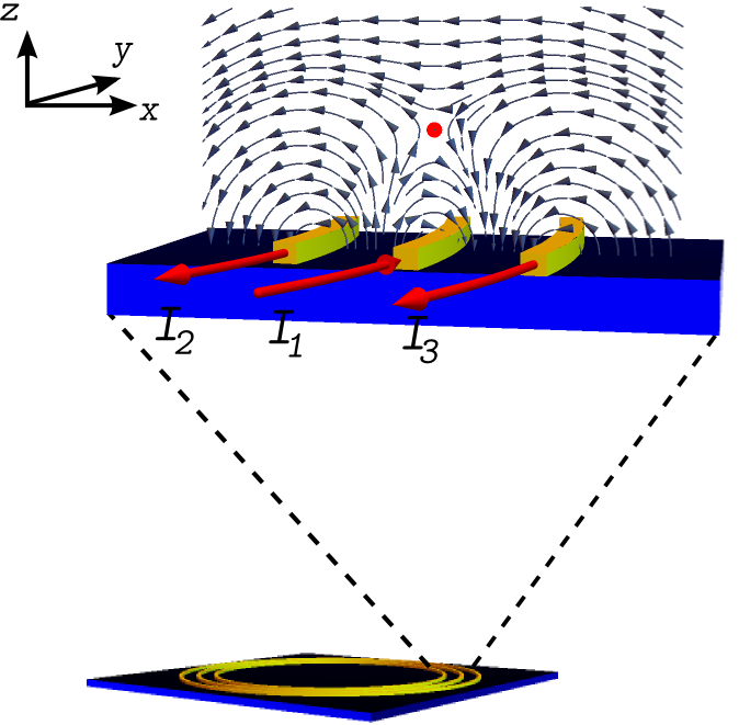
Figure 1: (color online). Current configuration generating the magnetic guide. In the zoom, the considered linear section of the circular guide is represented together with the magnetic field lines map created by the currents. The red point in this map indicates the guide minimum at a given time instant.

Then the dynamics of the atoms in the $x-z$ plane is described by the equations gov1 ; gov ; franzosi

$$M\frac{d^{2}x}{dt^{2}} =\mu\frac{\partial}{\partial x}[\mathbf{n}\cdot\mathbf{B}(\mathbf{r},t)]\ ,$$ (1)

$$M\frac{d^{2}z}{dt^{2}} =\mu\frac{\partial}{\partial z}[\mathbf{n}\cdot\mathbf{B}(\mathbf{r},t)]\ ,$$ (2)

$$\hbar\frac{d\mathbf{n}}{dt} =\mu\mathbf{n}\times\mathbf{B}(\mathbf{r},t)\ ,$$ (3)

where $M$, $\mu$ and $\mathbf{n}$ are the mass of an atom, its magnetic moment and a unit vector in the direction of the magnetic moment, respectively. The magnetic field produced by the microwires $\mathbf{B}(\mathbf{r},t)$ can be written to first order in the position coordinates, and for $\phi\ll\pi$, as fortagh

$$\mathbf{B}(\mathbf{r},t)=[bz\cos(\omega t)+\phi B_{\rm b}\sin(\omega t)]\mathbf{i}+bx\cos(\omega t)\mathbf{k}\ ,$$ (4)

where $B_{\rm b}$ is the magnetic field produced by the inner and outer microwires only, and $b$ is the field gradient. Introducing the dimensionless positions and velocities $X\equiv x/l$, $Z\equiv z/l$, $\tau\equiv\omega t$, $V_{x}\equiv v_{x}/l\omega$, and $V_{z}\equiv v_{z}/l\omega$, the time evolution of the external and internal degrees of freedom of an atom in the magnetic guide with self-generated offset field can be described by the expressions

$$\ddot{X} =-\alpha_{1}n_{z}\cos(\tau)\ ,$$

$$\ddot{Z} =-\alpha_{1}n_{x}\cos(\tau)\ ,$$

$$\dot{n}_{x} =-\alpha_{2}n_{y}X\cos(\tau)\ ,$$ (5)

$$\dot{n}_{y} =-\alpha_{2}[n_{z}Z-n_{x}X]\cos(\tau)-\alpha_{3}n_{z}\sin(\tau)\ ,$$

$$\dot{n}_{z} =\alpha_{2}n_{y}Z\cos(\tau)+\alpha_{3}n_{y}\sin(\tau)\ ,$$

where for simplicity we have omitted the time dependence of the system’s variables. In these equations ${\bf n(\tau)}=(n_{x},n_{y},n_{z})$ will give the instantaneous direction of the atom’s magnetic moment and the dimensionless constants $\alpha_{i}$ are defined by the equations

$$\alpha_{1}\equiv\frac{g_{F}\mu_{B}b}{M\omega^{2}l} =\frac{\omega_{\perp}^{2}}{\omega^{2}}\ ,\ \alpha_{2}\equiv\frac{g_{F}\mu_{B}bl}{\hbar\omega}=\frac{\Omega}{\omega}\ ,$$

$$\alpha_{3}\equiv \frac{g_{F}\mu_{B}\phi B_{\rm b}}{\hbar\omega}=\frac{\omega_{L}}{\omega}\ ,$$ (6)

where $g_{F}$ and $\mu_{B}$ are respectively the Landé factor and the Bohr’s magneton. In the quantum mechanical situation, we need to consider Eqs. (6) describing the atoms with the total angular momentum $\mathbf{F}$ and magnetic moment $\mu=-g_{F}\mu_{B}\mathbf{F}/\hbar$.

Together with the definitions of the $\alpha_{i}$ parameters we also introduced the three characteristic frequencies that determine the different time scales involved in this dynamics: the Larmor frequency of the atoms in the field produced by the two external microwires, $\omega_{L}\equiv g_{F}\mu_{B}\phi B_{\rm b}/\hbar$; the characteristic frequency of the atomic transverse motion, $\omega_{\perp}\equiv\sqrt{g_{F}\mu_{B}b/Ml}$; and the characteristic Rabi frequency at which the magnetic moment couples to the modulated field gradient, $\Omega\equiv g_{F}\mu_{B}bl/\hbar$. Using these characteristic frequencies, the solutions expressed in terms of the $\alpha$’s can be applied to any magnetically trappable atomic species.

The Eqs. (5) represent a system of nonlinear differential equations (NDEs). As usually, we will start the analysis of its stability by linearizing it around a steady periodic solution or orbit. Indeed, it turns out that some properties of the linearized system are also valid for the original nonlinear system, in particular the stability. Thus, we shall seek for periodic solutions in the form

$$X(\tau) \equiv X_{c}(\tau)\cos(\tau)+X_{s}(\tau)\sin(\tau)\ ,$$ (7)

$$Z(\tau) \equiv Z_{c}(\tau)\cos(\tau)+Z_{s}(\tau)\sin(\tau)\ ,$$ (8)

based on the fact that we have harmonic driving of the system’s variables. In Eqs. (7) and (8) the envelopes $X_{c}(\tau),X_{s}(\tau),Z_{c}(\tau),Z_{s}(\tau)$ are supposed to be slowly varying when compared to $\sin(\tau)$ and $\cos(\tau)$. In addition, since by definition at any time we must have ${\bf n}^{2}(\tau)=1$, we will assume the following form for the components of this unit vector

$$n_{x}(\tau) =\cos[\theta(\tau)]\sin[\nu(\tau)]\ ,$$ (9)

$$n_{y}(\tau) =\sin[\theta(\tau)]\sin[\nu(\tau)]\ ,$$ (10)

$$n_{z}(\tau) =\cos[\nu(\tau)]\ .$$ (11)

Substituting Eqs. (7)-(11) in Eqs. (5), neglecting high order derivatives of the slowly varying envelopes, and equating the coefficients in front of the $\sin(\tau)$ and $\cos(\tau)$ terms in the RHS and LHS of the position equations, we arrive finally at the following system of first order NDEs

$$\dot{X_{c}} =-\frac{1}{2}X_{s}\ ,$$

$$\dot{X_{s}} =\frac{1}{2}X_{c}-\frac{\alpha_{1}}{2}\cos(\nu)\ ,$$

$$\dot{Z_{c}} =-\frac{1}{2}Z_{s}\ ,$$

$$\dot{Z_{s}} =\frac{1}{2}Z_{c}-\frac{\alpha_{1}}{2}\cos(\theta)\sin(\nu)\ ,$$ (12)

$$\dot{\theta} =-\cos(\theta)\cot(\nu)\{\alpha_{2}[Z_{c}\cos^{2}(\tau)+Z_{s}\sin(\tau)\cos(\tau)]$$

$$+\alpha_{3}\sin(\tau)\}+\alpha_{2}[X_{c}\cos^{2}(\tau)+X_{s}\sin(\tau)\cos(\tau)]\ ,$$

$$\dot{\nu} =-\sin(\theta)\{\alpha_{2}[Z_{c}\cos^{2}(\tau)+Z_{s}\sin(\tau)\cos(\tau)]$$

$$+\alpha_{3}\sin(\tau)\}\ .$$

It is no difficult to find the steady periodic solutions of equations (12) which are given by $\theta_{k}=k\pi$, $\nu_{m}=(2m+1)\pi/2$, $X_{c}=X_{s}=Z_{s}=0$, and $Z_{c}=(-1)^{k+m}\alpha_{1}$ with $k$ and $m$ integers. If we linearize Eqs. (12) around this steady orbit, then we obtain the following matrix of time varying coefficients to describe the linearized dynamics

$$A(\tau)=\left(\begin{array}[]{cccccc}0&-1/2&0&0&0&0\\ 1/2&0&0&0&0&(-1)^{m}\alpha_{1}/2\\ 0&0&0&-1/2&0&0\\ 0&0&1/2&0&0&0\\ \alpha_{2}\cos^{2}(\tau)&\alpha_{2}\sin(\tau)\cos(\tau)&0&0&0&f(\alpha_{1},\alpha_{2},\alpha_{3},\tau)\\ 0&0&0&0&-f(\alpha_{1},\alpha_{2},\alpha_{3},\tau)&0\end{array}\right)\ ,$$ (13)

with

$$f(\alpha_{1},\alpha_{2},\alpha_{3},\tau)\equiv(-1)^{k}[(-1)^{k+m}\alpha_{1}\alpha_{2}\cos^{2}(\tau)+\alpha_{3}\sin(\tau)]\ .$$ (14)

Now, let us introduce the formal mathematical framework for the analysis of the qualitative behavior of the linearized system. Because of the harmonic terms appearing in Eqs. (5) and (13), and because of the periodic solutions we are interested in, here we are concerned with the orbital stability as defined by Theorem 7.4 in verhulst . In addition, the matrix $A(\tau)$ is continuous $2\pi$-periodic and consequently, by virtue of the Floquet theorem the fundamental matrix $\Phi(\tau)$ of $A(\tau)$ can be written as a product of two matrices and it satisfies the equation lukes

$$\Phi(\tau+2\pi)=\Phi(\tau)\mathcal{M}\ .$$ (15)

The matrix $\mathcal{M}$ is called the monodromy matrix (or Floquet multipliers matrix) and its eigenvalues determine the stability behavior of (12). Indeed, a necessary and sufficient condition for orbital stability of the periodic solution is that all eigenvalues of $\mathcal{M}$ have modulus smaller than 1. This is the criterion that will be used to investigate the stability by linearization of our system of NDEs.

If $\Phi(\tau)$ is a fundamental matrix solution with $\Phi(0)=I$, being $I$ the identity matrix, then we can find $\mathcal{M}$ and its eigenvalues from Eq. (15). Unfortunately, the matrix $A(\tau)$ is not commutative on $[0,+\infty)$ and hence it is not possible to easily find a closed form for $\Phi(\tau)$ that can give some insights on the physics and the underlying structure of the periodic solution. Still, an approximated solution can be found using a Péano-Baker series as given by the Lemma 2.1 in peano , namely

$$\Phi(\tau)=I+\int^{\tau}_{0}dt_{1}A(t_{1})+\int^{\tau}_{0}dt_{1}A(t_{1})\int^{t_{1}}_{0}dt_{2}A(t_{2})$$

$$+\int^{\tau}_{0}dt_{1}A(t_{1})\int^{t_{1}}_{0}dt_{2}A(t_{2})\int^{t_{2}}_{0}dt_{3}A(t_{3})+\cdots\ .$$ (16)

The above presented formalism is summarized in the following algorithm used to check the stability of our magnetic waveguide with self-generated offset field:
Step 1: Find the steady periodic solution of Eqs. (12) and linearize this system around this orbit.
Step 2: Using the matrix $A(\tau)$ resulting from Step 1, compute the fundamental matrix solution from Eq. (16).
Step 3: For a given point in the parameter space $\{\alpha_{1},\alpha_{2},\alpha_{3}\}$, compute the monodromy matrix $\mathcal{M}$ using (15).
Step 4: Find the eigenvalues of $\mathcal{M}$ for the parameter values chosen in Step 3. If all these eigenvalues are smaller than 1 in modulus, then the system is orbitally stable in this point; otherwise, it is not.

Notice that this algorithm is based only on the analysis of the structure of NDEs and thus, it is general and can be applied to any matrix $A(\tau)$. As an example, let us investigate the guiding of ⁸⁷Rb atoms, trapped initially in the $|F=1,m_{F}=2\rangle$ state, in a magnetic guide with a self-generated offset field produced by three microwires separated by $l=15\ \mu$m, with $B_{\rm b}\approx$ 1.5 G and $b\approx$ 290 G/cm. The stability phase diagram calculated with these realistic experimental parameters is shown in Fig. 2. This figure is obtained using a fourth order Péano-Baker series and 0.1% precision. We found that for $m$ even, the phase diagrams with $k$ even, $\alpha_{3}<0$ and $k$ odd, $\alpha_{3}>0$ coincide. By inspecting the matrix $A(\tau)$ we see that this is an expected result.

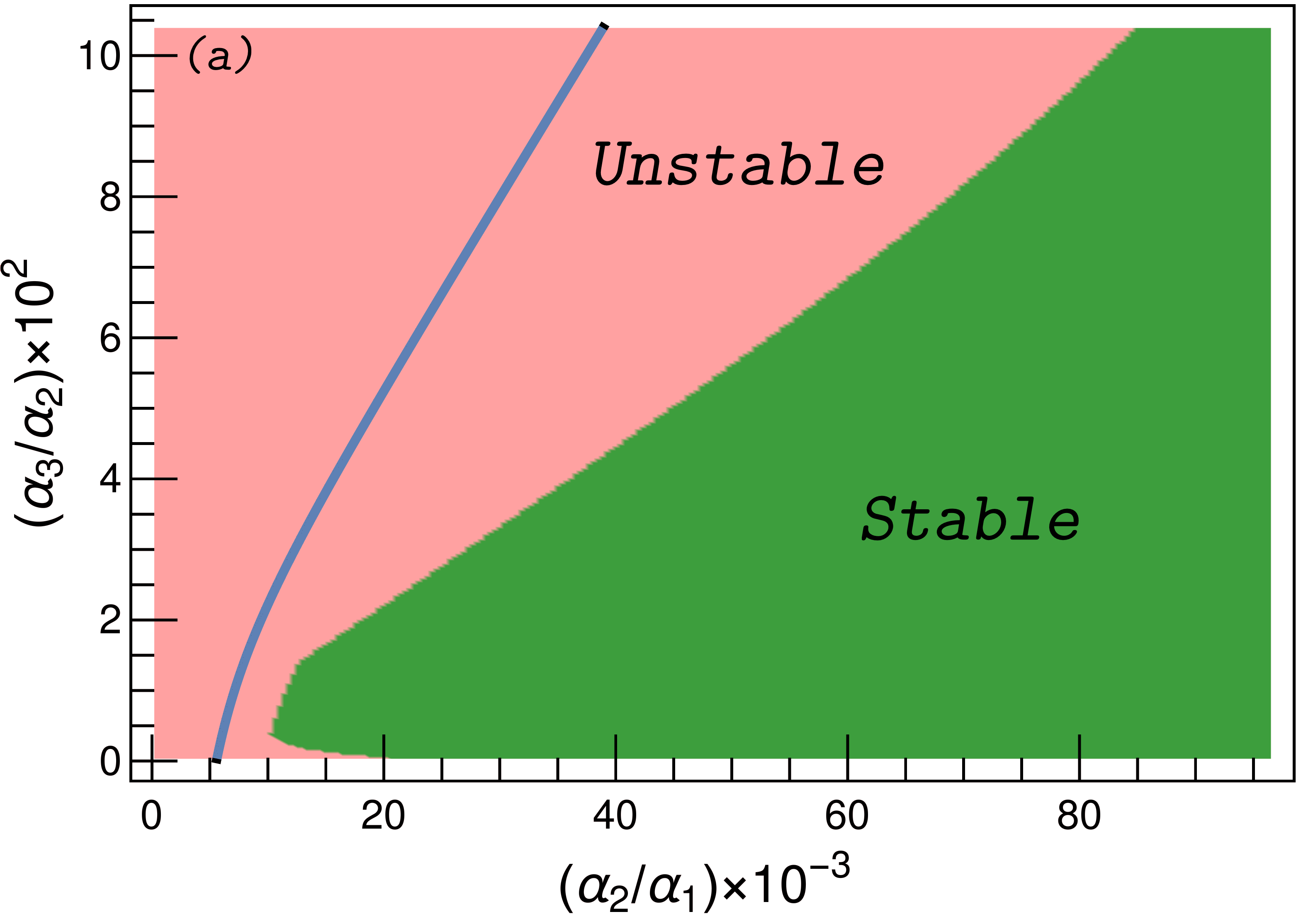
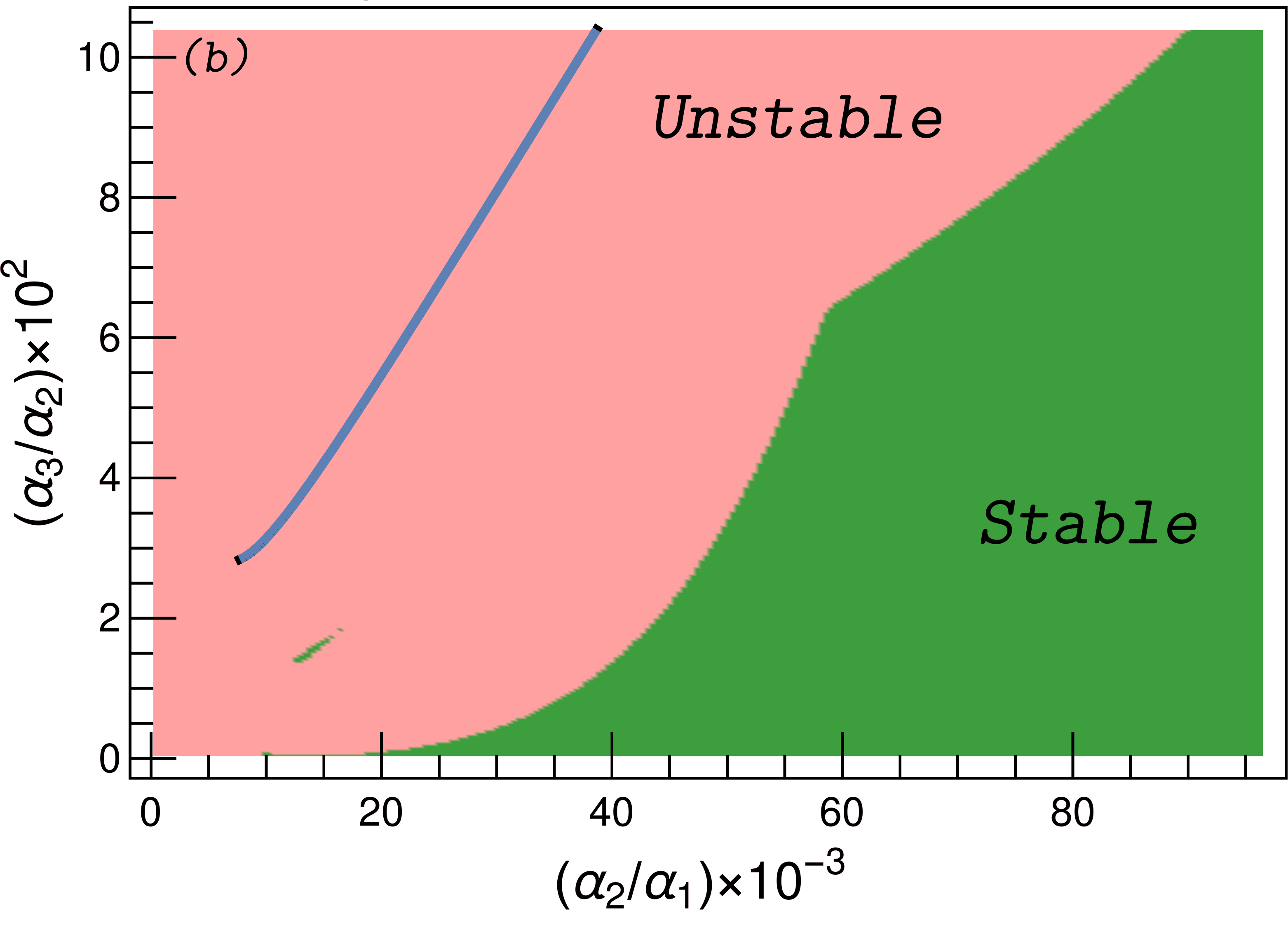
Figure 2: (color online). Stability phase diagram of the magnetic waveguide with self-generated offset field, for (a) $k=1$, $m=0$ and (b) $k=m=1$. The blue line is an estimation of the upper bound of the stability domain computed with Eq. (19). The threshold frequency corresponds to $\alpha_{2}/\alpha_{1}=\sqrt[3]{\Omega^{4}/2\omega_{\perp}^{4}}\approx 6\times 10^{3}$.

In addition, the steady periodic solution indicates that the magnetic moment of the atom is aligned along the $x$ axis since $\theta_{k}=k\pi$ and $\nu_{m}=(2m+1)\pi/2$. In fact this is not surprising, after all the self-generated offset field $\phi B_{\rm b}$ is oriented along this axis. The phase diagram shown in Fig. 2 represents the global stability of the investigated system. This implies that the actual extent of the stable domain, for a given situation, will be defined by how far the initial conditions are from the steady periodic solution around which we linearize the system dynamics. In other words, the atoms need to be injected in the stable orbits sustained by the guide.

The calculation of the stability boundary requires the knowledge of the analytical expressions of the eigenvalues of $\mathcal{M}$, which are very difficult to calculate for the actual problem. Therefore, the physical mechanisms participating in the stable guiding of the atoms are not easily accessible. Nevertheless, we can gain some intuition by applying the Lyapunov transformation $L(\tau)$

$$L(\tau)=\left(\begin{array}[]{cccccc}1&0&0&0&0&0\\ 0&1&0&0&0&0\\ 0&0&1&0&0&0\\ 0&0&0&1&0&0\\ 0&0&0&0&\cos[\beta(\tau)]&-\sin[\beta(\tau)]\\ 0&0&0&0&\sin[\beta(\tau)]&\cos[\beta(\tau)]\end{array}\right)\ ,$$ (17)

to the Eq. (13), with $\beta(\tau)$ defined by the equation

$$\dot{\beta}(\tau)+f(\alpha_{1},\alpha_{2},\alpha_{3},\tau)=1\ .$$ (18)

The Lyapunov transformation (17) does not reduce the linearized system given by Eq. (13) to a system with constant coefficients as it is usually desired kirillov . However, here is shown that it is enough for this transformation to be of Lyapunov-type to obtain the physical behavior of the system. Indeed, a Lyapunov transformation does not change the characteristic exponents of a linear system and preserve its regularity.

The function $\beta(\tau)$ is constrained to be periodic satisfying the condition $\beta(\pi)=\beta(2\pi)$, that translates into the following equation of state for the parameters of the system

$$\pi=(-1)^{k}\Big{[}\frac{(-1)^{k+m}}{2}\pi\alpha_{1}\alpha_{2}-2\alpha_{3}\Big{]}\ .$$ (19)

Then, using Eqs. (6), we can obtain the valid pairs of values ($\omega,\omega_{L})$ which set an upper bound for the stability domain for the case $k=1$, $m=0$ considered, for example, in Fig. 2(a). Indeed, in this particular case the Eq. (19) reads

$$\omega^{2}(\omega-\frac{2}{\pi}\omega_{L})-\frac{1}{2}\omega_{\perp}^{2}\Omega=0\ ,$$ (20)

from where we can conclude that since $\omega_{\perp}^{2}\Omega$ is always positive we must have $\omega>(2/\pi)\omega_{L}$. In Fig. 2(a) we have represented the curve (20) by the solid line which starts at $\omega_{th}=\sqrt[3]{\omega_{\perp}^{2}\Omega/2}$, approximately equal to $2\pi\times 3$ kHz for the parameter values considered in this particular example. Below this threshold frequency, the dynamics is unstable independently of the value of $\phi$. The same conclusion can be drawn from Fig. 2(b) calculated for $k=m=1$, where the same threshold frequency is observed. Therefore, the stable guiding in these situations requires a modulation frequency above the Larmor frequency. Finally, in Fig. 3 the stability phase diagram covering positive and negative values of $\alpha_{3}$ (or $\phi$) is presented for $k=0$, $m=0$. Comparing this figure with Fig. 2, we can notice the expected symmetry between $k$ even, $\alpha_{3}<0$ and $k$ odd, $\alpha_{3}>0$.

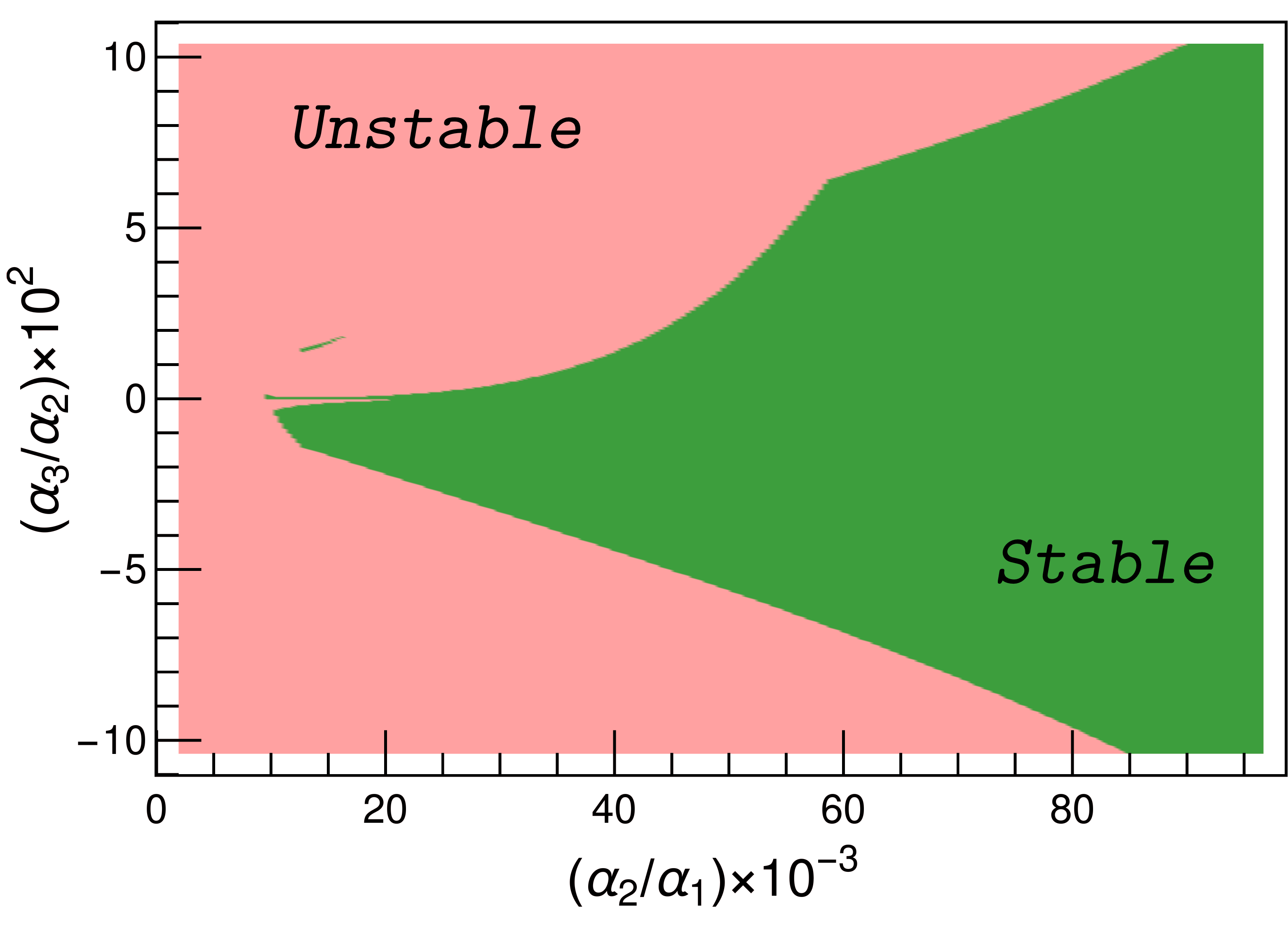
Figure 3: (color online). Stability phase diagram for $k=m=0$.

Here, we have demonstrated using formal arguments the existence of guiding stability domains in a magnetic waveguide created by a linear section of three concentric microwires carrying modulated currents. The striking point of this waveguide is that, in the absence of an external offset field, it can be made orbitally stable against atom losses by properly choosing the modulation frequency and the phase relationship between the currents. This unexpected emerging stability is established by analyzing the eigenvalues of the monodromy matrix of the dynamics linearized around a steady periodic solution. We found that the stability results from the interplay between the characteristic frequencies, as seen from the estimated limiting conditions obtained from a Lyapunov transformation of the system variables. More specifically, we found a lower bound for the modulation frequency determined by the Larmor frequency of the atoms. The next important question to be investigated is the coherence of matter waves during propagation in such a guide. We believe this work to be of relevance not only when considering the design of toroidal magnetic guides for high bandwidth rotation sensing with atom chips, but also for the design of complex miniature fast switching magnetic potentials for the study of low dimensional physics using atom chip based devices clga ; crookston ; fernholz .

This work was funded by the Délégation Générale de l’Armement (DGA) through the ANR ASTRID program (contrat ANR-13-ASTR-0031-01), the Institut Francilien de Recherche sur les Atomes Froids (IFRAF), the Emergence-UPMC program (contrat A1-MC-JC-2011/220).

- (1) R. C. Jaklevic, John Lambe, A. H. Silver, and J. E. Mercereau. Phys. Rev. Lett. 12, 159 (1964).
- (2) K. v. Klitzing, G. Dorda, and M. Pepper, Phys. Rev. Lett. 45, 494 (1980).
- (3) W. A. Prothero and J. M. Goodkind, Rev. Sci. Instrum. 39, 1257 (1968).
- (4) QuanS, http://www.muquans.com/
- (5) AOSense, http://aosense.com/
- (6) P. Gillot, O. Francis, A. Landragin, F. P. D. Santos, and S. Merlet, Metrologia 51, L15 (2014).
- (7) B. Canuel et al., Phys. Rev. Lett. 97, 010402 (2006).
- (8) M. Keil et al., J. Mod. Opt. 63, 1840 (2016), and references therein.
- (9) G. A. Sinuco-Leon and B. M. Garraway, New J. Phys. 18, 035009 (2016).
- (10) Y. Wang et al., Phys. Rev. A 96, 013630 (2017).
- (11) V. Y. F. Leung, A. Tauschinsky, N. J. van Druten, and R. J. C. Spreeuw, Quantum Inf. Process. 10, 955 (2011).
- (12) M. Ammar et al., Phys. Rev. A 91, 053623 (2015).
- (13) C.L. Garrido Alzar, W. Yan, and A. Landragin, Research in Optical Sciences, OSA Technical Digest, paper JT2A.10 (2012).
- (14) I. Lesanovsky et al., Phys. Rev. A 73, 033619 (2006).
- (15) T. Fernholz et al., Phys. Rev. A 75, 063406 (2007).
- (16) S. J. Kim et al., Phys. Rev. A 93, 033612 (2016).
- (17) G. J Dick, Local oscillator induced instabilities in the trapped ion frequency standards, Proc. 19th Precise Time and Time Interval (PTTI) Applications and Planning Meeting, Redondo Beach, CA, USA, 133 (1987).
- (18) J.-B. Trebbia et al., Phys. Rev. Lett. 98 , 263201 (2007).
- (19) I. Bouchoule et al., Phys. Rev. A 77, 023624 (2008).
- (20) J. Fortagh and C. Zimmermann, Rev. Mod. Phys. 79, 235 (2007).
- (21) S. Gov, S. Shtrikman, and H. Thomas, Am. J. Phys. 68, 334 (2000).
- (22) S. Gov and S. Shtrikman, J. Appl. Phys. 86, 2250 (1999).
- (23) R. Franzosi, B. Zambon and E. Arimondo, Phys. Rev. A 70, 053603 (2004).
- (24) F. Verhulst, Nonlinear Differential Equations and Dynamical Systems. Springer, Berlin (1990).
- (25) D. L. Lukes, Differential Equations: Classical to Controlled. Academic Press, New York (1982), Chapter 8.
- (26) H. Logemann and E. P. Ryan, Ordinary Differential Equations: Analysis, Qualitative Theory and Control. Springer, London (2014).
- (27) Oleg N. Kirillov, Nonconservative Stability Problems of Modern Physics (De Gruyter Studies in Mathematical Physics). Walter de Gruyter GmbH, Berlin/Boston (2013), Chapter 2.
- (28) M. B. Crookston et al., J. Phys. B: At. Mol. Opt. Phys. 38, 3289 (2005).