Nonnegative Low Rank Matrix Approximation for Nonnegative Matrices

Abstract

This paper describes a new algorithm for computing Nonnegative Low Rank Matrix (NLRM) approximation for nonnegative matrices. Our approach is completely different from classical nonnegative matrix factorization (NMF) which has been studied for more than twenty five years. For a given nonnegative matrix, the usual NMF approach is to determine two nonnegative low rank matrices such that the distance between their product and the given nonnegative matrix is as small as possible. However, the proposed NLRM approach is to determine a nonnegative low rank matrix such that the distance between such matrix and the given nonnegative matrix is as small as possible. There are two advantages. (i) The minimized distance by the proposed NLRM method can be smaller than that by the NMF method, and it implies that the proposed NLRM method can obtain a better low rank matrix approximation. (ii) Our low rank matrix admits a matrix singular value decomposition automatically which provides a significant index based on singular values that can be used to identify important singular basis vectors, while this information cannot be obtained in the classical NMF. The proposed NLRM approximation algorithm was derived using the alternating projection on the low rank matrix manifold and the non-negativity property. Experimental results are presented to demonstrate the above mentioned advantages of the proposed NLRM method compared the NMF method.

Keywords: Nonnegative matrix, low-rank approximation, manifolds, projections

AMS subject classiflcations. 15A23, 65f22.

1 Introduction

Nonnegative data matrices appear in many data analysis applications. For instance, in image analysis, image pixel values are nonnegative and the associated nonnegative image data matrices can be formed for clustering and recognition [5, 9, 10, 14, 15, 16, 19, 24, 25, 30, 34]. In text mining, the frequencies of terms in documents are nonnegative and the resulted nonnegative term-to-document data matrices can be constructed for clustering [3, 22, 27, 32]. In bioinformatics, nonnegative gene expression values are studied and nonnegative gene expression data matrices are generated for diseases and genes classification [6, 8, 11, 17, 18, 26, 31]. Nonnegative Low Rank Matrix (NLRM) approximation for nonnegative matrices play a key role in all these applications. Its main purpose is to identify a latent feature space for objects representation. The classification, clustering or recognition analysis can be done by using these latent features. Lee and Seung [19] proposed and developed Nonnegative Matrix Factorization (NMF) algorithms, and demonstrated that NMF has part-based representation which can be used for intuitive perception interpretation.

1.1 Related Work

NMF has emerged in 1994 by Paatero and Tapper [35] for performing environmental data analysis. The purpose of NMF is to decompose an input $m$-by-$n$ nonnegative matrix $A\in\mathbb{R}_{+}^{m\times n}$ into $m$-by-$r$ nonnegative matrix $B\in\mathbb{R}_{+}^{m\times r}$ and $r$-by-$n$ nonnegative matrix $C\in\mathbb{R}_{+}^{r\times n}$:

$$A\approx BC,$$

and

$$\min_{B,C\geq 0}\ \|A-BC\|^{2}_{F},$$ (1)

where $B,C\geq 0$ means that each entry of $B$ and $C$ is nonnegative, $\|\cdot\|_{F}$ is the Frobenius norm of a matrix, and $r$ (the low rank value) is smaller than $m$ and $n$. For simplicity, we assume that $m\geq n$, Several researchers have proposed and developed algorithms for determining such nonnegative matrix factorization in the literature. For instance, Lee and Seung [19, 20] proposed to solve NMF by using the multiplicative update algorithm by finding both $B$ and $C$ iteratively. Also Yuan and Oja [33] considered and studied a projective nonnegative matrix factorization and proposed the following minimization problem:

$$\min_{B\geq 0}\ \|A-BB^{T}A\|^{2}_{F},$$

where $B^{T}$ is the transpose of $B$. In the optimization problem, it is required to find a projection matrix $BB^{T}$ such that the difference between the given nonnegative matrix $A$ and its projection $BB^{T}A$ is as small as possible.

We remark that there can be many possible solutions in (1). In practice, it is necessary to impose additional constraints for finding NMF. In some applications, orthogonality, sparsity and/or smoothness constraints on $B$ and/or $C$ are incorporated in (1). Because of these constraint formulations, many optimization techniques have been designed to solve these minimization problems. For example, the multiplicative update algorithms [7, 8, 10] are revised to deal with these constraint minimization problems.

1.2 The Contribution

The proposed Nonnegative Low Rank Matrix (NLRM) approximation method is completely different from classical NMF. Here NLRM approximation is to find a nonnegative low rank matrix $X$ such that $X\approx A$ such that their difference is as small as possible. Mathematically, it can be formulated as the following optimization problem

$$\min_{\operatorname{rank}({X})=r,{X}\geq 0}\ \|{A}-{X}\|_{\textrm{F}}^{2}.$$ (2)

There are two advantages in the proposed NLRM method.

• It is obvious in (1) that when $B$ and $C$ are nonnegative, then the resulting matrix $BC$ is also nonnegative. But these constraints are more restricted than that required in (2). Instead of using NMF in (1), we study NLRM in (2). The distance $\|{A}-{X}\|_{\textrm{F}}^{2}$ by the proposed NLRM method can be smaller than $\min_{B,C\geq 0}\ \|A-BC\|^{2}_{F}$ by the NMF method. It implies that the proposed NLRM method can obtain a better low rank matrix approximation.

• The proposed NLRM approximation admits a matrix singular value decomposition, i.e.,

  $$X=U\Sigma V^{T},$$ (3)

  where $U$ is an $m$-by-$n$ matrix, $\Sigma$ is an $n$-by-$n$ diagonal matrix, and $V^{T}$ is also an $n$-by-$n$ matrix. The columns of $U$ are called the left singular vectors of the singular value decomposition $\{u_{i}\}_{i=1}^{m}$. These left singular vectors form an orthonormal basis system in $\mathbb{R}^{m\times m}$ such that $u_{i}^{T}u_{j}=1$ if $i=j$, otherwise 0. The rows of $V^{T}$ refer to the elements of the right singular vectors of the singular value decomposition $\{v_{i}\}_{i=1}^{n}$. These right singular vectors also form an orthonormal basis system in $\mathbb{R}^{n\times n}$ such that $v_{i}^{T}v_{j}=1$ if $i=j$, otherwise 0. The diagonal elements of $\Sigma=\ {\rm diag}(\sigma_{1},\sigma_{2},\cdots,\sigma_{n})$ are called the singular values. As $X$ is a rank $r$ matrix, we have $\sigma_{i}\geq 0$ for $1\leq i\leq r$ and $\sigma_{i}=0$ for $r+1\leq i\leq n$. The ordering of the singular values follows the descending order, i.e., $\sigma_{1}\geq\sigma_{2}\geq\cdots,\geq\sigma_{r}$. We remark that both $U$ and $V$ are not necessary to be nonnegative, but the resulting matrix $X=U\Sigma V^{T}$ must be non-negative. Therefore, this decomposition is different from principal component analysis as there is such requirement in principal component analysis. According to the singular value decomposition of $X$, the proposed method can identify important singular basis vectors based on singular values. In the classical NMF, this information cannot be obtained directly.

Our experimental results are presented to demonstrate the above mentioned advantages of the proposed NLRM method compared the NMF method.

The paper is organized as follows. In Section 2, we present our algorithm and show the convergence. In Section 3, numerical results are presented to demonstrate the proposed algorithm. Finally, some concluding remarks and future research work are given in Section 4.

2 The Optimization on Manifolds

Constrained optimization is quite well studied as an area of research, and many powerful methods are proposed to solve the general problems in that area. In some special cases, the constrain sets possess particularly rich geometric properties, i.e., they are manifolds in the meaning of classical differential geometry. Then some constrained optimization problems can be rewritten as optimizing a real-valued function $f(x)$ on a manifold ${\cal{M}}$:

$$\min_{x\in{\cal M}}f(x).$$ (4)

Here, ${\cal M}$ can be the Stiefel manifold, the Grassmann manifold and the fixed rank matrices manifold and so on. In order to better understand manifolds and some related definitions, e.g., charts, atlases and tangent spaces, we refer to [21] and the references therein. In general, the dimensions that some classical constrained techniques work are much bigger than the corresponding manifold (see e.g., [1, 28]).

2.1 The Algorithm

Alternating projection method is popular in searching a point in the intersection of convex sets because of its simplicity and intuitive appeal. Its basic idea is iteratively projecting a point one set and then the other. In contrast to the well known cases, this paper concerns with the extensions of convex sets to non-convex sets. Here, one set is the $m\times n$ fixed rank matrices manifold

$$\mathcal{M}_{r}:=\left\{X\in\mathbb{R}^{m\times n},\operatorname{rank}(X)=r\right\},$$ (5)

and the other one is the convex set of $m\times n$ nonnegative matrices

$$\mathcal{M}_{n}:=\left\{X\in\mathbb{R}^{m\times n},X_{i,j}\geq 0,i=1,...,m,j=1,...,n\right\}.$$ (6)

In order to introduce the main algorithm, we need to define two projections that project the given matrix onto $\mathcal{M}_{r}$ and $\mathcal{M}_{n}$, respectively. By the Eckart-Young-Mirsky theorem [12], the projection onto fixed rank matrix set $\mathcal{M}_{r}$ can be expressed as follows:

$$\pi_{1}({X})=\sum_{i=1}^{r}\sigma_{i}(X)u_{i}(X){v}_{i}^{T}(X),$$ (7)

where $\sigma_{i}(X)$ is the $i$-th singular values of $X$, and their corresponding left and right singular vectors: $u_{i}(X)$ and $v_{i}(X)$. The projection onto the nonnegative matrix set $\mathcal{M}_{n}$ can be expressed as follows:

$$\pi_{2}({X})=\left\{\begin{array}[]{c}X_{ij},~{}~{}~{}{\rm if}~{}~{}X_{ij}\geq 0,\\ 0,~{}~{}~{}~{}~{}{\rm if}~{}~{}X_{ij}<0.\end{array}\right.$$ (10)

In particular, since the manifold $\mathcal{M}_{r}$ is not convex, the projection mapping $\pi_{1}(X)$ can no longer be single valued (for example when the $r$-th singular value has multiplicity higher than 1). Then the algorithm of alternating projection on $\mathcal{M}_{r}$ and $\mathcal{M}_{n}$ can be given as Algorithm 1. The framework of this algorithm is the same as the general case, while the only difference is that the projections are respectively chosen as $\pi_{1}$ and $\pi_{2}$ given in (7) and (10).

Algorithm 1 Alternating Projections On Manifolds

Input: Given a nonnegative matrix ${A}\in\mathbb{R}^{m\times n}$ this algorithm computes nearest rank-$r$ nonnegative matrix.
  1: Initialize ${X}_{0}=A$;
  2: for $k=1,2,...$
  3:  ${Y}_{k+1}=\pi_{1}({X}_{k});$
  4:  ${X}_{k+1}=\pi_{2}({Y}_{k+1});$
  5: end
Output: ${X}_{k}$ when the stopping criterion is satisfied.

We note in Algorithm 1 that the projection of a given matrix onto the manifold $\mathcal{M}_{r}$ is done by truncating small singular values in the singular value decomposition of the given matrix. The computational complexity of this procedure is of $(mnr)$ operations.

Different from the convex sets case, the intersection of $\mathcal{M}_{r}$ and $\mathcal{M}_{n}$ decides whether the sequence generated by Algorithm 1, converges or not. In order to show the convergence of Algorithm 1, we compute the dimension of the intersection of $\mathcal{M}_{r}$ and $\mathcal{M}_{n}$.

Theorem 1.

Let $\mathcal{M}_{r}$ and $\mathcal{M}_{n}$ be defined as (5)-(6). Then

$$\mathcal{M}_{rn}:=\mathcal{M}_{r}\cap\mathcal{M}_{n}=\left\{X\in\mathbb{R}^{m\times n},~{}\operatorname{rank}(X)=r,~{}X_{ij}\geq 0,~{}i=1,...,m,j=1,...,n\right\}$$ (11)

is a smooth manifold with dimension $(m+n)r-r^{2}$.

The proof of Theorem 1 can be found in Supplementary. Moreover, we need to define the angle $\alpha(A)$ of $A\in\mathcal{M}_{rn}$ where

$$\alpha(A)=cos^{-1}(\sigma(A))\quad{\rm and}\quad\sigma(A)=\lim_{\xi\rightarrow 0}\sup_{B_{1}\in F^{\xi}_{1}(A),B_{2}\in F^{\xi}_{2}(A)}\left\{\frac{\left<B_{1}-A,B_{2}-A\right>}{\|B_{1}-A\|_{F}\|B_{2}-A\|_{F}}\right\},$$

with

$$F_{1}^{\xi}(A)=\{B_{1}\ |\ B_{1}\in\mathcal{M}_{r}\backslash A,\|B_{1}-A\|_{F}\leq\xi,B_{1}-A\bot T_{\mathcal{M}_{r}\cap\mathcal{M}_{n}}(A)\},$$

$$F_{2}^{\xi}(A)=\{B_{2}\ |\ B_{2}\in\mathcal{M}_{n}\backslash A,\|B_{2}-A\|_{F}\leq\xi,B_{2}-A\bot T_{\mathcal{M}_{r}\cap\mathcal{M}_{n}}(A)\},$$

and $T_{\mathcal{M}_{r}\cap\mathcal{M}_{n}}(A)$ is the tangent space of $\mathcal{M}_{r}\cap\mathcal{M}_{n}$ at point $A$ (the definition of the tangent space can be found in Supplemary). The angle is calculated based on the two points belonging $\mathcal{M}_{1}$ and $\mathcal{M}_{2}$ respectively.

A point $A$ in $\mathcal{M}_{rn}$ is nontangential if $\alpha(A)$ has a positive angle [2], i.e., $0\leq\sigma(A)<1$. It is interesting to note that if there is one nontangential point, majority of points are also nontangential because of the manifold smoothness. We show that $\mathcal{M}_{rn}$ contains a non-empty set $\mathcal{M}^{nt}_{rn}$ of nontangential points. The proof can be found in Supplementary.

Theorem 2.

$\mathcal{M}^{nt}_{rn}\neq\emptyset$.

By using this property, Andersson and Carlsson [2] have shown the following theorem.

Theorem 3.

Let $\mathcal{M}_{r}$, $\mathcal{M}_{n}$ and $\mathcal{M}_{rn}$ be given as (5), (6) and (11), the projections onto $\mathcal{M}_{r}$ and $\mathcal{M}_{rn}$ be given as (7)-(10), respectively. Denote $\pi$ as the projection onto $\mathcal{M}_{rn}$. Suppose that $P\in\mathcal{M}^{nt}_{rn}$ is a non-tangential intersection point, then for any given $\epsilon>0$ and $1>c>\sigma(P)$, there exist an $\xi>0$ such that for any ${A}\in Ball({P},\xi)$ (the ball neighborhood of $P$ with radius $\xi$ contains the given nonnegative matrix $A$) the sequence $\{{X}_{k}\}_{k=0}^{\infty}$ generated by the alternating projection algorithm initializing from given $A$ satisfies the following results:

1. the sequence converges to a point $X_{\infty}\in{\cal M}_{rn}$,

2. $\|{X}_{\infty}-\pi({A})\|_{F}\leq\epsilon\|{A}-\pi({A})\|_{F}$,

3. $\|{X}_{\infty}-{X}_{k}\|_{F}\leq{\rm const}\cdot c^{k}\|{A}-\pi({A})\|_{F}$,

where $\pi(A)\equiv{\rm argmin}_{\operatorname{rank}({X})=r,{X}\geq 0}\ \|{A}-{X}\|_{\textrm{F}}^{2}$ (the optimized solution).

According to Theorem 3, we know Algorithm 1 can converge and find a matrix that can be sufficiently close the best nonnegative approximation $\pi({A})$.

3 Numerical Results

In this section, we conducted several experiments to demonstrate that the proposed NLRM method can obtain a better low rank matrix approximation, and can provide a significant index based on singular values that can be used to identify important singular basis vectors in the approximation.

3.1 The First Experiment

In the first experiment, we randomly generated $m$-by-$r$ nonnegative matrices $B$ and $r$-by-$n$ nonnegative matrices $C$ where their matrix entries follow a uniform distribution in between 0 and 1. The given non-negative matrix $A$ was computed by the multiplication of $B$ with $C$. We employed the proposed NLRM algorithm (Algorithm 1) to test the relative residual $\|A-X_{c}\|_{F}/\|A\|_{F}$ and compared with testing NMF algorithms: A-MU [13], HALS [4], A-HALS [13], PG [23] and A-PG [23]. Here $X_{c}$ are the computed solutions by different algorithms.

Tables 1-3 shows the relative residuals of the computed solutions from the proposed algorithm and the testing NMF algorithms for synthetic data sets of sizes 100-by-80, 200-by-160 and 500-by-400 respectively. When there is no noise (the second column in the tables), the input data matrix $A$ is exactly a nonnegative rank $r$ matrix. Therefore, the proposed NLRM algorithm can provide exact recovery results in the first iteration. However, there is no guarantee that other testing NMF algorithms can determine the underlying nonnegative low rank factorization. In the tables, it is clear that the testing NMF algorithms cannot obtain the underlying low rank factorization. One of the reason may be that NMF algorithms can be sensitive to initial guesses. In the tables, we illustrate this phenomena by displaying the mean relative residual and the range containing both the minimum and the maximum relative residuals by using ten initial guesses randomly generated. We find in the tables that the relative residuals computed by the proposed NLRM algorithm are always smaller than the minimum relative residuals by the testing NMF algorithms.

On the other hand, the performance of the proposed algorithm was evaluated when a Gaussian noise of zero mean and variance $\sigma$ ($=0.001,0.005,0.01$) were added in the generated matrices $A$. The relative residuals of the computed solutions by the proposed NLRM algorithm and the other NMF algorithms are reported in Tables 1-3. We see from the tables that the relative residuals computed by the proposed method are always smaller than the minimum relative residuals by the testing NMF algorithms. All these results show that the performance of the proposed NLRM algorithm is better than that of the testing NMF algorithms.

Table 1: The relative residuals $\|A-X_{c}\|_{F}/\|A\|_{F}$ by different algorithms for 100-by-80 synthetic data matrices with several noise levels.

	$r=10$
Method	no noise	$\sigma=0.001$	$\sigma=0.005$	$\sigma=0.01$
NLRM	9.15e-16	1.72e-04	8.62e-04	1.70e-03
A-MU (mean)	1.43e-03	1.43e-03	1.68e-03	2.26e-03
A-MU (range)	[8.66e-04, 2.30e-03]	[8.85e-04, 2.30e-03]	[1.20e-03, 2.50e-03]	[1.90e-03, 2.90e-03]
HALS (mean)	1.36e-03	1.38e-03	1.63e-03	2.22e-03
HALS (range)	[7.22e-04, 2.30e-03]	[7.33e-04, 2.30e-03]	[1.10e-03, 2.40e-03]	[1.80e-03, 2.90e-03]
A-HALS (mean)	1.25e-03	1.37e-03	1.61e-03	2.23e-03
A-HALS (range)	[6.84e-04, 2.40e-03]	[5.22e-04, 2.30e-03]	[5.22e-04, 2.30e-03]	[6.84e-04, 2.40e-03]
PG (mean)	1.06e-03	8.24e-04	1.26e-03	1.96e-03
PG (range)	[2.36e-04, 2.00e-03]	[3.03e-04, 2.00E-03]	[9.39e-04, 1.80e-03]	[1.80e-03, 2.20e-03]
A-PG (mean)	2.03e-03	2.04e-03	2.21e-03	2.66e-03
A-PG (range)	[1.40e-03, 2.90e-03]	[1.40e-03, 2.90e-03]	[1.60e-03, 3.00e-03]	[2.20e-03, 3.40e-03]
	$r=20$
Method	no noise	$\sigma=0.001$	$\sigma=0.005$	$\sigma=0.01$
NLRM	8.32e-16	1.22e-04	6.07e-04	1.20e-03
A-MU (mean)	2.20e-04	2.54e-04	6.49e-04	1.21e-03
A-MU (range)	[9.74e-05, 4.41e-04]	[1.56e-04, 4.51e-04]	[6.15e-04, 7.36e-04]	[1.20e-03, 1.30e-03]
HALS (mean)	2.16e-04	2.53e-04	6.51e-04	1.22e-03
HALS (range)	[5.93e-05, 5.00e-04]	[1.36e-04, 4.98e-04]	[6.10e-04, 7.47e-04]	[1.20e-03, 1.30e-03]
A-HALS (mean)	5.47e-05	1.42e-04	6.12e-04	1.20e-03
A-HALS (range)	[2.29e-05, 1.19e-04]	[1.25e-04, 1.88e-04]	[6.09e-04, 6.20e-04]	[1.20e-03, 1.20e-03]
PG (mean)	1.15e-04	1.40e-04	6.17e-04	1.20e-03
PG (range)	[4.33e-05, 1.76e-04]	[1.22e-04, 1.90e-04]	[6.08e-04, 6.41e-04]	[1.20e-03, 1.20e-03]
A-PG (mean)	5.23e-04	5.37e-04	8.06e-04	1.32e-03
A-PG (range)	[3.30e-04, 6.98e-04]	[3.51e-04, 7.10e-04]	[6.90e-04, 9.30e-04]	[1.30e-03, 1.40e-03]
	$r=40$
Method	no noise	$\sigma=0.001$	$\sigma=0.005$	$\sigma=0.01$
NLRM	2.61e-15	8.43e-05	4.21e-04	8.43e-04
A-MU (mean)	1.82e-03	1.84e-03	1.92e-03	2.03e-03
A-MU (range)	[1.20e-03, 2.30e-03]	[1.20e-03, 2.30e-03]	[1.30e-03, 2.50e-03]	[1.60e-03, 2.40e-03]
HALS (mean)	2.82e-03	2.83e-03	2.87e-03	3.00e-03
HALS (range)	[2.40e-03, 3.20e-03]	[2.40e-03, 3.30e-03]	[2.50e-03, 3.30e-03]	[2.60e-03, 3.40e-03]
A-HALS (mean)	1.33e-05	8.64e-05	4.23e-04	8.43e-04
A-HALS (range)	[1.31e-06, 7.48e-05]	[8.43e-05, 9.35e-05]	[4.21e-04, 4.35e-04]	[8.43e-04, 8.44e-04]
PG (mean)	4.39e-04	2.42e-04	4.84e-04	1.02e-03
PG (range)	[4.07e-05, 7.64e-04]	[9.74e-05, 7.83e-04]	[4.23e-04, 6.98e-04]	[8.44e-04, 1.70e-03]
A-PG (mean)	3.40e-04	3.64e-04	5.87e-04	9.48e-04
A-PG (range)	[2.15e-06, 1.00e-03]	[8.43e-05, 1.00e-03]	[4.21e-04, 1.10e-03]	[8.43e-04, 1.30e-03]

Table 2: The relative residuals $\|A-X_{c}\|_{F}/\|A\|_{F}$ by different algorithms for 200-by-160 synthetic data matrices with several noise levels.

	$r=10$
Method	no noise	$\sigma=0.001$	$\sigma=0.005$	$\sigma=0.01$
NLRM	5.25e-16	1.33e-04	6.67e-04	1.30e-03
A-MU (mean)	3.38e-03	3.39e-03	3.45e-03	3.65e-03
A-MU (range)	[1.70e-03, 4.90e-03]	[1.80e-03, 4.90e-03]	[1.90e-03, 4.90e-03]	[2.30e-03, 5.00e-03]
HALS (mean)	4.49e-03	4.48e-03	4.47e-03	4.61e-03
HALS (range)	[3.30e-03, 6.00e-03]	[3.30e-03, 5.90e-03]	[3.40e-03, 5.60e-03]	[3.50e-03, 5.70e-03]
A-HALS (mean)	4.07e-03	4.23e-03	4.10e-03	4.05e-03
A-HALS (range)	[2.30e-03, 5.70e-03]	[3.00e-03, 5.30e-03]	[2.80e-03, 5.60e-03]	[2.50e-03, 5.70e-03]
PG (mean)	2.79e-03	2.09e-03	1.97e-03	2.60e-03
PG (range)	[8.70e-04, 4.10e-03]	[2.67e-04, 4.10e-03]	[1.00e-03, 3.40e-03]	[1.50e-03, 4.40e-03]
A-PG (mean)	3.02e-03	3.03e-03	3.24e-03	3.39e-03
A-PG (range)	[6.98e-04, 5.20e-03]	[7.09e-04, 5.20e-03]	[9.58e-04, 5.20e-03]	[1.50e-03, 5.40e-03]
	$r=20$
Method	no noise	$\sigma=0.001$	$\sigma=0.005$	$\sigma=0.01$
NLRM	6.41e-15	9.24e-05	4.62e-04	9.25e-04
A-MU (mean)	1.73e-03	1.73e-03	1.80e-03	1.97e-03
A-MU (range)	[1.40e-03, 2.50e-03]	[1.40e-03, 2.50e-03]	[1.50e-03, 2.60e-03]	[1.70e-03, 2.70e-03]
HALS (mean)	1.55e-03	1.55e-03	1.63e-03	1.82e-03
HALS (range)	[1.40e-03, 1.70e-03]	[1.40e-03, 1.70e-03]	[1.50e-03, 1.80e-03]	[1.70e-03, 2.00e-03]
A-HALS (mean)	1.29e-03	1.39e-03	1.40Ee-03	1.63e-03
A-HALS (range)	[1.00e-03, 1.70e-03]	[1.10e-03, 1.80e-03]	[8.55e-04, 1.80e-03]	[1.40e-03, 1.90e-03]
PG (mean)	1.80e-03	1.92e-03	1.73e-03	1.88e-03
PG (range)	[1.40e-03, 2.30e-03]	[1.60e-03, 2.10e-03]	[1.50e-03, 2.10e-03]	[1.60e-03, 2.30e-03]
A-PG (mean)	9.84e-04	9.86e-04	1.10e-03	1.35e-03
A-PG (range)	[7.59e-04, 1.20e-03]	[7.65e-04, 1.20e-03]	[9.02e-04, 1.30e-03]	[1.20e-03, 1.50e-03]
	$r=40$
Method	no noise	$\sigma=0.001$	$\sigma=0.005$	$\sigma=0.01$
NLRM	8.76e-16	6.28e-05	3.14e-04	6.28e-04
A-MU (mean)	6.05e-04	6.09e-04	6.84e-04	8.74e-04
A-MU (range)	[5.26e-04, 6.61e-04]	[5.31e-04, 6.64e-04]	[6.16e-04, 7.30e-04]	[8.24e-04, 9.08e-04]
HALS (mean)	3.54e-03	3.56e-03	3.63e-03	3.72e-03
HALS (range)	[2.90e-03, 4.80e-03]	[2.90e-03, 4.80e-03]	[2.90e-03, 4.90e-03]	[2.90e-03, 5.10e-03]
A-HALS (mean)	2.37e-05	6.88e-05	3.15e-04	6.28e-04
A-HALS (range)	[1.51e-05, 4.15e-05]	[6.37e-05, 8.13e-05]	[3.14e-04, 3.17e-04]	[6.28e-04, 6.29e-04]
PG (mean)	3.05e-03	2.84e-03	3.21e-03	3.22e-03
PG (range)	[1.70e-03,4.70e-03]	[1.30e-03, 6.10e-03]	[1.40e-03, 5.70e-03]	[1.50e-03, 5.20e-03]
A-PG (mean)	6.05e-04	6.09e-04	6.83e-04	8.74e-04
A-PG (range)	[5.04e-04, 7.43e-04]	[5.07e-04, 7.46e-04]	[5.93e-04, 8.06e-04]	[8.05e-04, 9.71e-04]

Table 3: The relative residuals $\|A-X_{c}\|_{F}/\|A\|_{F}$ by different algorithms for 500-by-400 synthetic data matrices with several noise levels.

	$r=10$
Method	no noise	$\sigma=0.001$	$\sigma=0.005$	$\sigma=0.01$
NLRM	1.33e-15	8.07e-05	4.03e-04	8.07e-04
A-MU (mean)	1.21e-03	1.22e-03	1.28e-03	1.47e-03
A-MU (range)	[6.06e-04, 3.00e-03]	[6.14e-04, 3.00e-03]	[7.38e-04, 3.10e-03]	[1.00e-03, 3.20e-03]
HALS (mean)	4.05e-03	4.09e-03	4.14e-03	4.34e-03
HALS (range)	[1.00e-03, 6.60e-03]	[1.10e-03, 6.60e-03]	[1.10e-03, 6.70e-03]	[1.30e-03, 8.40e-03]
A-HALS (mean)	3.39e-03	4.33e-03	3.45e-03	4.14e-03
A-HALS (range)	[1.10e-03, 5.80e-03]	[8.69e-04, 6.60e-03]	[8.58e-04, 5.00e-03]	[1.20e-03, 6.90e-03]
PG (mean)	5.17e-03	5.38e-03	4.52e-03	5.71e-03
PG (range)	[2.60e-03, 7.60e-03]	[2.40e-03, 7.40e-03]	[1.50e-03, 6.20e-03]	[2.40e-03, 7.30e-03]
A-PG (mean)	3.26e-04	3.74e-04	4.22e-04	8.15e-04
A-PG (range)	[3.93e-05, 2.30e-03]	[9.01e-05, 2.50e-03]	[4.06e-04, 4.54e-04]	[8.08e-04, 8.31e-04]
	$r=20$
Method	no noise	$\sigma=0.001$	$\sigma=0.005$	$\sigma=0.01$
NLRM	1.56e-15	5.81e-05	2.91e-04	5.81e-04
A-MU (mean)	4.38e-03	4.38e-03	4.38e-03	4.42e-03
A-MU (range)	[4.10e-03, 4.80e-03]	[4.10e-03, 4.80e-03]	[4.10e-03, 4.80e-03]	[4.20e-03, 4.80e-03]
HALS (mean)	4.67e-03	4.67e-03	4.69e-03	4.73e-03
HALS (range)	[4.40e-03, 5.00e-03]	[4.40e-03, 5.00e-03]	[4.40e-03, 5.00e-03]	[4.40e-03, 5.10e-03]
A-HALS (mean)	4.32e-03	4.29e-03	4.48e-03	4.41e-03
A-HALS (range)	[3.80e-03, 4.70e-03]	[4.10e-03, 4.50e-03]	[4.20e-03, 4.90e-03]	[4.10e-03, 4.80e-03]
PG (mean)	8.87e-03	9.03e-03	8.82e-03	8.82e-03
PG (range)	[8.10e-03, 9.60e-03]	[8.30e-03, 1.01e-02]	[8.10e-03, 9.60e-03]	[8.10e-03, 9.40e-03]
A-PG (mean)	4.58e-03	4.58e-03	4.59e-03	4.61e-03
A-PG (range)	[4.10e-03, 5.10e-03]	[4.10e-03, 5.10e-03]	[4.10e-03, 5.10e-03]	[4.20e-03, 5.10e-03]
	$r=40$
Method	no noise	$\sigma=0.001$	$\sigma=0.005$	$\sigma=0.01$
NLRM	1.78e-15	4.10e-05	2.05e-04	4.10e-04
A-MU (mean)	2.10e-03	2.10e-03	2.10e-03	2.11e-03
A-MU (range)	[1.90e-03, 2.30e-03]	[1.90e-03, 2.30e-03]	[1.90e-03, 2.30e-03]	[1.90e-03, 2.30e-03]
HALS (mean)	5.58e-03	5.58e-03	5.51e-03	5.46e-03
HALS (range)	[4.50e-03, 7.10e-03]	[4.50e-03, 7.10e-03]	[4.50e-03, 7.20e-03]	[4.20e-03, 7.20e-03]
A-HALS (mean)	2.05e-03	1.98e-03	2.26e-03	1.78e-03
A-HALS (range)	[1.60e-03, 3.30e-03]	[1.40e-03, 2.70e-03]	[1.50e-03, 5.00e-03]	[1.50e-03, 2.60e-03]
PG (mean)	7.53e-03	7.83e-03	7.74e-03	7.77e-03
PG (range)	[6.60e-03, 8.90e-03]	[6.80e-03, 8.90e-03]	[6.70e-03, 9.00e-03]	[6.60e-03, 9.70e-03]
A-PG (mean)	2.55e-03	2.55e-03	2.56e-03	2.60e-03
A-PG (range)	[2.50e-03, 2.70e-03]	[2.50e-03, 2.70e-03]	[2.50e-03, 2.70e-03]	[2.50e-03, 2.70e-03]

3.2 The Second Experiment

In the second experiment, we randomly generated $m$-by-$n$ nonnegative matrices $A$ where their matrix entries follow a uniform distribution in between 0 and 1. The low rank minimizer is unknown in this setting. Table 4 shows that the relative residuals $\|A-X_{c}\|_{F}/\|A\|_{F}$ of the computed solution $X_{c}$ from the proposed NLRM algorithm and the testing NMF algorithms. In the testing NMF algorithms, we use 10 different initial guesses and report the results of the mean and the range (the minimum and the maximum values) of the relative residuals in the tables. We see from Table 4 that the relative residuals computed by the proposed NLRM method are smaller than the minimum relative residuals by the testing NMF algorithms. All these results show that the performance of the proposed NLRM algorithm is better than that of the testing NMF algorithms.

Moreover, we considered the CBCL face database [36]. In the face database, there are $m=2469$ facial images, each consisting of $n=19\times 19=361$ pixels, and constituting a face image matrix $A\in\mathbb{R}_{+}^{361\times 2469}$. We tested several values of $r=20,40,60,80$ for nonnegative low rank minimization and compared the proposed NLRM algorithm with the testing NMF algorithms. In the testing NMF algorithms, we used 10 different initial guesses and report the results of relative residuals of the mean and the range in the tables. We see from Table 5 that the relative residuals computed by the proposed NLRM method are smaller than the minimum relative residuals by the testing NMF algorithms. Again the performance of the proposed algorithm is better than that of the testing NMF algorithms.

Table 4: The relative residuals $\|A-X_{c}\|_{F}/\|A\|_{F}$ by different algorithms for synthetic data matrices.

	$m=100$, $n=80$
Method	$r=10$	$r=20$	$r=40$
NLRM	0.4047	0.3228	0.1874
A-MU (mean)	0.4087	0.3434	0.2487
A-MU (range)	[0.4086, 0.4089]	[0.3428, 0.3447]	[0.2477, 0.2502]
HALS (mean)	0.4087	0.3426	0.2448
HALS (range)	[0.4086, 0.4088]	[0.3421, 0.3431]	[0.2438, 0.2458]
A-HALS (mean)	0.4087	0.3424	0.2449
A-HALS (range)	[0.4086, 0.409]	[0.342, 0.3427]	[0.2437, 0.2462]
PG (mean)	0.4087	0.3422	0.2445
PG (range)	[0.4086, 0.4089]	[0.3418, 0.3426]	[0.2425, 0.2465]
A-PG (mean)	0.4088	0.3428	0.2450
A-PG (range)	[0.4086, 0.4091]	[0.3420, 0.3436]	[0.2442, 0.2463]
	$m=200$, $n=160$
Method	$r=10$	$r=20$	$r=40$
NLRM	0.4503	0.4054	0.3252
A-MU (mean)	0.4522	0.4151	0.3586
A-MU (range)	[0.4521, 0.4523]	[0.4148, 0.4156]	[0.358, 0.3591]
HALS (mean)	0.4522	0.4149	0.3569
HALS (range)	[0.4521, 0.4523]	[0.4147, 0.4151]	[0.3565, 0.3574]
A-HALS (mean)	0.4522	0.4149	0.3568
A-HALS (range)	[0.4521, 0.4523]	[0.4145, 0.4152]	[0.3565, 0.3572]
PG (mean)	0.4521	0.4147	0.3568
PG (range)	[0.4521, 0.4522]	[0.4145, 0.415]	[0.3564, 0.3572]
A-PG (mean)	0.45215	0.41478	0.35741
A-PG (range)	[0.4521, 0.4522]	[0.4146, 0.4151]	[0.3569, 0.3582]
	$m=500$, $n=400$
Method	$r=10$	$r=20$	$r=40$
NLRM	0.4803	0.4607	0.4238
A-MU (mean)	0.4807	0.4635	0.4357
A-MU (range)	[0.4807, 0.4807]	[0.4634, 0.4635 ]	[0.4357, 0.4358]
HALS (mean)	0.4807	0.4633	0.4352
HALS (range)	[0.4807, 0.4808]	[0.4633, 0.4634]	[0.4352, 0.4353]
A-HALS (mean)	0.4807	0.4634	0.4352
A-HALS (range)	[0.4807, 0.4807]	[0.4633, 0.4634]	[0.4351, 0.4353]
PG (mean)	0.4807	0.4633	0.4353
PG (range)	[0.4807, 0.4807]	[0.4633, 0.4634]	[0.4351, 0.4354]
A-PG (mean)	0.4807	0.4634	0.4353
A-PG (range)	[0.4807 0.4807]	[0.4633, 0.4635]	[0.4352, 0.4354]

Table 5: The relative residuals $\|A-X_{c}\|_{F}/\|A\|_{F}$ by different algorithms for face data.

	$m=361$, $n=2469$
Method	$r=20$	$r=40$	$r=60$	$r=80$
NLRM	0.1170	0.0839	0.0654	0.0529
A-MU (mean)	0.1220	0.0911	0.0751	0.0639
A-MU (range)	[0.1218, 0.1222]	[0.0907, 0.0914]	[0.0746, 0.0755]	[0.0632, 0.0651]
HALS (mean)	0.1220	0.0902	0.0721	0.0598
HALS (range)	[0.1218, 0.1224]	[0.09, 0.0905]	[0.0719, 0.0723]	[0.0596, 0.0601]
A-HALS (mean)	0.1220	0.0901	0.0719	0.0595
A-HALS (range)	[0.1217, 0.1222]	[0.0898, 0.0904]	[0.0717, 0.072]	[0.0594, 0.0597]
PG (mean)	0.1219	0.0902	0.0740	0.0633
PG (range)	[0.1217, 0.122]	[0.0899, 0.0909]	[0.0731, 0.0747]	[0.0626, 0.0645]
A-PG (mean)	0.1221	0.0908	0.0754	0.0658
A-PG (range)	[0.1218, 0.1226]	[0.0905, 0.0913]	[0.075, 0.0757]	[0.0652, 0.0684]

3.3 The Third Experiment

In practice, it is necessary to determine the value of rank for nonnegative matrix approximation. In this experiment, we show the advantage of the proposed NLRM algorithm for providing a significant index based on singular values that can be used to identify important singular basis vectors in the approximation.

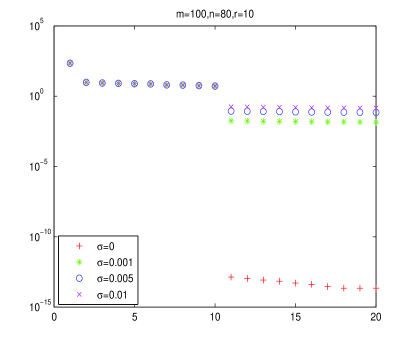
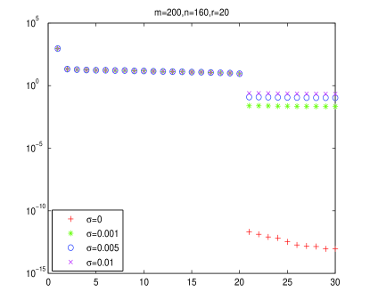
    (a)                    (b)

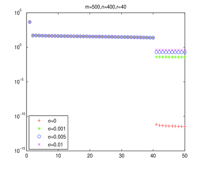
(c)

Figure 1: The distribution of singular values of (a) the generated 100-by-80 matrix with actual rank 10, (b) the generated 200-by-160 matrix actual rank 20, and (c) the generated 500-by-400 matrix with actual rank 40.

Similar to the first experiment, we randomly generated $m$-by-$n$ nonnegative matrices with actual ranks ($10,20,40$) and added Gaussian noise of zero mean and variance $\sigma$. In Figure 1, we display the distribution of singular values of the matrix approximation with rank $r$ ($=20,30,50$) for the generated 100-by-80 matrix with actual rank 10, 200-by-160 matrix with actual rank 20, and 500-by-400 matrix with actual rank 40 respectively. In this setting, we employ a matrix approximation with rank $r$ ($=20,30,50$) being larger than the actual rank ($=10,20,40$) of the generated nonnegative matrix. When there is no noise ($\sigma=0$), we see from Figures 1(a), 1(b), and 1(c) that there is a big jump in between the $k$-th singular value and the $(k+1)$th singular value for actual ranks $k=10$, $k=20$, and $k=40$ respectively. When there is a noise ($\sigma=0.001,0.005,0.01$), there is still a jump in between the $k$-th singular value and the $(k+1)$th singular value ($k$ is the actual rank), and the height of the jump depends on the noise level. This observation is also valid for other randomly generated matrices in the first experiment. According to these figures, the distribution of singular values can provide us information to determine a suitable low rank matrix approximation.

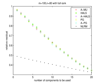
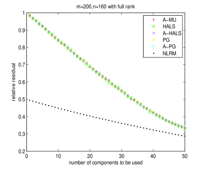
    (a)                    (b)

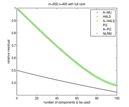
(c)

Figure 2: The comparison of relative residuals with respect to the number of components to be used in the matrix approximation with (a) $r=20$ for the generated 100-by-80 matrix, (b) $r=50$ for the generated 200-by-160 matrix, and (c) $r=100$ for the generated 500-by-400 matrix.

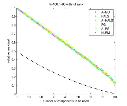
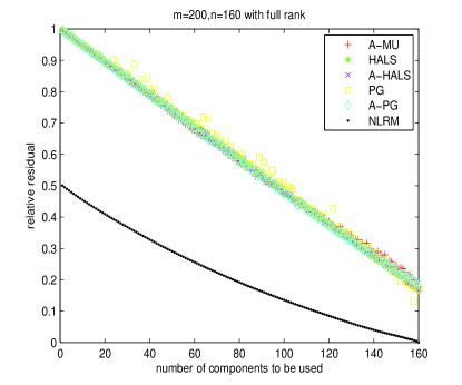
    (a)                    (b)

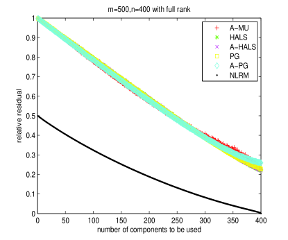
(c)

Figure 3: The comparison of relative residuals with respect to the number of components to be used in the matrix approximation with (a) $r=80$ for the generated 100-by-80 matrix, (b) $r=160$ for the generated 200-by-160 matrix, and (c) $r=400$ for the generated 500-by-400 matrix.

On the other hand, we randomly generated $m$-by-$n$ nonnegative matrices with full rank. In Figures 2-3, we display the relative residuals of the use of different numbers of the computed singular vectors by the proposed NLRM algorithm. More precisely, the computed solution is given as follows: $X_{c}=\sum_{i=1}^{r}\sigma_{i}u_{i}v_{i}^{T}$. We plot $\|A-X_{c}(j)\|_{F}/\|A\|_{F}$ with respect to $j$ (the number of singular vectors to be used in the matrix approximation), where $X_{c}(j)=\sum_{i=1}^{j}\sigma_{i}u_{i}v_{i}^{T}$ in the figures. Note that we employ singular vectors $u_{i}$ and $v_{i}^{T}$ according to the descending order of the singular values $\sigma_{i}$ ($\sigma_{1}\geq\sigma_{2}\geq\cdots\geq\sigma_{j}$). We see from the figures that when $j$ increases, the corresponding relative residual decreases. These results show that the matrix approximation to the given nonnegative matrix according to the ordering of singular values, is an effective strategy. As a reference, when $r$ is equal to the full rank number, the relative residual by the proposed NLRM algorithm, is close to the machine precision (around 1e-16). In contrast, there is no index to show the columns of $m$-by-$r$ computed matrix $B_{comp}$ and the rows of $r$-by-$n$ computed matrix $C_{comp}$ in the NMF approximation $B_{comp}C_{comp}$ to the nonnegative matrix $A$. Here we normalize the row vectors of $C_{comp}$ such that the sum of squares of each row of $C_{comp}$ is equal to 1, and then reorder the resulting column vectors of $B_{comp}$ according to their sum of squares. We plot $\|A-X_{nmf}(j)\|_{F}/\|A\|_{F}$ with respect to $j$ where $X_{nmf}(j)=\sum_{i=1}^{j}[B_{comp}](:,i)[C_{comp}](i,:)$ and $[B_{comp}](:,i)$ is the $i$-th column of reordered $B_{comp}$ and $[C_{comp}](i,:)$ is the $i$-th row of the normalized $C_{comp}$. In Figures 2-3. In the figures, we see that when $j$ increases, the relative residual decreases by the testing NMF algorithms. However, their relative residuals are still larger than those by the proposed NLRM algorithm. It is interesting to note that even $r$ is equal to the full rank number of the given nonnegative matrix, the relative residuals computed by the testing NMF algorithms are not close to the machine precision. The reason may be that there is no guarantee that the testing NMF algorithms give global optimal solutions.

Also we computed the relative residuals for face data matrix by the above mentioned procedure in Figure 4. We see from the figure that the relative residuals by the proposed NLRM algorithm are significantly smaller than those by the testing NMF algorithms for different values of $r=20,40,60,80,361$. According to Figures 2-4, we summarize that the proposed NLRM algorithm can provide a significant index based on singular values that can be used to identify important singular basis vectors in the approximation.

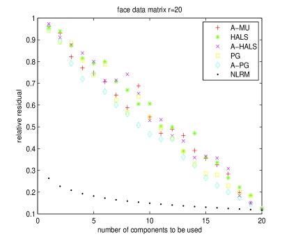
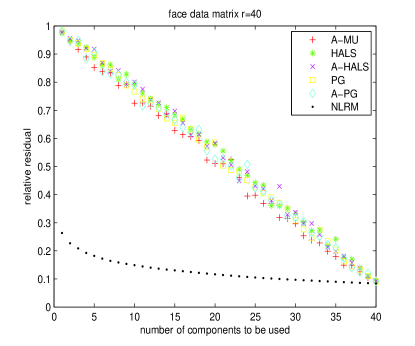
    (a)                    (b)

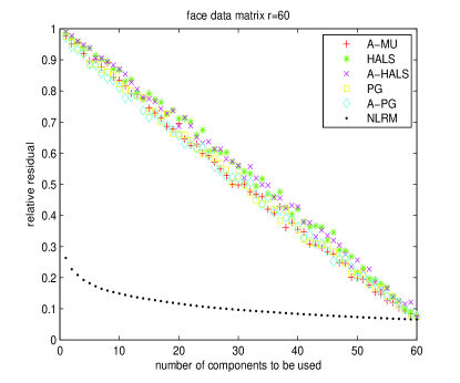
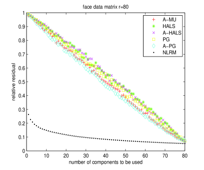
    (c)                    (d)

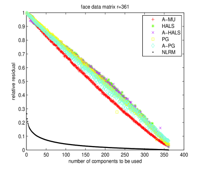
(e)

Figure 4: The comparison of relative residuals with respect to the number of components to be used in the face data matrix approximation with (a) $r=20$ (b) $r=40$ (c) $r=60$ (d) $r=80$ (e) $r=361$ (full rank).

4 Concluding Remarks

In this paper, we proposed and developed a new algorithm for computing NLRM approximation for nonnegative matrices. The new method is different from classical nonnegative matrix factorization method. We have shown the convergence of the proposed algorithm based on the results in manifold. Moreover, we have demonstrated numerical results that the minimized distance by the proposed NLRM method can be smaller than that by the NMF method. According to the ordering of singular values, the proposed method identifies important singular basis vectors, while this information cannot be obtained in the classical NMF. As a future research work, there are several areas to be studied:

1. The computational cost of the proposed method involves the computation of singular value decomposition. We plan to study tangent space method for low rank matrix projection so that the computational complexity can be reduced for large scale data science applications.

2. We study applications of nonnegative low rank matrix approximation and check how the proposed method can provide a significant index based on singular values that can be used to identify important singular basis vectors in the approximation.

3. In classical NMF applications, researchers have suggested to use the other norms (such as $l_{1}$ norm and KL divergence) in data fitting $\|A-BC\|$ instead of Frobenius norm to deal with other machine learning applications. It is interesting to develop the related algorithms for nonnegative low rank matrix approximation.

Supplementary Information

The supplementary information consists of the theoretical proofs of Theorems 1-3.

Some basic definitions, propositions of algebraic geometry and differential geometry are needed to prove the main results. We only provide some results here and for details we refer to [1, 21] and references therein.

In order to show the convergence of Algorithm 1, we need to prove the intersection of $\mathcal{M}_{r}$ given as (5) and $\mathcal{M}_{n}$ given as (6) is a manifold first. In many real applications, some manifolds are actually real algebraic varieties which are defined as the vanishing of a set of polynomials on $\mathbb{R}^{n}$, thus some algebraic geometry methods can help us to study the above problem. Note that all complex varieties are real varieties, but not conversely. For a given real algebraic variety $\mathcal{V}\in\mathbb{R}^{n}$, if we identity $\mathbb{R}^{n}$ as a subset of $\mathbb{C}^{n}$ and denote $\mathbb{I}_{\mathbb{R}}(\mathcal{V})$ as the set of real polynomials that vanish on $\mathcal{V}$, then $\mathcal{V}$ has a related complex variety given by its Zariski closure

$$\mathcal{V}_{Zar}=\{z\in\mathbb{C}^{n}:p(z)=0,\ \forall p\in\mathbb{I}_{\mathbb{R}}(\mathcal{V})\},$$

which is defined as the subset in $\mathbb{C}^{n}$ of common zeros to all polynomials that vanish on $\mathcal{V}$. Moreover, H. Whitney in [29] showed that a real algebraic variety $\mathcal{V}$ can be decomposed as $\mathcal{V}=\bigcup_{j=0}^{m}\mathcal{V^{\prime}}_{j}$ where each $\mathcal{V^{\prime}}_{j}$ is either void or a $\mathbb{C}^{(\infty)}$-manifold with dimension $j$. If $\mathcal{V^{\prime}}_{m}\neq\emptyset$, then $m$ equals the algebraic dimension of $\mathcal{V}_{Zar}$. Each $\mathcal{V^{\prime}}_{j}$ contains at most a finite number of connected components. This result shows that the main part of a variety is a manifold.

Varieties have singular points which is different from manifolds. Note that a point $A\in\mathcal{V}$ is nonsingular if it is nonsingular in the sense of algebraic geometry as an element of $\mathcal{V}_{zar}$. This result changes to be much simpler, if we restrict on the irreducible variety. Here a algebraic variety $\mathcal{V}$ is said to be irreducible if there does not exist non-trivial real algebraic varieties $\mathcal{V}^{\prime}_{1}$ and $\mathcal{V}^{\prime}_{2}$, such that $\mathcal{V}=\mathcal{V}^{\prime}_{1}\bigcup\mathcal{V}^{\prime}_{2}$. Denote $\nabla$ as the gradient operator and set ${\cal N}_{\cal V}(z)=\{\nabla p(z):p\in\mathbb{I}_{\mathbb{R}}(\mathcal{V})\}$. Suppose that $\mathcal{V}\in\mathbb{R}^{n}$ is an irreducible real algebraic variety of dimension $m$, then $\dim{\cal N}_{\mathcal{V}}(z)\leq n-m$ and $z\in\mathcal{V}$ is non-singular if and only if $\dim{\cal N}_{\mathcal{V}}(z)=n-m$. In practice, it is not easy to check a given variety is irreducible or not, thus the following results are needed.

Definition 1 (Definition 6.7 in [2]).

Suppose we are given a number $j\in\mathbb{N}$ and an index set $I$ such that for each $i\in I$, there exist an open connected $\Omega_{i}\subseteq\mathbb{R}^{j}$ and a real analytic map $\phi_{i}:\Omega_{i}\rightarrow\mathcal{V}.$ Then $\mathcal{V}$ is said to be covered with analytic patches, if for each $A\in\mathcal{V},$ there exists an $i\in I$ and a radius $r_{A}$ such that

$$\mathcal{V}_{rn}\cap Ball_{\mathbb{R}^{n}}(A,r_{A})=Im\phi_{i}\cap Ball_{\mathbb{R}^{n}}(A,r_{A}).$$

Proposition 1 (Proposition 6.8 in [2]).

Let V be a real algebraic variety. If $\mathcal{V}$ is connected and can be covered with analytic patches, then $\mathcal{V}$ is irreducible.

Moreover, the following proposition proposed us a simple method to compute the dimensions of some varieties involved which are tricky to compute.

Proposition 2 (Proposition 6.9 in [2]).

Under the assumption of Proposition 1, suppose in addition that an open subset of $\mathcal{V}$ is the image of a bijective real analytic map defined on a subset of $\mathbb{R}^{d}$. Then $\mathcal{V}$ has dimension $d$.

With the above tools in hand we can prove the following results. The idea of the proof follows from [2].

Proof of Theorem 1: The proof can be divided into two parts. Firstly, we need to prove the following set

$$\mathcal{V}_{rn}=\left\{X\in\mathbb{R}^{m\times n},~{}\operatorname{rank}(X)\leq r,~{}X_{i,j}\geq 0,~{}i=1,...,m,j=1,...,n\right\}$$ (12)

is an irreducible variety with dimension $(m+n)r-r^{2}$. Then we need to prove $\mathcal{V}_{rn}^{ns}$ (the set of all the non-singular points in $\mathcal{V}_{rn}$) equals the set of all the nonnegative matrices with rank equal to $r$.

Denote $\mathcal{K}$ as set of $m\times n$ matrices over $\mathbb{R}$. If all elements of a matrix $A\in\mathcal{K}$ are considered as variables, $\mathcal{K}$ is a linear manifold with dimension $mn$. The same statement is also satisfied for the nonnegative matrix set $\mathcal{M}_{n}$. Denote $\mathcal{V}_{r}:=\left\{X\in\mathbb{R}^{m\times n},\ \operatorname{rank}(X)\leq r\right\}$. Recall that a matrix in $\mathcal{K}$ has rank being greater than $r$ if and only if one can find a nonzero $(r+1)\times(r+1)$ invertible minor. The determinant of each such minor is a polynomial, and $\mathcal{V}_{r}$ is clear the variety obtained from the collection of such polynomials. Thus $\mathcal{V}_{r}$ is a real algebraic variety. The same statement is also true for $\mathcal{V}_{rn}$, which is derived by adding that a matrix entry is the square of a variable (i.e., nonnegative constraints) to the variety defining on $\mathcal{V}_{r}$. In order to use Proposition 1, we need to show that $\mathcal{V}_{rn}$ is covered with analytic patches and connected, and then $\mathcal{V}_{rn}$ can be irreducible.

(i) (Covered with analytic patches) Denote $U\in\mathbb{R}^{m\times r^{\prime}}$, $V\in\mathbb{R}^{n\times r^{\prime}}$ and a diagonal matrix $\Sigma\in\mathbb{R}^{r^{\prime}\times r^{\prime}}$ where $r^{\prime}\leq r$. Here we assume $r^{\prime}\geq 1$. For $r^{\prime}=0$, it is a trivial case. Suppose that $\pi(i)=r^{\prime}$ for all $i=1,...,m$. We set $u_{i,\pi(i)}$ as an undetermined variable. Now we can construct a real analytic mapping $\theta$ from $\hat{U}$ (the first $(r^{\prime}-1)$ rows of $U$), $\Sigma$ and $V$ to $\mathcal{V}_{rn}$ as follows:

$$\theta(u_{1,1},u_{1,2},...,u_{1,r^{\prime}-1},...,u_{m,1},...,u_{m,r^{\prime}-1},\sigma_{1},...,\sigma_{r^{\prime}},v_{1,1},...,v_{n,r^{\prime}})$$ (25)

$$= \left(\begin{array}[]{cccc}u_{1,1}&\cdots&u_{1,r^{\prime}-1}&u_{1,r^{\prime}}\\ u_{2,1}&\cdots&u_{2,r^{\prime}-1}&u_{2,r^{\prime}}\\ \vdots&\ddots&\vdots&\vdots\\ u_{m,1}&\cdots&u_{m,r^{\prime}-1}&u_{m,r^{\prime}}\\ \end{array}\right)\left(\begin{array}[]{cccc}\sigma_{1}&0&\cdots&0\\ 0&\sigma_{2}&\cdots&0\\ \vdots&\vdots&\ddots&\vdots\\ 0&0&\cdots&\sigma_{r^{\prime}}\\ \end{array}\right)\left(\begin{array}[]{cccc}v_{1,1}&\cdots&v_{1,r^{\prime}-1}&v_{1,r^{\prime}}\\ v_{2,1}&\cdots&v_{2,r^{\prime}-1}&v_{2,r^{\prime}}\\ \vdots&\ddots&\vdots&\vdots\\ v_{n,1}&\cdots&v_{n,r^{\prime}-1}&v_{n,r^{\prime}}\\ \end{array}\right)^{T}.$$

Note that the entries of the matrix in (25) can be nonnegative when the associated inequalities of $m$ undetermined variables are satisfied. Such $m$ undetermined variables are decoupled in these inequalities. There are infinitely many real solutions of $m$ undetermined variables for given values of $\hat{U}$, $\Sigma$, and $V$. It is saying that $\mathcal{V}_{rn}$ is the image of $\theta$. Let $\Gamma$ be a particular connected component of $(\hat{U},\Sigma,V)$. We establish a function $\psi$ with $\pi$ and $\Gamma$ as follows:

$$\psi_{\pi,\Gamma}(y)=U(y)\Sigma(y)V(y)^{T},~{}~{}y\in\Gamma.$$ (27)

Denote $\mathbb{I}$ as the set of all possible $\pi$ and $\Gamma$. It can be found that for each matrix in $\mathcal{V}_{rn}$ is in the image of at least one $\psi_{\pi,\Gamma}$ where $(\pi,\Gamma)\in\mathbb{I}$. Then by Definition 1, $\mathcal{V}_{rn}$ can be covered by $\{\psi_{\pi,\Gamma}\}_{(\pi,\Gamma)\in\mathbb{I}}$.

(ii) (Connected) In order to show $\mathcal{V}_{rn}$ is connected, we need to show that for any two nonnegative matrices $A,B\in\mathcal{V}_{rn}$, there exist a continuous map $f$ from the unit interval $[0,1]$ to $\mathcal{V}_{rn}$ such that $f(0)=A$ and $f(1)=B$. Without loss of generality, we show that for an arbitrary $A\in\mathcal{V}_{rn}$, it is connected with 1 matrix (all the entries are equal to 1) instead. It is sufficient to prove $\mathcal{V}_{rn}$ is path connected. Suppose that $A,B\in\mathcal{V}_{rn}$ are arbitrary and path connected with the 1 matrix, respectively. Thus there are two continuous maps $f$ and $g$ which are from the unit interval $[0,1]$ to $\mathcal{V}_{rn}$ with $f(0)=A$, $f(1)=\textbf{1}$, $g(0)=\textbf{1}$ and $g(1)=B$. Setting $\tau(x)=(1-x)f(x)+xg(x)$, it is easy to see that $\tau(x)$ is continuous and satisfying $\tau(0)=f(0)=A$ and $\tau(1)=g(1)=B$. Then $\mathcal{V}_{rn}$ is path connected. Let $A\in\mathcal{V}_{rn}$. Suppose that all the singular values of $A$ are ordered decreasingly with $\sigma_{1}=1$ (if $\sigma_{1}\neq 1$, we can divide or multiply some factor such that $\sigma_{1}=1$. Set $\pi(i)=r^{\prime}=rank(A)$, $i=1,...,m$ as above and choose $\Gamma$ such that the matrix representation can be expressed as (27). Now if $\sigma_{2}\neq 1$, we can proceed until it is not without leaving $\Gamma$. Then the values of $y$ corresponding to the first and second column of $\hat{U}$ and $V$ can be continuously moved until all elements of the first column of $\hat{U}$ and $V$ are positive, respectively. At this point, we can reduce all values of $\hat{U}$ and $V$ except the first column to zero, increase the first value of each row whenever necessary to stay in $\Gamma$. Then we can move $y$ so that the values in the first column become the same. Finally, we can let these values increase simultaneously until they reach $1$. Then the matrix $\mathbf{1}$ is derived, which is saying that $\mathcal{V}_{rn}$ is connected. Hence it is irreducible.

(iii) Now we would like to apply Proposition 2 so that $\mathcal{V}_{rn}$ possesses dimension $(m+n)r-r^{2}$. Here we need to find an open subset of $\mathcal{V}_{rn}$ which can be expressed as the image of a bijective real analytic map defined on a subset of $\mathbb{R}^{(m+n)r-r^{2}}$. Now we set $\Upsilon$ as a subset of $\mathcal{V}_{rn}$ in which the matrix rank is $r$. There are $r$ singular values. According to (25) and the singular value decomposition theory [12], we know that for a matrix in $\Upsilon$, the columns of $\hat{U}$ are orthogonal and the dimension is $(mr-\frac{r(r+1)}{2}-m)$, and the rows of $V$ are orthogonal and the dimension is $(nr-\frac{r(r+1)}{2})$. In addition, there are $m$ undetermined variables in the last column of $U$, and there are $r$ independent variables on the main diagonal matrix $\Sigma$. Therefore, the combined dimension is $(m+n)r-r^{2}$. Now we can identify three sets of matrices with $\mathbb{R}^{mr-\frac{r(r+1)}{2}}$, $\mathbb{R}^{nr-\frac{r(r+1)}{2}}$ and $\mathbb{R}^{r}$ respectively. Denote the inverses of these identifications by

$$\iota_{1}:\mathbb{R}^{mr-\frac{r(r+1)}{2}}\rightarrow\mathbb{R}^{m\times r};~{}\iota_{2}:\mathbb{R}^{r}\rightarrow\mathbb{R}^{r\times r};~{}\iota_{3}:\mathbb{R}^{mr-\frac{r(r+1)}{2}}\rightarrow\mathbb{R}^{n\times r};$$ (28)

and denote $\Omega\subset\mathbb{R}^{(m+n)r-r^{2}}$ as the open set corresponding to those matrices having the same structure as $\Upsilon$. Define $\phi:\Omega\rightarrow\mathcal{V}_{rn}$ by

$$\phi(y_{1},y_{2},y_{3})=\iota_{1}(y_{1})\times\iota_{2}(y_{2})\times\iota_{3}(y_{3})^{T}.$$ (29)

It is easy to see that $\phi$ is bijective correspondence with an open set of $\mathcal{V}_{rn}$ and $\phi$ is a polynomial. By Proposition 2, $\mathcal{V}_{rn}$ possesses dimension $(m+n)r-r^{2}$ as desired.

In the second step, we mainly prove $\mathcal{V}_{rn}^{ns}$ equals all the nonnegative matrices with rank equal to $r$. Recall that $\mathcal{V}_{rn}$ is an irreducible real algebraic variety with dimension $(m+n)r-r^{2}$, then we need to prove

$$\dim\mathcal{N}_{\mathcal{V}_{rn}}(A)=mn-(m+n)r+r^{2},$$

if and only if $\operatorname{rank}(A)=r$. It is sufficient to show that $\dim\mathcal{N}_{\mathcal{V}_{rn}}(A)\leq mn-(m+n)r+r^{2}$ is strict when $\operatorname{rank}(A)<r$ and the reverse inequality holds when $rank(A)=r$. Now for a given polynomial $p\in\mathbb{I}(\mathcal{V}_{rn})$, and two orthogonal matrices $U$ and $V$, $q_{U,V}(\diamond)=p(U\diamond V^{T})$, which is also in $\mathbb{I}(\mathcal{V}_{rn})$. Let $A$ be a fixed nonnegative matrix with $\text{rank}(A)=k\leq r$. By using the singular value decomposition, we can produce two orthogonal matrices $U$ and $V$ such that

$$UAV^{T}=\operatorname{diag}\{\sigma_{1},...,\sigma_{k},0,...,0\}=E_{k},$$

where the first $k$ diagonal values of $E_{k}$ are positive numbers and $0$ otherwise. In particular $\nabla q_{U,V}(A)=U\nabla p(UAV^{T})V^{T}=U\nabla p(E_{k})V^{T}$, implying that $\dim\mathcal{N}_{\mathcal{V}_{rn}}(A)=\dim\mathcal{N}_{\mathcal{V}_{rn}}(E_{k})$. If $k=r,$ all the $(r+1)\times(r+1)$ subdeterminants of the matrices in $\mathcal{K}$ form polynomials in $\mathbb{I}(\mathcal{V}_{rn})$, thus

$$\dim\mathcal{N}_{\mathcal{V}_{rn}}(E_{r})\geq mn-(m+n)r+r^{2},$$

which proves that any rank $r$ element of $\mathcal{V}_{rn}$ is nonsingular. Moreover, if $k<r$, consider some fixed $u\in\mathbb{R}_{+}^{m}$ and $v\in\mathbb{R}_{+}^{n}$, define the map $\vartheta_{u,v}:\mathbb{R_{+}}\rightarrow\mathcal{V}_{rn}$ via $\vartheta_{u,v}(x)=E_{k}+xuv^{T}$. Considering

$$\dim\left\{Span\left\{\frac{d}{dx}\vartheta_{u,v}(0):u\in\mathbb{R}_{+}^{m},v\in\mathbb{R}_{+}^{n}\right\}\right\}=mn,$$

hence $\dim\mathcal{N}_{\mathcal{V}_{rn}}(E_{k})=0$, which shows that $E_{k}$ is singular.

Combine the above conclusions, we can get $\mathcal{V}_{rn}$ is an irreducible real algebraic variety with dimension $(m+n)r-r^{2}$, and $\mathcal{V}_{rn}^{ns}$ is a $\mathbb{C}^{\infty}$-manifold of dimension $(m+n)r-r^{2}$. $\quad\Box$

Proof of Theorem 2: Suppose that the angle $\alpha(A)$ of $A\in\mathcal{M}_{r}\cap\mathcal{M}_{n}$ is well defined, then $A$ is tangential if $\alpha(A)=0$, and is nontangetial if $\alpha(A)>0$. Moreover, $A\in\mathcal{M}_{r}\cap\mathcal{M}_{n}$ is nontangential if and only if

$$\mathcal{T}_{\mathcal{M}_{r}}(A)\cap\mathcal{T}_{\mathcal{M}_{n}}(A)=\mathcal{T}_{\mathcal{M}_{r}\cap\mathcal{M}_{n}}(A),$$ (30)

where $\mathcal{T}_{\mathcal{M}_{r}}(A)$ and $\mathcal{T}_{\mathcal{M}_{n}}(A)$ denote the differential geometry tangent spaces of manifolds $\mathcal{M}_{r}$ and $\mathcal{M}_{n}$ at point $A,$ respectively. Denote $\mathcal{M}_{rn}^{nt}\subseteq\mathcal{M}_{rn}$ as the set of all nontangential points of $\mathcal{M}_{r}\cap\mathcal{M}_{n}$. Recall that the tangent space of $\mathcal{M}_{r}$ at $A=U_{m\times r}\cdot\Sigma_{r\times r}\cdot V_{n\times r}^{T}$ can be expressed as

$${\cal T}_{{\cal M}_{r}}(A)=\left\{[U,U_{\bot}]\left(\begin{array}[]{cc}\mathbb{R}^{r\times r}&\mathbb{R}^{r\times(n-r)}\\ \mathbb{R}^{(m-r)\times r}&0^{(m-r)\times(n-r)}\\ \end{array}\right)[V,V_{\bot}]^{T}\right\},$$

where $U_{\bot}\in\mathbb{R}^{m\times(m-r)}$ and $V_{\bot}\in\mathbb{R}^{n\times(n-r)}$ stand for the orthogonal completions of $U$ and $V,$ respectively. In addition, it is not difficult to derive $\mathcal{T}_{\mathcal{M}_{n}}(A)=Span\{E_{ij}\}$ with $E_{ij}=1$ or $0$, for all $i=1,...,m$ and $j=1,...,n$. Thus

$$\dim(\mathcal{T}_{\mathcal{M}_{r}}(A)\cap\mathcal{T}_{\mathcal{M}_{n}}(A))\leq(m+n)r-r^{2}.$$ (31)

Recall Theorem 1, $\mathcal{M}_{rn}$ is a smooth manifold with dimension $(m+n)r-r^{2}$, which is homeomorphism to its tangent space $\mathcal{T}_{\mathcal{M}_{rn}}(A)$. Thus,

$$\dim(\mathcal{T}_{\mathcal{M}_{r}}(A)\cap\mathcal{T}_{\mathcal{M}_{n}}(A))\leq\dim(\mathcal{T}_{\mathcal{M}_{rn}}(A)),$$ (32)

which is sufficient to say $\mathcal{M}_{rn}^{nt}$ is not empty.$\quad\Box$

Note that $\mathcal{V}_{rn}$ is an irreducible variety with dimension $(m+n)r-r^{2}$, and $\mathcal{M}_{rn}^{nt}$ is not empty, then it follows from Theorem 6.6 in [2] that $\mathcal{V}_{rn}\setminus\mathcal{M}_{rn}^{nt}$ is a real algebraic variety of dimension strictly less than $(m+n)r-r^{2}$. This result tell us the majority of points are nontangential if one is. Moreover, (32) is satisfied, then by Theorem 5.1 in [2], we can get Theorem 3.

References

- [1] Absil, P. A., Mahony, R. & Sepulchre, R. Optimization algorithms on matrix manifolds (Princeton University Press, 2009).
- [2] Andersson, F. & Carlsson, M. Alternating projections on nontangential manifolds. Constructive approximation, 38, 489-525 (2013).
- [3] Berry, M. W. & Kogan, J. Text Mining: Applications and Theory (West Sussex, PO19 8SQ, UK: John Wiley and Sons, 2010).
- [4] Cichocki, A., Zdunek, R. & Amari, S. Hierarchical ALS algorithms for nonnegative matrix and 3D tensor factorization. International Conference on Independent Component Analysis and Signal Separation, 169-176 (2007).
- [5] Chen, M., Chen, W. S., Chen, B. & Pan, B. Non-negative sparse representation based on block NMF for face recognition. In Chinese Conference on Biometric Recognition. Springer, Cham, 26-33 (2013).
- [6] Cho, H., Dhillon, I. S., Guan, Y. & Sra, S. Minimum sum squared residue based co-clustering of gene expression data. In Proc. 4th SIAM International Conference on Data Mining (SDM) Florida, 114-125 (2004).
- [7] Choi, S. Algorithms for orthogonal nonnegative matrix factorization. In 2008 IEEE International Joint Conference on Neural Networks (IEEE World Congress on Computational Intelligence) IEEE, 1828-1832 (2008).
- [8] Cichocki, A., Zdunek, R., Phan, A. H. & Amari, S. I. Nonnegative matrix and tensor factorizations: applications to exploratory multi-way data analysis and blind source separation (John Wiley and Sons, 2009).
- [9] Ding, C., He, X. & Simon, H. D. On the equivalence of nonnegative matrix factorization and spectral clustering. In Proc. SIAM International Conference on Data Mining (SDM’05), 606-610 (2005).
- [10] Ding, C., Li, T., Peng, W. & Park, H. Orthogonal nonnegative matrix tri-factorizations for clustering. In KDD06: Proceedings of the 12th ACM SIGKDD international conference on Knowledge Discovery and Data Mining. New York, NY, USA, ACM Press, 126-135 (2006).
- [11] Gao, Y. & Church, G. Improving molecular cancer class discovery through sparse non-negative matrix factorization. Bioinformatics 21(21), 3970-3975 (2005).
- [12] Golub, G. H. & Van Loan, C. F. Matrix computations (vol. 3, JHU Press, 2012).
- [13] Gillis, N. & Glineur, F. Accelerated multiplicative updates and hierarchical ALS algorithms for nonnegative matrix factorization. Neural computation 24(4), 1085-1108 (2012).
- [14] Guillamet, D. & Vitria, J. Non-negative matrix factorization for face recognition. In Topics in artificial intelligence. Springer Berlin Heidelberg, 336-344 (2002).
- [15] Guillamet, D., Vitria, J. & Schiele, B. Introducing a weighted nonnegative matrix factorization for image classification. Pattern Recognition Letters 24(14), 2447-2454 (2003).
- [16] Jing, L. P., Zhang, C. & Ng, M. K. SNMFCA: supervised NMF-based image classification and annotation. IEEE Transactions on Image Processing 21(11), 4508-4521 (2012).
- [17] Kim, P. M. & Tidor, B. Subsystem identification through dimensionality reduction of large-scale gene expression data. Genome Research 13, 1706-1718 (2003).
- [18] Kim, H. & Park, H. Sparse non-negative matrix factorizations via alternating non-negativity-constrained least squares for microarray data analysis. Bioinformatics 23(12), 1495-1502, 2007.
- [19] Lee, D. D. & Seung, H. S. Learning of the parts of objects by non-negative matrix factorization. Nature 401, 788-791 (1999).
- [20] Lee, D. D. & Seung, H. S. Algorithms for Nonnegative Matrix Factorization. MIT Press 13, (2001).
- [21] Lee, J. M. Smooth manifolds, in Introduction to Smooth Manifolds (Springer, 2013).
- [22] Li, T. & Ding, C. The relationships among various nonnegative matrix factorization methods for clustering. In Proc. 6th International Conference on Data Mining (ICDM06). Washington, DC, USA, IEEE Computer Society, 362-371 (2006).
- [23] Lin, C. J. Projected gradient methods for nonnegative matrix factorization. Neural computation 19(10), 2756-2779 (2007).
- [24] Liu, H., Wu, Z., Cai, D. & Huang, T. S. Constrained nonnegative matrix factorization for image representation. IEEE Transactions on Pattern Analysis and Machine Intelligence 34(7), 1299-1311 (2012).
- [25] Liu, Y., Jing, L. P. & Ng, M. K. Robust and non-negative collective matrix factorization for text-to-image transfer learning. IEEE Transactions on Image Processing 24(12), 4701-4714 (2015).
- [26] Pascual-Montano, A., Carmona-Saez, P., Chagoyen, M., Tirado, F., Carazo, J. M. & Pacual-Marqui, R. bioNMF: A versatile tool for non-negative matrix factorization in biology. BMC Bioinformatics 7(1) (2006).
- [27] Pauca, V. P., Shahnaz, F., Berry, M. W. & Plemmons, R. J. Text mining using non-negative matrix factorizations. In Proc. SIAM Inter. Conf. on Data Mining 4, 452-456 (2004).
- [28] Vandereycken, B. Low-rank matrix completion by riemannian optimization. SIAM Journal on Optimization 23, 1214-1236 (2013).
- [29] Whitney, H. Elementary structure of real algebraic varieties. The Annals of Mathematics 66, 545-556 (1957).
- [30] Wang, Y., Jia, Y., Hu, C. & Turk, M. Non-negative matrix factorization framework for face recognition. International Journal of Pattern Recognition and Artificial Intelligence 19(4), 495-511 (2005).
- [31] Wang, G., Kossenkov, A. V. & Ochs, M.F. LS-NMF: A modified non-negative matrix factorization algorithm utilizing uncertainty estimates. BMC Bioinformatics 7(175), (2006).
- [32] Xu, W., Liu. X. & Gong, Y. Document clustering based on non-negative matrix factorization, In SIGIR 03:Proceedings of the 26th annual international ACM SIGIR conference on Research and development in informaion retrieval. New York, NY, USA, ACM Press, 267-273 (2003).
- [33] Yuan, Z. & Oja, E. Projective nonnegative matrix factorization for image compression and feature extraction. In Scandinavian Conference on Image Analysis, Springer Berlin Heidelberg, 333-342 (2005).
- [34] Zhang, D., Chen, S. & Zhou, Z. H. Two-dimensional non-negative matrix factorization for face representation and recognition. Lecture Notes in Computer Science 3723, 350-363 (2005).
- [35] Paatero, P. & Tapper, U. Positive matrix factorization: A non-negative factor model with optimal utilization of error estimates of data values. Environmetrics 5, 111-126 (1994).
- [36] CBCL Face Database, MIT Center For Biological and Computation Leearning, http://www.ai.mit.edu/projects/cbcl.