Effects of diagonal strains and H-bond geometry in antiferroelectric squaric acid crystals

Abstract

The proton ordering model of the phase transition and physical properties of antiferroelectric crystals of squaric acid is modified by taking into account the influence of diagonal lattice strains and of the local geometry of hydrogen bonds, namely of the distance $\delta$ between the H-sites on a bond. Thermal expansion, the spontaneous strain $\varepsilon_{1}-\varepsilon_{3}$, and specific heat of squaric acid are well described by the proposed model. However, a consistent description of hydrostatic pressure influence on the transition temperature is possible only with further modifications of the model.

Key words: antiferroelectricity, hydrogen bond, phase transition, thermal expansion, hydrostatic pressure

Abstract

Çàïðîïîíîâàíî ìîäèôiêàöiþ ìîäåëi ïðîòîííîãî âïîðÿäêóâàííÿ, ÿêà ìàє íà ñâî¿ ìåòi îïèñ ôàçîâîãî ïåðåõîäó òà ôiçèчíèõ âëàñòèâîñòåé àíòèñåãíåòîåëåêòðèчíèõ êðèñòàëiâ êâàäðàòíî¿ êèñëîòè, ùî âðàõîâóє âïëèâ äiàãîíàëüíèõ êîìïîíåíò òåíçîðà äåôîðìàöié òà ëîêàëüíî¿ ãåîìåòði¿ âîäíåâèõ çâ’ÿçêiâ, à ñàìå âiääàëi $\delta$ ìiæ ïîëîæåííÿìè ðiâíîâàãè ïðîòîíà íà çâ’ÿçêó. Òåïëîâå ðîçøèðåííÿ, ñïîíòàííà äåôîðìàöiÿ $\varepsilon_{1}-\varepsilon_{3}$ òà òåïëîєìíiñòü êðèñòàëó äîáðå îïèñóþòüñÿ çàïðîïîíîâàíîþ ìîäåëëþ. Îäíàê îäíîчàñíèé îïèñ âïëèâó ãiäðîñòàòèчíîãî òèñêó íà òåìïåðàòóðó ôàçîâîãî ïåðåõîäó ìîæëèâèé ëèøå ïðè ïîäàëüøîìó óñêëàäíåííi ìîäåëi.

Ключовi слова: àíòèñåãíåòîåëåêòðèê, âîäíåâèé çâ’ÿçîê, ôàçîâèé ïåðåõiä, òåïëîâå ðîçøèðåííÿ, ãiäðîñòàòèчíèé òèñê

1 Introduction

The crystals of squaric acid, H₂C₄O₄ (3,4-dihydroxy-3-cyclobutene-1,2-dione) are an epitome of two-dimensional antiferroelectrics. The hydrogen bonded C₄O₄ groups form planes parallel to $ac$ and stacked along the $b$-axis. Below the transition at 373 K, a spontaneous polarization arises in these planes, with the neighbouring planes polarized in the opposite directions. The crystal symmetry changes from centrosymmetric tetragonal, $I4/m$, to monoclinic, $P2_{1}/m$, and spontaneous symmetry-changing strains $\varepsilon_{1}-\varepsilon_{3}$ (orthorhombic) and $\varepsilon_{5}$ (monoclinic), both of $B_{g}$ symmetry, arise [2, 1, 3]. The local symmetry of the H₂C₄O₄ groups is C_1h below and above the antiferroelectric phase transition [4].

Elastic and thermoelastic properties of squaric acid are remarkably anisotropic. Compressibility and thermal expansion [5] are much higher in a direction perpendicular to the planes of hydrogen bonds than within the planes. The symmetry-changing strains $\varepsilon_{1}-\varepsilon_{3}$ and $\varepsilon_{5}$ are confined to the $ac$ plane. The anomalous parts of the diagonal strains $\varepsilon_{1}$, $\varepsilon_{3}$ and of $\varepsilon_{2}$, caused by electrostriction, have different signs.

There is also experimental evidence for non-equivalence of hydrogen bonds going along two perpendicular directions (e.g. [6, 1]). The difference between degrees of proton ordering on these bonds is about 2% at $T_{\textrm{N}}-13$ K and $T_{\textrm{N}}-21$ K [1]. The O–H and H-site distances are also found to be slightly different for the perpendicular bonds.

Hydrostatic pressure rapidly decreases the antiferroelectric transition temperature with the slope of about 11 K/kbar [7, 8, 4] at pressures below about 25 kbar. At higher pressures, this dependence deviates from linearity, and around 28 kbar, the transition temperature rapidly falls to zero: a quantum paraelectric state is induced [4]. At further increase of pressure at a constant temperature (at least for temperatures between 100 and 300 K), another phase boundary is detected [4], at which the local symmetry of the H₂C₄O₄ groups changes from C_1h to C_4h.

Theoretical description of the antiferroelectric transition in squaric acid is usually based on some versions of the proton ordering model, either two-dimensional, invoking four-particle correlations between protons within the planes [9, 10, 11, 12], or one-dimensional, where either non-interacting [13] or coupled [14] perpendicular pseudospin chains are considered. The four-particle model can be reduced to the model of interacting one-dimensional chains by the proper choice of the model parameters [13]. The four-particle Hamiltonians are basically identical to those for NH₄H₂PO₄ crystals, antiferroelectrics of the KH₂PO₄ family.

Deformational effects in squaric acid were first addressed in [9, 10, 11], where the coupling between spins and spontaneous lattice distortion were included into the model. In [12] the proton-phonon coupling was added, and hydrostatic pressure effects on the phase transition temperature and dielectric permittivity of pure and deuterated squaric acid crystals were described by assuming the model parameters to be pressure dependent and by performing a new fitting procedure for each considered value of pressure.

In [15, 16], the observed in [4] $p-T$ phase diagram comprising the antiferroelectric phase with the C₄O₄ groups having the local symmetry C_1h, the paraelectric phase (C_1h), and high-pressure paraelectric phase (C_4h), was qualitatively described, using different versions of proton ordering model. The intermediate paraelectric phase (C_1h) was found to be a quantum liquid-like state.

Since the antiferroelectric phase transition in squaric acid is usually attributed to proton ordering, which triggers displacements of heavy ions and rearrangement of electronic density, it is expected that just like in the KH₂PO₄ family crystals, in the squaric acid the pressure-induced changes in the geometry of the hydrogen bonds should play an important role in the pressure influence on the phase transition. The distance $\delta$ between the two equilibrium positions of a proton on a hydrogen bond was found to be the most crucial geometrical parameter here [17, 18]. For the KH₂PO₄ family crystals, having a three-dimensional network of hydrogen bonds, there exists a universal linear dependence of the transition temperatures $T_{c}$ on the value of the distance $\delta$ at the transition, with $T_{c}$ and $\delta$ being varied by external hydrostatic pressure, uniaxial stress $p=-\sigma_{3}$, and by isomorphic substitution of heavy ions [17, 18]. For the squaric acid, which H-bond network is two-dimensional, the dependence $T_{c}(\delta)$ under hydrostatic pressure is similar but with a different slope.

None of the above mentioned earlier theories for the squaric acid crystals explicitly considers the role of the geometrical parameters of hydrogen bonds in the pressure effects on the phase transition in squaric acid. None of them includes into consideration the thermal expansion of the crystal either.

Thus, similarly to how it was done for Rochelle salt [19], we intend to develop a unified deformable model for squaric acid that can describe the effects associated with the diagonal lattice strains: thermal expansion and influence of external hydrostatic pressure. We shall also include the dependence of the interaction constants on the H-site distance $\delta$ into the model.

An important question arises whether tunneling of protons on hydrogen bonds, also known to be essentially dependent on their geometry, should be taken into account in the model. We believe that for the reasons described below, at temperatures and pressures considered in the present paper it will suffice to use an Ising-type model without tunneling.

The calculations performed within the framework of the proton-lattice model [12] using the random phase approximation found tunneling to be small in squaric acid, even when it is increased by hydrostatic pressure, as it is usually assumed. Furthermore, when the cluster approximation for the short-range interactions is used instead of the mean-field type approximations (MFA), tunneling becomes even less essential. Thus, for the KH₂PO₄ type systems, tunneling is effectively renormalized by short-range four-particle correlations between protons [20], reducing its effective value down to tenths of that used by the MFA calculations. Tunneling is expected to be significant at very low temperatures and at high pressures, where quantum fluctuations suppress the macroscopic ordering, leading to the onset of quantum paraelectricity. We, on the other hand, restrict our consideration to moderate pressures (below 15 kbar) and higher temperatures (above 150 K), where the $T_{c}(p)$ dependence remains linear. We think it safe to assume that in our calculations tunneling can be neglected.

2 The model

There are two formula units in the low-temperature phase unit cell of squaric acid. In our model, the unit cell consists of two C₄O₄ groups and four hydrogen atoms ($f=1,2,3,4$, see figure 1) attached to one of them (the A type group). All hydrogens around the B type groups are considered to belong to the A type groups, with which the B groups are hydrogen bonded. Note that the two C₄O₄ groups of each unit cell belong to different neighboring layers. The center of each hydrogen bond lies exactly above the center of the hydrogen bond in the layer below it (as seen along the $b$ axis). The bonds around each A type group are numbered counterclockwise.

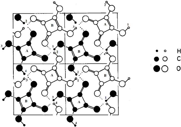
Figure 1: Crystal structure of squaric acid as viewed along the $b$ axis. Figure is taken from [21, 22]. Two adjacent layers are shown, with black and open circles each. The A and B type C₄O₄ groups are indicated (see text for explanation), and the hydrogen bonds are numbered.

As it is usual in the proton ordering models, we consider interactions between protons leading to an ordering in their system. Motion of protons in double-well potentials is described by pseudospins, whose two eigenvalues $\sigma=\pm 1$ are assigned to two equilibrium positions of the proton. We take into account the presence of the diagonal components of the lattice strain tensor $\varepsilon_{1}$, $\varepsilon_{2}$, and $\varepsilon_{3}$ that are induced via thermal expansion or by application of external hydrostatic pressure.

The system Hamiltonian in the case of squaric acid

$$H=U_{\textrm{seed}}+H_{\textrm{long}}^{\textrm{intra}}+H_{\textrm{long}}^{\textrm{inter}}+H_{\textrm{short}}$$ (1)

includes ferroelectric intralayer long-range interactions $H_{\textrm{long}}^{\textrm{intra}}$, ensuring ferroelectric ordering within each separate layer, antiferroelectric interlayer $H_{\textrm{ long}}^{\textrm{inter}}$ responsible for alternation of polarizations in the stacked layers, the short-range configurational interactions between protons $H_{\textrm{short}}$, and the so-called “seed” energy

$$U_{\textrm{seed}}=vN\left[\frac{1}{2}\sum_{ij=1}^{3}c_{ij}^{(0)}\varepsilon_{i}\varepsilon_{j}-\sum_{ij=1}^{3}c_{ij}^{(0)}\alpha_{i}^{(0)}(T-T_{i}^{0})\varepsilon_{j}\right],$$ (2)

containing elastic and thermal expansion contributions associated with uniform lattice strains; $c_{ij}^{(0)}$ are the corresponding “seed” elastic constants, whereas $\alpha_{i}^{(0)}$ are the “seed” thermal expansion coefficients. $T_{i}^{0}$ determines the reference point of the thermal expansion of the crystal, which can be chosen arbitrarily. $v$ is the unit cell volume, and $N$ is the number of the unit cells in the crystal. Such a form of (2) later on yields standard expressions for the strains of a stressed thermally expanding solid [see equation (25)].

The short-range Hamiltonian $H_{\textrm{short}}$ describes the four-particle confirational correlations between protons sitting around each C₄O₄ group. Similarly to how it is done for NH₄H₂PO₄, the antiferroelectrics of the KH₂PO$4$ type family, it is assumed that the energy of four lateral configurations $\varepsilon_{a}$ is the lowest of all, where two protons are in positions close to the adjacent oxygens of the C₄O₄ group, whereas two other protons are closer to the neighboring C₄O₄ groups (see figure 2). The next level is two diagonal configurations with the energy $\varepsilon_{s}$, where the protons are close to the opposite oxygens of the C₄O₄ group. Then, there are eight single-ionized configurations with three protons or only one close proton, having the energy $\varepsilon_{1}$, and two double-ionized configurations ($\varepsilon_{0}$) with four or no protons at all close to the given C₄O₄ group. It is believed that $\varepsilon_{a}<\varepsilon_{s}\ll\varepsilon_{1}\ll\varepsilon_{0}$.

If two protons are in the most energetically favorable lateral configurations, the C₄O₄ groups are isosceles trapezoids (point group C_1h), although very close to squares (C_4h). It is believed that this local distortion is caused by two single and two double alternating covalent bonds connecting the four oxygens to the carbons, and by formation of the double C–C bond within the C₄O₄ skeleton, as shown in figures 1 and 2. Double bonds are shorter than single ones between analogous atoms. Since the origin of the skeleton distortion is the chemical bonding with the local proton configuration, rather than macroscopic uniform lattice strains, all four lateral configurations still have the same energy of short-range interactions, no matter what their orientation relatively to the crystallographic axes is (see table 1). The same holds for the diagonal (point group C_2h), single-ionized (point group C₁), and double-ionized groups (point group D_2h). It means that no splitting of short-range energy levels by the macroscopic spontaneous strain takes place, in contrast to what was assumed in earlier theories for squaric acid [9] or for KH₂PO₄ type crystals [23, 24].

                    

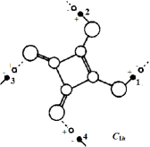
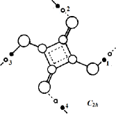
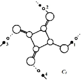
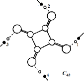
Figure 2: Lateral, diagonal, single and double ionized proton configurations around an A type C₄O₄ group in squaric acid. The hydrogen bonds $f=1,2,3,4$ are numbered. Two equilibrium positions of each proton are shown, and the signs $s_{f}=\pm 1$ of the eigenvalues of the $\sigma_{yqf}$ operators are indicated. Here $y$ stands for the layer index, $q$ is the index of the A type C₄O₄ group, and $f$ is the bond index.

Table 1: Proton configurations and their energies; $\varepsilon_{a}<\varepsilon_{s}\ll\varepsilon_{1}\ll\varepsilon_{0}$.

$i$		$s_{1}s_{2}s_{3}s_{4}$	${\cal E}_{i}$
1		$++--$	$\varepsilon_{a}$
2		$-++-$
3		$--++$
4		$+--+$
5		$-+-+$	$\varepsilon_{s}$
6		$+-+-$
15		$----$	$\varepsilon_{0}$
16		$++++$

$i$		$s_{1}s_{2}s_{3}s_{4}$	${\cal E}_{i}$
7		$+---$	$\varepsilon_{1}$
8		$-+--$
9		$--+-$
10		$---+$
11		$-+++$
12		$+-++$
13		$++-+$
14		$+++-$

To proceed from the representation of proton configuration energies to the pseudospin representation, we use a standard procedure, originally developed for the KH₂PO₄ type crystals [25, 26], where the Hamiltonian of the short-range correlations between protons, surrounding each A type C₄O₄ group is written as follows:

$$H_{yq}^{A}=\sum_{i=1}^{16}\hat{N}_{i}(yq){\cal E}_{i},\quad\hat{N}_{i}(yq)=\prod\limits_{f=1}^{4}\frac{1}{2}(1+s_{f}{\sigma}_{yqf})$$ (3)

where $\hat{N}_{i}(yq)$ is the operator of the four-particle configuration $i$; $s_{f}=\pm 1$ is the sign of the eigenvalue of the $\sigma_{yqf}$ operator in this particular configuration; ${\cal E}_{i}$ is the energy of the configuration. It is assumed that $s_{f}=+1$ if a proton at the $f$th bond is localized at the H-site proximal to the particular A type C₄O₄ group, and $s_{f}=-1$ if the proton is localized at the other (distal) H-site of the same bond. Using equation (3), we arrive at the following expression for the Hamiltonian

$$H_{yq}^{A}=V\left[\frac{\sigma_{yq1}}{2}\frac{\sigma_{yq2}}{2}+\frac{\sigma_{yq2}}{2}\frac{\sigma_{yq3}}{2}+\frac{\sigma_{yq3}}{2}\frac{\sigma_{yq4}}{2}+\frac{\sigma_{yq4}}{2}\frac{\sigma_{yq1}}{2}\right]$$

$$\quad{}+U\left[\frac{\sigma_{yq1}}{2}\frac{\sigma_{yq3}}{2}+\frac{\sigma_{yq2}}{2}\frac{\sigma_{yq4}}{2}\right]+\Phi\frac{\sigma_{yq1}}{2}\frac{\sigma_{yq2}}{2}\frac{\sigma_{yq3}}{2}\frac{\sigma_{yq4}}{2}.$$ (4)

The short-range interaction constants

$$V=-\frac{\varepsilon-w_{1}}{2},\quad U=\frac{\varepsilon+w_{1}}{2},\quad\Phi=2\varepsilon-8w+2w_{1},$$ (5)

are linear functions of the Slater-Takagi type energy parameters

$$\varepsilon=\varepsilon_{s}-\varepsilon_{a},\quad w=\varepsilon_{1}-\varepsilon_{a},\quad w_{1}=\varepsilon_{0}-\varepsilon_{a}.$$

Note that the model of non-interacting perpendicular one-dimensional chains is obtained from equation (18) at $\Phi=V=0$, i.e. at $\varepsilon=w_{1}=2w$, where the following order of the configuration energies should be assumed [13] $\varepsilon_{a}<\varepsilon_{1}<\varepsilon_{s}=\varepsilon_{0}$.

It can be shown, as it has been done for the KH₂PO₄ ferroelectrics, that the contributions of the correlations from the A and B type groups to the total thermodynamic potential are equal. The Hamiltonian of the short-range interactions in this case can be written as follows:

$$H_{\textrm{short}}\rightarrow 2\sum_{qy}H^{A}_{qy},$$ (6)

where the expression for $H^{A}_{qy}$ is given by equation (4).

The long-range interactions in the system Hamiltonian (1) are the dipole-dipole interactions, in analogy to the case of KH₂PO₄ [25], renormalized by the proton-lattice coupling. The MFA is successfully used for these interactions in the calculations for hydrogen-bonded ferroelectrics, if the fluctuations in the vicinity of the phase transition temperature neglected in this approximation are not the subject of special interest.

Within the MFA, we obtain the following expressions for the long-range intralayer

$$H_{\textrm{long}}^{\textrm{intra}}=-\frac{1}{2}\sum_{y=1}^{N_{y}}\sum_{qq^{\prime}\atop ff^{\prime}}J^{\textrm{intra}}_{ff^{\prime}}(qq^{\prime})\frac{\sigma_{yqf}}{2}\frac{\sigma_{yq^{\prime}f^{\prime}}}{2}\simeq-2\sum_{yqf}F_{yqf}^{\textrm{intra}}\frac{\sigma_{yqf}}{2}+\sum_{yqf}F_{yqf}^{\textrm{intra}}\frac{\langle\sigma_{yqf}\rangle}{2}$$ (7)

and for interlayer

$$H_{\textrm{long}}^{\textrm{inter}}=-\frac{1}{2}\sum_{y}\sum_{y^{\prime}\neq y}\sum_{qq^{\prime}\atop ff^{\prime}}J^{\textrm{inter}}_{ff^{\prime}}(yy^{\prime};qq^{\prime})\frac{\sigma_{yqf}}{2}\frac{\sigma_{y^{\prime}q^{\prime}f^{\prime}}}{2}\simeq-2\sum_{yqf}F_{yqf}^{\textrm{inter}}\frac{\sigma_{yqf}}{2}+\sum_{yqf}F_{yqf}^{\textrm{inter}}\frac{\langle\sigma_{yqf}\rangle}{2}$$ (8)

interactions. Here $N_{y}$ is the total number of the layers. The internal mean fields are as follows:

$$F_{yqf}^{\textrm{intra}}=\frac{1}{4}\sum_{q^{\prime}f^{\prime}}J^{\textrm{intra}}_{ff^{\prime}}(qq^{\prime})\langle\sigma_{yq^{\prime}f^{\prime}}\rangle,\quad F_{yqf}^{\textrm{inter}}=\frac{1}{4}\sum_{y^{\prime}q^{\prime}f^{\prime}}J^{\textrm{intra}}_{ff^{\prime}}(yy;qq^{\prime})\langle\sigma_{y^{\prime}q^{\prime}f^{\prime}}\rangle.$$ (9)

The following symmetry of the pseudospin mean values is assumed for the antiferroelectrically ordered two-sublattice model in the absence of external electric field

$$\langle\sigma_{yqf}\rangle=\exp[\mathrm{i}{\bf k}_{2}{\bf R}_{y}]\eta_{f}.$$ (10)

Here, ${\bf k}_{2}=(0,b_{2},0)$; $b_{2}$ is the basic vector of the reciprocal lattice; the factor $\exp[\mathrm{i}{\bf k}_{2}{\bf R}_{y}]=\pm 1$ denotes two sublattices of an antiferroelectric, ${\bf R}_{y}$ is the position vector of the $y$-th layer, and

$$\eta_{1}=-\eta_{3},\quad\eta_{2}=-\eta_{4},\quad\eta_{1}\approx\eta_{2}.$$ (11)

The last relation reflects the slight non-equivalence, mentioned in introduction, of hydrogen bonds, linking C₄O₄ groups along the $a$ and $c$ axes.

Even though each particular interaction parameter $J^{\textrm{intra}}_{ff^{\prime}}(qq^{\prime})$ and $J^{\textrm{inter}}_{ff^{\prime}}(yy^{\prime};qq^{\prime})$ is obviously changed by the strains $\varepsilon_{1}$ and $\varepsilon_{3}$, the symmetry of the long-range interaction matrices Fourier transforms

$$J^{\textrm{intra}}_{ff^{\prime}}(0)=\sum_{q^{\prime}}J^{\textrm{intra}}_{ff^{\prime}}(qq^{\prime}),\quad J^{\textrm{inter}}_{ff^{\prime}}({\bf k}_{2})=\sum_{q-q^{\prime}}\sum_{y-y^{\prime}}J^{\textrm{inter}}_{ff^{\prime}}(yy^{\prime};qq^{\prime})\exp[\mathrm{i}{\bf k}_{2}({\bf R}_{y}-{\bf R}_{y^{\prime}})]$$

over the bond indices $f$ and $f^{\prime}$, as can be easily checked, remains unchanged in the presence of the orthorhombic strain $\varepsilon_{1}-\varepsilon_{3}$:

$$J_{11}=J_{22}=J_{33}=J_{44},\quad J_{12}=J_{23}=J_{34}=J_{41},\quad J_{13}=J_{24}$$ (12)

both for $J^{\textrm{intra}}(0)$ and $J^{\textrm{inter}}_{ff^{\prime}}({\bf k}_{2})$. The symmetry (12) is obvious for strictly square-shaped C₄O₄ groups (point group C_4h). This is a statistically average symmetry of the paraelectric phase, where the hydrogens are placed, also statistically, in the middle of the hydrogen bonds.

Taking into account equations (10)–(12), we can write the Hamiltonians of the long-range interactions as follows:

$$H_{\textrm{long}}=H^{\textrm{intra}}_{\textrm{long}}+H^{\textrm{inter}}_{\textrm{long}}=N\nu[\eta_{1}^{2}+\eta_{2}^{2}]-2\nu\sum_{yq}\exp[\mathrm{i}{\bf k}_{2}{\bf R}_{y}]\left[\eta_{1}\frac{\sigma_{qy1}-\sigma_{qy3}}{2}+\eta_{2}\frac{\sigma_{qy2}-\sigma_{qy4}}{2}\right],$$ (13)

where

$$\nu=\nu^{\textrm{intra}}(0)+\nu^{\textrm{inter}}({\bf k}_{2})=\frac{J_{11}^{\textrm{intra}}(0)-J_{13}^{\textrm{intra}}(0)}{4}+\frac{J_{11}^{\textrm{inter}}({\bf k}_{2})-J_{13}^{\textrm{inter}}({\bf k}_{2})}{4}.$$ (14)

We also took into account the fact that $N_{y}N_{qA}=N$.

For the sake of simplicity, we shall hereafter neglect the weak non-equivalence of the perpendicular chains of hydrogen bonds and use a single order parameter

$$\eta\equiv\eta_{1}=\eta_{2}=-\eta_{3}=-\eta_{4}$$ (15)

instead of equation  (11).

The four-particle cluster approximation will be used for the short-range interactions, described by the Hamiltonian (4). With the long-range interactions taken into account in the mean field approximation, the thermodynamic potential of the system should be written as follows:

$$G = -vN\sum_{i=1}^{3}\sigma_{i}\varepsilon_{i}+NU_{\textrm{seed}}-\frac{1}{\beta}\sum_{qy}\left[2\ln\textrm{Sp}\exp(-\beta H_{qy}^{(4)})-\sum_{f=1}^{4}\ln\textrm{Sp}\exp(-\beta H_{qyf}^{(1)})\right]$$ (16)

$$+ \sum_{yqf}\left(F_{yqf}^{\textrm{intra}}+F_{yqf}^{\textrm{inter}}\right)\frac{\langle\sigma_{yqf}\rangle}{2}.$$

Here $\sigma_{1}=\sigma_{2}=\sigma_{3}=-p$, $\,\,\beta=(k_{\textrm{B}}T)^{-1}$, and

$$F_{yq1}^{\textrm{intra}}+F_{yq1}^{\textrm{inter}}=F_{yq2}^{\textrm{intra}}+F_{yq2}^{\textrm{inter}}=-F_{yq3}^{\textrm{intra}}-F_{yq3}^{\textrm{inter}}=-F_{yq4}^{\textrm{intra}}-F_{yq4}^{\textrm{inter}}=\exp[\mathrm{i}{\bf k}_{2}{\bf R}_{y}]\nu\eta.$$ (17)

The four-particle cluster Hamiltonian is

$$H_{qy}^{(4)}=H^{A}_{qy}-\sum_{f=1}^{4}\frac{z_{yqf}}{\beta}\frac{\sigma_{yqf}}{2}\,,$$ (18)

where

$$z_{yqf}=\beta(\Delta_{yqf}+2F_{yqf}^{\textrm{intra}}+2F_{yqf}^{\textrm{inter}}).$$

The fields $\Delta_{yqf}$ are the effective cluster fields that describe short-range interactions of the spin $\sigma_{yqf}$ with the particles from outside the cluster $q$. They are determined from the self-consistency condition stating that pseudospin mean values calculated with the four-particle (18) and with the one-particle

$$H^{(1)}_{yqf}=-\left[{2\Delta_{yqf}+2F_{yqf}^{\textrm{intra}}+2F_{yqf}^{\textrm{inter}}}{}\right]\frac{\sigma_{yqf}}{2}$$

Hamiltonians should coincide. We get

$$z_{yq1}=z_{yq2}=-z_{yq3}=-z_{yq4}=\exp[\mathrm{i}{\bf k}_{2}{\bf R}_{y}]z\,,\quad z=\frac{1}{2}\ln\frac{1+\eta}{1-\eta}+\beta\nu\eta.$$ (19)

Taking into account equations (13), (15), (18), (19), the thermodynamic potential per one unit cell is obtained in the following form

$$g=U_{\textrm{seed}}-\frac{2}{\beta}\left[\ln D+\ln(1-\eta^{2})\right]+2\nu\eta^{2}-v\sum_{i=1}^{3}\sigma_{i}\varepsilon_{i}\,,$$ (20)

where

$$D=a+\cosh 2z+4b\cosh z+1,\quad a=\exp(-\beta\varepsilon),\quad b=\exp(-\beta w).$$

In the earlier theories [18, 27], the short-range Slater-Takagi energies in the KH₂PO₄ family crystals were considered as quadratic functions of the distance $\delta$. For the squaric acid, we shall employ the same scheme. Using the term of the relative deviation of $\delta$ from its value $\delta_{0}$ at ambient pressure (we shall call it a displacement $\mu^{\prime}$)

$$\mu^{\prime}=\frac{\delta-\delta_{0}}{\delta_{0}}\,,$$ (21)

we assume that

$$\varepsilon=\varepsilon_{0}(1+\mu^{\prime})^{2}\,,\quad w=w_{0}(1+\mu^{\prime})^{2}\,.$$ (22)

Here, the quadratic in $\mu^{\prime}$ terms, omitted in [18], are included into consideration.

For the parameter of long-range (dipole-dipole) interactions $\nu$, we take into account both the dependence of the dipole moments on $\delta$ and the changes in the interaction parameter due to the overall crystal deformation [18] and associated with changes in the equilibrium distances between protons (dipoles)

$$\nu=\nu_{0}(1+\mu^{\prime})^{2}+\sum_{i=1}^{3}\psi_{i}\varepsilon_{i}.$$ (23)

It should be underlined that none of the earlier theories [18, 27] described the thermal expansion of the crystals; therefore, the deformational effects there were only those caused by external pressures. On the contrary, in the present model the strains $\varepsilon_{i}$ are induced both by temperature changes and by external pressures. In the mean field approximation, the expansion (23) gives rise to the terms of electrostriction type in the Hamiltonian, linear in the strains and quadratic in the sublattice polarization (order parameter $\eta$).

In [18, 27], the distance $\delta$ was treated as a pressure dependent and temperature independent model parameter, with the linear pressure dependence chosen either from the available experimental data or by fitting the theory to experiment for the transition temperatures. In the present work, we shall use a similar approach and assume $\delta$ to vary according to its experimentally observed above the transition linear temperature [1] and external hydrostatic pressure $p$ [17] dependences

$$\delta=\delta_{0}[1+\delta_{p}p+\delta_{T}(T-T_{\textrm{N0}})],$$ (24)

where $T_{\textrm{N}0}$ is the transition temperature at ambient pressure. It means that the anomalous temperature behavior of $\delta$ below the transition point and its jump at $T_{\textrm{N}}$ are neglected.

Minimization of the thermodynamic potential (20) with respect to the order parameter $\eta$ and strains $\varepsilon_{i}$

$$\frac{\partial g}{\partial\eta}=0,\quad\frac{\partial g}{\partial\varepsilon_{i}}=0$$

yields the following equations

$$\eta=\frac{\sinh 2z+2b\sinh z}{D},$$

$$\sigma_{i}=\sum_{j=1}^{3}c_{ij}^{(0)}\varepsilon_{j}-\sum_{j=1}^{3}c_{ij}^{(0)}\alpha_{j}^{(0)}(T-T_{j}^{0})+\frac{2\psi_{i}\eta}{v}\left(\eta-2\frac{\sinh 2z+2b\sinh z}{D}\right).$$

From the above it follows that in equilibrium

$$\varepsilon_{k}=\alpha_{k}^{(0)}(T-T_{k}^{0})+\sum_{i=1}^{3}\sigma_{i}s_{ki}^{(0)}-\frac{2\eta^{2}}{v}\sum_{i=1}^{3}\psi_{i}s_{ki}^{(0)},$$ (25)

where $s_{ki}^{(0)}$ is the matrix of “seed” elastic compliances, inverse to $c_{ij}^{(0)}$. One can see that in the paraelectric phase ($\eta=0$), the microscopic contributions to the strains vanish, whereas in the ordered phase they are proportional to $\eta^{2}$, indicating the electrostriction type contributions governed by the parameters $\psi_{i}$.

Finally, the molar entropy of the proton subsystem is as follows:

$$\Delta S=\ln[(1-\eta^{2})D]-\frac{1}{DT}\left[a\varepsilon+4bw\cosh z\right]-2\frac{\nu\eta^{2}}{T}.$$ (26)

3 Calculations

In the calculations, the thermodynamic potential is minimized numerically with respect to the order parameter $\eta$. At the same time, the strains $\varepsilon_{i}$ are determined from equation (25).

The quantities that should be described include:
the temperature curves at ambient pressure of

• the sublattice polarization (order) parameter,

• macroscopic lattice strains $\varepsilon_{i}$,

• thermal expansion coefficients and specific heat;

the pressure curves of

• the transition temperature $T_{\textrm{N}}$,

• lattice strains $\varepsilon_{i}$.

Since we do not want to overcomplicate the fitting procedure by adopting different values of the model parameters for paraelectric and antiferroelectric phase, the chosen matrix quantities $c_{ij}^{(0)}$, $\alpha_{i}^{(0)}$, $T_{i}^{0}$ should obey the tetragonal symmetry of paraelectric phase, namely $c_{11}^{(0)}=c_{33}^{(0)}$, $c_{12}^{(0)}=c_{23}^{(0)}$, $\alpha_{1}^{(0)}=\alpha_{3}^{(0)}$, $T_{1}^{0}=T_{3}^{0}$.

There are four different “seed” elastic constants $c_{11}^{(0)}$, $c_{22}^{(0)}$, $c_{12}^{(0)}$, and $c_{13}^{(0)}$. We take $c_{11}^{(0)}$ to be equal to the experimental value of $c_{11}$ [28] above the transition point. Experimental elastic constant $c_{22}$ was found to slightly decrease with an increasing temperature [28, 29]. The “seed” $c_{22}^{(0)}$ is chosen accordingly, coinciding with the data of [28]. Finally, $c_{12}^{(0)}$ and $c_{13}^{(0)}$, for which no convincing experimental data are available, were chosen to provide a correct fit to the experimental [30] pressure dependence of the lattice constants $a$ and $b$ at 292 K.

The parameters of the short-range correlations $\varepsilon_{0}$ and $w_{0}$ govern the temperature behavior of the order parameter $\eta$ (in particular, the magnitude of its jump at the transition $\Delta\eta_{c}$ and steepness of its rise to saturation with lowering temperature) and the value of the transition temperature at ambient pressure $T_{\textrm{N}0}$. The latter is also extremely sensitive to the value of the long-range interactions parameter $\nu_{0}$. Hence, the set of $\varepsilon_{0}$, $w_{0}$, and $\nu_{0}$ is chosen to yield $T_{\textrm{N}0}=373.5$ K, $\Delta\eta_{c}\approx 0.57$, as well as a correct temperature curve of $\eta$ between the transition and saturation. Contributions of the double-ionized configurations are neglected by putting $w_{1}\to\infty$.

The “seed” thermal expansion coefficients $\alpha_{i}^{(0)}$ as well as the parameters $\psi_{i}$ are determined by fitting the theoretical temperature dependences of the lattice strains to experimental data [5, 31]. In fact, $\alpha_{i}^{(0)}$ should be simply equal to the corresponding paraelectric experimental values, as is seen directly in equation (25). The parameters $\psi_{i}$, on the other hand, are unambiguously determined by fitting the calculated anomalous parts of the strains to the experiment below the transition temperature, using the same equation (25). As $\psi_{i}$ are relevant for the ordered phase only, they do not have to adhere to the symmetry of the paraelectric phase; hence, we can take $\psi_{1}\neq\psi_{3}$, as is indeed required by the just described fitting.

As we have already mentioned, the temperatures $T_{i}^{0}$ determine the reference point of the thermal expansion of the crystal, which can be set arbitrarily. Thus, $T_{i}^{0}$ are not fitting parameters of the model and, therefore, can also be chosen arbitrarily. In our calculations we chose them to yield zero values of the lattice strains $\varepsilon_{i}$ just above the transition temperature at ambient pressure. In fact, $T_{1}^{0}=T_{2}^{0}=T_{\textrm{N}0}=373.5$ K, as seen from equation (25).

As already described, we take $\delta$ to vary according to its experimentally observed linear temperature and external hydrostatic pressure (24). The coefficients $\delta_{T}$ and $\delta_{p}$ are deduced from the data of [1] and [17].

The unit cell volume is $v=2\cdot 10^{-28}$ m³ just above the transition point at ambient pressure, as determined from the data of [5]. The final values of the model parameters, used in our calculations, are given in table 2.

Table 2: The adopted values of the model parameters.

$\varepsilon_{0}/k_{\text{B}}$

$w_{0}/k_{\text{B}}$

$\nu_{0}/k_{\text{B}}$

$\psi_{1}/k_{\text{B}}$

$\psi_{2}/k_{\text{B}}$

$\psi_{3}/k_{\text{B}}$

$\alpha_{1}^{0}$

$\alpha_{2}^{0}$

$\delta_{T}$

$\delta_{p}$

$c_{11}^{0}$

$c_{12}^{0}$

$c_{13}^{0}$

$c_{22}^{0}$

K

$10^{-5}$ K-1

$10^{-4}$ K-1

kbar-1

$10^{10}$ N/m2

395

1100

79.8

$-518$

445

1096

1.2

13.0

2

$-0.014$

6.5

2.3

$-3.1$

$2.38{-}0.02T$

In figure 3 we show the calculated temperature dependence of the order parameter $\eta$ and the spontaneous strain $\varepsilon_{1}-\varepsilon_{3}$ at ambient pressure. Experimental points for $\eta$ were obtained from the ¹³C NMR measurements. A clear first order phase transition is observed, with the jump of the order parameter $\Delta\eta_{c}\simeq 0.57$. The spontaneous strain $\varepsilon_{1}-\varepsilon_{3}$ is negative below the transition and, as it follows from equation (25), it is proportional to the square of the order parameter $\eta^{2}$.

       

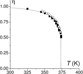
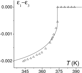
Figure 3: Temperature dependence of the order parameter and spontaneous strain $\varepsilon_{1}-\varepsilon_{3}$ of squaric acid. Lines: the theory; symbols are experimental points taken from [6] ($\blacksquare$), [32] ($\bigcirc$), and [5] ($\bigtriangleup$).

The temperature dependences of the diagonal lattice strains $\varepsilon_{i}$ and the corresponding thermal expansion coefficients are shown in figure 4. The coefficients were calculated by numerical differentiation of the strains with respect to temperature.

       

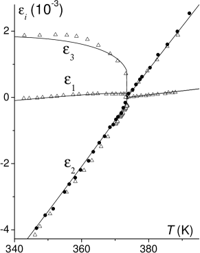
Figure 4: Temperature dependences of the macroscopic lattice strains and of the corresponding thermal expansion coefficients of squaric acid at ambient pressure. Lines: the theory; symbols are experimental points taken from [5] ($\bigtriangleup$) and [31] ($\bullet$).

A clear anisotropy of the thermoelastic properties of squaric acid within the $ac$ plane and in the perpendicular direction is seen. At temperature lowering, the strain $\varepsilon_{2}$ has a downward jump at the transition and a negative anomalous part in the ordered phase. The strains $\varepsilon_{1}$ and $\varepsilon_{3}$, on the other hand, have upward jumps and positive anomalous parts. As is shown above [see equation (25)], the anomalous contributions to the macroscopic strains are strictly proportional to the square of the order parameter $\eta^{2}$. The thermal expansion coefficients $\alpha_{1}=\alpha_{3}$ in the paraelectric phase are by one order of magnitude smaller than $\alpha_{2}$; their anomalies at the transition point are of different signs.

The specific heat of the proton subsystem is calculated by numerical differentiation of the entropy (26) with respect to temperature

$$\Delta C_{p}=-\frac{T}{M}\left(\frac{\partial\Delta S}{\partial T}\right)_{p},$$

where $M=114.06$ g/mol is the molar mass of squaric acid. The corresponding temperature curve is given in figure 5. The experimental points for the anomalous part of the specific heat are obtained by subtracting the regular part, best described as a slightly non-linear curve $C_{\text{reg}}=-0.48803+0.00738T-7.3\cdot 10^{-6}T^{2}$ (J/g K), from the total specific heat as it was measured in [33]. One can see that a satisfactory agreement with experiment is obtained, even though the specific heat was not directly involved in the above described fitting procedure.

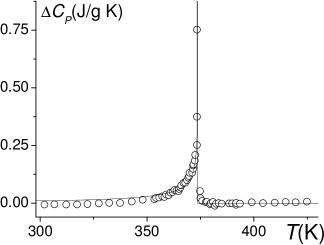
Figure 5: Temperature dependence of the specific heat of squaric acid. Line: the theory; symbols are experimental points derived from the data of [33] as described in text.

The calculated hydrostatic pressure dependences of the paraelectric lattice constants are shown in figure 6. The lattice constants were determined as $a=a_{0}[1+\varepsilon(1)]$, $b=b_{0}[1+\varepsilon(2)]$, where $a_{0}=6.137$ Å, $b_{0}=5.327$ Å are the values of the lattice constants just above the transition point at ambient pressure [5]. A good agreement with experiment is obtained.

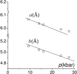
Figure 6: Lattice constants at 292 K as functions of hydrostatic pressure. Lines: the theory; symbols are experimental points taken from [30].

In figure 7 we plot the hydrostatic pressure dependence of the phase transition temperature in squaric acid. As expected, the calculated transition temperature decreases with pressure (the dashed line). Quantitatively, however, completely non-satisfactory results are obtained. With the pressure variation of $\mu^{\prime}$ as observed experimentally [17] and the parameters $\psi_{i}$ determined by fitting to the lattice strains below transition at ambient pressure, the rate, with which the calculated transition temperature decreases with hydrostatic pressure, $\partial T_{c}/\partial p=-19.5$ K/kbar, is nearly twice as large as the experimental one. The observed disagreement means, foremost, that equation (23) yields a too fast decrease of the long-range interaction parameter $\nu$, to which the theoretical values of the transition temperature are most sensitive. The pressure variation of the Slater-Takagi energies is less important here.

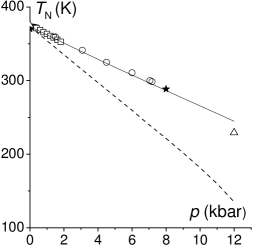
Figure 7: Transition temperature of squaric acid as a function of hydrostatic pressure. Symbols are experimental points taken from [8] ($\square$), [7] ($\circ$), [4] ($\bigtriangledown$) and [17] ($\star$). The dashed and solid lines: the theory, calculated with equations (22), (23) and with equations (27), (28), respectively.

Below we discuss a possible origin of the model inconsistency and ways to solve this problem. To this end, let us look closely at the obtained pressure dependence of $\nu$.

It is expected that the term $\sum_{i}\psi_{i}\varepsilon_{i}$ in presence of high hydrostatic pressure would be positive, thereby leading to an increase of the long-range interaction parameter $\nu$ due to the reduction of the average interparticle distances in the compressed crystal. However, when the values of the parameters $\psi_{i}$ are chosen to fit to the experimental data [5] for the anomalous spontaneous temperature behavior of the strains $\varepsilon_{i}$ below the transition at ambient pressure, the sum $\sum_{i}\psi_{i}\varepsilon_{i}$ in presence of high pressure becomes negative, not slowing, as expected, but enhancing the decrease of $\nu$ caused by the decrease of the H-site distance $\delta$. Of course, one cannot exclude a possibility that further measurements may yield the values of the strains $\varepsilon_{1}(T)$, $\varepsilon_{3}(T)$ different from those obtained in [5] and unconfirmed yet by other measurements. The reasoning below, however, is based on the assumption that the data of [5] are correct.

An obvious workaround but rather clumsy way to obtain the necessary pressure dependence of $\nu$ is to assume that there are some other high-pressure factors, not included into (22) and (23), and to include them empirically via the terms $k_{p}p$, namely

$$\varepsilon=\varepsilon_{0}\left[(1+\mu^{\prime})^{2}+k_{p1}p\right],\quad w=w_{0}\left[(1+\mu^{\prime})^{2}+k_{p1}p\right],$$ (27)

and

$$\nu=\nu_{0}\left[(1+\mu^{\prime})^{2}+k_{p2}p\right]+\sum_{i=1}^{3}\psi_{i}\varepsilon_{i}.$$ (28)

We can speculate, for instance, that external pressure causes a redistribution of electron density, thereby changing the effective charges of the ions and, as a result, chanding the interactions between them. Introduction of two extra fitting parameters $k_{p1}$ and $k_{p2}$ indeed allows us to describe the pressure variation of the transition temperature (see figure 6, the solid line). At $k_{p1}=k_{p2}=0.0151$ kbar^-1 we obtain $\partial T_{c}/\partial p=-10.7$ K/kbar, in total agreement with experiment. Other combinations of $k_{p1}$ and $k_{p2}$ values can be found, also yielding the desired fit for the $T_{c}$ vs $p$ dependence. Accepting this, the already obtained good agreement with experiment for the system behavior at ambient pressure is not affected.

4 Conclusions

We present a modification to the proton ordering model, aimed at describing the effects associated with diagonal lattice strains in H-bonded antiferroelectric crystals of squaric acid. These effects include thermal expansion of the crystals, the appearance of spontaneous strain $\varepsilon_{1}-\varepsilon_{3}$ below the phase transition, and the shift of the transition temperature with hydrostatic pressure. Here, both the macroscopic lattice strains and the changes in the local geometry of hydrogen bonds are found to be essential. As usually, the quadratic dependence of the parameters of short-range and long-range interactions between protons on the H-site distance $\delta$ is assumed.

The deformational phenomena at ambient pressure are well described by the developed theory. On the other hand, the experimental dependence of the transition temperature on hydrostatic pressure can be described only if we assume that there are additional mechanisms to the pressure dependence of the interaction constants of the model, other than via the electrostriction interactions with the diagonal macroscopic strains and via the shortening of $\delta$, or if we suggest a further modification of the model, in which $\delta$ would be considered as an independent thermodynamic variable.

Ukrainian 0

Åôåêòè, ïîâ’ÿçàíi ç äiàãîíàëüíèìè äåôîðìàöiÿìè òà ãåîìåòðiєþ âîäíåâèõ çâ’ÿçêiâ, â àíòèñåãíåòîåëåêòðèчíèõ êðèñòàëàõ êâàäðàòíî¿ êèñëîòè À.Ï. Ìî¿íà

             
Iíñòèòóò ôiçèêè êîíäåíñîâàíèõ ñèñòåì ÍÀÍ Óêðà¿íè, âóë. Ñâєíöiöüêîãî, 1, 79011 Ëüâiâ, Óêðà¿íà

References

-
[1]
Semmingsen D., Tun Z., Nelmes R.J., McMullan R.K., Koetzle T.F., Z. Kristallogr., 1995, 210,
934–947, doi:10.1524/zkri.1995.210.12.934. - [2] Semmingsen D., Hollander F.J., Koetzle T.F., J. Chem. Phys., 1977, 66, 4405–4412, doi:10.1063/1.433745
- [3] Hollander F.J., Semmingsen D., Koetzle T.F., J. Chem. Phys., 1977, 67, 4825–4831. doi:10.1063/1.434686.
-
[4]
Moritomo Y., Tokura Y., Takahashi H., Mōri N., Phys. Rev. Lett., 1991, 67, 2041-2044,
doi:10.1103/PhysRevLett.67.2041. - [5] Ehses K.H., Ferroelectrics, 1990, 108, 277–282, doi:10.1080/00150199008018770.
- [6] Klymachyov A.N., Dalal, N.S., Z. Phys. B: Condens. Matter, 1997, 104, 651–656, doi:10.1007/s002570050503.
- [7] Samara G.A., Semmingsen D., J. Chem. Phys., 1979, 71, 1401–1407, doi:/10.1063/1.438442.
- [8] Yasuda N., Sumi K., Shimizu H., Fujimoto S., Okada K., Suzuki I., Sugie H., Yoshino K., Inuishi Y., J. Phys. C: Solid State Phys., 1978, 11, L299–L303, doi:10.1088/0022-3719/11/8/002.
- [9] Matsushita E., Matsubara T., Progr. Theor. Phys., 1980, 64, No. 4, 1176–1192, doi:10.1143/PTP.64.1176.
- [10] Matsushita E., Matsubara T., Ferroelectrics, 1981, 39, 1095–1098, doi:10.1080/00150198108219573.
- [11] Matsushita E., Matsubara T., Progr. Theor. Phys., 1982, 68, No. 6, 1811–1826, doi:10.1143/PTP.68.1811.
- [12] Chaudhuri B.K., Dey P.K., Matsuo T., Phys. Rev. B, 1990, 41, 2479–2489, doi:10.1103/PhysRevB.41.2479.
-
[13]
Maier H.-D., Müser H.E., Petersson J., Z. Phys. B: Condens. Matter, 1982, 46, 251–260,
doi:10.1007/BF01360302. -
[14]
Deininghaus U., Mehring M., Solid State Commun., 1981, 39, No. 11, 1257–1260,
doi:10.1016/0038-1098(81)91126-1 -
[15]
Ishizuka H., Motome Y., Furukawa N., Suzuki S.,
Phys. Rev. B, 2011, 84, 064120 (6 pages),
doi:10.1103/PhysRevB.84.064120. - [16] Vijigiri V., Mandal S., J. Phys.: Condens. Matter, 2020, 32, 285802, doi:10.1088/1361-648X/ab7ba1.
- [17] Mcmahon M.I., Piltz R.O., Nelmes R.J., Ferroelectrics, 1990, 108, 277–282, doi:10.1080/00150199008018770.
- [18] Stasyuk I.V., Levitskii R.R., Moina A.P., Phys. Rev. B, 1999, 59, 8530–8540, doi:10.1103/PhysRevB.59.8530.
-
[19]
Moina A.P., Levitskii R.R., Zachek I.R., Condens. Matter Phys., 2011, 14, 43602 (18 pages),
doi:10.5488/CMP.14.43602. - [20] Blinc R., Zeks B., Ferroelectrics, 1987, 72, 193–227, doi:10.1080/00150198708017947.
- [21] Semmingsen D., Feder J., Solid State Commun., 1974, 15, 1369–1372, doi:10.1016/0038-1098(74)91382-9.
- [22] Moritomo Y., Koshihara S., Tokura Y., J. Chem. Phys., 1990, 93, 5429–5435, doi:10.1063/1.459639.
-
[23]
Stasyuk I.V., Levitskii R.R., Zachek I.R., Moina A.P., Phys. Rev. B, 2000, 62, 6198–6207,
doi:10.1103/PhysRevB.62.6198. -
[24]
Stasyuk I.V., Levitskii R.R., Moina A.P., Lisnii B.M., Ferroelectrics, 2001, 254, 213–227,
doi:10.1080/00150190108215002. - [25] Blinc R., Svetina S., Phys. Rev., 1966, 147, 430–438, doi:10.1103/PhysRev.147.430.
- [26] Levitskii R.R., Lisnii B.M., Phys. Status Solidi B, 2004, 241, 1350–1368, doi:10.1002/pssb.200301995.
- [27] Torstveit S., Phys. Rev. B, 1979, 20, 4431–4441, doi:10.1103/PhysRevB.20.4431.
- [28] Rehwald W., Vonlanthen A., Phys. Status Solidi B, 1978, 90, 61–66 doi:10.1002/pssb.2220900106.
- [29] Yamanaka A., Tatsuzaki I., J. Phys. Soc. Jpn., 1987, 56, 1043–1050, doi:10.1143/JPSJ.56.1043.
-
[30]
Katrusiak A., Nelmes R.J., J. Phys. C: Solid State Phys., 1986, 19, L765–L772,
doi:10.1088/0022-3719/19/32/001. - [31] Johansen T. H., Feder J., Jøssang T., Z. Phys. B: Condens. Matter, 1984, 56, 41–49, doi:10.1007/BF01470211.
- [32] Mehring M., Becker J.D., Phys. Rev. Lett., 1981, 47, 366–370, doi:10.1103/PhysRevLett.47.366.
- [33] Barth E., Helwig J., Maier H.-D., Müser H.E., Petersson J., Z. Phys. B: Condens. Matter, 1979, 34, 393–397, doi:10.1007/BF01325204.
Ukrainian \adddialect\l@ukrainian0 \l@ukrainian