Thermodynamics, shadow and quasinormal modes of black holes
in five-dimensional Yang-Mills massive gravity

Abstract

In this paper, we consider the Einstein-massive gravity coupled to the Yang-Mills gauge field in five dimensions. Concentrating on the static solutions with planar horizon geometry, we explore the thermodynamic behavior in the extended phase space and examine the validity of the first law of thermodynamics besides local thermal stability by the Hessian matrix. We observe that although the topology of boundary is planar, there exists the van der Waals like phase transition for this kind of solution. We find the critical quantities and discuss how the massive and Yang-Mills parameters affect them. Furthermore, some signatures of the first order phase transition such as the swallow-tail behavior of the Gibbs free energy and divergencies of the specific heat are given in detail. We continue with the calculation of the photon sphere and the shadow observed by a distant observer. Finally, we use the WKB method to investigate the quasinormal modes for scalar perturbation under changing the massive and Yang-Mills parameters.

I Introduction

One of the interesting predictions of general relativity is the existence of black holes which are the most mysterious objects in the Universe. Although it is believed that black holes are invisible, it is possible to have an image of them; which has been captured by the Event Horizon Telescope Akiyama:2019cqa . The image of a supermassive black hole in the galaxy $M87$, a dark part which is surrounded by a bright ring, was the first direct evidence of the existence of black holes consistent with the prediction of general relativity. What makes it possible is bending the light of luminous sources behind the black hole or emitting radiation from matter plunging into the black hole. In spite of the fact that gravitational lensing (bending of light rays by spacetime curvature) is crucial, the existence of unstable photon orbits makes it possible that photons in the vicinity of a black hole escape from gravity to a distant observer, where they form a bright ring around the black shadow (for a recent review see Dokuchaev:2019jqq ).

Black hole’s shadow, as an important observable, has become the subject of interest, thereby we can extract information about the parameters of a black hole and its near geometry Bambi:2019tjh . Moreover, the shadow image measurements can determine whether Einstein’s general relativity is correct or whether it should be modified in the presence of strong gravitational fields Moffat:2015kva . One of the goals of this paper is to explore the shadow of the $5-$dimensional massive-Yang-Mills black hole and study the effect of different parameters on the size of photon orbits and spherical shadow.

Black holes are interacting with the matters and radiations in surroundings. The gravitational waves are the signals of black holes in reaction to these perturbations GW . The dominant part of such signals are quasinormal modes which are damping oscillations after the initial outbursts of radiation and they end to the late-time tails after a very long time. The gravitational quasinormal modes can determine if the black hole is stable and thus may exist in nature. On the other hand, quasinormal modes are connecting with the thermodynamic phase transition in the dual field theory according to the AdS/CFT correspondence and the hydrodynamic regime of strongly coupled field theories (for a detailed discussion see Konoplya:2011qq ). So we are motivated to investigate quasinormal modes for the considered black hole. For some works calculating quasinormal modes for solutions of dRGT massive gravity in four dimensions see Ponglertsakul:2018smo ; Hendi:2018hdo ; Moulin:2019ekf ; Zou:2017juz ; Burikham:2017gdm ; Chen:2019kaq ; Prasia:2016fcc .

In the path of finding new physics, black holes play an essential role. Among the huge range of studies about the different aspects of these objects, observing similarity with the everyday thermodynamics is certainly astonishing Kubiznak:2016qmn . As an interesting similarity, one may find a van der Waals like behavior for spherically symmetric charged AdS black holes Kubiznak:2016qmn . This becomes possible with changing the role of black hole mass and defining a thermodynamic pressure term proportional to the cosmological constant. Correspondence between the black hole parameters and the fluid thermodynamic quantities, in this perspective, gives rise to a new picture of black holes called black hole chemistry. While the small-large black hole phase transition now mimics the role of liquid-gas phase transition. Regarding the thermodynamic pressure with thermodynamic volume as its conjugate quantity guides us towards the generalized first law in the extended phase space thermodynamics. Investigation of thermodynamic phase transition in the context of alternative theories of gravity is interesting, since one may encounter a new phenomenon which is not observed in Einstein gravity (for example see Hendi:2017fxp ).

One of the highly successful extensions of the Einstein gravity is dRGT massive gravity deRham:2010ik . This theory introduces a novel potential term by the contribution of some polynomial interactions and a reference metric which may lead to the mass term for the graviton. This version of massive gravity gives unique features to the theory and avoids the common instabilities observed in other theories with a massive spin-$2$ field in their spectrum deRham:2010kj ; deRham:2014zqa . The very basic question that how the existence of mass for the graviton affects the thermodynamic behavior of black holes has been explored in the literature (see for e.g. Hendi:2017fxp ; Cai:2014znn ; Hendi:2015eca ; Ghosh:2015cva ; Hendi:2016vux ; Zou:2016sab and references therein). In this paper, we also consider black hole solutions of the dRGT massive gravity coupled with the Yang-Mills field and investigate their thermodynamics.

One of the interesting ways for coupling matter to the gravity theory is using the non-abelian Yang-Mills gauge field. Criticality and possibility of phase transition have been discussed for black holes in the theories AdS-Maxwell-power-Yang-Mills Zhang:2014eap ; ElMoumni:2018fml , Einstein-Born-Infeld-Yang-Mills Meng:2017srs , $f(R)$ gravity coupled with Yang-Mills field Ovgun:2017bgx , Gauss-Bonnet massive gravity coupled to Maxwell and Yang-Mills fields Meng:2016its and Wu-Yang model of Yang-Mills massive gravity in the presence of Born-Infeld nonlinear electrodynamics Hendi:2018hdo .

Black hole thermodynamics may have different behavior in higher dimensions. As an example, it was shown that Hendi-Dehghani for charged topological black holes in the grand canonical ensemble, the van der Waals like phase transition could take place only for $dimensions\geq 5$. The five-dimensional spacetime is important for different aspects; from its verification as a candidate for unifying electromagnetic and gravity forces to appearing black hole solutions with different horizon topologies Horowitz:2012nnc ; Wesson:2014raa .

In this paper, we focus on the Einstein-Massive gravity in the presence of the Yang-Mills gauge field in $5$-dimensions. Recently, the static solutions with the planar horizon for this theory have been introduced in Ref. Sadeghi:2018ylh . We are interested to discuss the thermodynamic aspects of these solutions in the extended phase space thermodynamics and looking for the possible van der Waals like phase transition. Furthermore, we investigate the possibilities for the formation of shadow and variation of its size under considering different parameters. At last, we calculate frequencies of quasinormal modes for scalar perturbations by using the WKB method.

The plan of the paper is as follows: In Sec. II, we give a brief review of the action with the planar AdS solutions. Then, we obtain the thermodynamic quantities. Investigation of the critical behavior and the van der Waals phase transition, as well as studying the effects of both massive and Yang-Mills parameters on the critical quantities are addressed in Sec. III. Next, the consistency of local thermal stability conditions in two canonical and grand canonical ensembles is discussed. Moreover, it is shown that the first law is valid for the kind of considered solutions. We also explore the photon orbits near the black hole and formation of shadow in Sec. IV. In the last section V, the quasinormal modes for scalar perturbation are presented. Finally, we give the concluding remarks in Sec. VI.

II Action and thermodynamics

The action of $5-$dimensional Einstein-massive gravity with negative cosmological constant in the presence of Yang-Mills source is as follows

$$S=\int d^{5}x\sqrt{-g}\left(R-2\Lambda-F^{(a)}_{\mu\nu}F^{(a)\mu\nu}+m^{2}\sum_{i=1}^{3}c_{i}\mathcal{U}_{i}(g,f)\right),$$ (1)

where $R$ and $\Lambda$ are, respectively, the scalar curvature and the negative cosmological constant. The Yang-Mills tensor $F^{(a)}_{\mu\nu}$ is

$$F^{(a)}_{\mu\nu}=\partial_{\mu}A_{\nu}-\partial_{\nu}A_{\mu}+\frac{1}{2e}f_{(b)(c)}^{(a)}A_{\mu}^{(b)}A_{\nu}^{(c)},$$ (2)

where $e$ is the gauge coupling constant and $A_{\mu}^{(a)}$ is the gauge potential. The $f_{(b)(c)}^{(a)}$ are gauge group structure constants and for the $SU(N)$ group, one has $a,b,c=1...N^{2}-1$. Regarding the last term of the action (massive term), $c_{i}$’s are some constants and $\mathcal{U}_{i}$’s are symmetric polynomials of the eigenvalues of $\mathcal{K}^{\mu}_{\nu}=\sqrt{g^{\mu\alpha}f_{\alpha\nu}}$ with the following explicit forms

$$\mathcal{U}_{1}=[\mathcal{K}],$$ (3)

$$\mathcal{U}_{2}=[\mathcal{K}]^{2}-[\mathcal{K}^{2}],$$

$$\mathcal{U}_{3}=[\mathcal{K}]^{3}-3[\mathcal{K}][\mathcal{K}^{2}]+2[\mathcal{K}^{3}].$$

We follow the reference metric ansatz $f_{\mu\nu}=(0,0,c_{0}^{2}h_{ij})$ with positive constant $c_{0}$ and $h_{ij}=\frac{1}{b^{2}}\delta_{ij}$, where “$b$” is an arbitrary constant with dimension of length. Hereafter, we follow the metric solution of the five-dimensional planar AdS black brane introduced in Ref. Sadeghi:2018ylh

$$ds^{2}=-f(r)dt^{2}+\frac{dr^{2}}{f(r)}+r^{2}h_{ij}dx^{i}dx^{j},$$ (4)

where by introducing notation $\mathtt{C}_{i}=m^{2}c_{0}^{i}c_{i}$ with $i=1,2,3$, the blackening factor with the horizon radius $r_{+}$ and $AdS$ radius $\ell=\sqrt{-6/\Lambda}$ is

$$f(r) = \frac{1}{r^{2}}\left[\frac{r^{4}-r_{+}^{4}}{\ell^{2}}+\frac{\mathtt{C}_{1}}{3}(r^{3}-r_{+}^{3})+\mathtt{C}_{2}(r^{2}-r_{+}^{2})\right.$$ (5)

$$+\left.2\mathtt{C}_{3}(r-r_{+})-2e^{2}\ln(\frac{r}{r_{+}})\right].$$

As we expect, in the limit of vanishing parameters for massive and Yang-Mills terms, the familiar form of metric function $f(r)=\frac{r^{2}}{\ell^{2}}-\frac{r_{+}^{4}}{r^{2}\ell^{2}}$ for the $5$-dimensional planar AdS spacetime is recovered.

Considering Eq. (4), we can compute the Kretschmann scalar

$$R_{\alpha\beta\gamma\delta}R^{\alpha\beta\gamma\delta}=\left(\frac{d^{2}f(r)}{dr^{2}}\right)^{2}+6\left(\dfrac{1}{r}\frac{df(r)}{dr}\right)^{2}+12\left(\dfrac{f(r)}{r^{2}}\right)^{2}.$$ (6)

By applying Eq. (5), we find that there is a curvature singularity at $r=0$ which is covered with an event horizon $r_{+}$. So the solution can be interpreted as planar black brane. The first term of Eq. (5) is dominant for large “$r$” reflecting the fact that the asymptotic behavior of the solutions is AdS. In addition, it is observed that as $r$ approaches infinity, the Kretschmann scalar goes to $\frac{40}{\ell^{4}}$ ($R_{\alpha\beta\gamma\delta}R^{\alpha\beta\gamma\delta}\rightarrow\frac{40}{\ell^{4}}$) which may confirm the AdS nature of the solutions, asymptotically. However, in order to have the asymptotically AdS solutions, one has to check that the asymptotically symmetry group is the AdS group.

In the following, we are going to find the thermodynamic quantities for the above solution. For convenience, we report the results of conserved and thermodynamic quantities per unit dimensionless volume $\Omega_{3}=\frac{V_{3}}{b^{3}}$, where $V_{3}$ is the volume of the constant $t$ and $r$ hypersurface with the radius $r_{+}$.

First, we calculate the entropy of the solution. To do so, we use the Bekenstein-Hawking area law since we are working in Einstein gravity. The area of the horizon is given as

$$A=\int d^{3}x\sqrt{-g}\bigg{|}_{r=r_{+},t=cte}=\frac{V_{3}}{b^{3}}r_{+}^{3},$$ (7)

hence the entropy per unit volume $\Omega_{3}$ is given by

$$S=\frac{A}{4}=\frac{r_{+}^{3}}{4}.$$ (8)

In order to calculate the temperature, one can use the surface gravity formalism or analytical continuation of metric with its regularity at the horizon. For the metric of the form (4), both the mentioned methods lead to the following Hawking temperature

$$T =\frac{1}{4\pi}\frac{df(r)}{dr}\big{|}_{r=r_{+}}$$

$$=\frac{1}{2\pi r_{+}^{3}}\left(\frac{2r_{+}^{4}}{\ell^{2}}+\frac{1}{2}\mathtt{C}_{1}r_{+}^{3}+\mathtt{C}_{2}r_{+}^{2}+\mathtt{C}_{3}r_{+}-e^{2}\right).$$

To find the ADM mass of the black brane in $d$-dimensions, we read the term $\frac{-16\pi G_{d}}{(d-2)\Omega_{d-2}}\frac{M}{r^{d-3}}$ in the blackening factor (5). The volume of the $(d-2)$-dimensional unit hypersurface, in our case, is $\Omega_{3}=\frac{V_{3}}{b^{3}}$ and we set $G_{5}=1$. So the mass term per unit volume $\Omega_{3}$ is

$$M=\frac{3}{16\pi}\left(\frac{r_{+}^{4}}{\ell^{2}}+\frac{\mathtt{C}_{1}}{3}r_{+}^{3}+\mathtt{C}_{2}r_{+}^{2}+2\mathtt{C}_{3}r_{+}-2e^{2}{\ln(\frac{r_{+}}{L}})\right),$$ (10)

where “$L$” is an arbitrary length constant which is considered to have a dimensionless argument of logarithmic term.

It is worthwhile to note that the definition of mass used here is in agreement with the first law of black hole thermodynamics

$$T=\Big{(}\frac{\partial M}{\partial S}\Big{)}\Big{|}_{\ell,c_{i},e}.$$ (11)

III Critical behavior and van der Waals phase transition

In this section, we discuss the critical behavior of the introduced black brane solution of Eqs. (4) and (5) in the extended phase space. To work in the extended phase space, we consider the cosmological constant as a thermodynamic pressure defined as

$$P=-\frac{\Lambda}{8\pi}=\frac{3}{4\pi\ell^{2}}.$$ (12)

In this regard, we first find the equation of state by substituting pressure (12) in the relation of temperature (II) as follows

$$P=\frac{3}{8\pi}\left(\frac{e^{2}}{r_{+}^{4}}-\frac{\mathtt{C}_{3}}{r_{+}^{3}}-\frac{\mathtt{C}_{2}}{r_{+}^{2}}-\frac{\mathtt{C}_{1}}{2r_{+}}+2\pi\frac{T}{r_{+}}\right).$$ (13)

It is worth mentioning that, here, the equation of state is $P=P(T,r_{+})$ rather than $P=P(T,v)$. Such situation comes from the fact that the specific volume ($v$) is related to the event horizon as $v=\frac{{4{r_{+}}\ell_{\mathrm{P}}^{{3}}}}{{3}}$ (in $5$-dimensions), and therefore, criticality in $P-v$ diagram is equivalent to the criticality in $P-r_{+}$ plot. From this equation, we see that it is possible to define an effective (shifted) temperature $\mathcal{T}$ as below

$$\mathcal{T}=T-\frac{\mathtt{C}_{1}}{4\pi}.$$ (14)

To find the critical point in $P-r_{+}$ diagram, we attend the inflection point which is presented by these two equations

$$\Big{(}\frac{\partial P}{\partial r_{+}}\Big{)}\Big{|}_{\mathcal{T}}=0,~{}~{}~{}~{}~{}\Big{(}\frac{\partial^{2}P}{\partial r_{+}^{2}}\Big{)}\Big{|}_{\mathcal{T}}=0.$$ (15)

Solving these equations simultaneously, the critical quantities are obtained as

$$r_{c}=-\frac{3\mathtt{C}_{3}\pm\Theta}{2\mathtt{C}_{2}},$$ (16)

$$\mathcal{T}_{c}=-\frac{2\left(9\mathtt{C}_{3}^{2}\pm 3\mathtt{C}_{3}\Theta+16\mathtt{C}_{2}e^{2}\right)\mathtt{C}_{2}^{2}}{\pi(3\mathtt{C}_{3}\pm\Theta)^{3}},$$

$$P_{c}=\frac{\left(9\mathtt{C}_{3}^{2}\pm 3\mathtt{C}_{3}\Theta+18\mathtt{C}_{2}e^{2}\right)\mathtt{C}_{2}^{3}}{\pi(3\mathtt{C}_{3}\pm\Theta)^{4}},$$

where $\Theta=\sqrt{9\mathtt{C}_{3}^{2}+24\mathtt{C}_{2}e^{2}}$. As it is obvious, there are two branches for critical quantities, which are distinguished by the sign behind $\Theta$. For the upper sign, we can show that there exists no acceptable critical behavior with real positive values for all the critical quantities. In other words, in order to have a positive critical horizon radius, it is necessary to consider negative $\mathtt{C}_{2}$ such that $9\mathtt{C}_{3}^{2}+24\mathtt{C}_{2}e^{2}>0$ and positive $\mathtt{C}_{3}$. In this case, both the critical temperature and pressure are negative. Therefore, there is no acceptable parameter value to have physical critical behavior by the upper sign.

As it is known, the planar black branes in the Einstein-AdS gravity have no van der Waals phase transition and critical behavior. So the important concern is that obtaining the criticality of our solution may arise from the massive term or the Yang-Mills one or both terms. To enlighten such concern, we consider two below cases and do the criticality process again

• $m=0$ to have just Yang-Mills term

• $e=0$ to have just massive term

After some calculations, one observes that in the first case, in agreement with the Einstein-AdS gravity, the criticality does not occur. Therefore, the Yang-Mills term cannot change the existence/absence of criticality. But the second case is different and the critical quantities are

$$r_{c}=-\dfrac{3\mathtt{C}_{3}}{\mathtt{C}_{2}},~{}~{}\mathcal{T}_{c}=-\dfrac{\mathtt{C}_{2}^{2}}{6\pi\mathtt{C}_{3}},~{}~{}P_{c}=\dfrac{\mathtt{C}_{2}^{3}}{72\pi\mathtt{C}_{3}^{2}}.$$ (17)

We see that to have positive critical values, it is necessary to set $\mathtt{C}_{3}<0$ and $\mathtt{C}_{2}>0$. Hence, we get the result that the existence/absence of criticality of the planar black brane solution comes from the massive term. It is also notable that although the Yang-Mills term does not have the main role in the existence/absence of criticality, it can affect the values of possible critical quantities. To study the effects of Yang-Mills and massive parameters on the critical quantities, two tables are given. In table 1, it is observed that increasing $``e"$ leads to increasing $r_{c}$ and decreasing $\mathcal{T}_{c}$ and $P_{c}$. While according to table 2, we find that by increasing massive parameters $\mathtt{C_{2}}$ and $\mathtt{C_{3}}$, $r_{c}$ decreases and $\mathcal{T}_{c}$ and $P_{c}$ increase. Besides, as you see from Eq. (16), changing $\mathtt{C}_{1}$ does not impress the critical quantities. It comes from the fact that the role of $\mathtt{C}_{1}$ is only a shift in the temperature, and therefore, it does not have a direct effect on the critical quantities. So, we put it aside from the characteristics of the tables.

To more explore the phase transition and its order, we need to calculate other quantities. In this regard, the Gibbs free energy per unit volume $\Omega_{3}$ is as follows

$$G=M-TS = \frac{1}{8\pi}\left[-\dfrac{2}{3}r_{+}^{4}\pi P+\frac{1}{2}\mathtt{C}_{2}r_{+}^{2}+2\mathtt{C}_{3}r_{+}\right.$$ (18)

$$\left.+e^{2}-3e^{2}{\ln(\frac{r_{+}}{L}})\right],$$

and the specific heat per unit volume $\Omega_{3}$ is given by

$$C_{P}=T\frac{\partial S}{\partial T}\bigg{|}_{\Lambda,c_{i},e}=$$

$$\frac{3}{8}\frac{\left(16P\pi r_{+}^{4}+3(2\mathtt{C}_{3}r_{+}+2\mathtt{C}_{2}r_{+}^{2}+\mathtt{C}_{1}r_{+}^{3})-6e^{2}\right)r_{+}^{3}}{8P\pi r_{+}^{4}-3(2\mathtt{C}_{3}r_{+}+\mathtt{C}_{2}r_{+}^{2})+9e^{2}}.$$

In order to explore the van der Waals like phase transition, we plot some related diagrams in Fig. 1. In this figure, the van der Waals like behavior is plotted for the lower sign of Eq. (16). The critical temperature is associated with the green dashed line and one can find the critical point $r_{c}=0.44,P_{c}=1.03$ for $e=0.5$, $m=1$ and $c_{0}=c_{1}=c_{2}=c_{3}=1(\mathtt{C}_{i}=1)$. According to this figure, one can see a first order phase transition which is characterized by two divergencies of the specific heat and the swallow-tail of the Gibbs free energy for $P<P_{c}$. The green line, associated with the critical pressure, exhibits divergency of the specific heat at the critical point in the middle panel and discontinuity in the first derivative of the free energy at the critical point $G_{c}=0.07$, $T_{c}=1.4$ in down panel. In the middle panel, the phase transition occurs between the stable small and large black holes with positive specific heat, neglecting the middle non-stable states with negative ones. The two discontinuities in the first derivative of the Gibbs free energy which are seen in the swallow-tail are the place of occurrence of divergencies in the specific heat. By increasing the distance between two divergencies the swallow-tail will be bigger, which is an indication of the size of non-physical region with negative specific heat and oscillating part in the $P-r_{+}$ diagram.

$\begin{array}[]{c}\includegraphics[width=184.9429pt]{p-r.eps}\\ \includegraphics[width=184.9429pt]{c-r.eps}\\ \includegraphics[width=184.9429pt]{G-T.eps}\end{array}$

Figure 1: $P-r_{+}$ (up), $C_{P}-r_{+}$ per unit volume (middle) and $G-T$ per unit volume (down) diagrams for $e=0.5$, $m=1$, $c_{0}=c_{1}=c_{2}=c_{3}=1(\mathtt{C}_{i}=1)$ and $L=1$. The green line corresponds to the critical temperature (up) and the critical pressure (middle and down).

$e$	$r_{c}$	$\mathcal{T}_{c}$	$P_{c}$
$0.5$	$0.4$	$1.32$	$1.031$
$1$	$1.4$	$0.24$	$0.055$
$1.5$	$2.5$	$0.11$	$0.014$
$2$	$3.6$	$0.07$	$0.006$

Table 1: Critical values for $\mathtt{C}_{2}=1,\mathtt{C}_{3}=1\newline (m=c_{0}=c_{2}=c_{3}=1)$ with different Yang-Mills parameter.

$\mathtt{C}_{2}$	$r_{c}$	$\mathcal{T}_{c}$	$P_{c}$
$0.5$	$1.6$	$0.13$	$0.03$
$1$	$1.4$	$0.24$	$0.05$
$1.5$	$1.2$	$0.36$	$0.09$
$2$	$1.1$	$0.50$	$0.13$

$\mathtt{C}_{3}$	$r_{c}$	$\mathcal{T}_{c}$	$P_{c}$
$0.5$	$1.8$	$0.14$	$0.02$
$1$	$1.4$	$0.24$	$0.05$
$1.5$	$1.1$	$0.40$	$0.12$
$2$	$0.9$	$0.66$	$0.26$

Table 2: up table: critical values for $e=\mathtt{C}_{3}=1\newline (e=m=c_{0}=c_{3}=1)$ with different $\mathtt{C}_{2}$ parameter.
down table: critical values for $e=\mathtt{C}_{2}=1\newline (e=m=c_{0}=c_{2}=1)$ with different $\mathtt{C}_{3}$ parameter.

Let us have a look at the local thermal stability of solutions in different ensembles. Thermal stability of black holes may be assured in two canonical and grand canonical ensembles by the positive determinant of the Hessian matrix with respect to extensive parameters, i.e. $H_{ij}=\frac{\partial^{2}M}{\partial x_{i}\partial x_{j}}$. In the canonical ensemble with constant charges, the Hessian matrix has just one component

$$H=\frac{\partial^{2}M}{\partial S^{2}}=\frac{T}{C_{p}},$$

which besides the necessity for positive temperature, thermal stability implies $C_{p}>0$. However, in the grand canonical ensemble, other extensive parameters are allowed to change. By considering the massive parameters as extensive variables, it turns out that determinant of the Hessian matrix is zero. To get a situation in which both ensembles lead to the same thermal stability condition, we use the freedom in choosing the constant parameter $L$ which was introduced in mass term (10) for making dimensionless argument in the logarithmic function (see Mamasani as an example). We insert $L=\ell=\sqrt{-6/\Lambda}$ and the Hessian matrix as

$$H=\begin{pmatrix}\dfrac{\partial^{2}M}{\partial S^{2}}&\dfrac{\partial^{2}M}{\partial S\partial e}&\dfrac{\partial^{2}M}{\partial S\partial P}\\ \\ \dfrac{\partial^{2}M}{\partial e\partial S}&\dfrac{\partial^{2}M}{\partial e^{2}}&\dfrac{\partial^{2}M}{\partial e\partial P}\\ \\ \dfrac{\partial^{2}M}{\partial P\partial S}&\dfrac{\partial^{2}M}{\partial P\partial e}&\dfrac{\partial^{2}M}{\partial P^{2}}\end{pmatrix}.$$ (20)

In this way, one can see from Fig. 2 that ignoring subtle differences, there is similar region for positive specific heat (III) and positive determinant of Hessian matrix (20).

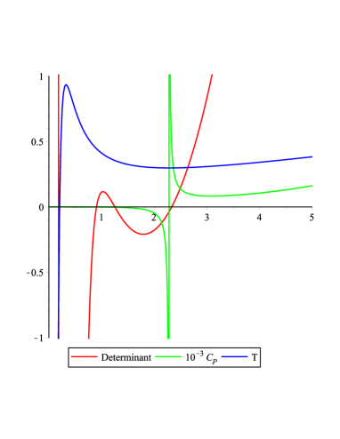
Figure 2: Thermal stability in two ensembles with positive temperature for $e=0.5$, $\mathtt{C}_{i}=1$ and $P=\frac{1}{8\pi}$.

As we mentioned before, the mass term in (10) satisfies the first law of thermodynamics which in the extended phase space can be written as

$$dM=TdS+VdP+\sum_{i=1}^{3}\mathcal{C}_{i}d\mathtt{C}_{i}+\mathtt{e}\;de,$$ (21)

where the thermodynamic volume per $\Omega_{3}$ is defined as

$$V=\dfrac{\partial M}{\partial P}\bigg{|}_{r_{+},c_{i},e}=\dfrac{r_{+}^{4}}{4},$$ (22)

and conjugates to the massive parameters and the Yang-Mills coupling constant per unit volume $\Omega_{3}$ are, respectively,

$$\mathcal{C}_{i}=\dfrac{\partial M}{\partial c_{i}}\bigg{|}_{r_{+},P,e}=\dfrac{i(i+1)}{32\pi}r_{+}^{4-i},$$ (23)

and

$$\mathtt{e}=\dfrac{\partial M}{\partial e}\bigg{|}_{r_{+},P,c_{i}}=-\dfrac{3e}{4\pi}\ln(\frac{r_{+}}{L}).$$ (24)

Due to the existence of logarithmic term in the metric function, obtaining the Smarr formula is not a trivial task. To explore the Smarr formula, we need to define a new Yang-Mills variable

$$E^{2}=e^{2}\ln(\frac{r_{+}}{L}).$$ (25)

By substitution of this definition in the mass (10), one obtains the mass term per unit volume $\Omega_{3}$ as

$$M=\frac{3}{16\pi}\left(\frac{r_{+}^{4}}{\ell^{2}}+\frac{\mathtt{C}_{1}}{3}r_{+}^{3}+\mathtt{C}_{2}r_{+}^{2}+2\mathtt{C}_{3}r_{+}-2E^{2}\right),$$ (26)

where the temperature can be calculated as

$$T=\frac{1}{2\pi r_{+}^{3}}\left(\frac{2r_{+}^{4}}{\ell^{2}}+\frac{1}{2}\mathtt{C}_{1}r_{+}^{3}+\mathtt{C}_{2}r_{+}^{2}+\mathtt{C}_{3}r_{+}\right).$$ (27)

We should note that there is not any effect of Yang-Mills term in temperature (the last term in Eq. (II) eliminates). It is notable that although it seems $E$ depends on $r_{+}$, such a temperature that can be calculated from both the surface gravity and the first law may confirm that we should interpret $E$ as an independent thermodynamic quantity. In other words, one may adjust “$L$” such a way that the quantity $(\frac{r_{+}}{L})$ is considered as a constant. By doing dimensional analysis (for example with the help of Eq. (26)), the Smarr formula has been verified

$$2M=3TS-2VP-\mathcal{C}_{1}\mathtt{C}_{1}+\mathcal{C}_{3}\mathtt{C}_{3}+\mathcal{E}E,$$ (28)

where now we have $\mathcal{E}=\dfrac{\partial M}{\partial E}\bigg{|}_{r_{+},P,c_{i}}=-\dfrac{3E}{4\pi}$. Please note that the massive parameter $\mathtt{C}_{2}$ does not appear in the Smarr formula since it has no scaling and so it is not a thermodynamic variable. Moreover, for this reason, we can omit this parameter from the first law (21). The role of the new quantity $``E"$ in the Smarr formula suggests that one may consider $``E"$ as a thermodynamic variable instead of $``e"$ with the following explicit form

$$dM=TdS+VdP+\mathcal{C}_{1}d\mathtt{C}_{1}+\mathcal{C}_{3}d\mathtt{C}_{3}+\mathcal{E}dE.$$ (29)

IV PHOTON SPHERE AND SHADOW

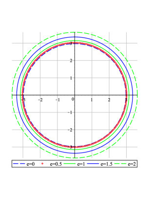
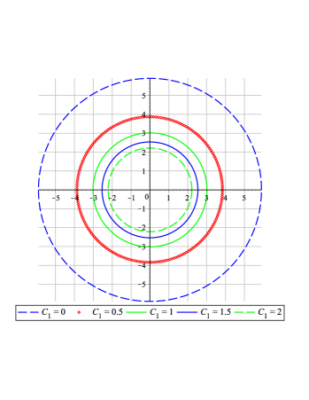
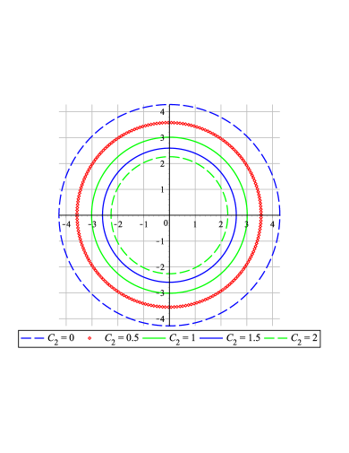
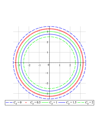
Figure 3: Black hole shadow in the Celestial plane ($\alpha-\beta$) for varying $e$ with $\mathtt{C}_{i}=1$ (up-left panel), varying $\mathtt{C}_{1}$ with $\mathtt{C}_{2}=\mathtt{C}_{3}=1$ and $e=0.5$ (up-right panel), varying $\mathtt{C}_{2}$ with $\mathtt{C}_{1}=\mathtt{C}_{3}=1$ and $e=0.5$ (down-left panel) and varying $\mathtt{C}_{3}$ with $\mathtt{C}_{1}=\mathtt{C}_{2}=1$ and $e=0.5$ (down-right panel). We set $M=L=\ell=1$.

It is quite clear that the strong gravitational field of black holes enforces propagation of light along curved lines such that the spherical light paths may arise (for example see Panpanich:2019mll ). If these photon orbits being unstable, then photons can scape to infinity and project on the Celestial sphere by a distant observer. Here, we study this phenomenon for the black hole solutions under consideration. The unstable critical photon orbit is known as the “photon sphere” and one may look for its radius depending on various parameters.

Considering the metric, Eqs. (4) and (5), we find that the coefficients are independent of $``t"$ and $``x_{i}"$. So, these symmetries imply the constants of motion $``-E"$ and $``L_{i}"$ for the time and $x_{i}~{}(i=1,2,3)$ directions, respectively. Now, we assume a test particle with rest mass $``m_{0}"$ moving around the black hole on a curve with an affine parameter $\lambda$. First, we should find the geodesic equations of motion using the Lagrangian

$$\mathcal{L}=\frac{1}{2}g_{\mu\nu}\dot{x}^{\mu}\dot{x}^{\nu};~{}~{}~{}\dot{x}^{\mu}=\frac{dx^{\mu}}{d\lambda}.$$ (30)

Substituting the metric from Eq. (4), we find

$$\mathcal{L}=-\frac{f(r)}{2}\left(\frac{dt}{d\lambda}\right)^{2}+\frac{1}{2f(r)}\left(\frac{dr}{d\lambda}\right)^{2}+\frac{r^{2}}{2b^{2}}\delta_{ij}\frac{dx^{i}}{d\lambda}\frac{dx^{j}}{d\lambda}.$$ (31)

Now, reminding the relations $E=-\frac{\partial\mathcal{L}}{\partial\dot{t}}$ and $L^{i}=\frac{\partial\mathcal{L}}{\partial\dot{x_{i}}}$, we can obtain the geodesic equations of motion as

$$\frac{dt}{d\lambda}=\frac{E}{f(r)},~{}~{}~{}~{}\frac{dx^{i}}{d\lambda}=\frac{b^{2}}{r^{2}}L^{i}.$$ (32)

The equation of motion in the radial direction can be derived from the Hamilton-Jacobi equation

$$S=\frac{1}{2}m_{0}^{2}\lambda-Et+L_{1}x_{1}+L_{2}x_{2}+L_{3}x_{3}+S_{r}(r),$$ (33)

where $S_{r}(r)$ is a function of $r$. This equation allows us to find

$$f(r)(\frac{\partial S_{r}}{\partial r})^{2}=-m_{0}^{2}+\frac{E^{2}}{f(r)}-\frac{b^{2}}{r^{2}}L^{2},$$ (34)

in which $L^{2}=L_{1}^{2}+L_{2}^{2}+L_{3}^{2}$. With the help of $p_{r}=\frac{\partial\mathcal{L}}{\partial\dot{r}}=\frac{\partial S}{\partial r}$, the null geodesic equation with $m_{0}=0$ is obtained in the following form

$$\left(\frac{dr}{d\lambda}\right)^{2}+V_{eff}(r)=0,$$ (35)

$$V_{eff}(r)\equiv-E^{2}+\frac{b^{2}}{r^{2}}f(r)L^{2}.$$ (36)

To have the spherical geodesics, we apply two conditions

$$V_{eff}(r)\bigg{|}_{r=r_{p}}=0,~{}~{}~{}\dfrac{\partial V_{eff}(r)}{\partial r}\bigg{|}_{r=r_{p}}=0,$$

where $r_{p}$ is the radius of photon orbit. The first condition results to

$$\dfrac{r_{p}^{2}}{b^{2}f(r_{p})}=\dfrac{L^{2}}{E^{2}},$$ (37)

and the second condition gives

$$-2f(r_{p})+r_{p}f^{\prime}(r_{p})=0.$$ (38)

Substituting the metric function (5) in the recent relation, we find

$$-\dfrac{1}{3}\mathtt{C}_{1}r_{p}^{3}-2\mathtt{C}_{2}r_{p}^{2}-6\mathtt{C}_{3}r_{p}+\dfrac{64\pi}{3}M+8e^{2}\ln(\dfrac{r_{p}}{L})-2e^{2}=0.$$ (39)

In general, analytical solution of this equation for $r_{p}$ is not a trivial task. However, for some special cases, one can find an analytical relation for the radius of photon sphere, as follow

• $e=0$

  $$r_{p}=\dfrac{\eta^{2}-2\eta\mathtt{C}_{2}-6\mathtt{C}_{1}\mathtt{C}_{3}+4\mathtt{C}_{2}^{2}}{\mathtt{C}_{1}\eta},$$ (40)

  where

  $$\eta = (32M\pi\mathtt{C}_{1}^{2}+18\mathtt{C}_{1}\mathtt{C}_{2}\mathtt{C}_{3}-8\mathtt{C}_{2}^{3}\pm 2\gamma^{\frac{1}{2}}\mathtt{C}_{1})^{\frac{1}{3}},$$

  $$\gamma = 32\pi M(8\pi M\mathtt{C}_{1}^{2}+9\mathtt{C}_{1}\mathtt{C}_{2}\mathtt{C}_{3}-4\mathtt{C}_{2}^{3})+$$

  $$27\mathtt{C}_{3}^{2}(2\mathtt{C}_{1}\mathtt{C}_{3}-\mathtt{C}_{2}^{2}).$$

• $\mathtt{C}_{i}$’s$=0$

  $$r_{p}=L~{}\exp\left(\frac{1}{4}-\frac{8\pi M}{3e^{2}}\right).$$ (41)

• If one of the $\mathtt{C}_{i}$’s is non zero, then $r_{p}$ is found in terms of the Lambert W function.

$\mathtt{C}_{1}$	$0$	$0.5$	$1$	$1.5$	$2$
$r_{p}(e=0.5$, $\mathtt{C}_{2}=\mathtt{C}_{3}=1$)	$4.58$	$4.09$	$3.78$	$3.55$	$3.38$
$\mathtt{C}_{2}$	$0$	$0.5$	$1$	$1.5$	$2$
$r_{p}(e=0.5$, $\mathtt{C}_{1}=\mathtt{C}_{3}=1)$	$4.94$	$4.26$	$3.78$	$3.42$	$3.14$
$\mathtt{C}_{3}$	$0$	$0.5$	$1$	$1.5$	$2$
$r_{p}(e=0.5$, $\mathtt{C}_{1}=\mathtt{C}_{2}=1)$	$4.46$	$4.11$	$3.78$	$3.46$	$3.17$
$e$	$0$	$0.5$	$1$	$1.5$	$2$
$r_{p}(\mathtt{C}_{1}=\mathtt{C}_{2}=\mathtt{C}_{3}=1)$	$3.72$	$3.78$	$3.97$	$4.29$	$4.74$

Table 3: Photon sphere radius for variation of massive and Yang-Mills parameters for $M=1$ and $L=1$.

It is possible to numerically show that there are two positive roots for the Eq. (39), which are larger than the event horizon radius and therefore we have two small and large spherical light orbits. To know which one is stable with respect to the radial perturbations, we rely on the sign of the second derivative of $V_{eff}(r)$, where $V_{eff}^{\prime\prime}(r_{p})>0$ indicates stable orbits and $V_{eff}^{\prime\prime}(r_{p})<0$ stands for unstable ones. The radius of the unstable photon sphere (the larger photon orbit) for some parameters is listed in table 3, thereby we understand the behavior of $r_{p}$ under variation of the massive and Yang-Mills parameters. We see that the radius decreases with increasing the massive parameters while keeping the Yang-Mills parameter constant. Furthermore, with constant massive parameters, we observe that the bigger Yang-Mills parameter is, the larger photon sphere we have.

To discuss the black hole shadow, we consider one luminous source behind the black hole with a strong gravitational field to lens the radiation coming from the source. We change the Cartesian coordinates of the horizon to the spherical ones to have more straightforward calculations. One can follow the calculations of Ref. Das:2019sty for the shadow radius of black holes with spherically symmetric metric. For this purpose, we go to the Celestial coordinates which are introduced with $\alpha$ as the perpendicular distance of the shadow from the axis of symmetry and $\beta$ as the apparent perpendicular distance of the shadow from its projection on the equatorial plane. In this way, we get an equation representing a circle of radius $R_{s}$ in the Celestial plane $\alpha-\beta$, given by

$$\alpha^{2}+\beta^{2}=R_{s}^{2}=\dfrac{\dfrac{r_{p}^{2}}{f(r_{p})}}{1-\dfrac{r_{p}^{2}}{f(r_{p})}\dfrac{f(r_{o})}{r_{o}^{2}}},$$ (42)

where subscripts $``p"$ and $``o"$ denote the photon sphere and observer, respectively. Considering Eq. (5), one finds $\frac{f(r_{o})}{r_{o}^{2}}\rightarrow\frac{1}{\ell^{2}}$ (asymptotic AdS spacetime) for the limit $r_{o}\rightarrow\infty$ for the distant observer. So the radius of shadow calculating by a distant observer is given by

$$R_{s}=\frac{\ell}{\sqrt{\frac{f(r_{p})\ell^{2}}{r_{p}^{2}}-1}},$$ (43)

in which for the asymptotically flat black hole, it reduces to $R_{s}=\frac{r_{p}}{\sqrt{f(r_{p})}}$.

In Fig. 3, we plot the black hole shadow for different Yang-Mills and massive parameters. We find that the shadow size shrinks with decreasing $``e"$ (increasing $\mathtt{C}_{i}$), which is analogous with the obtained results for the variation of photon sphere radius. Furthermore, we see that variation of $``e"$ has weaker effect on the shadow size than the massive parameters, while more significant effect is occurred for $\mathtt{C}_{1}$.

V Quasinormal Modes

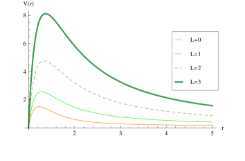
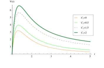
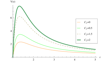
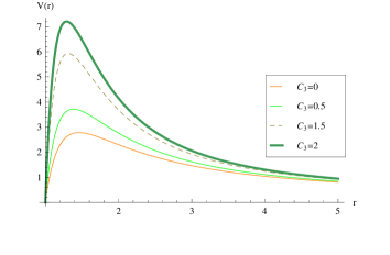
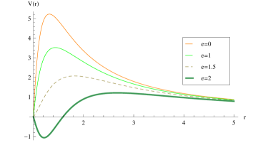
Figure 4: Effective potential for $\mathtt{C}_{1}=\mathtt{C}_{2}=\mathtt{C}_{3}=1$, $e$=0.5 with different $L$ (up-left panel), $\mathtt{C}_{2}=\mathtt{C}_{3}=1$, $e=0.5$ with $L=2$ (up-right panel), $\mathtt{C}_{1}=\mathtt{C}_{3}=1$, $e=0.5$ with $L=2$ (middle-left panel), $\mathtt{C}_{1}=\mathtt{C}_{2}=1$, $e=0.5$ with $L=2$ (middle-right panel), $\mathtt{C}_{1}=\mathtt{C}_{2}=\mathtt{C}_{3}=1$ with $L=2$ (down panel).

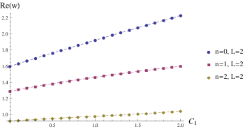
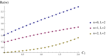
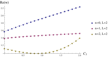
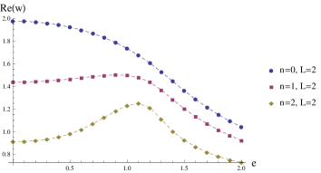
Figure 5: Real part of scalar quasinormal modes for $\mathtt{C}_{2}=\mathtt{C}_{3}=1$, $e$=0.5 (up-left panel), $\mathtt{C}_{1}=\mathtt{C}_{3}=1$, $e$=0.5 (up-right panel), $\mathtt{C}_{1}=\mathtt{C}_{2}=1$, $e$=0.5 (down-left panel), $\mathtt{C}_{1}=\mathtt{C}_{2}=\mathtt{C}_{3}=1$ (down-right panel).

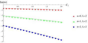
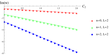
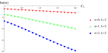
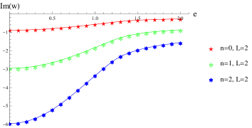
Figure 6: Imaginary part of scalar quasinormal modes with the same panel-coding as in Fig. 5

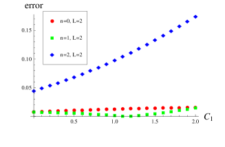
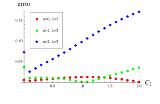
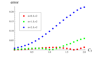
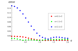
Figure 7: Error estimation of scalar quasinormal modes with the same panel-coding as in Fig. 5

In this section, we consider scalar perturbations around the black hole to find the quasinormal mode frequencies. In this regard, we use the WKB method which was first introduced by Schutz and Will to the third order Schutz:1985km and then extended to the 6th order Konoplya:2003ii and recently to the 13th order Konoplya:2019hlu .

The equation of motion for a scalar field is given by $\nabla^{\mu}\nabla_{\mu}\Phi=0$. Using separation of variables, the scalar field can be written as $\Phi(x^{\mu})=\sum\frac{\Psi_{L}(r)}{r}Y_{Lm}(\theta,\phi)e^{-i\omega t}$ where $L$ denotes multipole quantum number and $\omega$ is generally a complex number with the real part as the frequency and imaginary part as the decaying rate of QNMs. Regarding the spherical symmetry of the metric, with the help of spherical harmonics, one can write $\Delta Y(\theta,\varphi)=-L(L+1)Y(\theta,\varphi)$. Introducing the tortoise coordinate $r_{*}=\int\frac{dr}{f(r)},$ it is possible to write the radial part of the wave equation as follows

$$\frac{d^{2}\Psi}{dr_{*}^{2}}+[\omega^{2}-V(r)]\Psi(r_{*})=0,$$ (44)

where the effective potential is given as

$$V(r)=f(r)\Big{(}\frac{f^{\prime}(r)}{r}+\frac{L(L+1)}{r^{2}}\Big{)}.$$ (45)

The WKB method is used for effective potentials with the form of a potential barrier and constant values at the event horizon and spatial infinity. Thus, we consider asymptotically flat metric to have constant behavior at spatial infinity. The effective potential for some values of parameters is plotted in Fig. 4. We see that the conditions are satisfied except for the case of $e=2$ in the last panel with a potential pit before the barrier. Although it may pose inaccuracy, however, we also do calculation for this excepting case and we back this subtlety after the error estimations found.

It should be noted that increasing the WKB order does not always lead to a better approximation for the frequency, so we consider calculations at the 6th order approximation. As an example, the real and imaginary values of quasinormal modes for $L=2$ and $n=0,1,2$ are shown in Figs. 5 and 6, respectively. In both figures, each parameter is varied from $0-2$ at fixed other parameters. We observe that as the massive parameters $\mathtt{C}_{i}(i=1,2,3)$ increase, the real and imaginary (in magnitude) parts of the quasinormal frequencies grow mostly on a straight line. It means that higher energy modes decay faster. As an exception, the behavior of the real part for mode $L=2,n=2$ is not trivial as $\mathtt{C}_{3}$ increases and Re ($\omega$) is shrinking for variation of $\mathtt{C}_{3}$ from $0-1$. It seems that as the effect of massive gravitons gets stronger, the energy of the QNMs grows but, with a shorter lifetime, they decay faster.

However, for constant massive parameters, we observe that Re ($\omega$) and Im ($\omega$) (in magnitude) get lower with increasing the Yang-Mills parameter while the real part of mode $L=2,n=2$ has growing behavior for $e$ between $0$ and $1.1$. According to the figures, it seems that increasing “$e$” leads to appearing instability. In other words, one may find a critical value of “$e_{c}$” with respect to other parameters, in which the solutions are stable for $e<e_{c}$.

We find that as the overtone number $n$ increases, the scalar perturbations have less energy for oscillation and decay faster (with lower real and higher imaginary frequencies). From negative values for the imaginary frequency, we conclude that we have decaying oscillations, but as it is mentioned in Ref. Konoplya:2019hlu , it may not prove the stability of black hole because the method of WKB approximation always leads to $Im(\omega)<0$.

In order to estimate the error of the WKB approximation, one can compare two sequential orders. Here, we do this comparison between orders of six and seven such that the error approximation is defined by

$$\Delta\omega=\big{|}\dfrac{\omega_{7}-\omega_{6}}{\omega_{6}}\big{|}.$$ (46)

The error values are given in Fig. 7. We observe that the error estimation of $L=2$ and $n=2$ for $\mathtt{C}_{i}>1$ and $0<e<0.5$ becomes larger than 0.1 and then it seems that studying other known methods for obtaining quasinormal frequencies in this region could be helpful. Otherwise, the small values of error estimation guarantee enough accuracy for results. Moreover, from the last panel, we find the small error for $e=2$, though the potential, in this case, is not as the proper form.

VI Conclusion

In this paper, we considered the Einstein-Massive-Yang-Mills gravity in $5-$dimensions. We obtained the thermodynamic quantities for the planar AdS solution and showed that the first law of thermodynamics has been satisfied. By defining a pressure proportional to the cosmological constant, we performed the criticality analysis in the extended phase space thermodynamics. From the given equation of state, analytical relations for the critical quantities were computed. We found that there exists just one specific critical point for the given parameters which leads to critical behavior, physically. By studying the effects of Yang-Mills and massive parameters on the critical quantities, two tables were given which showed that increasing the Yang-Mills parameter $``e"$ leads to increasing $r_{c}$ and decreasing $\mathcal{T}_{c}$ and $P_{c}$. In addition, by increasing the massive parameters $\mathtt{C_{2}}$ and $\mathtt{C_{3}}$ the opposite behavior has been observed. Moreover, since the critical quantities are independent of $\mathtt{C}_{1}$, its variation does not affect the critical behavior of the solution.

We also studied the phase transition and its properties through some figures. According to the $P-r_{+}$ diagram, we found a first order van der Waals like phase transition for $\mathcal{T}<\mathcal{T}_{c}$. Furthermore, the existence of two divergence points in $C_{p}-r_{+}$ plot and also the swallow-tail behavior in the $G-T$ diagram are the characteristics of the first order phase transition. All of these remarks guided us to find the fact that the planar AdS black hole can exhibit the van der Waals like phase transition between the small and large black holes. As we showed such behavior comes from the massive term of the solutions, while it does not occur for the planar solutions of the Einstein-AdS and Einstein-Yang-Mills-AdS models.

We should note that in order to have the van der Waals phase transition in Einstein-AdS, the existence of electric charge is necessary, in addition to the spherical topology of the horizon (see Ref. Dolan ; Kubiznak-Mann ). Although there is no abelian charge in our solution, the existence of massive term in the Lagrangian is sufficient to guarantee the existence of van der Waals like phase transition.

We continued by investigating the photon sphere and the shadow observed by a distant observer. The results showed that the radius of the photon sphere decreases with increasing the massive parameters (decreasing the Yang-Mills parameter). We presented the black hole shadow for different Yang-Mills and massive parameters. It is observed that the shadow size shrinks with decreasing $``e"$ and increasing $\mathtt{C}_{i}$, which is the same as the results obtained for variation of the photon sphere radius.

Finally, we calculated the quasinormal modes of scalar perturbation for $L=2$ and $n=0,1,2$. We found that as the massive parameters $\mathtt{C}_{i}(i=1,2,3)$ increase, the real and imaginary (in magnitude) parts of the quasinormal frequencies grow mostly on a straight line. But the behavior of the real part for mode $L=2,n=2$ is not trivial as $\mathtt{C}_{3}$ increases and Re ($\omega$) is shrinking for variation of $\mathtt{C}_{3}$ from $0-1$. For constant massive parameters, we observed that Re ($\omega$) and Im ($\omega$) (in magnitude) get lower with increasing the Yang-Mills parameter while the real part of mode $L=2,n=2$ has growing behavior for $e$ between $0$ and $1.1$.

As future work, it is interesting to find other black string/brane solutions of the alternative theories of gravity with non-trivial horizon topologies and discuss the possibility of the criticality and phase transition. In addition, it will be useful to generalize the obtained solution to higher dimensions and study the effect of dimensionality.

- (1) K. Akiyama et al. [Event Horizon Telescope], Astrophys. J. 875, L1 (2019).
- (2) V. I. Dokuchaev and N. O. Nazarova, Phys. Usp., accepted (DOI: 10.3367/UFNe.2020.01.038717) [arXiv:1911.07695 [gr-qc]].
- (3) C. Bambi, K. Freese, S. Vagnozzi and L. Visinelli, Phys. Rev. D 100, 044057 (2019).
- (4) J. Moffat, Eur. Phys. J. C 75, 130 (2015).
- (5) B.P. Abbott et al. [LIGO Scientific and Virgo Collaborations], Phys. Rev. Lett. 116, 061102 (2016); Phys. Rev. Lett. 116, 221101 (2016); Phys. Rev. Lett. 116, 241103 (2016).
- (6) R. Konoplya and A. Zhidenko, Rev. Mod. Phys. 83, 793 (2011).
- (7) S. Ponglertsakul, P. Burikham and L. Tannukij, Eur. Phys. J. C 78, 584 (2018).
- (8) S. H. Hendi and M. Momennia, JHEP 10, 207 (2019).
- (9) F. Moulin, A. Barrau and K. Martineau, Universe 5, 202 (2019).
- (10) D. Zou, Y. Liu and R. Yue, Eur. Phys. J. C 77, 365 (2017).
- (11) P. Burikham, S. Ponglertsakul and L. Tannukij, Phys. Rev. D 96, 124001 (2017).
- (12) C. Chen, R. Nakarachinda and P. Wongjun, [arXiv:1910.05908 [gr-qc]].
- (13) P. Prasia and V. C. Kuriakose, Gen. Rel. Grav. 48, 89 (2016).
- (14) D. Kubiznak, R. B. Mann and M. Teo, Class. Quant. Grav. 34, 063001 (2017).
- (15) S. H. Hendi, R. B. Mann, S. Panahiyan and B. Eslam Panah, Phys. Rev. D 95, 021501 (2017).
- (16) C. de Rham and G. Gabadadze, Phys. Rev. D 82, 044020 (2010).
- (17) C. de Rham, G. Gabadadze and A. J. Tolley, Phys. Rev. Lett. 106, 231101 (2011).
- (18) C. de Rham, Living Rev. Rel. 17, 7 (2014).
- (19) R. G. Cai, Y. P. Hu, Q. Y. Pan and Y. L. Zhang, Phys. Rev. D 91, 024032 (2015).
- (20) S. H. Hendi, S. Panahiyan, B. Eslam Panah and M. Momennia, Annalen Phys. 528, 819 (2016).
- (21) S. G. Ghosh, L. Tannukij and P. Wongjun, Eur. Phys. J. C 76, 119 (2016).
- (22) S. H. Hendi, B. Eslam Panah and S. Panahiyan, Phys. Lett. B 769, 191 (2017).
- (23) D. C. Zou, R. Yue and M. Zhang, Eur. Phys. J. C 77, 256 (2017).
- (24) M. Zhang, Z. Y. Yang, D. C. Zou, W. Xu and R. H. Yue, Gen. Rel. Grav. 47, 14 (2015).
- (25) H. El Moumni, Phys. Lett. B 776, 124 (2018).
- (26) K. Meng, D. B. Yang and Z. N. Hu, Adv. High Energy Phys. 2017, 2038202 (2017).
- (27) A. Övgün, Adv. High Energy Phys. 2018, 8153721 (2018).
- (28) K. Meng and J. Li, Europhys. Lett. 116, 10005 (2016).
- (29) A. Dehghani and S. H. Hendi, Class. Quantum Grav. 37, 024001 (2020)
- (30) G. T. Horowitz, “Black holes in higher dimensions,” Cambridge University Press (2012).
- (31) P. S. Wesson, Int. J. Mod. Phys. D 24, 1530001 (2014).
- (32) M. Sadeghi, Eur. Phys. J. C 78, 875 (2018).
- (33) S. H. Hendi, S. Panahiyan and R. Mamasani, Gen. Relativ. Gravit. 47, 91 (2015).
- (34) S. Panpanich, S. Ponglertsakul and L. Tannukij, Phys. Rev. D 100, 044031 (2019).
- (35) A. Das, A. Saha and S. Gangopadhyay, Eur. Phys. J. C 80, 180 (2020).
- (36) B. F. Schutz and C. M. Will, Astrophys. J. 291, L33-L36 (1985).
- (37) R. Konoplya, Phys. Rev. D 68, 024018 (2003).
- (38) R. Konoplya, A. Zhidenko and A. Zinhailo, Class. Quant. Grav. 36, 155002 (2019).
- (39) B. P. Dolan, Class. Quant. Grav. 28, 125020 (2011).
- (40) D. Kubiznak and R. B. Mann, JHEP 07, 033 (2012).