SemEval-2013 Task 2: Sentiment Analysis in Twitter

Abstract

In recent years, sentiment analysis in social media has attracted a lot of research interest and has been used for a number of applications. Unfortunately, research has been hindered by the lack of suitable datasets, complicating the comparison between approaches. To address this issue, we have proposed SemEval-2013 Task 2: Sentiment Analysis in Twitter, which included two subtasks: A, an expression-level subtask, and B, a message-level subtask. We used crowdsourcing on Amazon Mechanical Turk to label a large Twitter training dataset along with additional test sets of Twitter and SMS messages for both subtasks. All datasets used in the evaluation are released to the research community. The task attracted significant interest and a total of 149 submissions from 44 teams. The best-performing team achieved an F1 of 88.9% and 69% for subtasks A and B, respectively.

1 Introduction

In the past decade, new forms of communication, such as microblogging and text messaging have emerged and become ubiquitous. Twitter messages (tweets) and cell phone messages (SMS) are often used to share opinions and sentiments about the surrounding world, and the availability of social content generated on sites such as Twitter creates new opportunities to automatically study public opinion.

Working with these informal text genres presents new challenges for natural language processing beyond those encountered when working with more traditional text genres such as newswire.

Tweets and SMS messages are short in length: a sentence or a headline rather than a document. The language they use is very informal, with creative spelling and punctuation, misspellings, slang, new words, URLs, and genre-specific terminology and abbreviations, e.g., RT for re-tweet and #hashtags. How to handle such challenges so as to automatically mine and understand the opinions and sentiments that people are communicating has only very recently been the subject of research [Jansen et al., 2009, Barbosa and Feng, 2010, Bifet et al., 2011, Davidov et al., 2010, O’Connor et al., 2010, Pak and Paroubek, 2010, Tumasjan et al., 2010, Kouloumpis et al., 2011].

Another aspect of social media data, such as Twitter messages, is that they include rich structured information about the individuals involved in the communication. For example, Twitter maintains information about who follows whom. Re-tweets (re-shares of a tweet) and tags inside of tweets provide discourse information. Modeling such structured information is important because it provides means for empirically studying social interactions where opinion is conveyed, e.g., we can study the properties of persuasive language or those associated with influential users.

Twitter	RT @tash_jade: That’s really sad, Charlie RT “Until tonight I never realised how fucked up I was” - Charlie Sheen #sheenroast
SMS	Glad to hear you are coping fine in uni… So, wat interview did you go to? How did it go?

Table 1: Examples of sentences from each corpus that contain subjective phrases.

Several corpora with detailed opinion and sentiment annotation have been made freely available, e.g., the MPQA corpus [Wiebe et al., 2005] of newswire text. These corpora have proved very valuable as resources for learning about the language of sentiment in general, but they did not focus on social media.

While some Twitter sentiment datasets have already been created, they were either small and proprietary, such as the i-sieve corpus [Kouloumpis et al., 2011], or they were created only for Spanish like the TASS corpus [Villena-Román et al., 2013], or they relied on noisy labels obtained from emoticons and hashtags. They further focused on message-level sentiment, and no Twitter or SMS corpus with expression-level sentiment annotations has been made available so far.

Thus, the primary goal of our SemEval-2013 task 2 has been to promote research that will lead to a better understanding of how sentiment is conveyed in Tweets and SMS messages. Toward that goal, we created the SemEval Tweet corpus, which contains Tweets (for both training and testing) and SMS messages (for testing only) with sentiment expressions annotated with contextual phrase-level polarity as well as an overall message-level polarity. We used this corpus as a testbed for the system evaluation at SemEval-2013 Task 2.

In the remainder of this paper, we first describe the task, the dataset creation process, and the evaluation methodology. We then summarize the characteristics of the approaches taken by the participating systems and we discuss their scores.

2 Task Description

We had two subtasks: an expression-level subtask and a message-level subtask. Participants could choose to participate in either or both subtasks. Below we provide short descriptions of the objectives of these two subtasks.

Subtask A: Contextual Polarity Disambiguation

Given a message containing a marked instance of a word or a phrase, determine whether that instance is positive, negative or neutral in that context. The boundaries for the marked instance were provided: this was a classification task, not an entity recognition task.

Subtask B: Message Polarity Classification

Given a message, decide whether it is of positive, negative, or neutral sentiment. For messages conveying both a positive and a negative sentiment, whichever is the stronger one was to be chosen.

Each participating team was allowed to submit results for two different systems per subtask: one constrained, and one unconstrained. A constrained system could only use the provided data for training, but it could also use other resources such as lexicons obtained elsewhere. An unconstrained system could use any additional data as part of the training process; this could be done in a supervised, semi-supervised, or unsupervised fashion.

Instructions: Subjective words are ones which convey an opinion. Given a sentence, identify whether it is objective, positive, negative, or neutral. Then, identify each subjective word or phrase in the context of the sentence and mark the position of its start and end in the text boxes below. The number above each word indicates its position. The word/phrase will be generated in the adjacent textbox so that you can confirm that you chose the correct range. Choose the polarity of the word or phrase by selecting one of the radio buttons: positive, negative, or neutral. If a sentence is not subjective please select the checkbox indicating that ”There are no subjective words/phrases”. Please read the examples and invalid responses before beginning if this is your first time answering this hit.

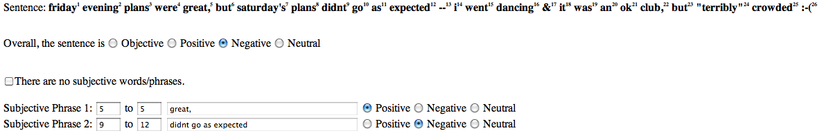
Figure 1: Instructions provided to workers on Mechanical Turk followed by a screenshot.

Note that constrained/unconstrained refers to the data used to train a classifier. For example, if other data (excluding the test data) was used to develop a sentiment lexicon, and the lexicon was used to generate features, the system would still be constrained. However, if other data (excluding the test data) was used to develop a sentiment lexicon, and this lexicon was used to automatically label additional Tweet/SMS messages and then used with the original data to train the classifier, then such a system would be unconstrained.

3 Dataset Creation

	Average # of		Total Phrase Count			Vocabulary
Corpus	Words	Characters	Positive	Negative	Neutral	Size
Twitter - Training	25.4	120.0	5,895	3,131	471	20,012
Twitter - Dev	25.5	120.0	648	430	57	4,426
Twitter - Test	25.4	121.2	2,734	1,541	160	11,736
SMS - Test	24.5	95.6	1,071	1,104	159	3,562

Table 2: Statistics for Subtask A.

In the following sections we describe the collection and annotation of the Twitter and SMS datasets.

3.1 Data Collection

Twitter is the most common micro-blogging site on the Web, and we used it to gather tweets that express sentiment about popular topics. We first extracted named entities using a Twitter-tuned NER system [Ritter et al., 2011] from millions of tweets, which we collected over a one-year period spanning from January 2012 to January 2013; we used the public streaming Twitter API to download tweets.

We then identified popular topics as those named entities that are frequently mentioned in association with a specific date [Ritter et al., 2012]. Given this set of automatically identified topics, we gathered tweets from the same time period which mentioned the named entities. The testing messages had different topics from training and spanned later periods.

To identify messages that express sentiment towards these topics, we filtered the tweets using SentiWordNet [Baccianella et al., 2010]. We removed messages that contained no sentiment-bearing words, keeping only those with at least one word with positive or negative sentiment score that is greater than 0.3 in SentiWordNet for at least one sense of the words. Without filtering, we found class imbalance to be too high.

Corpus	Positive	Negative	Objective
			/ Neutral
Twitter - Training	3,662	1,466	4,600
Twitter - Dev	575	340	739
Twitter - Test	1,573	601	1,640
SMS - Test	492	394	1,208

Table 3: Statistics for Subtask B.

Twitter messages are rich in social media features, including out-of-vocabulary (OOV) words, emoticons, and acronyms; see Table 1. A large portion of the OOV words are hashtags (e.g., #sheenroast) and mentions (e.g., @tash_jade).

We annotated the same Twitter messages with annotations for subtask A and subtask B. However, the final training and testing datasets overlap only partially between the two subtasks since we had to throw away messages with low inter-annotator agreement, and this differed between the subtasks. For testing, we also annotated SMS messages, taken from the NUS SMS corpus [Chen and Kan, 2012]. Tables 2 and  3 show statistics about the corpora we created for subtasks A and B.

3.2 Annotation Guidelines

The instructions provided to the annotators, along with an example, are shown in Figure 1. We provided several additional examples to the annotators, shown in Table 5.

	A			B
	Lower	Avg.	Upper	Avg.
Twitter - Train	64.7	82.4	90.8	82.7
Twitter - Dev	51.2	74.7	87.8	78.4
Twitter - Test	68.8	83.6	90.9	76.9
SMS - Test	66.5	88.5	81.2	77.6

Table 4: Bounds for datasets in subtasks A and B.

Authorities are only too aware that Kashgar is 4,000 kilometres (2,500 miles) from Beijing but only a tenth of the distance from the Pakistani border, and are desperate to ensure instability or militancy does not leak over the frontiers.
Taiwan-made products stood a good chance of becoming even more competitive thanks to wider access to overseas markets and lower costs for material imports, he said.
”March appears to be a more reasonable estimate while earlier admission cannot be entirely ruled out,” according to Chen, also Taiwan’s chief WTO negotiator.
friday evening plans were great, but saturday’s plans didnt go as expected – i went dancing & it was an ok club, but terribly crowded :-(
WHY THE HELL DO YOU GUYS ALL HAVE MRS. KENNEDY! SHES A FUCKING DOUCHE
AT&T was okay but whenever they do something nice in the name of customer service it seems like a favor, while T-Mobile makes that a normal everyday thin
obama should be impeached on TREASON charges. Our Nuclear arsenal was TOP Secret. Till HE told our enemies what we had. #Coward #Traitor
My graduation speech: ”I’d like to thanks Google, Wikipedia and my computer! :D #iThingteens

Table 5: List of example sentences with annotations that were provided to the annotators. All subjective phrases are italicized. Positive phrases are in green, negative phrases are in red, and neutral phrases are in blue.

In addition, we filtered spammers by considering the following kinds of annotations invalid:

• containing overlapping subjective phrases;

• subjective but without a subjective phrase;

• marking every single word as subjective;

• not having the overall sentiment marked.

3.3 Annotation Process

Our datasets were annotated for sentiment on Mechanical Turk. Each sentence was annotated by five Mechanical Turk workers (Turkers). In order to qualify for the hits, the Turker had to have an approval rate greater than 95% and have completed 50 approved hits. Each Turker was paid three cents per hit. The Turker had to mark all the subjective words/phrases in the sentence by indicating their start and end positions and say whether each subjective word/phrase was positive, negative, or neutral (subtask A). They also had to indicate the overall polarity of the sentence (subtask B).

Figure 1 shows the instructions and an example provided to the Turkers. The first five rows of Table 6 show an example of the subjective words/phrases marked by each of the workers.

For subtask A, we combined the annotations of each of the workers using intersection as indicated in the last row of Table 6. A word had to appear in 2/3 of the annotations in order to be considered subjective. Similarly, a word had to be labeled with a particular polarity (positive, negative, or neutral) 2/3 of the time in order to receive that label.

We also experimented with combining annotations by computing the union of the sentences, and taking the sentence of the worker who annotated the most hits, but we found that these methods were not as accurate. Table 4 shows the lower, average, and upper bounds for all the hits by computing the bounds for each hit and averaging them together. This gives a good indication about how well we can expect the systems to perform. For example, even if we used the best annotator each time, it would still not be possible to get perfect accuracy.

For subtask B, the polarity of the entire sentence was determined based on the majority of the labels. If there was a tie, the sentence was discarded. In order to reduce the number of sentences lost, we combined the objective and the neutral labels, which Turkers tended to mix up. Table 4 shows the average bound for subtask B by computing the bounds for each hit and averaging them together. Since the polarity is chosen based on the majority, the upper bound is 100%.

Worker 1	I would love to watch Vampire Diaries :) and some Heroes! Great combination	9/13
Worker 2	I would love to watch Vampire Diaries :) and some Heroes! Great combination	11/13
Worker 3	I would love to watch Vampire Diaries :) and some Heroes! Great combination	10/13
Worker 4	I would love to watch Vampire Diaries :) and some Heroes! Great combination	13/13
Worker 5	I would love to watch Vampire Diaries :) and some Heroes! Great combination	11/13
Intersection	I would love to watch Vampire Diaries :) and some Heroes! Great combination

Table 6: Example of a sentence annotated for subjectivity on Mechanical Turk. Words and phrases that were marked as subjective are italicized and highlighted in bold. The first five rows are annotations provided by Turkers, and the final row shows their intersection. The final column shows the accuracy for each annotation compared to the intersection.

4 Scoring

For both subtasks, the participating systems were required to perform a three-way classification – a particular marked phrase (for subtask A) or an entire message (for subtask B) was to be classified as positive, negative, or objective. For each system, we computed a score for predicting positive/negative phrases/messages vs. the other two classes.

For instance, to compute positive precision, $P_{pos}$, we find the number of phrases/messages that a system correctly predicted to be positive, and we divide that number by the total number of messages it predicted to be positive. To compute recall, for the positive class, $R_{pos}$, we find the number of messages correctly predicted to be positive and we divide that number by the total number of positive messages in the gold standard.

We then calculate F-score for the positive labels, the harmonic average of precision and recall as follows $F_{pos}=2\frac{P_{pos}R_{pos}}{P_{pos}+R_{pos}}$. We carry out a similar computation to calculate $F_{neg}$, which is F1 for negative messages.

The overall score for each system run is then given by the average of the F1-scores for the positive and negative classes: $F=(F_{pos}+F_{neg})/2$.

Note that ignoring $F_{neutral}$ does not reduce the task to predicting positive vs. negative labels only (even though some participants have chosen to do so) since the gold standard still contains neutral labels which are to be predicted: $F_{pos}$ and $F_{neg}$ would suffer if these examples are labeled as positive and/or negative instead of neutral.

We provided participants with a scorer. In addition to outputting the overall F-score, it produced a confusion matrix for the three prediction classes (positive, negative, and objective), and it also validated the data submission format.

Run	Const-	Unconst-	Use	Super-
	rained	rained	Neut.?	vised?
NRC-Canada	88.93		yes	yes
AVAYA	86.98	87.38(1)	yes	yes
BOUNCE	86.79		yes	yes
LVIC-LIMSI	85.70		yes	yes
FBM	85.50		yes	semi
GU-MLT-LT	85.19		yes	yes
⋄UNITOR	84.60		yes	yes
USNA	81.31		yes	yes
Serendio	80.04		yes	yes
⋄ECNUCS	79.48	80.15(2)	yes	yes
TJP	78.16		yes	yes
∘columbia-nlp	74.94		yes	yes
teragram		74.89(3)	yes	yes
sielers	74.41		yes	yes
KLUE	73.74		yes	yes
OPTWIMA	69.17	36.91(6)	yes	yes
swatcs	67.19	63.86(5)	no	yes
Kea	63.94		yes	yes
senti.ue-en	62.79	71.38(4)	yes	yes
uottawa	60.20		yes	yes
IITB	54.80		yes	yes
SenselyticTeam	53.88		yes	yes
SU-sentilab		34.73(7)	no	yes
Majority Baseline	38.10		N/A	N/A

Table 7: Results for subtask A on the Twitter dataset. The ^∘ marks a team that includes a task coorganizer, and the ^⋄ indicates a system submitted as constrained but which used additional Tweets or additional sentiment-annotated text to collect statistics that were then used as a feature.

Run	Const-	Unconst-	Use	Super-
	rained	rained	Neut.?	vised?
GU-MLT-LT	88.37		yes	yes
NRC-Canada	88.00		yes	yes
⋆AVAYA	83.94	85.79(1)	yes	yes
⋄UNITOR	82.49		yes	yes
TJP	81.23		yes	yes
LVIC-LIMSI	80.16		yes	yes
USNA	79.82		yes	yes
⋄ECNUCS	76.69	77.34(2)	yes	yes
sielers	73.48		yes	yes
FBM	72.95		no	semi
teragram	72.83	72.83(4)	yes	yes
KLUE	70.54		yes	yes
∘columbia-nlp	70.30		yes	yes
senti.ue-en	66.09	74.13(3)	yes	yes
swatcs	66.00	67.68(5)	no	yes
Kea	63.27		yes	yes
uottawa	55.89		yes	yes
SU-sentilab		55.38(6)	no	yes
SenselyticTeam	51.13		yes	yes
OPTWIMA	37.32	36.38(7)	yes	yes
Majority Baseline	31.50		N/A	N/A

Table 8: Results for subtask A on the SMS dataset. The ^⋆ indicates a late submission, the ^∘ marks a team that includes a task co-organizer, and the ^⋄ indicates a system submitted as constrained but which used additional Tweets or additional sentiment-annotated text to collect statistics that were then used as a feature.

5 Participants and Results

The results for subtask A are shown in Tables 7 and 8 for Twitter and for SMS messages, respectively; those for subtask B are shown in Table 9 for Twitter and in Table 10 for SMS messages. Systems are ranked by their scores for the constrained runs; the ranking based on scores for unconstrained runs is shown as a subindex.

For both subtasks, there were teams that only submitted results for the Twitter test set. Some teams submitted both a constrained and an unconstrained version (e.g., AVAYA and teragram). As one would expect, the results on the Twitter test set tended to be better than those on the SMS test set since the SMS data was out-of-domain with respect to the training (Twitter) data.

Moreover, the results for subtask A were significantly better than those for subtask B, which shows that it is a much easier task, probably because there is less ambiguity at the phrase-level.

Run	Const-	Unconst-	Use	Super-
	rained	rained	Neut.?	vised?
NRC-Canada	69.02		yes	yes
GU-MLT-LT	65.27		yes	yes
teragram	64.86	64.86(1)	yes	yes
BOUNCE	63.53		yes	yes
KLUE	63.06		yes	yes
AMI&ERIC	62.55	61.17(3)	yes	yes/semi
FBM	61.17		yes	yes
AVAYA	60.84	64.06(2)	yes	yes/semi
SAIL	60.14	61.03(4)	yes	yes
UT-DB	59.87		yes	yes
FBK-irst	59.76		yes	yes
nlp.cs.aueb.gr	58.91		yes	yes
⋄UNITOR	58.27	59.50(5)	yes	semi
LVIC-LIMSI	57.14		yes	yes
Umigon	56.96		yes	yes
NILC_USP	56.31		yes	yes
DataMining	55.52		yes	semi
⋄ECNUCS	55.05	58.42(6)	yes	yes
nlp.cs.aueb.gr	54.73		yes	yes
ASVUniOfLeipzig	54.56		yes	yes
SZTE-NLP	54.33	53.10(9)	yes	yes
CodeX	53.89		yes	yes
Oasis	53.84		yes	yes
NTNU	53.23	50.71(10)	yes	yes
UoM	51.81	45.07(15)	yes	yes
SSA-UO	50.17		yes	no
SenselyticTeam	50.10		yes	yes
UMCC_DLSI_(SA)	49.27	48.99(12)	yes	yes
bwbaugh	48.83	54.37(8)	yes	yes/semi
senti.ue-en	47.24	47.85(13)	yes	yes
SU-sentilab		45.75(14)	yes	yes
OPTWIMA	45.40	54.51(7)	yes	yes
REACTION	45.01		yes	yes
uottawa	42.51		yes	yes
IITB	39.80		yes	yes
IIRG	34.44		yes	yes
sinai	16.28	49.26(11)	yes	yes
Majority Baseline	29.19		N/A	N/A

Table 9: Results for subtask B on the Twitter dataset. The ^⋄ indicates a system submitted as constrained but which used additional Tweets or additional sentiment-annotated text to collect statistics that were then used as a feature.

Run	Const-	Unconst-	Use	Super-
	rained	rained	Neut.?	vised?
NRC-Canada	68.46		yes	yes
GU-MLT-LT	62.15		yes	yes
KLUE	62.03		yes	yes
AVAYA	60.00	59.47(1)	yes	yes/semi
teragram		59.10(2)	yes	yes
NTNU	57.97	54.55(6)	yes	yes
CodeX	56.70		yes	yes
FBK-irst	54.87		yes	yes
AMI&ERIC	53.63	52.62(7)	yes	yes/semi
⋄ECNUCS	53.21	54.77(5)	yes	yes
UT-DB	52.46		yes	yes
SAIL	51.84	51.98(8)	yes	yes
⋄UNITOR	51.22	48.88(10)	yes	semi
SZTE-NLP	51.08	55.46(3)	yes	yes
SenselyticTeam	51.07		yes	yes
NILC_USP	50.12		yes	yes
REACTION	50.11		yes	yes
SU-sentilab		49.57(9)	no	yes
nlp.cs.aueb.gr	49.41	55.28(4)	yes	yes
LVIC-LIMSI	49.17		yes	yes
FBM	47.40		yes	yes
ASVUniOfLeipzig	46.50		yes	yes
senti.ue-en	44.65	46.72(12)	yes	yes
SSA_UO	44.39		yes	no
UMCC_DLSI_(SA)	43.39	40.67(14)	yes	yes
UoM	42.22	35.22(15)	yes	yes
OPTWIMA	40.98	47.15(11)	yes	yes
uottawa	40.51		yes	yes
bwbaugh	39.73	43.43(13)	yes	yes/semi
IIRG	22.16		yes	yes
Majority Baseline	19.03		N/A	N/A

Table 10: Results for subtask B on the SMS dataset. The ^⋄ indicates a system submitted as constrained but which used additional Tweets or additional sentiment-annotated text to collect statistics that were then used as a feature.

5.1 Subtask A: Contextual Polarity

Table 7 shows that subtask A, Twitter, attracted 23 teams, who submitted 21 constrained and 7 unconstrained systems. Five teams submitted both a constrained and an unconstrained system, and two other teams submitted constrained systems that are on the boundary between being constrained and unconstrained.

One system was semi-supervised, and the rest were supervised. The supervised systems used classifiers such as SVM (8 systems), Naive Bayes (7 systems), and Maximum Entropy (3 systems). Other approaches used include an ensemble of classifiers, manual rules, and a linear classifier. Two of the systems chose not to predict neutral as a possible classification label.

The average F1-measure on the Twitter test set was 74.1% for constrained systems and 60.5% for unconstrained ones; this does not mean that using additional data does not help, it just shows that the best teams only participated with a constrained system. NRC-Canada had the best constrained system with an F1-measure of 88.9%, and AVAYA had the best unconstrained one with F1=87.4%.

Table 8 shows the results for the SMS test set, where 20 teams submitted 19 constrained and 7 unconstrained systems (again, this included two teams that submitted boundary systems, marked accordingly). The average F-measure on this test set was 70.8% for constrained systems and 65.7% for unconstrained systems. The best constrained system was that of GU-MLT-LT with an F-measure of 88.4%, and AVAYA had the best unconstrained system with an F1 of 85.8%.

5.2 Subtask B: Message Polarity

Table 9 shows that subtask B, Twitter, attracted 38 teams, who submitted 36 constrained and 15 unconstrained systems (and two boundary ones).

The average F1-measure was 53.7% for the constrained and 54.6% for the unconstrained systems.

These averages are much lower than those for subtask A, which indicates that subtask B is harder, probably because a message can contain parts expressing both positive and negative sentiment.

Once again, NRC-Canada had the best constrained system with an F1-measure of 69%, followed by teragram, which had the best unconstrained system with an F1-measure of 64.9%.

As Table 10 shows, the average F1-measure on the SMS test set was 50.2% for constrained and 50.3% for unconstrained systems. NRC-Canada had the best constrained system with an F1=68.5%, and AVAYA had the best unconstrained one with F1-measure of 59.5%.

5.3 Overall

Overall, the results achieved by the best teams were very strong, especially for the simpler subtask A:

• F1=88.93, NRC-Canada on subtask A, Twitter;

• F1=88.37, GU-MLT-LT on subtask A, SMS;

• F1=69.02, NRC-Canada on subtask B, Twitter;

• F1=68.46, NRC-Canada on subtask B, SMS.

We can see that the strongest team overall was that of NRC-Canada, which was ranked first on three of the four conditions; and it was second on subtask A, SMS. There were two other teams that were strong across both tasks and on both test sets: GU-MLT-LT and AVAYA. Three other teams, namely teragram, BOUNCE and KLUE, were ranked in the top-3 in at least one subtask and test set.

6 Discussion

We have seen that most participants restricted themselves to the provided data and submitted constrained systems. Indeed, the best systems for each of the two subtasks and for each of the two testing datasets were constrained systems; of course, this does not mean that additional data would not be useful. Curiously, in some cases where a team submitted a constrained and unconstrained run, the unconstrained run actually performed worse.

Not surprisingly, most systems were supervised; there were only five semi-supervised systems, and there was only one unsupervised system. One additional team declared their system as unsupervised since it was not making use of the training data; we still classified it as supervised though since it did use supervision – in the form of manual rules.

Most participants predicted all three labels (positive, negative and neutral), even though some participants opted for not predicting neutral, which made some sense since the final F1-score was averaged over the positive and the negative predictions only.

The most popular classifiers included SVM, MaxEnt, linear classifier, Naive Bayes; in some cases, manual rules or ensembles of classifiers were used.

A variety of features were used, including word-related (e.g., words, stems, $n$-grams, word clusters), word-shape (e.g., punctuation, capitalization), syntactic (e.g., POS tags, dependency relations), Twitter-specific (e.g., repeated characters, emoticons, URLs, hashtags, slang, abbreviations), and sentiment-related (e.g., negation); one team also used discourse relations. Almost all participants relied heavily of various sentiment lexicons, the most popular ones being MPQA and SentiWordNet, as well as AFINN and Bing Liu’s Opinion Lexicon; some participants used their own lexicons – preexisting or built from the provided data.

Given that Twitter messages are noisy, most participants did some preprocessing, including tokenization, stemming, lemmatization, stopword removal, normalization/removal of URLs, hashtags, users, slang, emoticons, repeated vowels, punctuation; some even did pronoun resolution.

7 Conclusion

We have described a new task that entered SemEval-2013: task 2 on Sentiment Analysis on Twitter. The task has attracted a very high number of participants: 149 submissions from 44 teams.

We believe that the datasets that we have created as part of the task and which we have released to the community under a Creative Commons Attribution 3.0 Unported License, will be found useful by researchers beyond SemEval.

References

- [Baccianella et al., 2010] Stefano Baccianella, Andrea Esuli, and Fabrizio Sebastiani. 2010. SentiWordNet 3.0: An enhanced lexical resource for sentiment analysis and opinion mining. In Nicoletta Calzolari (chair), Khalid Choukri, Bente Maegaard, Joseph Mariani, Jan Odijk, Stelios Piperidis, Mike Rosner, and Daniel Tapias, editors, Proceedings of the Seventh International Conference on Language Resources and Evaluation, LREC ’10, pages 2200–2204, Valletta, Malta.
- [Barbosa and Feng, 2010] Luciano Barbosa and Junlan Feng. 2010. Robust sentiment detection on Twitter from biased and noisy data. In Proceedings of the 23rd International Conference on Computational Linguistics: Posters, COLING ’10, pages 36–44, Beijing, China.
- [Bifet et al., 2011] Albert Bifet, Geoffrey Holmes, Bernhard Pfahringer, and Ricard Gavaldà. 2011. Detecting sentiment change in Twitter streaming data. Journal of Machine Learning Research - Proceedings Track, 17:5–11.
- [Chen and Kan, 2012] Tao Chen and Min-Yen Kan. 2012. Creating a live, public short message service corpus: the NUS SMS corpus. Language Resources and Evaluation, pages 1–37.
- [Davidov et al., 2010] Dmitry Davidov, Oren Tsur, and Ari Rappoport. 2010. Semi-supervised recognition of sarcastic sentences in Twitter and Amazon. In Proceedings of the Fourteenth Conference on Computational Natural Language Learning, CoNLL ’10, pages 107–116, Uppsala, Sweden.
- [Jansen et al., 2009] Bernard J. Jansen, Mimi Zhang, Kate Sobel, and Abdur Chowdury. 2009. Twitter power: Tweets as electronic word of mouth. J. Am. Soc. Inf. Sci. Technol., 60(11):2169–2188.
- [Kouloumpis et al., 2011] Efthymios Kouloumpis, Theresa Wilson, and Johanna Moore. 2011. Twitter sentiment analysis: The Good the Bad and the OMG! In Lada A. Adamic, Ricardo A. Baeza-Yates, and Scott Counts, editors, Proceedings of the Fifth International Conference on Weblogs and Social Media, ICWSM’ 11, pages 538–541, Barcelona, Spain.
- [O’Connor et al., 2010] Brendan O’Connor, Ramnath Balasubramanyan, Bryan R. Routledge, and Noah A. Smith. 2010. From tweets to polls: Linking text sentiment to public opinion time series. In William W. Cohen and Samuel Gosling, editors, Proceedings of the Fourth International Conference on Weblogs and Social Media, ICWSM ’10, Washington, DC, USA.
- [Pak and Paroubek, 2010] Alexander Pak and Patrick Paroubek. 2010. Twitter based system: Using Twitter for disambiguating sentiment ambiguous adjectives. In Proceedings of the 5th International Workshop on Semantic Evaluation, SemEval ’10, pages 436–439, Los Angeles, CA, USA.
- [Ritter et al., 2011] Alan Ritter, Sam Clark, Mausam, and Oren Etzioni. 2011. Named entity recognition in tweets: an experimental study. In Proceedings of the Conference on Empirical Methods in Natural Language Processing, EMNLP ’11, pages 1524–1534, Edinburgh, United Kingdom.
- [Ritter et al., 2012] Alan Ritter, Mausam, Oren Etzioni, and Sam Clark. 2012. Open domain event extraction from twitter. In Proceedings of the 18th ACM SIGKDD international conference on Knowledge discovery and data mining, KDD ’12, pages 1104–1112, Beijing, China.
- [Tumasjan et al., 2010] Andranik Tumasjan, Timm O. Sprenger, Philipp G. Sandner, and Isabell M. Welpe. 2010. Predicting elections with Twitter: What 140 characters reveal about political sentiment. In William W. Cohen and Samuel Gosling, editors, Proceedings of the Fourth International Conference on Weblogs and Social Media, ICWSM ’10, pages 178–185, Washington, DC, USA. The AAAI Press.
- [Villena-Román et al., 2013] Julio Villena-Román, Sara Lana-Serrano, Eugenio Martínez-Cámara, and José Carlos González Cristóbal. 2013. TASS - Workshop on Sentiment Analysis at SEPLN. Procesamiento del Lenguaje Natural, 50:37–44.
- [Wiebe et al., 2005] Janyce Wiebe, Theresa Wilson, and Claire Cardie. 2005. Annotating expressions of opinions and emotions in language. Language Resources and Evaluation, 39(2-3):165–210.