Exact Solutions and Constraints on the Dark Energy Model in FRW Universe

Abstract

The inflationary epoch and the late time acceleration of the expansion rate of universe can be explained by assuming a gravitationally coupled scalar field. In this article, we propose a new method of finding exact solutions in the background of flat Friedmann-Robertson-Walker (FRW) cosmological models by considering both scalar field and matter where the scalar field potential is a function of the scale factor. Our method provides analytical expressions for equation of state parameter of scalar field, deceleration parameter and Hubble parameter. This method can be applied to various other forms of scalar field potential, to the early radiation dominated epoch and very early scalar field dominated inflationary dynamics. Since the method produces exact analytical expression for $H(a)$ (i.e., H(z) as well), we then constrain the model with currents data sets, which includes-Baryon Acoustic Oscillations, Hubble parameter data and Type 1a Supernova data (Pantheon Dataset). As an extension of the method, we also consider the inverse problem of reconstructing scalar field potential energy by assuming any general analytical expression of scalar field equation of state parameter as a function of scale factor.

rajib@iiserb.ac.in

#### #### #### ####

1 Introduction

The observations of type I-A supernovae indicate that expansion rate of the universe in the recent past (on cosmological time scale) is speeding up (Riess et al., 1998, Perlmutter et al., 1999, Tegmark et al., 2004, Spergel et al., 2007, Davis et al., 2007, Kowalski et al., 2008, Hicken et al., 2009, Komatsu et al., 2009, Hinshaw et al., 2009, Lima & Alcaniz, 2000, Lima et al., 2009, Basilakos & Plionis, 2010, Komatsu et al., 2011, Planck Collaboration et al., 2014, 2020). This discovery serves as a paradigm shift in our understanding of cosmology by postulating the existence of a component named ‘dark energy’. The analysis of current cosmological observations (Planck Collaboration et al., 2020) indicates that the ‘dark energy’ provides dominant contribution to the present total energy density of the universe. The accelerated expansion took place also in a widely separated time epoch, before the Universe became radiation dominated, during inflation (Guth, 1981), the theory of which was subsequently developed by  (Linde, 1982, 1983, Guth, 1981). The inflationary epoch as well as the recent accelerated expansion can be model led by postulating existence of a scalar field dynamically coupled to gravitation. Since a scalar field is a simple, yet natural candidate which causes accelerated expansion it plays a fundamental role in cosmology. Scalar fields have been extensively studied in cosmology (see (Ratra & Peebles, 1988, Linde, 1982, 1983, Peebles & Ratra, 2003, Bamba et al., 2012) and references therein). The scalar field, in this context, serves as the model of dark-energy. For the purpose of constraining the nature of dark-energy understanding the evolution of the universe during the accelerated expansion epoch of universe is an area of great research interest.

Currently, there is no unique underlying principle can uniquely specify the potential of the scalar field that gives rise to earlier inflationary epoch and the late time accelerated epoch of the universe. Many proposals based on new particle physics and gravitational theories were introduced (see (Linde, 2005) and references therein) and others were based on ad-hoc assumption so as to get the desired evolution of the universe (Ellis & Madsen, 1991). There is also a formalism where we can reconstruct the potential by using the knowledge of tensor gravitational spectrum and the scalar density fluctuation spectrum (Copeland et al., 1993, Liddle & Turner, 1994). Though there are numerous scalar field potential which can give rise to accelerated expansion, the exact solutions of these cosmological models are less known. As the exact solutions of cosmological models gives rise to exact cosmological parameters, they have a vital role in the present cosmological scenario. There are several methods by which one can explore the exact solutions of Friedman equations in a scalar field dominated universe. The construction of exact solutions for an inflationary scenario was started with Muslimov (Muslimov, 1990). The author, by starting with the assumption of scalar field potential $V(\phi)$, found the remaining parameters, i.e $a(t)$ and $\phi(t)$ based upon the model. A method of generating exact solutions in scalar field dominated cosmology by considering scalar field potential as a function of time $V(t)$ has been explored in (Zhuravlev et al., 1998). By assigning the time dependence of scale factor $a(t)$, we can also find the scalar field $\phi(t)$ and potential $V(t)$ as seen in (Ellis & Madsen, 1991). One can also find the analytical expressions for $a(t)$ and $V(\phi)$ by assigning time dependence of scalar field $\phi(t)$ which is explored in (Barrow, 1993). Barrow (Barrow, 1990) showed a simple method of finding exact solutions of cosmological dynamic equations in terms of a pressure-density relationship.

One can also reduce the scalar field cosmology equations to a known type of equation whose solution has already been developed. In (Harko et al., 2014, Chakrabarti, 2017) we can see a method in which the Klein-Gordon equation which describes the dynamics of the scalar field is transformed to a first order non-linear differential equation. This equation immediately leads to the identification of some exact classes of scalar field potentials $V(\phi)$ for which the field equations can be solved exactly and there by obtaining analytical expressions for $a(t)$, $\phi(t)$ and $q(t)$ . The solutions of the Friedman equations in a scalar field dominated universe is explored by its connection with the Abel equations of first kind is seen in (Yurov & Yurov, 2010). Here for a given $V(\phi)$ one can obtain $a(t)$ and $\phi(t)$ analytically. The exact solutions for exponential form of the potential $V(\phi)$ by rewriting the Klein-Gordon equation in the Riccati form and thereby transforming it into a second-order linear differential equation is investigated in (Andrianov et al., 2011). Analytical solutions to the field equations can also be obtained by considering suitable generating functions. Here the generating functions are chosen as a function of one of the parameters of the model (Kruger & Norbury, 2000, Charters & Mimoso, 2010, Harko et al., 2014, Chervon et al., 2018) and thus by simplifying the scalar field cosmology equation one can obtain all the parameters of the model. In (Salopek & Bond, 1990) a method was proposed by simplifying scalar field cosmology equation by assuming Hubble function as a function of scalar field $\phi$. By making use of the Noether symmetry for exponential potential (Paliathanasis et al., 2014, de Ritis et al., 1990), Hojman’s conservation law Capozziello & Roshan (2013), and other non-canonical conservation laws (Dimakis et al., 2016) for arbitrary potential and also by the form-invariant transformations of scalar field cosmology equations (Chimento et al., 2013) one can obtain the exact solutions for the parameters of the model. Moreover analytical solutions for field equations by considering a homogeneous scalar field in the Szekeres cosmological metric has been investigated in (Barrow & Paliathanasis, 2018).

Though there are various ways for finding exact solutions in scalar field cosmology, the solutions are limited if we incorporate the contributions by a perfect fluid source. In (Chimento & Jakubi, 1996) the authors showed that the Einstein’s equations with a self-interacting minimally coupled scalar field, a perfect fluid source and cosmological constant can be reduced to quadrature in the Robertson-Walker metric. Here the scale factor is considered as the independent variable and the scalar field potential is expressed in terms of scale factor. Barrow (Barrow & Saich, 1993) presented exact solutions of Friedman universes which contain a scalar field and a perfect fluid with the requirement that the kinetic and potential energies of the scalar field be proportional. The classes of scalar field potentials $V(\phi)$, which provide exact solutions for scalar field with scaling behavior had been investigated in (Liddle & Scherrer, 1999). In (Barrow & Paliathanasis, 2016) specific closed-form solutions of field equations(with and without matter source) have been derived by assuming special inflationary functions for the scale factor and special equation of state parameters of the scalar field. The application of lie symmetry methods in finding the exact cosmological solutions for scalar field dark energy in the presence of perfect fluids has been investigated in (Paliathanasis et al., 2015). In  (Socorro et al., 2015), a scenario of time varying cosmological term is investigated by using a special anartz were energy density of the scalar field is proportional to energy density of the barotropic fluid. Fomin (Fomin, 2018) explored the exact solutions by considering scalar field and matter fields or non-zero curvature by representing the main cosmological parameters as a function of number of $e$-folds and also by the direct substitution of the scale factor. The study of late-time cosmology in a (phantom) scalar-tensor theory with an exponential potential had been investigated in (Elizalde et al., 2004). In (Elizalde et al., 2008), the unification of inflation and late-time acceleration epochs within the context of a single field theory had been studied. Moreover, the exact and semiclassical solutions of the Wheeler-DeWitt equation for a particular family of scalar field potential had been explored in (Guzmán et al., 2007).

In this paper we propose a new method of finding analytical solutions of equation of state parameter of scalar field, deceleration parameter and also the Hubble parameter as a function of scale factor. Using the continuity equation for the scalar field we form a first order linear inhomogeneous equation of the independent variable $\dot{\phi}^{2}$ and dependent variable $a$. Since the inhomogeneous term is given by $-dV/da$, derivative of the scalar field $a$ the linear equation is exactly solvable for any choice of $V=V(a)$. As some test applications we present solutions for some chosen forms of $V(a)$. Since the linear equation is completely decoupled from the other source terms of the Friedmann equation the solution of $\dot{\phi}^{2}(a)$ and the chosen form of $V(a)$ can be used in the right hand side of first Friedmann equation together with the other source terms. Therefore, apart from the scalar field, our method can incorporate matter or radiation as a perfect fluid source to obtain an exact solution of $H(a)$ or $H(z)$, which can be constrained using observations. Since the method is applicable for any well behaved (e.g., differentiable w.r.t. $a$) chosen form of $V(a)$ it can be applied to understand the physics of the inflation, as well as the late time acceleration of expansion rate.

The paper is organized as follows. In Sec. 2 we explore the basis equations in scalar field cosmology. In Sec. 3.1 we consider the scalar field potential energy of power law form. The Sec. 4 is dedicated to the reconstruction of scalar field potential energy. After discussing the relationship of the scalar field potential with the particle physics models in Sec. 5, we constrain the model parameters in Sec. 6 Finally, in the last Sec. 7 we discuss and conclude upon our results.

2 Formalism

In the spatially flat Friedman-Robertson-Walker (FRW) model of the universe the space-time interval $ds$ between two events in a global comoving Cartesian coordinate system follows,

$$ds^{2}=dt^{2}-a^{2}(t)\bigl{(}dx^{2}+dy^{2}+dz^{2}\bigr{)}\,,$$ (1)

where $a$ and $t$ represent the scale factor and comoving time respectively and we have used $c=1$ unit. If the universe is dominated by the non-relativistic matter (e. g., baryon and cold dark matter) and a spatially homogeneous and time varying scalar field, $\phi$ which is minimally coupled to gravity, the evolution of $a(t)$ is determined by the following system of equations,

$$H^{2}\equiv\Big{(}\frac{\dot{a}}{a}\Big{)}^{2}=\frac{8\pi G}{3}\Big{[}\rho_{\phi}+\rho_{m}\Big{]}\,,$$ (2)

$$\frac{\ddot{a}}{a}=-\frac{4\pi G}{3}\Big{[}\rho_{m}+\rho_{\phi}+3(p_{m}+p_{\phi})\Big{]}\,,$$ (3)

where an over-dot represents derivative with respect to the comoving time $t$ and $\rho_{\phi}$ and $\rho_{m}$ represent the scalar field and matter density respectively. The time evolution of $\phi(t)$ couples to $a(t)$ and $V(\phi)$ and is governed by the second order generally non-linear differential equation,

$$\ddot{\phi}+3H\dot{\phi}+\frac{dV}{d\phi}=0\,.$$ (4)

We also have the continuity equation which holds separately for each component,

$$\dot{\rho}+3H\rho\bigl{(}1+\omega\bigr{)}=0\,,$$ (5)

where ${\omega}\equiv p/\rho$ represents the equation of state parameter for the component under consideration. The fluids filling the universe have equation of state given by,

$$p_{m}=0,\quad p_{\phi}=\omega_{\phi}\rho_{\phi}\,,$$ (6)

with

$$\rho_{m}=\frac{\rho^{0}_{m}}{a^{3}}~{},\quad\rho_{\phi}=\frac{\dot{\phi^{2}}}{2}+V,\quad p_{\phi}=\frac{\dot{\phi^{2}}}{2}-V\,.$$ (7)

Using $p_{\phi}$ and $\rho_{\phi}$ from Eqn. 7 in Eqn. 5 along with $p_{\phi}=\omega_{\phi}\rho_{\phi}$, we can rewrite continuity equation as follows,

$$\frac{d}{da}\Big{(}\frac{\dot{\phi^{2}}}{2}\Big{)}+\frac{dV}{da}+\frac{3}{a}\Big{(}\frac{\dot{\phi^{2}}}{2}\Big{)}=0\,.$$ (8)

Now, by considering $V=V(a)$ and using the transformation $\dot{\phi^{2}}(a)=y(a)$ we get the following linear differential equation,

$$\frac{dy}{da}+2\frac{dV}{da}+\frac{6}{a}y=0\,,$$ (9)

where we have assumed that $y$ and $V$ are in units of present day critical energy density $\rho^{0}_{c}$ such that,

$$y\rightarrow y^{\prime}=\frac{y}{\rho^{0}_{c}},\quad V\rightarrow V^{\prime}=\frac{V}{\rho^{0}_{c}}\,,$$ (10)

and omitted any primes in our forthcoming analysis of this work. The solution of linear differential equation 9 gives $\dot{\phi}^{2}(a)$ . Using Eqn. 10 the Friedmann Eqns. 2 and 3 become,

$$H^{2}(a)=H^{2}_{0}\left(\frac{\dot{\phi}^{2}}{2}+V(a)+\frac{\Omega^{0}_{m}}{a^{3}}\right)\,,$$ (11)

and

$$\frac{\ddot{a}}{a}=-H^{2}_{0}\left({\dot{\phi}^{2}}-V(a)+\frac{\Omega^{0}_{m}}{2a^{3}}\right)\,,$$ (12)

where we have assumed $p_{m}=0$. At this point, we mention that once a form of $V(a)$ is assumed, Eqn. 9 may be considered to be decoupled from the expansion dynamics of the universe, i.e., it does not depend on the exact solution of $a(t)$ which is obtained from first and second Friedman equations, Eqns. 11 and 12. This is an excellent advantage since the independent variable $y(a)$ can now be evolved irrespective of evolution of other components that contribute to the total energy momentum tensor. Another advantage of Eqn. 9 is that using its solution we immediately obtain the equation of state parameter of scalar field as, $\omega_{\phi}$ as

$$\omega_{\phi}(a)=\frac{{\dot{\phi^{2}}}/{2}-V}{{\dot{\phi^{2}}}/{2}+V}\,,$$ (13)

which serve as an important physical parameter to describe and constrain the nature of dark energy from both observational and theoretical point view. In this work, we focus ourselves for cases where both $\dot{\phi}^{2}$ and $V(a)$ are positive (semi) definite, resulting in $-1\leq\omega_{\phi}(a)\leq 1$.

Once $\dot{\phi}^{2}(a)$ is solved using Eqn. 9 for the assumed model of $V(a)$ one can relate the dynamics of the $\phi$ sector with some important dynamical variables of the dynamics of $a(t)$. One such variable is the total effective equation of state parameter, $\omega_{\textrm{t}ot}$ taking into account all components of the universe,

$$\omega_{\textrm{tot}}(a)\equiv\frac{p_{\phi}+p_{m}}{\rho_{\phi}+\rho_{m}}\equiv\frac{{\dot{\phi^{2}}(a)}/{2}-V(a)}{{\dot{\phi^{2}}(a)}{/2}+V(a)+{\Omega^{0}_{m}}/{a^{3}}}\,,$$ (14)

where $\Omega^{0}_{m}$ represents the present day energy density parameter for matter. The effective equation of state parameter, $\omega_{\textrm{tot}}$ has great significance because it tells us whether the universe undergoes an accelerated expansion ($\omega_{\textrm{tot}}<-1/3$) or decelerating expansion ($\omega_{\textrm{tot}}>-1/3$) at any particular epoch of time. Another useful parameter which encodes the information of acceleration or deceleration phases of $a(t)$ in its sign is the so-called deceleration parameter, $q$, defined as,

$$q=-\frac{\ddot{a}}{\dot{a^{2}}}a=-\frac{\ddot{a}}{a}\Big{(}\frac{\dot{a}}{a}\Big{)}^{-2}=-\frac{\ddot{a}}{a}\big{(}H\big{)}^{-2}\,.$$ (15)

A transition between the two phases always corresponds to zeros of the $q$ parameter. Since $\dot{\phi^{2}}(a)$, $V(a)$ and $\rho_{m}(a)$ are now known functions of scale factor, by using Eqn. 2 we can easily obtain the Hubble parameter, $H(a)$ . Knowing the numerator of Eqn. 15 using Eqn. 12 and denominator using Eqn. 11 we find an exact expression of $q(a)$ as well.

Before we proceed to discuss solution of Eqn. 9 for specific choice of $V(a)$ let us discuss some general features of these solutions. First, $a=0$ is a singular point of Eqn. 9. This means that the solution $\dot{\phi}^{2}(a)$ is not analytic at $a=0$. One common feature of $\dot{\phi}^{2}$ may be obtained by considering the associated homogeneous equation corresponding to Eqn. 9 by setting either $V=0$ or $V=V_{0}$, a constant for all $a$, so that $dV/da=0$. In this case, ignoring the trivial solution, $\dot{\phi}^{2}(a)=0$, we have $\dot{\phi}^{2}(a)=\dot{\phi}^{2}_{0}/a^{6}$. In fact, presence of a modulation factor of $\sim 1/a^{6}$ is ubiquitous in the solution of $\dot{\phi}^{2}(a)$ through the integrating factor of Eqn 9 for any other choice of $V(a)$. Thus $\dot{\phi}^{2}$ diverges in general, as $a\rightarrow 0$. This can be contrasted with the corresponding behavior for matter (or radiation) density, $\rho_{m}(a)=\rho^{0}_{m}/a^{3}$ ($\rho_{r}(a)=\rho^{0}_{r}/a^{4}$). We note that, such divergence of $\dot{\phi}^{2}(a)$ does not necessarily imply divergence of $\omega_{\phi}$, for a general $V(a)$. If $V=V_{0}$ we have $\omega_{\phi}(a)=\left(\dot{\phi}^{2}_{0}-2a^{6}V_{0}\right)/\left(\dot{\phi}^{2}_{0}+2a^{6}V_{0}\right)$, which tends to unity as $a\rightarrow 0$  .

3 Applications

3.1 Power Law Potential

Let us consider the power law form of potential energy density,

$$V(a)=V_{0}a^{n}\,,$$ (16)

where $V_{0}$ is a dimensionless constant and $n$ is a real number. By direct observation of Eqn. 9 we see that in this case, $\dot{\phi}^{2}(a)\sim a^{n}$ is a solution. If $n>1$ all terms of Eqn. 9 remains finite for all $a$. In fact, for any polynomial choice of

$$V(a)=\sum_{p=0}^{n}V_{p}a^{p+1}\,,$$ (17)

where $V_{p}$ for $p=1,....,n$ are constants, $\dot{\phi}^{2}(a)$ also admits a polynomial solution

$$\dot{\phi}^{2}(a)=\sum_{p=0}^{n}A_{p}a^{p+1}\,,$$ (18)

which is finite for all $a$. In this case, 9 becomes,

$$\sum_{p=0}^{n}A_{p}\left(p+7\right)a^{p}=-2\sum_{p=0}^{n}V_{p}(p+1)a^{p}\,,$$ (19)

which leads to a solution of the form

$$\dot{\phi}^{2}(a)=-2\sum_{p=0}^{n}\frac{V_{p}\left(p+1\right)}{\left(p+7\right)}a^{p+1}\,.$$ (20)

Eqn. 20 does not capture the complete picture of the most general solution $\dot{\phi}^{2}(a)$ since it only corresponds to the solution of the in-homogeneous Eqn. 9. The general solution of Eqn. 9 is obtained after adding with Eqn. 20 $C/a^{6}$, which is the solution corresponding to the homogeneous equation of Eqn. 9, where $C$ is a constant. The general solution is therefore,

$$\dot{\phi}^{2}(a)=-2\sum_{p=0}^{n}\frac{V_{p}\left(p+1\right)}{\left(p+7\right)}a^{p+1}+\frac{C}{a^{6}}\,.$$ (21)

The constant $C$ is fixed by imposing suitable boundary condition. If the potential energy density consists of a single power law as given by Eqn. 16, the only value of $p$ in Eqn. 21 becomes $p=n-1$. Eqn. 21 now becomes,

$$\dot{\phi^{2}}(a)\equiv y(a)=\frac{1}{a^{6}}\Big{(}-\frac{2V_{0}na^{n+6}}{n+6}+C\Big{)}\,,$$ (22)

where $n\neq-6$. If at $t=t_{0}$, $a=a_{0}=1$ and $\dot{\phi^{2}}(1)=y_{0}$, then $\rho^{0}_{\phi}+\rho^{0}_{m}=\rho^{0}_{c}=3H^{2}_{0}/(8\pi G)$, which following the definitions of Eqn. 10 implies,

$${y_{0}}=2\bigl{(}1-V_{0}-\Omega^{0}_{m}\bigr{)}\,.$$ (23)

Using Eqns. 22 and  23 we obtain,

$$C=y_{0}+\frac{2V_{0}n}{n+6}=2\biggl{[}\frac{n+6\left(1-V_{0}\right)}{n+6}\biggr{]}-2\Omega^{0}_{m}\,,$$ (24)

Finally using Eqns. 22 and 24 we obtain,

$$\dot{\phi^{2}}(a)=\frac{1}{a^{6}}\Bigg{[}2\biggl{(}\frac{n+6\left(1-V_{0}\right)}{n+6}\biggr{)}-\frac{2V_{0}na^{n+6}}{n+6}-2\Omega^{0}_{m}\Bigg{]}\,.$$ (25)

To get some insight into the nature of the solution given by Eqn. 25 we first consider a simple case for which $n=0$ (implying $V=V_{0}$, a constant) and $\Omega^{0}_{m}=0$ as well. This corresponds to a dark energy dominated flat universe with $\dot{\phi^{2}}_{0}=2(1-V_{0})$. If $V_{0}\neq 1$, $V\neq 1$ for always and using Eqn. 25,

$$\dot{\phi}^{2}(a)=\frac{2(1-V_{0})}{a^{6}}\,,$$ (26)

implying the kinetic energy density of the scalar field decays as $\sim a^{-6}$ as the universe expands. One can further consider two limiting values of $V_{0}$, namely, $1$ and $0$ respectively. If $V_{0}=1$ then from Eqn. 25 $\dot{\phi}^{2}(a)=0$ for all $a$ implying $\phi$ is a constant. In this case, as expected, we recover the cosmological model with cosmological constant with $\omega_{\phi}(a)=-1$. If $V_{0}=0$, $\dot{\phi}^{2}_{0}=2$ to satisfy the flatness condition today. In this case, $\omega_{\phi}=1$ always and hence the particular scalar field theory does not cause inflation. Using Eqn. 26 we obtain $\dot{\phi}^{2}(a)=2/a^{6}$. Substituting this in first Friedmann equation with $\Omega^{0}_{m}=0$ and after some algebra one finds,

$$a(t)=\big{(}H_{0}\big{)}^{1/3}t^{1/3}\,,$$ (27)

where we have used boundary condition $a=0$ at $t=0$. Clearly this particular scalar field does not cause inflation as argued earlier since $\omega_{\phi}=1$. In summary, we conclude that for different choices of numerical values of $V_{0}$ and specific choice of exponent $n$ in Eqn. 16 the solutions $\dot{\phi}^{2}(a)$ as given by Eqn. 9 are capable of capturing a wide range of dynamical behavior of scale factor $a(t)$.

Using the general solution $\dot{\phi}^{2}(a)$ (Eqn. 25) and Eqn. 16 in Eqn. 13 and Eqn. 14 respectively, we obtain,

$$\omega_{\phi}=\frac{n+6(1-V_{0})-\Omega^{0}_{m}(n+6)-2V_{0}(n+3)a^{n+6}}{n+6(1-V_{0})-\Omega^{0}_{m}(n+6)+6V_{0}a^{n+6}}\,,$$ (28)

and

$$\begin{split}\omega_{\textrm{tot}}=\Bigg{(}n+6(1-V_{0})-\Omega^{0}_{m}(n+6)-2V_{0}(n+3)a^{n+6}\Bigg{)}\Bigg{/}\\ \Bigg{(}n+6(1-V_{0})-\Omega^{0}_{m}(n+6)+6V_{0}a^{n+6}+\Omega^{0}_{m}a^{3}(n+6)\Bigg{)}\,.\end{split}$$ (29)

One can also easily calculate the Hubble parameter $H(a)$ as a function of scale factor using the Eqn. 11,

$$\begin{split}H^{2}(a)=H_{0}^{2}\Biggl{[}\frac{1}{a^{6}}\Biggl{(}\frac{n+6(1-V_{0})}{n+6}-\Omega^{0}_{m}-\frac{V_{0}na^{n+6}}{n+6}\Biggr{)}\\ +V_{0}a^{n}+\frac{\Omega_{m0}}{a^{3}}\Biggr{]}\end{split}~{}\,$$ (30)

The deceleration parameter $q(a)$ can be obtained from the Eqn. 15

$$\begin{split}q(a)=\Bigg{(}\Omega^{0}_{m}(a^{3}-4)(6+n)+n(4-6a^{n+6}V_{0})\\ -12(-2+(2+a^{n+6})V_{0})\Bigg{)}\Bigg{/}\\ \Bigg{(}2(6+n+\Omega^{0}_{m}(n+6)(a^{3}-1)-6V_{0}+6a^{n+6}V_{0})\Bigg{)}\,.\end{split}$$ (31)

4 Reconstruction of Scalar Field Potential Energy

The first order differential Eqn. 9 has another great advantage. It can be used as a tool to reconstruct $V(a)$ and $\dot{\phi}^{2}(a)$ from any general equation of state parameter, $w_{\phi}(a)$ of the scalar field. To illustrate this, we first note that,

$${\dot{\phi}^{2}}(a)=\biggl{[}\frac{\omega_{\phi}+1}{1-\omega_{\phi}}\biggr{]}\left(2V(a)\right)\,,$$ (32)

where we have used Eqn. 13  After some algebra, we obtain,

$$\frac{d\dot{\phi}^{2}(a)}{da}=\frac{2V}{\left(1-\omega_{\phi}\right)^{2}}\frac{d\omega_{\phi}}{da}+2\frac{dV}{da}\biggl{[}\frac{1+\omega_{\phi}}{1-\omega_{\phi}}\biggr{]}\,.$$ (33)

Using Eqns. 32 and 33 in Eqn. 9, after some algebra we obtain,

$$\frac{dV}{da}+V\biggl{[}\frac{3\left(1+\omega_{\phi}\right)}{a}+\frac{1}{2\left(1-\omega_{\phi}\right)}\frac{d\omega_{\phi}}{da}\biggr{]}=0\,,$$ (34)

which has the solution,

$$V(a)=V_{0}\exp\biggl{[}-\int^{a}_{1}\biggl{\{}\frac{3\left(1+\omega_{\phi}\right)}{a}+\frac{1}{2\left(1-\omega_{\phi}\right)}\frac{d\omega_{\phi}}{da}\biggr{\}}da\biggr{]}\,,$$ (35)

where $V_{0}=V(a=a_{0}=1)$ as earlier. It is evident from Eqn. 35 that given any general form of $\omega_{\phi}$ an analytical expression of scalar field potential energy density can be obtained as long as the first and second integrands in the exponent of this equation are integrable. The second integral in the exponent can further be carried out analytically. Performing integration by parts on the first integrand, and after some algebra as in Appendix we find,

$$\begin{split}V(a)=V_{0}\biggl{[}\frac{1-\omega_{\phi}(1)}{1-\omega_{\phi}(a)}\biggr{]}^{1/2}a^{-3\left(1+\omega_{\phi}(a)\right)}\\ \times\exp\biggl{\{}3\int_{1}^{a}\frac{d\omega_{\phi}}{da}\ln(a)da\biggr{\}}\,,\end{split}$$ (36)

It is interesting to note from Eqn. 36 that apart from the scale factor dependence through $\omega_{\phi}$ induced by the first term $\bigl{[}(1-\omega_{\phi}(1))/(1-\omega_{\phi}(a))\bigr{]}^{1/2}$, $V(a)$ is determined by the product of one power law and another exponential function in $a$. As a simple application of Eqn. 36 if we assume $\omega_{\phi}=-1$ for all $a$, the exponential function on $a$ becomes unity and since $d\omega_{\phi}/da=0$, the integral in the exponent disappear as well, implying $V=V_{0}$, a constant. In this case, $\dot{\phi}^{2}=0$ by using Eqn. 32, as expected. Therefore, starting from $\omega_{\phi}=-1$ we reproduce the well known case of a cosmological constant by using the general solution of $V(a)$ (Eqn 36) and definition of $\omega_{\phi}$ (Eqn. 32). If we assume $\omega_{\phi}(a)=0$ for all $a$, then using Eqn. 36 we obtain $V(a)=V_{0}/a^{3}$ and $\dot{\phi}^{2}/2=V(a)$ using Eqn 13, i.e. the kinetic energy of the scalar field traces the potential energy exactly for all $a$. In the case, the scalar field behaves like pressure less non relativistic matter. One can also reconstruct the scalar field potential from the observed spectral indices for the density perturbation $n_{s}$ and the tensor to scalar ratio $r$ as seen in (Barrow & Paliathanasis, 2016).

An interesting application of Eqn. 35 is to obtain potential energy density for the CPL equation state

$$\omega_{\phi}(a)=\omega_{0}+\omega_{1}a\,,$$ (37)

where $\omega_{0}$ and $\omega_{1}$ are constants . Using Eqn. 37 in Eqn. 36 we obtain,

$$V(a)=V_{0}\biggl{[}\frac{1-\omega_{0}-\omega_{1}}{1-\omega_{0}-\omega_{1}a}\biggr{]}^{1/2}a^{-3\left(1+\omega_{0}+\omega_{1}a\right)}a^{\omega_{1}}\,.$$ (38)

If $\omega_{1}=0$ in Eqn. 37 so that $\omega_{\phi}=\omega_{0}\neq 1$, Eqn 38 leads to

$$V(a)=V_{0}a^{-3\left(1+\omega_{0}\right)}\,.$$ (39)

By using Eqn. 13 we can also obtain,

$$\dot{\phi}^{2}(a)=2V_{0}^{-3\left(1+\omega_{0}\right)}\left(1+\omega_{0}\right)/\left(1-\omega_{0}\right).$$ (40)

5 Relation with the Particle Physics Models

Once we obtain $\dot{\phi}^{2}(a)$ analytically, it is possible to get an analytical expression for the Hubble parameter $H(a)$ using Eqn. 11. Then by a numerical evaluation one can easily obtain $\phi(a)$ and finally the particle physics motivated form i.e. potential in terms of the scalar field, $V(\phi)$. This can be achieved by the following procedure. It is simple to estimate $\dot{a}=aH(a)$, where we already obtained an analytical expression for the Hubble parameter $H$ following our method. Using identity $\dot{a}=(da/d\phi)\dot{\phi}$ and knowing $\dot{\phi}$ following the method of this article, one obtains $\phi(a)$ after employing a numerical integration. From the graph of $\phi(a)$ and $V(a)$ one can readily estimate $V(\phi)$ numerically. This makes a connection of our method with the theory of particle physics, since there $V(\phi)$ is directly model led following symmetry conditions of the theory. Thus for any choice of potential $V(a)$, one can obtain its corresponding form of $V(\phi)$. For instance, considering the case of the potential $V(a)$ in the power law form discussed in Sec. 3.1, one can easily obtain the corresponding form of $V(\phi)$ using the method mentioned above. Here the scalar field $\phi$ is scaled by $\sqrt{8\pi G}=M_{p}^{-1}$. The Fig. 1 shows the variation of scalar field potential as a function of scalar field for the case of the potential $V(a)=V_{0}a^{n}$ with $V_{0}=0.672$ and $n=-0.24$. It is very interesting to note that, this potential approximates an inverse power law potential of the form $V(\phi)=V^{\prime}_{0}(\phi+\phi_{0})^{-m}$ with $V^{\prime}_{0}=0.16$, $\phi_{0}=0.00049$ and $m=0.257$ with some level of clearly visible differences. This is shown in blue in Fig. 1. It is noteworthy to mention that the derived potential $V(\phi)$ resembles to the class of quintessential tracker poentials (inverse power law models) proposed by Ratra and Peebles in 1998. (Ratra & Peebles, 1988).

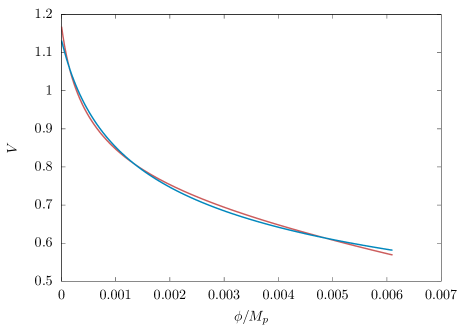
Figure 1: Figure showing the reconstructed potential $V(\phi)$ (in red) with $\phi$ when $V(a)=V_{0}a^{n}$. The blue curve shows the potential $V(\phi)=V^{\prime}_{0}(\phi+\phi_{0})^{-m}$ with $V^{\prime}_{0}=0.16$, $\phi_{0}=0.00049$ and $m=0.257$.

6 Observational Constraints

After obtaining the analytical expressions for Hubble parameter as a function of redshift (or scale factor) for different cosmological models, one can constrain its model parameters using the observational probes in the cosmology. The observational probes utilized for the data analysis includes the Type 1a Supernovae, Baryon Acoustic oscillations and Hubble parameter data sets. We constrain the parameters by employing the $\chi^{2}$ statistics. The total likelihood function for the joint data is given by,

$$\mathcal{L}_{tot}(\theta)=e^{-\chi_{tot}^{2}(\theta)\big{/}2}$$ (41)

where

$$\chi_{\rm tot}^{2}=\chi_{\rm SN}^{2}+\chi_{\rm Hub}^{2}+\chi_{\rm BAO}^{2}\,,$$ (42)

where $\theta$ denotes the parameters of the model under consideration. The best fit values of the model parameters($\theta$) are the values corresponding to the minimum $\chi^{2}$ value.

6.1 Observational Probes

6.1.1 Hubble Data (H).

The Hubble parameter data set consists of measurements of the Hubble parameter $H(z)$ at different redshifts. We use $H(z)$ data which is compiled and listed in Table-1 of (Farooq et al., 2017). The table contains 38 measurements of Hubble parameter and its associated errors in measurements up to a redshift of z= 2.36. From the total of 38 data sets, we have considered only 32 points as we do not consider three data points taken from Alam et. al.(2016) at reshifts z= 0.38, 0.51, 0.61 and we also removed the data points corresponding to the redshits z= 0.44, 0.6, 0.72 as they are already included in the BAO dataset. The chi-squared function of Hubble data is given by,

$$\chi_{\rm Hub}^{2}(\theta)=\sum_{i=1}^{32}\frac{\left[H_{\rm th}(z_{i},\theta)-H_{\rm obs}(z_{i})\right]^{2}}{\sigma^{2}_{H}(z_{i})}\,,$$ (43)

were $\sigma_{H}$ is the error associated with each measurements.

6.1.2 Type Ia Supernovae (SN Ia).

The Type 1a supernovae are the result of the explosion of a white dwarf star in a binary when it crosses the Chandrasekhar limit. These Type 1a supernovae is an ideal probe for the study of the cosmological expansion. As they all have the same luminosity, they are considered as a good standard candle. So the first data set which we used for the analysis is the Type 1a Supernovae data from the Pantheon compilation (Scolnic et al., 2018). This data set consists of 1048 supernovae in the redshift range $0.01<z<2.26$ .

The luminosity distance of a Type 1a supernova at given redshift $z$ reads as,

$$D_{L}(z)=(1+z)\int_{0}^{z}\frac{H_{0}dz^{\prime}}{H(z^{\prime})}.$$ (44)

Moreover the luminosity distance is directly related to the observed quantity, distance modulus $\mu(z)$ given by,

$$\mu(z)=m-M=5\log D_{L}(z)+\mu_{0}$$ (45)

where $M$ and $m$ are the absolute and apparent magnitude of the supernovae. Here the quantity $\mu_{0}=5\log\left(\frac{H_{0}^{-1}}{\rm Mpc}\right)+25$ is a nuisance parameter which should be marginalized.

So for the case of SN1a, the $\chi^{2}_{SN}$ estimator is defined as,

$$\chi_{\rm SN}^{2}(\mu_{0},\theta)=\sum_{i=1}^{1048}\frac{\left[\mu_{th}(z_{i},\mu_{0},\theta)-\mu_{obs}(z_{i})\right]^{2}}{\sigma^{2}_{\mu}(z_{i})}\,,$$ (46)

where $\mu_{th}$, $\mu_{obs}$ and $\sigma_{\mu}$ are the theoretical, observed distance modulus and the unertainty in the observed quantity respectively. Here $\theta$ represents the parameters of the model under consideration. After marginalizing $\mu_{0}$ and by following the reference (Nesseris & Perivolaropoulos, 2005), we get

$$\chi_{\rm SN}^{2}(\theta)=A(\theta)-\frac{B^{2}(\theta)}{C(\theta)}\,,$$ (47)

where,

$$\,\,A(\theta)=\sum_{i=1}^{1048}\frac{\left[\mu_{th}(z_{i},\mu_{0}=0,\theta)-\mu_{obs}(z_{i})\right]^{2}}{\sigma^{2}_{\mu}(z_{i})}\,,\\$$ (48)

$$B(\theta)=\sum_{i=1}^{1048}\frac{\mu_{th}(z_{i},\mu_{0}=0,\theta)-\mu_{obs}(z_{i})}{\sigma^{2}_{\mu}(z_{i})}\,,$$ (49)

$$C(\theta)=\sum_{i=1}^{1048}\frac{1}{\sigma^{2}_{\mu}(z_{i})}\,.$$ (50)

6.1.3 Baryon Acoustic Oscillations (BAO).

The Baryon Acoustic Oscillations (BAO), which are considered as the standard rulers of the cosmology, are frozen relics left over from the pre-decoupling universe. Here we have used the BAO data from 6dFGS, SDSS DR7 and WiggleZ at redshifts z = 0.106, 0.2, 0.35, 0.44, 0.6 and 0.73. In order to derive the BAO constraints we make use of the Distance parameter $D_{v}(z)$ which is a function of angular diameter distance and Hubble parameter given by,

$$D_{v}(z)=\Big{[}(1+z)^{2}d^{2}_{A}(z)\frac{z}{H(z)}\Big{]}^{\frac{1}{3}}$$ (51)

Here $d_{A}(z)$ is the angular diameter distance. We use the measurements of acoustic prameter $A(z)$ from (Blake et al., 2011), where the theoretically predicted $A_{th}(z)$ is given by Eq. 5 of (Eisenstein et al., 2005).

$$A_{th}(z)=\frac{100D_{v}(z)\sqrt{\Omega_{m0}h^{2}}}{z}$$ (52)

After following the procedures given in Sec. 5.4 of (Omer Farooq, 2013), one can obtain the acoustic parameter $A_{th}$ independent of the Hubble constant $H_{0}$. Finally after some algebra the chi-squared function of BAO data (Blake et al., 2011) reads as,

$$\chi_{\rm BAO}^{2}(\theta)=\sum_{i=1}^{6}\frac{\left[A_{th}(z_{i},\theta)-A_{obs}(z_{i})\right]^{2}}{\sigma^{2}_{A}(z_{i})}\,,$$ (53)

Parameter	Prior
$\Omega_{m0}$	[0, 1]
$V_{0}$	[0, 1]
$n$	[-5, 5]
$H_{0}$	[55, 80]

Table 1: Priors used for the MCMC analysis of the power law potential, $V_{0}a^{n}$.

6.2 Methodology

We used the Markov Chain Monte Carlo (MCMC) method to find the high confidence regions of the model parameters given a set of observational data . We perform a likelihood analysis to minimize the $\chi^{2}$ function in Eq. 42 and thereby obtain the best-fit model parameters corresponding to the minimum $\chi^{2}$ value. The minimization of the $\chi^{2}$ is equivalent to the maximization of the likelihood function in Eq. 41. Here we constrain the parameters of the power law potential given in Sec. 3.1. The model parameters and their prior values considered for the MCMC analysis is given in Table 1.

Initially, we begin the MCMC analysis with the usual way where we consider a simple proposal function of the form, $\theta^{j}_{i+1}=\theta^{j}_{i}+\delta\theta^{j}\eta^{j}$, where $j$ is a parameter index, $\delta^{j}$ is a predefined rms step size, and $\eta^{j}$ is a Gaussian stochastic variate of zero mean and unit variance. As we are dealing with a model of five parameters, most of the parameters of interest will be strongly correlated and make this choice quite inefficient. So we performed certain optimization on the MCMC chain samples, which enables us to increase the acceptance ratio and also the chain convergence. After obtaining sufficient samples from the preliminary chain, we check the autocorrelation of the Markov chain. This will give us an idea for estimating how many iterations of the Markov chain are needed for effectively independent samples. Later we perform thinning on the initial chain we had already obtained so as to get less correlated samples. This action will further reduce the total number of samples. We will then compute the covariance matrix $C_{ij}=\big{<}\delta\theta^{i}\delta\theta^{j}\big{>}$of the resulting samples. Finally, we then Cholesky-decompose this matrix, $\mathbb{C}=\mathbb{L}\mathbb{L}^{t}$ where $\mathbb{C}$ is the covariance matrix, $\mathbb{L}$ and $\mathbb{L}^{t}$ are the lower triangular matrix and its conjugate transpose respectively. We then redefine our proposal function to be $\theta_{i+1}=\theta_{i}+\alpha\mathbb{L}\mathbb{\eta}$, where $\eta$ is now a vector of Gaussian variates and $\alpha$ is an overall scale factor, typically initialized at $\sim 0.3$. This will help us to have the proposed samples with approximately correct covariance structure, and it will also improve the sampling efficiency significantly. In order to avoid very high and very small step sizes, we also impose a constraint that the acceptance ratio must be higher than $5\%$ and lower than $80\%$. One can adjust the scale factor $\alpha$ if one of these two criteria is violated.

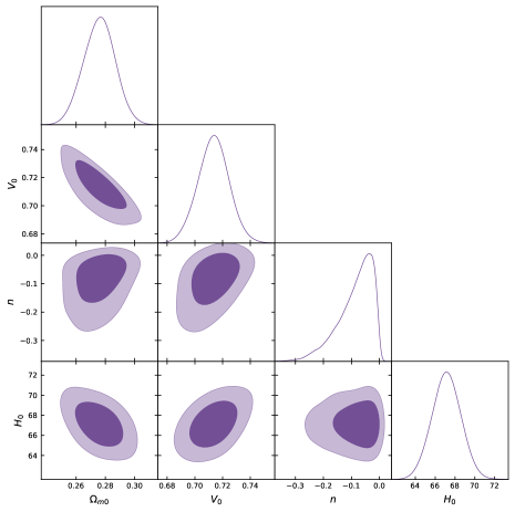
Figure 2: Posterior distribution for the model parameters ($\Omega_{m0},V_{0},n,H_{0}$) of the power law potential. The contours shows 68.3% and 95.5% confidence regions. The quantitative results are summerised in Table 2.

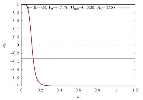
Figure 3: Figure showing the variation of $\omega_{\phi}$ as a function of scale factor corresponding to the best-fit values of the power law potential.

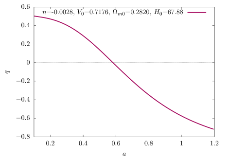
Figure 4: Figure showing the variation of deceleration parameter as a function of scale factor corresponding to the best-fit values of the power law potential. .

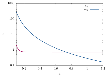
Figure 5: Figure showing the variation of energy density (log scale) of scalar field and non-relativistic matter as a function of scale factor corresponding to the best-fit values of the power law potential. .

Parameter	Best-fit $\pm$	Mean $\pm$
	95.5% limits	95.5% limits
$\Omega_{m0}$	$0.2820^{+0.029}_{-0.034}$	$0.276\pm 0.021$
$V_{0}$	$0.7176^{+0.029}_{-0.038}$	$0.713\pm 0.022$
$n$	$-0.0028^{+0.006}_{-0.324}$	$-0.085^{+0.090}_{-0.13}$
$H_{0}$	$67.88^{+4.48}_{-4.60}$	$67.1\pm 2.9$
$\chi^{2}_{min}=1054.0437$

Table 2: Best fit model for the power law Potential.

7 Discussions and Conclusions

The exact solutions of Einstein’s equations play a very important role in cosmology as they help in the understanding of quantitative and qualitative features of the dynamics of the universe as a whole. In this article, we discuss a method to obtain analytical expressions for the equation of state parameter, deceleration parameter and Hubble parameter in spatially flat FRW model of the universe with a perfect fluid and scalar field.

In Sec. 2 a method is proposed to obtain analytical expressions for the kinetic energy ($\dot{\phi^{2}}$) of the scalar field as a function of scale factor for different choices of the scalar field potential. Once the kinetic term ($\dot{\phi^{2}}$) is obtained, one can also obtain exact solutions for $\omega_{\phi}$, $\omega_{tot}$, $q$ and $H(a)$ by simple substitution. The method proposed in this article can also be applied to inflationary phase, to obtain analytical solutions, where the scalar field dominates. The effective equation of state parameter $\omega_{tot}$ and also the deceleration parameter are of great importance as they provide information about the epochs of acceleration and deceleration phases of the universe.

It is important to emphasize the importance of exact expression of $H(a)$ (or $H(z)$) obtained by us in scalar field cosmology with other perfect fluid components like matter and radiation. The analytical results can be directly fitted with observations of $H(z)$ to estimate the best-fit values of parameters of the theory. Thus our method builds an important connection between theory and observations to constrain the scalar field potential along with other cosmological parameters.

In Sec. 4, we consider the inverse problem of reconstructing the scalar field potential energy by assuming any general analytical expression of scalar field equation of state parameter as a function of the scale factor. By this method, we also reconstructed the scalar field potential for one of the most widely used parametrizations of dark energy called the Chevallier-Polarski-Linder (CPL) model.

Another important result that can be obtained using the results of this article, is to reconstruct the scalar field potential in terms of scalar field. In Sec. 5 we have discussed the method of reconstruction of $V(\phi)$ from the assumed model of $V(a)$ and the exact analytical expressions of $\dot{\phi}(a)$, $H(a)$ and using simple numerical integration. Thus we obtained that the potential $V(a)=V_{0}a^{n}$ has a close resemblance to the class of quintessential tracker potentials proposed by Ratra and Peebles in 1988.

Finally in Sec. 6 we constrained the model parameters of the power law potential with the Hubble parameter data, Baryon Acoustic Oscillation(BAO) data and the recent Panthelon Type 1a supernovae Compilation. The contours showing the 68.3% and 98.5% confidence regions are depicted in Fig. 2. The best-fit and the mean values are shown in Table 2. Interestingly, we observed that the $H_{0}=67.1\pm 1.5\,Km/S/M_{pc}$ value we obtained with low redshift data is consistent with the high redshift CMB observations($H_{0}=67.4\pm 0.5\,Km/S/M_{pc}$) at one sigma (Planck Collaboration et al. (2020)).We also explored the late-time evolution of the universe corresponding to the best-fit model parameters. Although, the formalism of this article is capable also for early scalar field dominated inflation, in the current work we focus on the study of the late time acceleration of the universe. For our analysis, we therefore, choose the scale factor between $a=0.1$ and $a=1.2$ which includes the current epoch $a_{0}=1$.

The variation of equation of state parameter $\omega_{\phi}$ and deceleration parameter $q(a)$ for the best-fit parameters are shown in Fig. 3 and  4. From the Fig. 3, we can see that the present value($a=1$) of the equation of state parameter of the scalar field can go as low as $\omega_{\phi}=-0.9999$. Thus at the present epoch, the scalar field behaves just like a cosmological constant. This is because within two sigma limits the best-fit value of the power ’$n$’ is consistent with zero, see Table 2, which gives a constant scalar field potential. Moreover, the transition between the deceleration to the accelerated phases of expansion occurs at $a\sim 0.6$ which is also shown in Fig. 4. The Fig. 5 shows the variation of energy density of the scalar field and the non-relativistic matter as a function of scale factor. We see that transition between matter and dark-energy dominated Universe occurs around $a\sim 0.75$, i.e., the scalar field starts to dominate at the very late stage of the evolution of the Universe and it drives the present accelerated expansion. From the Table 2, the present density parameter of the non-relativistic matter and dark energy corresponds to $\Omega_{m0}\sim 0.29$ and $\Omega_{\phi}\sim 0.71$ respectively.

The method discussed in Sec. 2 is not limited to the power law form of the potential that we have considered. It can also be applied to any other forms of potentials which are not discussed here. This method helps in finding the cosmological dynamical variables in an exact form without even knowing the evolution of scale factor. For instance, the Hubble paramter, $H(a)$ which we obtained analytically is directly observable. So the difficulty of solving coupled non-linear equations that one usually encounters while applying observational constraints in scalar field dark energy models can be alleviated.

Appendix A.

To derive Eqn. 34 using Eqn. 32 we first obtain,

$$\frac{d\dot{\phi}^{2}}{da}=2\biggl{[}\frac{dV}{da}\biggl{(}\frac{1+\omega_{\phi}}{1-\omega_{\phi}}\biggr{)}+V\bigg{\{}\frac{1}{1-\omega_{\phi}}+\frac{1+\omega_{\phi}}{\bigl{(}1-\omega_{\phi}\bigr{)}^{2}}\biggr{\}}\frac{d\omega_{\phi}}{da}\biggr{]}\,,$$ (54)

which can be simplified as,

$$\frac{d\dot{\phi}^{2}}{da}=\frac{2V}{\bigl{(}1-\omega_{\phi}\bigr{)}^{2}}\frac{d\omega_{\phi}}{da}+2\frac{dV}{da}\biggl{(}\frac{1+\omega_{\phi}}{1-\omega_{\phi}}\biggr{)}\,.$$ (55)

Using Eqn. 55 in Eqn. 9 and rearranging terms we obtain,

$$\begin{split}\frac{dV}{da}\biggl{[}1+\frac{1+\omega_{\phi}}{1-\omega_{\phi}}\biggr{]}+\\ &V\biggl{[}\frac{6}{a}\frac{\bigl{(}1+\omega_{\phi}\bigr{)}}{\bigl{(}1-\omega_{\phi}\bigr{)}}+\frac{1}{\bigl{(}1-\omega_{\phi}\bigr{)}^{2}}\frac{d\omega_{\phi}}{da}\biggr{]}&=0\,,\end{split}$$ (56)

which can be easily simplified into the form of Eqn. 34.

References

- Andrianov et al. (2011) Andrianov, A. A., Cannata, F., & Kamenshchik, A. Y. 2011, JCAP, 2011, 004. doi:10.1088/1475-7516/2011/10/004
- Bamba et al. (2012) Bamba, K., Capozziello, S., Nojiri, S., et al. 2012, ApSS, 342, 155. doi:10.1007/s10509-012-1181-8
- Barrow & Paliathanasis (2016) Barrow, J. D. & Paliathanasis, A. 2016, Phys. Rev. D , 94, 083518. doi:10.1103/PhysRevD.94.083518
- Barrow & Paliathanasis (2016) Barrow, J. D. & Paliathanasis, A. 2016, arXiv:1611.06680
- Barrow & Paliathanasis (2018) Barrow, J. D. & Paliathanasis, A. 2018, European Physical Journal C, 78, 767. doi:10.1140/epjc/s10052-018-6245-7
- Barrow & Saich (1993) Barrow, J. D. & Saich, P. 1993, Classical and Quantum Gravity, 10, 279. doi:10.1088/0264-9381/10/2/009
- Barrow (1990) Barrow, J. D. 1990, Physics Letters B, 235, 40
- Barrow (1993) Barrow, J. D. 1993, Phys. Rev. D , 48, 1585. doi:10.1103/PhysRevD.48.1585
- Basilakos & Plionis (2010) Basilakos, S. & Plionis, M. 2010, Astroph. J. Lett., 714, L185. doi:10.1088/2041-8205/714/2/L185
- Blake et al. (2011) Blake, C., Kazin, E. A., Beutler, F., et al. 2011, Mon. Not. Roy. Ast. Soc. , 418, 1707. doi:10.1111/j.1365-2966.2011.19592.x
- Capozziello & Roshan (2013) Capozziello, S. & Roshan, M. 2013, Physics Letters B, 726, 471. doi:10.1016/j.physletb.2013.08.047
- Chakrabarti (2017) Chakrabarti, S. 2017, General Relativity and Gravitation, 49, 24. doi:10.1007/s10714-017-2186-y
- Charters & Mimoso (2010) Charters, T. & Mimoso, J. P. 2010, JCAP, 2010, 022. doi:10.1088/1475-7516/2010/08/022
- Chervon et al. (2018) Chervon, S. V., Fomin, I. V., & Beesham, A. 2018, European Physical Journal C, 78, 301. doi:10.1140/epjc/s10052-018-5795-z
- Chimento & Jakubi (1996) Chimento, L. P. & Jakubi, A. S. 1996, International Journal of Modern Physics D, 5, 71. doi:10.1142/S0218271896000084
- Chimento et al. (2013) Chimento, L. P., Forte, M., & Richarte, M. G. 2013, Modern Physics Letters A, 28, 1250235. doi:10.1142/S0217732312502355
- Copeland et al. (1993) Copeland, E. J., Kolb, E. W., Liddle, A. R., et al. 1993, Phys. Rev. D , 48, 2529. doi:10.1103/PhysRevD.48.2529
- Davis et al. (2007) Davis, T. M., Mörtsell, E., Sollerman, J., et al. 2007, Astroph. J. , 666, 716. doi:10.1086/519988
- de Ritis et al. (1990) de Ritis, R., Marmo, G., Platania, G., et al. 1990, Phys. Rev. D , 42, 1091. doi:10.1103/PhysRevD.42.1091
- Dimakis et al. (2016) Dimakis, N., Karagiorgos, A., Zampeli, A., et al. 2016, Phys. Rev. D , 93, 123518. doi:10.1103/PhysRevD.93.123518
- Eisenstein et al. (2005) Eisenstein, D. J., Zehavi, I., Hogg, D. W., et al. 2005, Astroph. J. , 633, 560. doi:10.1086/466512
- Elizalde et al. (2004) Elizalde, E., Nojiri, S., & Odintsov, S. D. 2004, Phys. Rev. D , 70, 043539. doi:10.1103/PhysRevD.70.043539
- Elizalde et al. (2008) Elizalde, E., Nojiri, S., Odintsov, S. D., et al. 2008, Phys. Rev. D , 77, 106005. doi:10.1103/PhysRevD.77.106005
- Ellis & Madsen (1991) Ellis, G. F. R. & Madsen, M. S. 1991, Classical and Quantum Gravity, 8, 667. doi:10.1088/0264-9381/8/4/012
- Farooq et al. (2017) Farooq, O., Ranjeet Madiyar, F., Crandall, S., et al. 2017, Astroph. J. , 835, 26. doi:10.3847/1538-4357/835/1/26
- Fomin (2018) Fomin, I. V. 2018, Russian Physics Journal, 61, 843. doi:10.1007/s11182-018-1468-5
- Guth (1981) Guth, A. H. 1981, Phys. Rev. D , 23, 347. doi:10.1103/PhysRevD.23.347
- Guzmán et al. (2007) Guzmán, W., Sabido, M., Socorro, J., et al. 2007, International Journal of Modern Physics D, 16, 641. doi:10.1142/S0218271807009401
- Harko et al. (2014) Harko, T., Lobo, F. S. N., & Mak, M. K. 2014, European Physical Journal C, 74, 2784. doi:10.1140/epjc/s10052-014-2784-8
- Hicken et al. (2009) Hicken, M., Wood-Vasey, W. M., Blondin, S., et al. 2009, Astroph. J. , 700, 1097. doi:10.1088/0004-637X/700/2/1097
- Hinshaw et al. (2009) Hinshaw, G., Weiland, J. L., Hill, R. S., et al. 2009, ApJS, 180, 225. doi:10.1088/0067-0049/180/2/225
- Komatsu et al. (2009) Komatsu, E., Dunkley, J., Nolta, M. R., et al. 2009, ApJS, 180, 330. doi:10.1088/0067-0049/180/2/330
- Komatsu et al. (2011) Komatsu, E., Smith, K. M., Dunkley, J., et al. 2011, ApJS, 192, 18. doi:10.1088/0067-0049/192/2/18
- Kowalski et al. (2008) Kowalski, M., Rubin, D., Aldering, G., et al. 2008, Astroph. J. , 686, 749. doi:10.1086/589937
- Kruger & Norbury (2000) Kruger, A. T. & Norbury, J. W. 2000, Phys. Rev. D , 61, 087303. doi:10.1103/PhysRevD.61.087303
- Liddle & Turner (1994) Liddle, A. R. & Turner, M. S. 1994, Phys. Rev. D , 50, 758. doi:10.1103/PhysRevD.50.758
- Liddle & Scherrer (1999) Liddle, A. R. & Scherrer, R. J. 1999, Phys. Rev. D , 59, 023509. doi:10.1103/PhysRevD.59.023509
- Lima & Alcaniz (2000) Lima, J. A. S. & Alcaniz, J. S. 2000, Mon. Not. Roy. Ast. Soc. , 317, 893. doi:10.1046/j.1365-8711.2000.03695.x
- Lima et al. (2009) Lima, J. A. S., Jesus, J. F., & Cunha, J. V. 2009, Astroph. J. Lett., 690, L85. doi:10.1088/0004-637X/690/1/L85
- Linde (1983) Linde, A. D. 1983, Physics Letters B, 129, 177. doi:10.1016/0370-2693(83)90837-7
- Linde (1982) Linde, A. D. 1982, Physics Letters B, 108, 389. doi:10.1016/0370-2693(82)91219-9
- Linde (2005) Linde, A. 2005, hep-th/0503203
- Muslimov (1990) Muslimov, A. G. 1990, Classical and Quantum Gravity, 7, 231. doi:10.1088/0264-9381/7/2/015
- Nesseris & Perivolaropoulos (2005) Nesseris, S. & Perivolaropoulos, L. 2005, Phys. Rev. D , 72, 123519. doi:10.1103/PhysRevD.72.123519
- Omer Farooq (2013) Omer Farooq, M. 2013, arXiv:1309.3710
- Paliathanasis et al. (2014) Paliathanasis, A., Tsamparlis, M., & Basilakos, S. 2014, Phys. Rev. D , 90, 103524. doi:10.1103/PhysRevD.90.103524
- Paliathanasis et al. (2015) Paliathanasis, A., Tsamparlis, M., Basilakos, S., et al. 2015, Phys. Rev. D , 91, 123535. doi:10.1103/PhysRevD.91.123535
- Peebles & Ratra (2003) Peebles, P. J. & Ratra, B. 2003, Reviews of Modern Physics, 75, 559. doi:10.1103/RevModPhys.75.559
- Perlmutter et al. (1999) Perlmutter, S., Aldering, G., Goldhaber, G., et al. 1999, Astroph. J. , 517, 565. doi:10.1086/307221
- Planck Collaboration et al. (2020) Planck Collaboration, Aghanim, N., Akrami, Y., et al. 2020, AAp, 641, A6. doi:10.1051/0004-6361/201833910
- Planck Collaboration et al. (2014) Planck Collaboration, Ade, P. A. R., Aghanim, N., et al. 2014, AAp, 571, A16. doi:10.1051/0004-6361/201321591
- Ratra & Peebles (1988) Ratra, B. & Peebles, P. J. E. 1988, Phys. Rev. D , 37, 3406. doi:10.1103/PhysRevD.37.3406
- Riess et al. (1998) Riess, A. G., Filippenko, A. V., Challis, P., et al. 1998, Astron. J. , 116, 1009. doi:10.1086/300499
- Salopek & Bond (1990) Salopek, D. S. & Bond, J. R. 1990, Phys. Rev. D , 42, 3936. doi:10.1103/PhysRevD.42.3936
- Scolnic et al. (2018) Scolnic, D. M., Jones, D. O., Rest, A., et al. 2018, Astroph. J. , 859, 101. doi:10.3847/1538-4357/aab9bb
- Socorro et al. (2015) Socorro, J., D’oleire, M., & Pimentel, L. O. 2015, ApSS, 360, 20. doi:10.1007/s10509-015-2528-8
- Spergel et al. (2007) Spergel, D. N., Bean, R., Doré, O., et al. 2007, ApJS, 170, 377. doi:10.1086/513700
- Tegmark et al. (2004) Tegmark, M., Blanton, M. R., Strauss, M. A., et al. 2004, Astroph. J. , 606, 702. doi:10.1086/382125
- Yurov & Yurov (2010) Yurov, A. V. & Yurov, V. A. 2010, Journal of Mathematical Physics, 51, 082503. doi:10.1063/1.3460856
- Zhuravlev et al. (1998) Zhuravlev, V. M., Chervon, S. V., & Shchigolev, V. K. 1998, Soviet Journal of Experimental and Theoretical Physics, 87, 223. doi:10.1134/1.558649