A Dual Approach for Positive T–S Fuzzy Controller Design and Its Application to Cancer Treatment Under Immunotherapy and Chemotherapy

Abstract

This study proposes an effective positive control design strategy for cancer treatment by resorting to the combination of immunotherapy and chemotherapy. The treatment objective is to transfer the initial number of tumor cells and immune–competent cells from the malignant region into the region of benign growth where the immune system can inhibit tumor growth. In order to achieve this goal, a new modeling strategy is used that is based on Takagi–Sugen. A Takagi-Sugeno fuzzy model is derived based on the Stepanova nonlinear model that enables a systematic design of the controller. Then, a positive Parallel Distributed Compensation controller is proposed based on a linear co-positive Lyapunov Function so that the tumor volume and administration of the chemotherapeutic and immunotherapeutic drugs is reduced, while the density of the immune-competent cells is reached to an acceptable level. Thanks to the proposed strategy, the entire control design is formulated as a Linear Programming problem, which can be solved very efficiently. Finally, the simulation results show the effectiveness of the proposed control approach for the cancer treatment.

1 Introduction

After cardiovascular disease, cancer is the most common cause of death in the world [1]. There are several therapies for the cancer treatment such as surgery, immunotherapy, radiotherapy, and chemotherapy. It is noticeable that even when the treatment is completed, there is still a possibility of the disease. For this reason, many researchers have studied the cancer models, aiming to find a definitive cancer treatment [2, 3, 4]. In the literature, chemotherapy is the most common way for the cancer treatment. In some cases, chemotherapy is the only treatment. However chemotherapy is mostly used along with other treatments, the main reasons for this are described as follows: i) cancer cells tend to grow fast, and chemotherapy drugs kill fast-growing cells. Since these drugs travel throughout the body, they can also affect normal and healthy cells that are fast-growing. Therefore, damage to healthy cells is the main side effect of the chemotherapy. ii) cancer cells are deforming in order to survive while under treatment, and for this reason, the chemotherapy treatment is often stopped. In the last few decades, immunotherapy has become an important part of treating some types of cancers [5]. This treatment uses the body’s own immune system to cure cancer with fewer side effects compared to the chemotherapy treatment. As a result, the optimal way to blend manifold cancer treatments remains an open problem.

Abundant efforts have been devoted to study the dynamics and interactions of the tumor and normal cells aiming to design appropriate control strategies, such that the tumor cells are eradicated as much as possible without harming the healthy cells. Stepanova [6] suggested a mathematical model for expressing the interactions between the tumor and immune system. This model, in spite of its simplicity, and with a small number of parameters, plays an important role in resembling tumor-immune interactions. In [7], a metamodel for tumor-immune system interactions has been proposed, where the treatment has been formulated as an optimal control problem by cytotoxic agents and immunostimulations. In [8], a multi-objective optimal control of a tumor growth model with the immune response and drug therapies has been presented, so that the average number of tumor cells and immuno and chemotherapeutic drugs administration are minimized at the same time. In [9], a comparison has been made by means of an optimal strategy to control the dynamics of three tumor growth models that consist of an immune system and drug administration therapy.

Up to now, most of the control strategies are based on minimizing the drug dosage in an open-loop mode using an optimal control approach. Model predictive control (MPC) has been applied as an effective strategy for the cancer chemotherapy [10]. Blended immunotherapy and chemotherapy for tumor treatment using MPC has been proposed in [11]. The Kirschner model has been proposed in [12], and adopted to design an adaptive fuzzy back-stepping control strategy for the tumor-immune system in [13]. The purpose of this work is to develop an effective treatment plan for the drug dosage to reduce the volume of tumor cells. However, this case only covers cancer immunotherapy.

In the past two decades, significant advances have been made for the control of nonlinear systems. Takagi–Sugeno (T–S) fuzzy models have widely used in the control community to design nonlinear control strategies [14, 15, 16]. This model consists of a convex combination of several linear subsystems and nonlinear membership functions in the form of IF-THEN rules, which are considered as a universal approximator for nonlinear dynamics.

This work considers the reformed Stepanova model for the cancer-immune system interactions. Although this model is a simple and basic model, it includes many important medical features. The state variables in this model involve quantities that have non-negative signs. This model belongs to a significant class of systems known as “Positive Systems”. In such systems, the state variables that correspond to any non-negative initial states always have to be non-negative [17, 18]. In addition, the positive systems states are defined inside a cone situated in the positive orthant instead of the whole space. Such systems have several applications in controlling chemical processes, biology, medicine, and economics systems [19].

This paper is a mixture of immunotherapy and chemotherapy for the cancer treatment. The purpose of this research is to design a positive T–S fuzzy controller for an appropriate and efficient treatment, in which the combination of tumor volume as well as the potential side effects are reduced, and, consequently, the density of immune–competent cells is reached to an admissible level. Simulation results show the effectiveness of the proposed method, which can help to develop mixed therapies. Compared to the state-of-the-art approaches, it is observed that during this treatment the maximum number of cancer cells and the side effects are significantly reduced.

The main contributions of this paper can be summarized as follows: a new fuzzy modeling framework, which exactly represents the nonlinear system, is proposed, which reduces the number of fuzzy rules that inherently affect the conservatism. Then, a parallel distributed compensation (PDC) is derived as a naive and reliable method to handle nonlinear control systems. The concept of a dual system is also employed. The previous methods to stabilize the positive systems use a quadratic Lyapunov function that is imposed to be diagonal, and, consequently, increases conservatism. Here, a linear co-positive Lyapunov function (LCPLF) is proposed. The obtained results are expressed in terms of linear programming (LP) that leads to more convenient conditions for computation and analysis compared to the existing ones. However, the fuzzy model cannot be easily extracted from the reformed Stepanova model due to the existence of a constant term in the nonlinear model. To cope with this problem, this approach considers the control input has two parts; one part of this control agent eliminates some nonlinear terms, and the other part is responsible for the stability of the remaining nonlinear system.

The rest of the paper is organized as follows: The Stepanova model of the tumor-immune system is described in Section 2. The proposed fuzzy modeling framework and the proposed control method for the positive T–S system are presented in Section 3. The simulation results are presented in Section 4. Section 5 concludes the paper.

Notations: $\mathbb{R}^{n}$ represents a set of n-column real vectors, and $\mathbb{R}^{n\times m}$ is a set of $n\times m$ real matrix. The notation $A\geq\geq B$ (respectively, $A\gg B$) means that the matrix $A-B$ is element-wise nonnegative (respectively, $A-B$ is element-wise positive). $\textbf{1}=[1,1,...,1]^{T}$ denotes a column vector, in which all entries are equal to 1. The superscript ‘$T$’ stands for the transpose operator; $I$ and $0$ represent the identity and zero matrices, respectively; diag$(A_{1},...,A_{n})$ represents a block diagonal matrix, in which $A_{1},...,A_{n}$ are square matrices along the main diagonal.

2 Stepanova Model

In this section, the Stepanova mathematical model that expresses the interactions between the immune and tumor system is introduced [6]. Here the Stepanova model is used to describe the tumor growth with an immune response, immunotherapy, and chemotherapy. To clarify this subject, one can consider the reformed form of the Stepanova model as follows [7]:

$$\dot{x}_{1}(t) =\mu_{c}x_{1}(t)F(x_{1})-\gamma x_{1}(t)x_{2}(t)-k_{x_{1}}x_{1}(t)u_{1}(t)$$ (1)

$$\dot{x}_{2}(t) =\mu_{I}(x_{1}(t)-\beta x_{1}^{2}(t))x_{2}(t)-\delta x_{2}(t)+\alpha+k_{x_{2}}x_{2}(t)u_{2}(t)$$ (2)

where $x_{1}(t)$ and $x_{2}(t)$ indicate the number of tumor cells and effector cells of the immune system, respectively. The control agent $u_{1}(t)$ denotes the blood profiles of a cytotoxic agent and $u_{2}(t)$ indicates the immune system booster drug for the immune cells in the cancer treatment. $k_{x_{1}}$ and $k_{x_{2}}$ stand for the maximum dose rates of the therapeutic agents.

Equation (1) models tumor growth, where $\mu_{c}$ denotes the tumor growth coefficient and the coefficient $\gamma$ shows the rate at which cancer cells are eliminated. The term $\gamma x_{1}x_{2}$ models the useful effect of the immune response on the cancer volume. $F$ is a function of the growth of the tumor cells and there are various selections that can be considered for that. However, here the Gompertz growth function [20] in the form of $F(x_{1})=-ln(\frac{x_{1}(t)}{x_{\infty}})$ is considered instead of other growth functions such as exponential model or logistic or generalized logistic growth. In this function, $x_{\infty}$ is the fixed finite carrying capacity of the tumor.

Equation (2) models the main specifications of the immune system’s response to the tumor cells. The effect of the tumor growth on the activity of immune cells is shown by the first term. The coefficients $\mu_{I}$, $\beta$ and $\delta$ are the tumor stimulated proliferation rate, the inverse threshold for tumor suppression and the rate of natural death of immune cells, respectively. $\alpha$ represents the rate of influx of the effector cells from the primary organs.

Equilibrium point: The determination of the equilibrium points and analyzing systems behavior around these points play a significant role in dynamical systems. Stopping the growth and moving process in these points are some of the most important reasons behind this subject. Although this is not suitable for some physical processes such as motion, it can be an ideal solution for some medical applications, such as tumor growth [21].

When the patient’s body system reaches a point, in which the number of tumor cells is zero or very low, the treatment is completed. The unforced system without medication has two locally asymptotically stable equilibriums, which can be obtained by solving the equations $\dot{x}_{1}(t)=0$ and $\dot{x}_{2}(t)=0$, one microscopic point at (72.961, 1.32), which is the region of attraction corresponding to the benign conditions (where the number of tumor cells is low) and the other is macroscopic point at (737.278, 0.032), which is the region of attraction related to the malignant situations, where the number of tumor cells is high. These regions of attraction are separated by a stable manifold of an intermediate saddle point at (356.2, 0.439).

It is obvious that for any model of cancer, the states $x_{1}(t)$ and $x_{2}(t)$ should remain positive for the positive initial conditions ${x_{1}}(0)$ and ${x_{2}(0)}$, and arbitrary acceptable controls $u_{1}(t)$ and $u_{2}(t)$. Therefore, the nonlinear model mentioned for cancer, based on the interaction between the tumor cells and the immune cells, can be considered as a positive system. Therefore, a set $\kappa$ that can be defined as follow is a positive invariant set for the above model, and, then, no positive constraints imposed to variables:

$$\kappa=\left\{(x_{1},x_{2}):x_{1}>0,x_{2}>0\right\}.$$

3 Positive T-S Fuzzy Modeling and Controller design

In this section, first, a new fuzzy modeling framework for the nonlinear model of the cancer treatment is proposed so that the number of fuzzy rules is reduced. Next, the stability and new LP conditions for the controller design of positive T–S systems are proposed.

3.1 Fuzzy Modeling

To obtain a T–S fuzzy representation of Eqs. (1) and (2), the nonlinear terms of the model are considered as premise variables. Denote $\vartheta_{1}=-\mu_{c}ln(\dfrac{x_{1}}{x_{\infty}})$, $\vartheta_{2}=-\gamma x_{1}$, $\vartheta_{3}=\mu_{I}(x_{1}-\beta x_{1}^{2})-\delta$, $\vartheta_{4}=-k_{x_{1}}x_{1}$ and, $\vartheta_{5}=k_{x_{2}}x_{2}$. Therefore, the corresponding model is given by:

$$\left\{\begin{array}[]{l}\dot{x}_{1}=\vartheta_{1}x_{1}-\vartheta_{2}x_{2}-\vartheta_{4}u_{1}\\ \dot{x}_{2}=\vartheta_{3}x_{2}+\alpha+\vartheta_{5}u_{2}.\end{array}\right.$$ (5)

Because of the existence of a constant term $\alpha$ in the second equation, the fuzzy model cannot be easily extracted from the system (5). To overcome this problem, an approach is suggested, which is based on the change of variable. For this purpose, the control input consists of two parts: i) one part is used to eliminate some nonlinear terms of equations; ii) another part is considered to stabilize the reminding nonlinear dynamical model. This approach has two main advantages; First, a T–S fuzzy model can be extracted directly from nonlinear equations of the system, and secondly, the number of fuzzy rules is reduced that leads to less conservatism. Accordingly, the new control input vector is defined as follows:

$$u_{2}^{*}=\alpha+k_{x_{2}}x_{2}u_{2}\ \rightarrow\ u_{2}=\dfrac{u_{2}^{*}-\alpha}{k_{x_{2}}x_{2}}$$ (6)

Therefore, the equations (1) and (2) can be rewritten as follows:

$$\begin{cases}\dot{x}_{1}=-\mu_{c}x_{1}ln(\dfrac{x_{1}}{x_{\infty}})-\gamma x_{1}x_{2}-k_{x_{1}}x_{1}u_{1},\\ \dot{x}_{2}=\mu_{I}(x_{1}-\beta x_{1}^{2})x_{2}-\delta x_{2}+u_{2}^{*}.\end{cases}$$ (7)

By defining the nonlinear terms as $\bar{\vartheta_{1}}=-\mu_{c}ln(\dfrac{x}{x_{\infty}})-\gamma y$, $\bar{\vartheta_{2}}=-\mu_{I}(x-\beta x^{2})-\delta$ and, $\bar{\vartheta_{3}}=-k_{x}x$, then the general form of the Eq.(7) is as follows:

$$\begin{cases}\dot{X}(t)=A(\bar{\vartheta}_{1},\bar{\vartheta}_{2})X(t)+B(\bar{\vartheta}_{3})U(t),\\ \ z(t)=CX(t),\end{cases}$$ (8)

where $z(t)$ is the output vector and we have,

$$X=\begin{bmatrix}x_{1}\\ x_{2}\end{bmatrix},\ \ A(\bar{\vartheta}_{1},\bar{\vartheta}_{2})=\begin{bmatrix}\bar{\vartheta}_{1}&0\\ 0&\bar{\vartheta}_{2}\end{bmatrix},\ \ B(\bar{\vartheta}_{3})=\begin{bmatrix}\bar{\vartheta}_{3}&0\\ 0&1\end{bmatrix},\ \ U=\begin{bmatrix}u_{1}\\ u_{2}^{*}\end{bmatrix},\ \ C=\it I_{2}.$$

In the set point tracking problem, the following integral control structure is used:

$$e_{I}=\int(z_{r}-z)dt$$

where $e=z_{r}-z$ is the tracking error. The goal is that the output $z$ tracks a given reference $z_{r}$. Finally, the augmented system can be defined by the following system:

$$\begin{cases}\dot{\bar{X}}(t)=\bar{A}(\bar{\vartheta}_{1},\bar{\vartheta}_{2})\bar{X}+\bar{B}(\bar{\vartheta}_{3})U+\bar{D}Z_{r},\\ \ z(t)=\bar{C}\bar{X}.\end{cases}$$ (9)

where

$$\bar{X}=\begin{bmatrix}X\\ e_{I}\end{bmatrix} ,\ \ \bar{A}(\bar{\vartheta}_{1},\bar{\vartheta}_{2})=\begin{bmatrix}A(\bar{\vartheta}_{1},\bar{\vartheta}_{2})&0\\ -C&0\end{bmatrix},\ \ \bar{B}(\bar{\vartheta}_{3})=\begin{bmatrix}B(\bar{\vartheta}_{3})\\ 0\end{bmatrix},$$

$$\bar{C}=\begin{bmatrix}C&0\end{bmatrix},\ \ \bar{D}=\begin{bmatrix}0&0\\ 0&I\end{bmatrix},\ \ Z_{r}=\begin{bmatrix}0\\ z_{r}\end{bmatrix}.$$

By computing the maximum and minimum values of premise variables under $x_{1}\in[0,1000]$ and $x_{2}\in[0,5]$, $\bar{\vartheta_{1}}$, $\bar{\vartheta_{2}}$ and, $\bar{\vartheta_{3}}$ can be described as:

$$\bar{\vartheta}_{1} =\text{max}(\bar{\vartheta_{1}})\ .\ M_{1}(\bar{\vartheta}_{1})+\text{min}(\bar{\vartheta_{1}})\ .\ M_{2}(\bar{\vartheta}_{1}),$$

$$\bar{\vartheta}_{2} =\text{max}(\bar{\vartheta_{2}})\ .\ N_{1}(\bar{\vartheta}_{2})+\text{min}(\bar{\vartheta_{2}})\ .\ N_{2}(\bar{\vartheta}_{2}),$$

$$\bar{\vartheta}_{3} =\text{max}(\bar{\vartheta_{3}})\ .\ S_{1}(\bar{\vartheta}_{3})+\text{min}(\bar{\vartheta_{3}})\ .\ S_{2}(\bar{\vartheta}_{3}),$$

where

$$M_{1}(\bar{\vartheta_{1}})=\dfrac{\bar{\vartheta_{1}}-\text{min}(\bar{\vartheta_{1}})}{\text{max}(\bar{\vartheta_{1}})-\text{min}(\bar{\vartheta_{1}})},M_{2}(\bar{\vartheta_{1}})=1-M_{1}(\bar{\vartheta_{1}})$$

$$N_{1}(\bar{\vartheta_{2}})=\dfrac{\bar{\vartheta_{2}}-\text{min}(\bar{\vartheta_{2}})}{\text{max}(\bar{\vartheta_{2}})-\text{min}(\bar{\vartheta_{2}})},N_{2}(\bar{\vartheta_{2}})=1-N_{1}(\bar{\vartheta_{2}}),$$

$$S_{1}(\bar{\vartheta_{3}})=\dfrac{\bar{\vartheta_{3}}-\text{min}(\bar{\vartheta_{3}})}{\text{max}(\bar{\vartheta_{3}})-\text{min}(\bar{\vartheta_{3}})},S_{2}(\bar{\vartheta_{3}})=1-S_{1}(\bar{\vartheta_{3}}).$$

Accordingly, the membership functions are calculated as follows:

$$h_{1} =M_{1}\times N_{1}\times S_{1},\quad h_{2}=M_{1}\times N_{1}\times S_{2},$$

$$h_{3} =M_{1}\times N_{2}\times S_{1},\quad h_{4}=M_{1}\times N_{2}\times S_{2},$$

$$h_{5} =M_{2}\times N_{1}\times S_{1},\quad h_{6}=M_{2}\times N_{1}\times S_{2},$$

$$h_{7} =M_{2}\times N_{2}\times S_{1},\quad h_{8}=M_{2}\times N_{2}\times S_{2}.$$

It should be noted that the Euler technique is applied for discretization, however, any discretization method can also be used by a sampling time T. Hence, the T–S fuzzy model related to the augmented discrete-time system is presented by 8 linear sub-models:

$$\begin{cases}&\bar{X}(k+1)=\bar{A}d_{i}\bar{X}(k)+\bar{B}d_{i}U(k)+\bar{D}d_{i}Z_{r},\\ &z(k)=\bar{C}\bar{X}(k),\end{cases}$$ (10)

where $i=1,2,...,8$ and matrices $\bar{A}d_{i}$, $\bar{B}d_{i}$ and, $\bar{D}d_{i}$, respectively, characterize the discretized matrices related to $\bar{A}_{i}$, $\bar{B}_{i}$ and, $\bar{D}_{i}$.

To validate the newly proposed fuzzy modeling framework, the nonlinear model is simultaneously simulated with the T–S fuzzy model of the cancer system. The parameters reported in the Table (1) are used for simulation.

Table 1: The values of parameters/variables [7].

Variable/Parameter	Descriptions	Numerical value	Dimension
$x_{1}(0)$	The initial value of $x_{1}$	$600$	$10^{6}$ cells
$x_{2}(0)$	The initial value of $x_{2}$	0.1	Non-dimensional
$\alpha$	Rate of influx	0.1181	1/day
$\beta$	Inverse threshold for tumor suppression	0.00264	Non-dimensional
$\gamma$	Interaction rate	1	$10^{7}$ cells/day
$\delta$	Death rate	0.37451	$1$/day
$\mu_{C}$	Tumor growth parameter	0.5599	$10^{7}$ cells/day
$\mu_{I}$	Tumor stimulated proliferation rate	0.00484	$10^{7}$ cells/day
$x_{\infty}$	Fixed carrying capacity	780	$10^{6}$ cells
$k$	chemotherapeutic killing parameter	1	$10^{7}$ cells/day

The simulation results in the absence of control by taking an initial condition as $X_{0}=\begin{bmatrix}600&0.1\end{bmatrix}^{T}$, is shown in Fig. 1. The tumor volume is in multiples of $10^{6}$ cells, while the effector cells density is measured in a scale relative to 1. As can be seen, the behavior of both systems is quite similar and the T–S fuzzy system exactly models the nonlinear system.

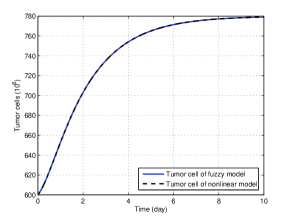
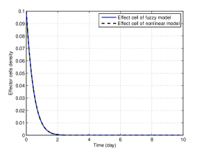
Figure 1: Dynamic profile of the tumor cells and the effector cells’ density.

Fig. 1 shows that simultaneously with the growth and proliferation of tumor cells, the density of the immune system cells decreases significantly. Therefore, these results substantiate the effectiveness of the synthesized fuzzy model that will be considered in the controller synthesis.

The goal is to design a controller that reduces the tumor volume and also holds the density of the effector cells at an acceptable level. Therefore, the controller is designed in a way that it guarantees the states $x_{1}$ and $x_{2}$ always remain positive. Then, the linear Lyapunov based method is used to design the controller that renders nonnegative states, while they do not always exist using the classical Lyapunov function even with linear matrix inequalities (LMIs).

3.2 Stability Analysis

The control objective of this subsection is to obtain the stability condition for the positive T–S fuzzy systems. The attained result is presented in the LP framework. Throughout this subsection it is assumed that the underlying system is unforced that is, $u(k)\equiv 0$.

Remark 1.

A system whose matrices are transposed is called a dual system of another one. It is significant to note that asymptotic stability of the system (33) is equivalent to asymptotic stability of its dual [22, 23], i.e,

$$x(k+1)=\sum_{i=1}^{r}h_{i}(\vartheta(k))A^{T}_{i}x(k).$$ (11)

Proposition 1.

If there exist a vector $\;p\geq\geq 0$ such that

$$(A_{i}-I)p\ll 0,$$ (12)

holds $i=1,2,...,r$, then, the system (33) is asymptotically stable.

Proof 1.

Given the positive system (11) means $x(k)\geq\geq 0$ for all $k\in R^{n}_{+}$. Consider a linear Lyapunov function candidate as

$$V(x(k))=x^{T}(k)p,\ \ p\geq\geq 0.$$ (13)

Then the rate of increase of $V(x(k))$ is given by:

$$\Delta V(x(k)) =V(x(k+1))-V(x(k)),$$

$$=x^{T}(k+1)p-x^{T}(k)p,$$

$$=\sum_{i=1}^{r}h_{i}(\vartheta(k))x^{T}(k)A_{i}p-x^{T}(k)p,$$

$$=\sum_{i=1}^{r}h_{i}(\vartheta(k))\left(x^{T}(k)(A_{i}-I)p\right)<0,$$ (14)

Since the states of positive systems are nonnegative and $0\leq h_{i}(\vartheta_{k})\leq 1$ and $\sum_{i=1}^{r}h_{i}(\vartheta(k))=1$, the Lyapunov stability condition, $\Delta V(x(k))<0$ holds if and only if the inequality (12) is satisfied. The whole proof is completed.                                 $\square$

As a conclusion, the existence of LCPLF for the dual system (11) ensures the asymptotic stability of the original system (33). It should be noted that the existence of LCPLF for the positive system (33) neither guarantees the existence of such a Lyapunov function for the dual system (11) nor ensures the correctness of the converse [22]. For example, consider the system (33) with two subsystems and the matrices:

$$A_{1}=\begin{bmatrix}1/2&1/2\\ 1/3&1/2\end{bmatrix},\quad A_{2}=\begin{bmatrix}1/2&1/2\\ 2/27&2/3\end{bmatrix}.$$

Hence, both $A_{1}$ and $A_{2}$ are nonnegative and Schur stable. It is simply seen that no LCPLF can be found, but the dual system has LCPLF $V(x(k))=\begin{bmatrix}4&3\end{bmatrix}x(k)$.

3.3 Controller synthesis for the positive T–S fuzzy system

In this subsection, an approach based on the LCPLF and PDC controller is proposed. In this technique, the concept of the dual system is used and the Lyapunov function $V(x(k))=x^{T}(k)p$ is considered to derive the stabilization condition in the form of new LPs. Assuming that the state variables can directly be measured, the main aim is then to design a state feedback controller through the PDC structure, which is defined as follows:

$$u(k)=\sum_{i=1}^{r}h_{i}(\vartheta(k))K_{i}x(k).$$ (15)

Then, the closed-loop system can be obtained by Substituting (15) into (33):

$$S_{c}:\left\{\begin{array}[]{c}x(k+1)=\sum\limits_{i=1}^{r}\sum\limits_{j=1}^{r}h_{i}(\vartheta(k))h_{j}(\vartheta(k))(A_{i}+B_{i}K_{j})x(k),\\ \ \ \ z(k)=\sum\limits_{i=1}^{r}\sum\limits_{j=1}^{r}h_{i}(\vartheta(k))h_{j}(\vartheta(k))(C_{i}+D_{i}K_{j})x(k).\end{array}\right.$$ (18)

Theorem 1.

For the positive fuzzy system (33), the state-feedback controller (15) exists such that the closed-loop system (18) is positive and asymptotically stable if and only if there exist a diagonal matrix $Q\in\mathbb{R}^{n\times n}$ and matrix $M_{j}\in\mathbb{R}^{m\times n}$ such that the following LP conditions are satisfied:

$$\left[(A_{i}-I)Q+B_{i}M_{j}\right]\textbf{1}^{n}\ll 0,\quad for\ \ i,j=1,2,...,r,$$ (19a)

$$Q\gg 0,$$ (19b)

$$M_{j}\leq\leq 0,\qquad\ \ for\quad j=1,...,r,$$ (19c)

$${{\left[{{a}^{i}}\right]}_{\,h\,t}}\,{{q}_{t}}\,+\,\sum\limits_{z=1}^{r}{\,{{\left[{{b}^{i}}\right]}_{\,h\,z}}\,{{\left[{{m}^{j}}\right]}_{\,z\,t}}}\,\geq\geq 0,\quad for\quad h,t=1,...,n.$$ (19d)

where $A_{i}\triangleq\left[a^{i}\right]_{ht},\ B_{i}\triangleq[b_{1}^{i},...,b_{n}^{i}]^{T},$ are given square matrices. Then, the controller gain $K_{j}$ is computed by:

$$K_{j}=M_{j}Q^{-1}\in\mathbb{R}^{m\times n}.$$ (20)

Proof 2.

Sufficiency: Assume that conditions (19a)-(19c) hold and $K_{j}=[k_{1}^{j},...,k_{n}^{j}]$ are defined through $k_{t}^{j}=m_{t}^{j}q_{t}$ for $j=1,..,r$ and $t=1,...,n$. Then, by replacement the fallowing inequality is obtained:

$$[(A_{i}-I)Q+B_{i}K_{j}Q]\textbf{1}^{n}\ll 0,$$

$$[(A_{i}-I)+B_{i}K_{j}]Q\textbf{1}^{n}\ll 0,$$

By definition $p\triangleq Q\textbf{1}^{n}$ and by using Proposition (1), one can conclude that the system (18) is asymptotically stable. Now, the condition (19d) implies that the closed-loop system (18) is positive, since

$${{\left[{{a}^{i}}\right]}_{\,h\,t}}\,\,+\,\sum\limits_{z=1}^{r}{\,{{\left[{{b}^{i}}\right]}_{\,h\,z}}\,{{\left[{{m}^{j}}\right]}_{\,z\,t}}}q^{-1}_{t}=(A_{i}+B_{i}K_{j})_{ht}\,\geq\geq 0.$$

Necessity: Assume that system (18) is asymptotically stable. In (12), $A_{i}$ is replaced by the closed-loop system matrix $(A_{cl}=A_{i}+B_{i}K_{j})$. Now, the Lyapunov vector $p$ is defined in the form of:

$$p=Q\textbf{1}^{n},\,\,Q=diag(q_{1},q_{2},...,q_{n})\gg 0.$$ (21)

Now, inequality (12) can be rewritten as follows:

$$(A_{i}+B_{i}K_{j}-I)Q\textbf{1}^{n}\ll 0,$$

$$\left[(A_{i}-I)Q+B_{i}K_{j}Q\right]\textbf{1}^{n}\ll 0.$$ (22)

By definition $M_{j}\triangleq K_{j}Q$, (22) is equivalent to (19a). To show that the trajectories remain in the positive orthant for all $k\in\mathbb{R}^{n}_{+}$, the following inequality should be satisfied:

$$(A_{i}+B_{i}K_{j})_{ht}\geq\geq 0.$$ (23)

By post-multiplying (23) by the matrix $Q=diag(q_{1},q_{2},...,q_{n})\gg 0,$ and using definitions ${{A}_{i}}\triangleq{{\left[{{a}^{i}}\right]}_{\,ht}}$ and ${{B}_{i}}\triangleq{{\left[{{b}^{i}}\right]}_{\,ht}}$, the following result is obtained:

$$\left(A_{i}+B_{i}K_{j}\right)_{ht}Q\geq\geq 0,$$

$$(A_{i}Q)_{ht}+(B^{i}K^{j}Q)_{ht}\geq\geq 0.$$ (24)

Now, by using definition $\,{{\left({{K}^{j}}\,Q\right)}_{\,ht}}\,\triangleq\,{{\left({{M}^{j}}\right)}_{\,ht}}=\,{{\left[{{m}^{j}}\right]}_{\,ht}}$, the equation (24) can be rewritten as:

$${{\left[{{a}^{i}}\right]}_{\,h\,t}}\,{{q}_{t}}\,+\,\sum\limits_{z=1}^{r}{\,{{\left[{{b}^{i}}\right]}_{\,h\,z}}\,{{\left[{{m}^{j}}\right]}_{\,z\,t}}}\,\geq\geq 0,\,\,\,\,\,\,\,\,\,\,h,t=1,...,n.$$ (25)

Inequality (25) is equivalent to (19d). Thus, the proof is complete.                $\square$

Remark 2.

The obtained results provide not only necessary and sufficient conditions but also there are simple approaches that can lead to a numerical solution for the problem. In fact, since the functions corresponding to the inequality constraints are all linear, the optimization problem can be considered in the standard LPs framework.

Remark 3.

From the biological point of view, the asymptotic stability of the system based on negativity of the Lyapunov function derivative in Theorem (1) states that the number of tumor cells is moving towards the equilibrium, which indicates that this state is transferred from the malignant region or macroscopic tumor volume into the region of benign growth or microscopic tumor volume, in which the immune system is able to inhibit the tumor growth. Therefore, the side effects of treatment can be significantly reduced. Moreover, based on the same argument, the number of effector cells of the immune system attains a proper level, in which the body’s immune system would be able to start eliminating cancer cells. In addition, it should be noted that according to inequalities (19d) the positivity of the states is preserved, which guarantees the positivity of the number of tumor and effector cells. This constraint has to be satisfied since from the biological view the number of tumor and effector cells cannot be negative.

4 Simulation results

In this section, a simulation study is performed to show the efficiency of the proposed positive fuzzy controller for interactions of the tumor-immune system under immunotherapy and chemotherapy. Accordingly, a numerical simulation is carried out through MATLAB software. Consider system (8) with matrices $A_{i}$ and $B_{i}$, $i=1,...,8$ as shown below:

$${{A}_{\,1}}=\left[\begin{matrix}5.01780&0\\ 0&-0.3740\\ \end{matrix}\right],\,\,\,\,\,\,\,\,\,{{B}_{\,1}}=\left[\begin{matrix}-0.100&0\\ 0&1\\ \end{matrix}\right],$$

$${{A}_{\,2}}=\left[\begin{matrix}5.01780&0\\ 0&-0.3740\\ \end{matrix}\right],\,\,\,\,\,\,\,\,\,{{B}_{\,2}}=\left[\begin{matrix}-1000&0\\ 0&1\\ \end{matrix}\right],$$

$${{A}_{\,3}}=\left[\begin{matrix}5.01780&0\\ 0&-8.3121\\ \end{matrix}\right],\,\,\,\,\,\,\,\,\,\,{{B}_{\,3}}=\left[\begin{matrix}-0.100&0\\ 0&1\\ \end{matrix}\right],$$

$${{A}_{\,4}}=\left[\begin{matrix}5.01780&0\\ 0&-8.3121\\ \end{matrix}\right],\,\,\,\,\,\,\,\,\,\,{{B}_{\,4}}=\left[\begin{matrix}-1000&0\\ 0&1\\ \end{matrix}\right],$$

$${{A}_{\,5}}=\left[\begin{matrix}-5.1391&0\\ 0&-0.3740\\ \end{matrix}\right],\,\,\,\,\,\,\,\,\,{{B}_{\,5}}=\left[\begin{matrix}-0.100&0\\ 0&1\\ \end{matrix}\right],$$

$${{A}_{\,6}}=\left[\begin{matrix}-5.1391&0\\ 0&-0.3740\\ \end{matrix}\right],\,\,\,\,\,\,\,\,\,{{B}_{\,6}}=\left[\begin{matrix}-1000&0\\ 0&1\\ \end{matrix}\right],$$

$${{A}_{\,7}}=\left[\begin{matrix}-5.1391&0\\ 0&-8.3121\\ \end{matrix}\,\right],\,\,\,\,\,\,\,\,{{B}_{\,7}}=\left[\begin{matrix}-0.100&0\\ 0&1\\ \end{matrix}\right],$$

$${{A}_{\,8}}=\left[\begin{matrix}-5.1391&0\\ 0&-8.3121\\ \end{matrix}\,\right],\,\,\,\,\,\,\,\,{{B}_{\,8}}=\left[\begin{matrix}-1000&0\\ 0&1\\ \end{matrix}\right].$$

As it can be seen, matrices $A_{i}$ and $B_{i}$ are not positive, however, the matrix $C=I_{2}$ is common for all the configurations. A controller system is designed for the augmented system to prevent the progression of cancer, while ensuring the positiveness of state variables. Accordingly, the conditions of Theorem (1) are applied. By solving the set of LPs in Eq. (19a)-(19d), the state-feedback controller gain, and the closed-loop matrices are achieved as follows:

$${{K}_{1}}=\left[\,\begin{matrix}\,0.0329&0.0000\\ 5.0758&-1.5236\\ \end{matrix}\,\right],\,\,\,\,\,\,\,\,\,\,\,\,{{K}_{2}}=\left[\begin{matrix}-0.0018&0.0000\\ 5.3526&-1.4356\\ \end{matrix}\right]$$

$${{K}_{3}}=\left[\,\begin{matrix}\,0.0010&0.0000\\ 5.3542&-1.4356\\ \end{matrix}\,\right],\,\,\,\,\,\,\,\,\,\,\,\,{{K}_{4}}=\left[\,\begin{matrix}\,0.0010&0.0000\\ 5.3377&-1.4356\\ \end{matrix}\,\right]$$

$${{K}_{5}}=\left[\begin{matrix}-0.0047&0.0000\\ 5.3460&-1.4356\\ \end{matrix}\right],\,\,\,\,\,\,\,\,\,\,\,{{K}_{6}}=\left[\,\begin{matrix}\,0.0022&0.0000\\ 5.3493&-1.4356\\ \end{matrix}\,\right]$$

$${{K}_{7}}=\left[\,\begin{matrix}\,0.0011&0.0000\\ 5.4053&-1.4777\\ \end{matrix}\,\right],\,\,\,\,\,\,\,\,\,\,\,\,{{K}_{8}}=\left[\,\begin{matrix}\,0.0455&0.0000\\ 5.4152&-1.4777\\ \end{matrix}\,\right]$$

$${{A}_{1}}=\left[\begin{matrix}1.6512&0.0000\\ 0.4982&0.8137\\ \end{matrix}\right],\,\,\,\,\,\,\,\,\,\,\,\,\,\,\,\,\,\,\,\,{{A}_{2}}=\left[\begin{matrix}1.8790&0.0000\\ 0.5254&0.8224\\ \end{matrix}\right]$$

$${{A}_{3}}=\left[\begin{matrix}1.6516&0.0000\\ 0.3636&0.3380\\ \end{matrix}\right],\,\,\,\,\,\,\,\,\,\,\,\,\,\,\,\,\,\,\,{{A}_{4}}=\,\,\left[\begin{matrix}1.5179&0.0000\\ 0.3625&0.3380\\ \end{matrix}\right]$$

$${{A}_{5}}=\left[\begin{matrix}0.5982&0.0000\\ 0.5247&0.8224\\ \end{matrix}\right],\,\,\,\,\,\,\,\,\,\,\,\,\,\,\,\,\,\,\,\,{{A}_{6}}=\left[\begin{matrix}0.4291&0.0000\\ 0.5250&0.8224\\ \end{matrix}\right]$$

$${{A}_{7}}=\left[\begin{matrix}0.5981&0.0000\\ 0.3671&0.3352\\ \end{matrix}\right],\,\,\,\,\,\,\,\,\,\,\,\,\,\,\,\,\,\,\,\,{{A}_{8}}=\left[\begin{matrix}1.6900&0.0000\\ 0.3677&0.3352\\ \end{matrix}\right]$$

The trajectories of state $x_{1}$ and $x_{2}$ and the corresponding control inputs are depicted in Figs. 2-4 for a 60 days of the treatment when the proposed positive fuzzy control is applied to the system. The reference and initial conditions are selected within $z_{r}=\begin{bmatrix}50&1.6\end{bmatrix}^{T}$ and $X_{0}=\begin{bmatrix}600&0.1\end{bmatrix}^{T}$.

Figure 2 depicts the effect of chemotherapy in the cancer treatment. Although the cancer treatment under exclusive chemotherapy has the ability to control the growth of cancer cells, the immediate alteration of chemotherapy dose rate is necessary for the purpose of treatment. Figure 3 exclusively illustrates the effect of immunotherapy in treating cancer. There is evidently a failed cancer treatment. In fact, in cases where the initial condition is located in the malignant region, the immune system can not prevent the progression of cancer, and, thus, the tumor growths uncontrollably. A combination therapy that is fundamental to a successful treatment, under mixed immunotherapy and chemotherapy is demonstrated in fig. 4. As observed by applying the suggested controller, the tumor load reduces and converges to the equilibrium in the benign region and the number of effector cells attains a proper level after only 20 days upon starting the immunotherapy and chemotherapy treatments. These results are a major success in recovering the control approaches for the cancer therapy.

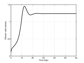
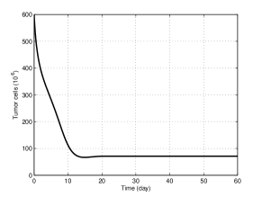
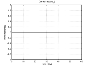
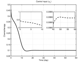
Figure 2: The effect of chemotherapy ($u_{1}$).

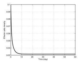
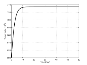
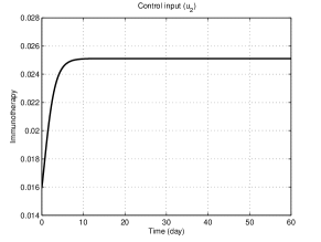
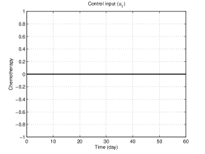
Figure 3: The effect of immunotherapy ($u_{2}$).

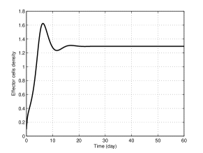
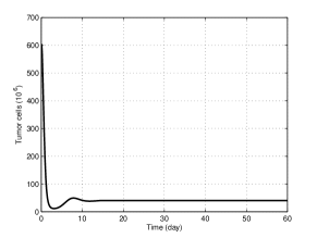
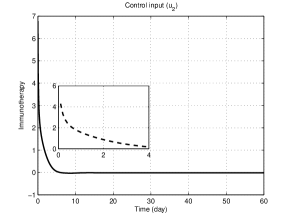
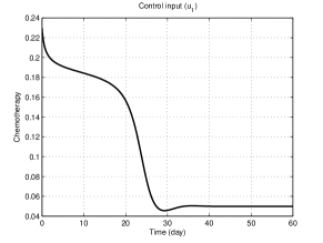
Figure 4: The effect of chemotherapy and immunotherapy.

Compared to the results of Ref. [24] that was accomplished on the same model used in this article, with the similar initial condition $X_{0}=\begin{bmatrix}600&0.1\end{bmatrix}^{T}$, it is seen that the designed controller in the current work is able to eliminate more tumor cells and also guarantees the positiveness of the closed-loop system in such a way that no positive constraints imposed to the variables. Additionally, the amplitude of the control inputs in this approach is lower than the one in [24]. In general, a maximum of 20 % of the full dose rate of the drug is approximately needed to control the progression of cancer. Accordingly, less control efforts are required for the cancer treatment and, consequently, the side effects of the treatment are reduced significantly. It should be noted that the maximum amount of cancer cells in the proposed method is much lower than the one in [24], which indicates a reduction in the likelihood of death during the course of treatment. In other words, by considering the initial condition $X_{0}=\begin{bmatrix}600&0.1\end{bmatrix}^{T}$ that belongs to the malignant status of the tumor, the proposed controller is an efficient tool for the goal of treatment.

5 Conclusion

This paper suggests a new fuzzy modeling approach for the nonlinear modified Stepanova’s model, which is one of the efficient and applicable models for the cancer treatment. In spite of the previous works that used optimal control strategies, this paper proposes a positive T–S fuzzy controller for the successful treatment of cancer under mixed immunotherapy and chemotherapy. This is based on a new framework that incorporates, for the first time, T–S fuzzy model, linear co-positive Lyapunov function, and parallel distributed compensation via a convex optimization approach. This new framework is a lot invaluable since there are inherent nonnegative sign features for the state variables and their corresponding control inputs. The simulation results show that the control structure can be successfully exploited to the tumor-immune system, which leads to the best performance in the sense that it significantly minimizes the volume of the tumor cells and, consequently, reduces the doses of the consumed drug. However, the population of the immune competent cells can reach an appropriate level, so that the immune system can prevent tumor growth. Future research will concern an extension of this method to the design of a controller considering uncertainties, disturbance, and unknown factors in the nonlinear model. The proposed methodology can also be applied in treating other specific types of cancer.

Appendix A A review on fuzzy systems and positive systems

In this section, brief reviews of T–S fuzzy systems and positive systems are provided. Moreover, several observations and results associated with the positive T–S fuzzy systems that are used throughout this paper are introduced. The T–S fuzzy system is one of the most widely used approaches for the stability analysis and controller design of nonlinear systems [15]. Explicitly, the T–S fuzzy model is described by fuzzy IF-THEN rules, where each locally characterizes linear input-output relations of the system through the sector nonlinearity technique.

Assume the $i$th plant rule of the T–S model is as follows:
Plant rule $i$: IF $\vartheta_{1}(k)\;is\;M_{i1}\;and,...,and\;\vartheta_{n}(k)\;is\;M_{in}\;$, THEN

$$\left\{\begin{array}[]{l}x(k+1)=A_{i}x(k)+B_{i}u(k),\\ z(k)=C_{i}x(k)+D_{i}u(k),\\ x(0)=x_{0}\succeq 0,\end{array}\right.$$ (29)

where $x(k)\in\mathbb{R}^{n}$, $u(k)\in\mathbb{R}^{m}$, and $z(k)\in\mathbb{R}^{l}$ are the state vector, input vector, and output vector, respectively. $i\in\mho_{r}=\{1,...,r\}$, $r$ is the number of IF-THEN rules. $\vartheta_{1}(k),...,\vartheta_{n}(k)$ and $M_{ij}$ are the premise variables and the membership functions, respectively. Then, the overall T–S model is given by:

$$S:\left\{\begin{array}[]{l}x(k+1)=\sum\limits_{i=1}^{r}h_{i}(\vartheta(k))(A_{i}x(k)+B_{i}u(k),\\ z(k)=\sum\limits_{i=1}^{r}h_{i}(\vartheta(k))(C_{i}x(k)+D_{i}u(k),\\ x(0)=x_{0}\succeq 0,\end{array}\right.$$ (33)

where

$$h_{i}(\vartheta(k))=\dfrac{\omega_{i}(\vartheta(k))}{\sum_{i=1}^{r}\omega_{i}(\vartheta(k))}, \qquad\omega_{i}(\vartheta(k))=\prod_{j=1}^{\mu}M_{ij}(\vartheta_{j}(k)),$$

$$\sum_{i=1}^{r}h_{i}(\vartheta(k))=1, \qquad 0\leq h_{i}(\vartheta(k))\leq 1,$$

and $M_{ij}(\vartheta_{j}(k))$ is the grade of membership of $\vartheta_{j}(k)$ in $M_{ij}$.

Here, the essential definitions and lemma are introduced.

Definition 1.

[17]: Given any positive initial condition $x(0)\geq\geq 0$ and input $u(k)\geq\geq 0$, the discrete-time system (33) is said to be positive if $x(k)\geq\geq 0$ and $z(k)\geq\geq 0$ for all integers $k\in R^{n}_{+}$.

Definition 2.

[17]: In the continuous-time system, a real matrix $A$ is called a Metzler matrix if its off-diagonal elements are positive, i.e. $A_{ij}\geq 0$, $i\neq j$.

Definition 3.

[17]: In the discrete-time system, a real matrix $\it A$ is called Schur if all its eigenvalues are strictly inside the unit circle.

Definition 4.

A linear map $V(x(k))=p^{T}x(k)$ with $V(0)=0$ is said to be an LCPLF for positive system $x(k+1)=Ax(k)$, if the following conditions hold for all $x\in\mathbb{R}^{n}_{+}$:

$$\begin{cases}V(x(k))>0,\\ \Delta V(x(k))<0.\end{cases}$$

Lemma 1.

[16]: The discrete-time T–S fuzzy system (33) is positive if and only if

$$A_{i}\geq\geq 0,\ B_{i}\geq\geq 0,\ C_{i}\geq\geq 0,\ D_{i}\geq\geq 0,$$

where $i=1,...,r.$

Remark 4.

When $x(0)\in R^{n}_{+}$ is not hold, $x(k)\geq\geq 0$, may not satisfy for all the sets of nonnegative integers even if all the conditions of Lemma (1) hold. In order to certify the advisable efficiency of Lemma (1), the satisfaction of $x(0)\in R^{n}_{+}$ is assumed.

References

- [1] C. H. Wang, J. K. Rockhill, M. Mrugala, D. L. Peacock, A. Lai, K. Jusenius, J. M. Wardlaw, T. Cloughesy, A. M. Spence, R. Rockne, et al., Prognostic significance of growth kinetics in newly diagnosed glioblastomas revealed by combining serial imaging with a novel biomathematical model, Cancer research (2009) 0008–5472.
- [2] S. Chareyron, M. Alamir, Model-free feedback design for a mixed cancer therapy, Biotechnology progress 25 (3) (2009) 690–700.
- [3] F. F. Teles, J. M. Lemos, Cancer therapy optimization based on multiple model adaptive control, Biomedical Signal Processing and Control 48 (2019) 255–264.
- [4] C. Cattani, A. Ciancio, Qualitative analysis of second-order models of tumor–immune system competition, Mathematical and Computer Modelling 47 (11-12) (2008) 1339–1355.
- [5] K. R. Fister, J. H. Donnelly, Immunotherapy: an optimal control theory approach., Mathematical biosciences and engineering: MBE 2 (3) (2005) 499–510.
- [6] N. Stepanova, Course of the immune reaction during the development of a malignant tumour, Biophysics 24 (5) (1979) 917–923.
- [7] A. d’Onofrio, U. Ledzewicz, H. Schättler, On the dynamics of tumor-immune system interactions and combined chemo-and immunotherapy, in: New challenges for cancer systems biomedicine, Springer, 2012, pp. 249–266.
- [8] A. M. A. Rocha, M. F. P. Costa, E. M. Fernandes, On a multiobjective optimal control of a tumor growth model with immune response and drug therapies, International Transactions in Operational Research 25 (1) (2018) 269–294.
- [9] M. C. Martins, A. M. A. Rocha, M. F. P. Costa, E. M. Fernandes, Comparing immune-tumor growth models with drug therapy using optimal control, in: AIP Conference Proceedings, Vol. 1738, AIP Publishing, 2016, p. 300005.
- [10] T. Chen, N. F. Kirkby, R. Jena, Optimal dosing of cancer chemotherapy using model predictive control and moving horizon state/parameter estimation, Computer methods and programs in biomedicine 108 (3) (2012) 973–983.
- [11] S. Chareyron, M. Alamir, Mixed immunotherapy and chemotherapy of tumors: feedback design and model updating schemes, Journal of theoretical biology 258 (3) (2009) 444–454.
- [12] D. Kirschner, J. C. Panetta, Modeling immunotherapy of the tumor–immune interaction, Journal of mathematical biology 37 (3) (1998) 235–252.
- [13] H. Nasiri, A. A. Kalat, Adaptive fuzzy back-stepping control of drug dosage regimen in cancer treatment, Biomedical Signal Processing and Control 42 (2018) 267–276.
- [14] T. Takagi, M. Sugeno, Fuzzy identification of systems and its applications to modeling and control, IEEE transactions on systems, man, and cybernetics (1) (1985) 116–132.
- [15] K. Tanaka, H. O. Wang, Fuzzy control systems design and analysis: a linear matrix inequality approach, John Wiley & Sons, 2004.
- [16] A. Benzaouia, A. Hajjaji, Advanced Takagi-Sugeno Fuzzy Systems, Springer, 2016.
- [17] L. Farina, S. Rinaldi, Positive linear systems: theory and applications, Vol. 50, John Wiley & Sons, 2011.
- [18] T. Kaczorek, Positive 1D and 2D systems, Springer Science & Business Media, 2012.
- [19] F. Cacace, L. Farina, R. Setola, A. Germani, Positive Systems: Theory and Applications (POSTA 2016) Rome, Italy, September 14-16, 2016, Vol. 471, Springer, 2017.
- [20] L. Norton, A gompertzian model of human breast cancer growth, Cancer research 48 (24 Part 1) (1988) 7067–7071.
- [21] A. Merola, C. Cosentino, F. Amato, An insight into tumor dormancy equilibrium via the analysis of its domain of attraction, Biomedical Signal Processing and Control 3 (3) (2008) 212–219.
- [22] F. Blanchini, P. Colaneri, M. E. Valcher, et al., Switched positive linear systems, Foundations and Trends® in Systems and Control 2 (2) (2015) 101–273.
- [23] A. Benzaouia, A. El Hajjaji, Conditions of stabilization of positive continuous Takagi–Sugeno fuzzy systems with delay, International Journal of Fuzzy Systems 20 (3) (2018) 750–758.
- [24] U. Ledzewicz, M. S. F. Mosalman, H. Schättler, Optimal controls for a mathematical model of tumor-immune interactions under targeted chemotherapy with immune boost, Discrete & Continuous Dynamical Systems-B 18 (4) (2013) 1031–1051.