Learning to Wait:
Wi-Fi Contention Control using Load-based Predictions

Abstract

We propose and experimentally evaluate a novel method that dynamically changes the contention window of access points based on system load to improve performance in a dense Wi-Fi deployment. A key feature is that no MAC protocol changes, nor client side modifications are needed to deploy the solution. We show that setting an optimal contention window can lead to throughput and latency improvements up to 155%, and 50%, respectively. Furthermore, we devise an online learning method that efficiently finds the optimal contention window with minimal training data, and yields an average improvement in throughput of 53-55% during congested periods for a real traffic-volume workload replay in a Wi-Fi test-bed.

1 Introduction

As more and more devices come on-line and demand an increasing amount of throughput and low latency [27], contention for the available wireless spectrum has become a growing problem [26].

Wi-Fi uses a Listen-Before-Talk (LBT) mechanism to access unlicensed spectrum in a fair and efficient way. The most used algorithm in today’s networks is the Binary-Exponential-Backoff (BEB) mechanism that forces transmitters to double their wait time after each failed transmission. Many researchers have shown in the past that this mechanism scales poorly as the number of interfering transmitters increases and that adjusting the contention window can improve performance [6, 8, 3].

The problem has been recently exacerbated by the trend in the latest Wi-Fi specifications [25, 20] to bond existing 20Mhz wide channels to 40, 80, and 160Mhz bands, in order to allow wireless end-user devices to take advantage of throughput increases in high-speed broadband backhauls [2].

Setting different QoS levels on different packets helps some high priority streams, but what if all streams are marked high priority? In other words, what if we want to improve the Wi-Fi experience without compromising fairness?

Many algorithms that improve BEB both in terms of throughput and fairness have been proposed [29, 31, 32, 14, 24], but failed to make an impact due to the inertia of (MAC) protocol adoption in Wi-Fi , in particular for end-user devices. Furthermore, a typical dense Wi-Fi deployment exhibits highly complex performance dynamics that are hard to reproduce in simulations alone. The complexity not only makes simulation results less reliable, but may also call for more flexible, and adaptable optimization models and methods.

In response to these challenges we have developed a novel machine-learning method to control the Wi-Fi contention window on access points (APs) deployed in a dense environment. Our method does not require any changes on client devices, or to the Wi-Fi protocols, while still being fair across both participating and exogenous devices.

We evaluate our method experimentally using a test-bed with off-the-shelf APs and Wi-Fi stations and using a trace of traffic volumes recorded from a real broadband deployment.

Our work extends the existing body of work by taking both transmitters and system load into account to predict the optimal wait times at any given time, and using a trained model capable of capturing correlations between easily observed measurements and optimal contention windows.

The key contribution is threefold:

• we propose a model to predict optimal contention windows (Section 3),

• we explore and quantify the opportunity of setting an optimal contention window experimentally in a test-bed (Section 6), and

• we propose a learning algorithm to continuously train our predictive model to adjust the contention window based on system load (Section 7)

The rest of the paper is organized as follows. We introduce the fundamentals of the Wi-Fi backoff mechanism in Section 2. Then we present our predictor models in 3, and the dataset used to replay traffic into our test-bed (Section 4), which in turn is described in Section 5. In Section 6 we run a series of experiments to showcase the opportunity in improving the contention mechanism implemented in current networks (BEB). Section 7 then shows the results of training and applying a predictive model for contention window control. In Section 8 we describe the architectural components of our implementation. We discuss related work in Section 9, and finally we conclude in Section 10.

2 Background

Shared medium access in Wi-Fi is implemented by the distributed coordination function (DCF) in the medium access control (MAC) layer. It is a contention-based protocol based on the more general carrier sense multiple access with collision-avoidance (CSMA/CA) protocol. When a frame is to be transmitted, a Listen-Before-Talk (LBT) mechanism is employed where the channel is first sensed and if busy the transmission attempt is delayed for a backoff period. The backoff period is determined by picking a uniformly random number of wait time slots, say $r$, in the interval $[0..CW]$, where $CW$ is the contention window. The starting point $CW$ is referred to as $CW_{min}$. The new transmission attempt is then made after $r$ time slots. Each slot is a standardized time interval, typically about $9\mu s$. The most commonly used backoff algorithm, binary exponential backoff (BEB), doubles the contention window, $CW$, for every failed attempt, up to a maximum value of $CW_{max}$. After a given number of failed attempts the frame is dropped, and the error is propagated to higher-level protocols or the application. In case of a successful transmission the contention window is reset to $CW_{min}$.

The enhanced distributed channel access (EDCA) amendment (802.11e) [22] introduced a QoS extension to DCF  for contention-based access. A number of parameters can be configured in different service classes, or transmission queues to give different priorities to different flows. One set of these parameters is the $(CW_{min},CW_{max})$ tuple. The standard specifies default values for this tuple, but access point administrators may change these values at will. For best effort (BE) traffic the default values are $(15,63)$ . Our approach is based on changing these parameters dynamically and always setting $(CW_{min},CW_{max})$ to $(CW_{opt},CW_{opt})$, to effectively disable the exponential backoff, and leave it fully in our control how long the transmitters have to wait on average before attempting to retransmit ($9CW_{opt}/2\mu s$ ).

Now the problem is reduced to finding and setting the optimal contention window, $CW_{opt}$ that maximizes some QoS parameter, such as throughput or latency. Here, we consider only single-step prediction of $CW_{opt}$. That is, we observe some state of the system in period $t_{0}$ and then set the contention window to use in period $t_{1}$. The motivation behind this setup is that predictions further into the future will be less accurate. Furthermore, if there is a long gap between observation and enforcement, and between enforcements, the true $CW_{opt}$ may change within allocation periods, leading to suboptimal allocations.

Note, that this rules out machine learning techniques such as reinforcement learning (RL), where allocation decisions in the current period is assumed to impact rewards in multiple future periods. In other words, the greedy optimization strategy is always optimal in our case. However, as we will discuss later, our approach is inspired by and borrows some techniques from RL.

3 Model

In [29] an adaptive backoff algorithm (ABA) is derived from the probability of collisions, given a fixed number of active transmitters, and a configured minimum CW, $CW_{MIN}$. The optimal CW is then estimated as follows:

$$CW_{opt}=\frac{CW_{MIN}}{2}\times a-1$$ (1)

where $CW_{MIN}$ is the default EDCA minimum contention window for the service class (15 for best effort), and $a$ the number of active transmitters .

We propose a generalization of the ABA model as follows:

$$log(CW_{opt})=\theta_{0}+\theta_{1}a+\theta_{2}{t\!p}$$ (2)

where the $\theta$ comprise the model coefficients to be trained, $a$ the observed number of active APs, and $t\!p$ the observed aggregate throughput from the last period.

Apart from the generalization and the additional load term, the model allows for continuous adaptation of the coefficients to fit the observed data. We will discuss a learning method that trains this model online in Section 7.

The load term was introduced to account for environment interference impacting the throughput, i.e. factors beyond the APs that we control.

Given the intended use for training with Machine-Learning methods, we call this general model (Equation 2) the Machine-Learning Backoff Algorithm (MLBA) model.

The log transform, which implies that the predictors are multiplicative as opposed to additive, is motivated by experiments in Section 7. Intuitively, the expected throughput of a transmitter at any given time is inversely proportional to the current contention window, and is also proportional to the product of the probabilities that other transmitters will not transmit at that time (see Appendix A.2).

3.1 Model Training

3.1.1 MLBA-LR

The simplest way to estimate the coefficients for an observed set of $\{a,{t\!p}\}$ input parameters (predictors) and optimal CW (response) is by Least squares regression, e.g. ordinary least squares (OLS), where a coefficient is estimated by the covariance of the parameter with the response variable (output). So to estimate $\theta$ above we compute:

$$\hat{\theta}_{0} =log(CW_{opt})-\hat{\theta}_{1}a-\hat{\theta}_{2}{t\!p}$$

$$\hat{\theta}_{1} =\frac{Cov[a,log(CW_{opt})]}{Var[a]}$$

$$\hat{\theta}_{2} =\frac{Cov[{t\!p},log(CW_{opt})]}{Var[{t\!p}]}$$

We call the backoff algorithm deploying this form of parameter estimation MLBA-LR.

3.1.2 MLBA-NB

Another approach is to learn model parameters through a Naive-Bayes method, where the contention window that maximizes the conditional probability of a given state $s=\{a,{t\!p\}}$ is chosen. The probability can be computed according to Bayes theorem as:

$$CW_{opt}=\operatorname*{arg\,min}_{CW}\left\{P(CW|s)\triangleq\frac{P(s|CW)\times P(CW)}{P(s)}\right\}$$ (3)

We call the backoff algorithm deploying this form of contention window estimation MLBA-NB.

3.1.3 MLBA-DNN

As a final model we propose a Deep Neural Network to estimate an optimal contention window $CW$ given a state $s$. A Deep Neural Network (DNN) is defined as having multiple hidden layers. Between every two layers is a (nonlinear) activation function that determines how to map output from one layer into inputs of the next layer. Our MLB-LR model can hence be seen as a collapsed single-layer DNN. Our minimal network configuration is, one input layer, two hidden layers, and one output layer. The output layer renders the final prediction and is thus often single-dimensional. The 3-layer (2 hidden layer) DNN model can then be expressed as:

$$CW_{o\!pt}(x)=\mathbf{b}^{(3)}+\mathbf{w}^{T}h(\mathbf{b}^{(2)}+\mathbf{W}^{(2)}h(\mathbf{b}^{(1)}+\mathbf{W}^{(1)}\mathbf{x}))$$ (4)

where $h()$ is the hidden layer activation function, in this case we use rectified linear units [12], $ReLu(x)=max(x,0)$, $\mathbf{x}$ is the input vector of $\{a,t\!p\}$ tuples, $\mathbf{W}^{(k)}$ is the matrix of weights for hidden layer $k$, $\mathbf{b}^{(k)}$ is the bias vector for layer $k$ ($k=3$ is the output layer) , and $\mathbf{w}$ is the vector of weights between the last hidden layer and the single cell output layer.

To train this model (using backpropagation) we apply mean-square-error as loss function , and the adam [21] stochastic gradient descent algorithm. We have flexibility in selecting the number of nodes in the hidden layers; more nodes would mean a more accurate fit but longer training time. It also depends on the variance of the number of transmitters and load. A high variance and complex interrelationships may require more nodes to model appropriately. We call the backoff algorithm deploying this form of contention window estimation MLBA-DNN.

Note here that a typical DNN is a supervised learning model, but as we shall see in Section 7, we create the training data on the fly and hence our method becomes unsupervised.

4 Traffic Volume Data

Given that the model we propose is predictive and should be capable of learning some hidden behavior in traffic volume dynamics, we collect a real-world trace from a residential deployment with cable modems connected to a cable headend (CMTS)  over a HFC  network. The data comprise download volumes on a per-second basis for each cable modem. Volumes were captured on July 1st 2017 from 8 cable modems.

Due to the fact that the rates are set dynamically in a Wi-Fi network based on the measured signal-to-interference-plus-noise ratio (SINR), we only capture whether the modem is active or not (the sum of active modems is quantity $a$ in Section 3), i.e. transmitting any data in each second of the trace, and we then let our test-bed (see Section 5) find the best rate.

The individual traces can be seen in Figure 1. We selected one hour for model building analysis, one hour for meta parameter evaluation and five hours for model prediction evaluation (see Section 7).

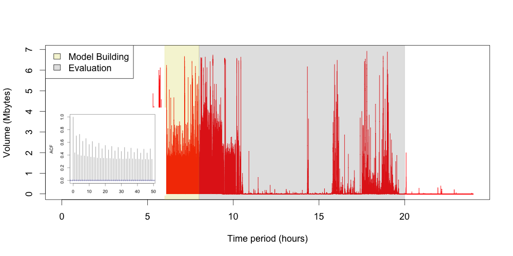
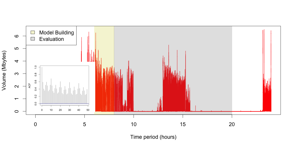
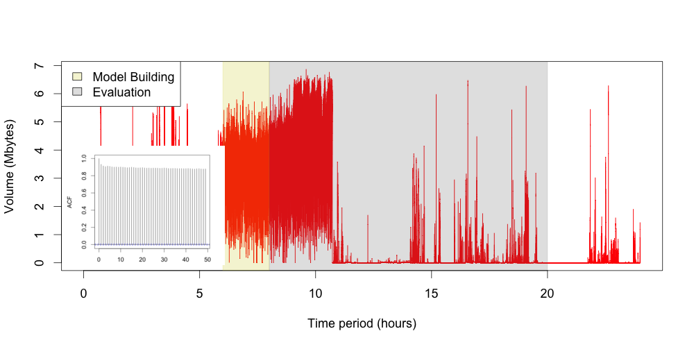
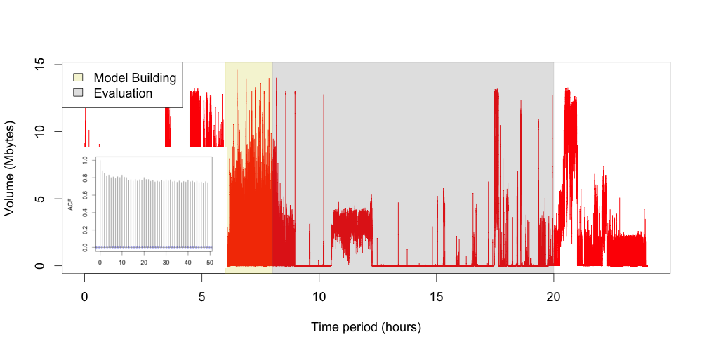
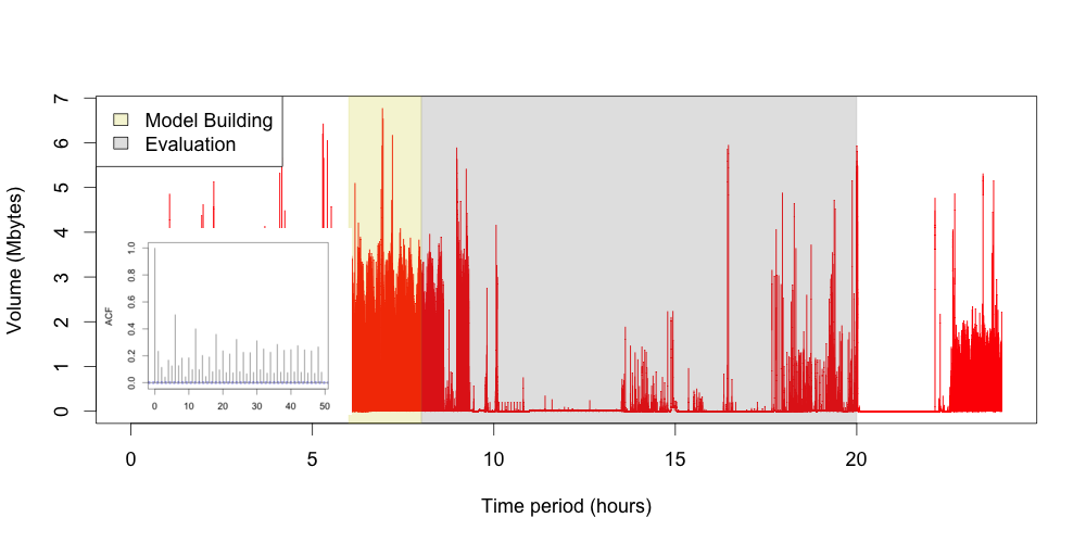
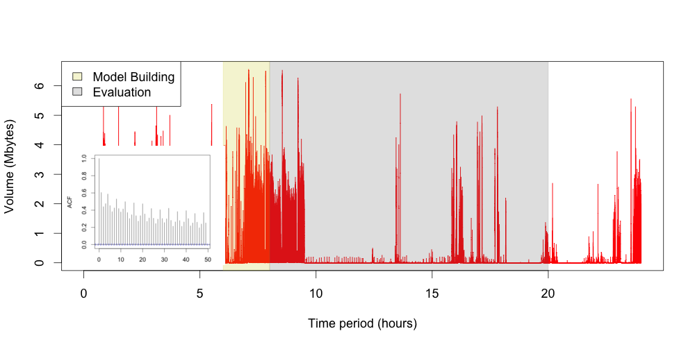
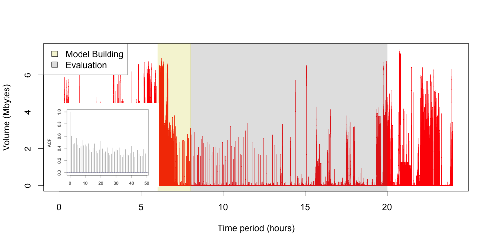
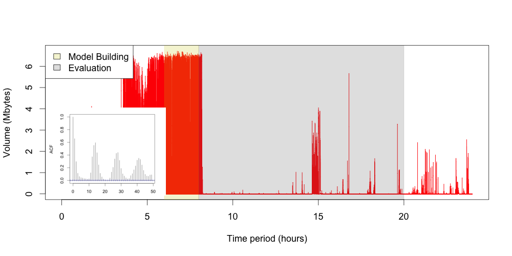
Figure 1: Workloads with ACF insets (seconds) from 8 cable modems

5 Testbed

Our test-bed comprises 8 Wi-Fi Access Points transmitting on the U-NII-3 80Mhz band. Two APs are TP-Link Archer AC1750 routers, and 6 are GLi GL-AR750S-Ext devices. All run the latest OpenWrt release with a patch we developed to control $CW_{min}$ and $CW_{max}$ from the hostapd control interface and CLI (see more details in Section 8).

We use an additional 8 GLi GL-AR750S-Ext as Wi-Fi clients, and 8 Raspberry Pi Model 3B to run iperf3 servers that the clients connect to. The iperf servers could also run on the APs but it leads to CPU contention, limiting the throughput instead of airtime, at higher rates.

All transmissions are done with 802.11ac VHT and a theoretical max throughput rate of 433Mbps. With iperf3 servers running on the APs the max throughput is around 100Mbps, whereas separating out the servers on the Pis improved the throughput to about 300Mbps.

All traffic is going in the direction from the AP to the clients, with unrestricted  TCP flows.

The distance between the APs and the clients vary between 5 and 10 feet, and the distance between the APs vary between 2 and 6 feet. Finally, the distance between the clients vary between 2 to 5 feet. Both clients and APs are stationary throughout all experiments.

A room layout sketch of the physical setup is shown in Figure 2.

All APs and clients are connected to an Ethernet switch to avoid control and measurement traffic interfering with the Wi-Fi link. The Raspberry Pis are also connected to their dedicated AP with a direct Ethernet cable connection.

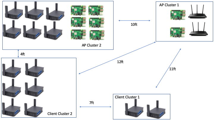
Figure 2: Test-bed layout sketch (not to scale). Note icon pictures show devices used, and AP cluster 2 uses the same device as the clients (GLi).

6 Opportunity Evaluation

The purpose of this section is to quantify what the improvements are assuming we set an optimal contention window.

We run experiments in our test-bed (see Figure 2), where we vary the number of APs transmitting data as well as the contention window used. We also vary the number of APs we control in the system. The ones we do not control are assumed to follow the default back-off mechanism (BEB) as well as use the default (EDCA) transmission queue settings.

We measure both the throughput and the latency across all the APs as well as across APs that we do not control.

We vary the number of APs transmitting between 2 and 8 and the $[cwmin,cwmax]$ between $[1,1]$ and $[1023,1023]$, and compare this to the default best effort contention window setting of $[15,63]$ as well as a best effort contention window setting of $[1,1023]$.

The dotted lines in all graphs represent the corresponding value for the default contention window with exponential backoff (BEB), i.e. for best effort $[cwmin,cwmax]=[15,63]$ unless otherwise stated.

6.1 Throughput Improvement

What is the improvement in throughput when setting an optimal contention window? From Figure 3 we see that the median throughput improvement goes up to 155% with 8 concurrent transmitters when selecting the optimal CW compared to using the default backoff mechanism.

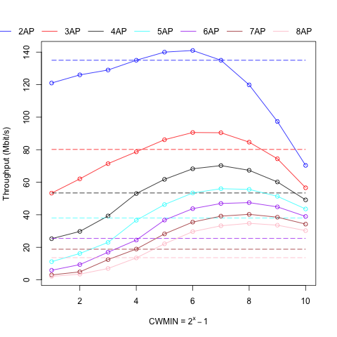
Figure 3: Median Throughput with different Contention Windows (CW) and transmitting APs.

6.2 Latency Improvement

What is the improvement in latency when setting an optimal contention window? We run the same experiments as above but now study the optimal latency in general as well as under the optimal throughput settings as measured above.

From Figure 4 we see that the median latency improvement goes up to 50% with 8 concurrent transmitters when selecting the optimal CW compared to using the default backoff mechanism. We also notice that the minimum latency point tends to coincide with the maximum throughput point (true for 3-8 APs, and close for 2 APs).

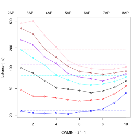
Figure 4: Median Latency with different Contention Windows (CW) and transmitting APs.

6.3 Partially Managed System

Can we improve throughput and latency even for streams we do not control? We ran the same experiment as above but we only control 4 of the 8 APs . The APs we do not control use the default backoff settings and mechanism.

Figure 5 shows that the aggregate throughput and latency still improves when we only control half of the APs.

Figure 6 shows that both the throughput and the latency improves for the APs we do not control. The way to read it is to first look at the optimal CW value in Figure 5 for 5, 6, 7 or 8 APs, and then compare the dotted line to the solid line value for that CW in this figure.

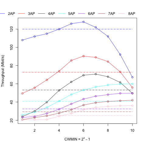
Figure 5: Overall Throughput and Latency with half of the APs controlled. X axis denotes CWs on APs we control.

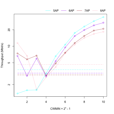
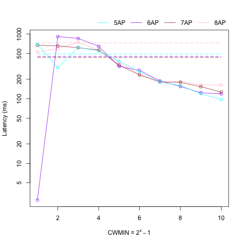
Figure 6: Throughput and Latency of APs not controlled. X axis denotes CWs on APs we control.

6.4 Window Range

If we let the contention window be adjusted with the default backoff mechanism (BEB), but change the minimum and maximum window to be the same as the minimum and maximum windows used by the dynamic method, does it improve or worsen the throughput and latency? 

Note, in the graphs in Figure 7, the dotted lines refer to $[cwmin,cwmax]=[1,1023]$. If we compare the dotted lines in Figure 3 and Figure 4 with the dotted lines in Figure 7, we can see that the extended range of the default backoff mechanism has a negative effect both on the throughput and on the latency. This shows that the default mechanism is not good at adjusting to the optimal window. Recall, that the default range for BEB best effort traffic, which is used here, is $[cwmin,cwmax]=[15,63]$.

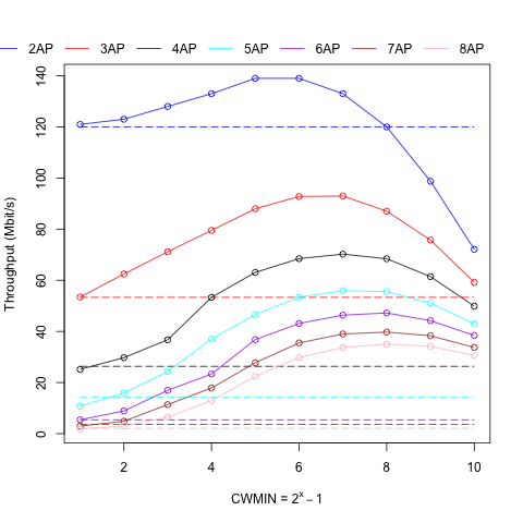
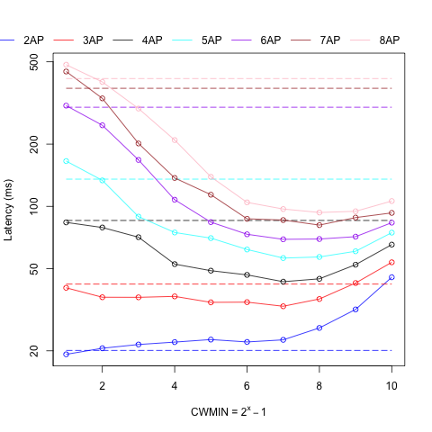
Figure 7: Throughput and Latency with default cwmin/max [1,1023]

6.5 Collision Reduction with Optimal Contention Window

What is the reduction in collisions if an optimal CW is used? We collect all the packets sent from 8 concurrent unlimited TCP streams both in the case of the default back-off mechanism and with the optimal CW for 8 transmitters in a saturated state. We then look at the 802.11 header Frame Control Field retry bit (12th frame control bit) and count the proportion of packets that were marked as retries. All packet captures cover 30 seconds (three 10 second bursts). With an optimal CW the system had $12$% retries or collisions, whereas the system with the default mechanism had $61$%, which is a $78$% reduction in collisions (retries). The total packet volume transmitted was $407$ MBytes with an optimal CW and $376$ MBytes with default.

6.6 RTS/CTS Impact

Does enabling RTS/CTS impact the collision probability? In all the experiments up to this point we have enabled RTS/CTS. Now, with an optimal CW and RTS/CTS turned off the collision probability measured as per above was $7$%, and with the default back-off and no RTS/CTS the probability of a collision was $33$%. Hence, in an RTS/CTS scenario the reduction in collisions was $78$%. So although there are fewer collisions overall the proportional reduction is the same. These results are summarized in Table 1. The total packet volume transmitted was $406$ MBytes with an optimal CW and $383$ MBytes with default. The collision probability drops by half, and the optimal CW also drops slightly, when RTS/CTS is disabled. More drastically, the throughput (goodput) improvement of setting an optimal CW goes down to about $13$% from about $155$% (see results in Section 6.1 for 8 APs). The change is solely due to the default backoff mechanism improving when RTS/CTS is turned off. The throughput numbers when using an optimal CW are roughly the same, when RTS/CTS is on and when it is off. However, RTS/CTS needs to be turned on in dense environments to avoid hidden node issues, and with sufficiently large number of competing transmitters it will likely start decaying again even without RTS/CTS. Note, that this result may seem counter-intuitive as RTS/CTS is often enabled to decrease collisions. But this experiment shows that there is a point of overload where the RTS/CTS frames themselves can cause too many collisions.

Table 1: Collision Probability (%)

	Default	Optimal
With RTS/CTS	$61$	$12$
No RTS/CTS	$33$	$7$

6.7 Fairness

Is it fairer to set both cwmin and cwmax to be the same optimal value across all APs than using an exponential backoff? To test this assertion we run the same benchmark with 8 concurrent transmitters (APs),$n=8$, using unlimited TCP traffic and measure the Jain Fairness Index [15]:

$$\frac{\left(\sum_{i=1}^{n}{x_{i}}\right)^{2}}{n\sum_{i=i}^{n}{x_{i}^{2}}}$$ (5)

where $x$ is the throughput and $n$ the number of transmitters. The value is between $\frac{1}{n}$, minimum fairness, and $1$, maximum fairness. In a sample of 5 runs, and when setting an optimal cw we get a Jain index of $0.982\pm 0.006$ and for the default backoff mechanism we get $0.980\pm 0.17$ with a $95$% confidence band assuming a normal distribution. The mean value difference is not significant, as both values are very high with 8 streams, but the variance in values is significantly larger with the default backoff algorithm. The conclusion is hence that setting the same optimal contention window across all APs is fair, as expected. We also note that the default $[cwmin,cwmax]$ range for best effort traffic is $[15,63]$ so the unfairness as a result of doubling the wait time is limited. If we instead set the $[cwmin,cwmax]$ to $[1,1023]$ we get a Jain index of $0.816\pm 0.059$ which is significantly lower and showcases the danger of exponential backoff. We also note that Heusse et.al. ran simulations producing similar results in [14] (Figure 1).

7 Model Evaluation

We now turn to workload-based experiments where we replay the data described in Section 4 in our test-bed. We first analyze the data to determine which type of models are appropriate, then we discuss our general method in some more detail, train model meta parameters, and simulate training speed. Finally we run an online test, benchmarking different models.

7.1 Model Analysis

First we investigate the relationship between aggregate load, active transmitters (APs) and optimal CW. For this purpose we replay 1 hour (3600 data points) of our 8 workloads concurrently (see Figure 1). For each data point replayed we measure the throughput obtained with different contention windows (1..1023). After the full replay is done we pick the optimal cw setting given observed throughput from the last period as well as observed number of active APs. We call this process, offline or exhaustive calibration.

We fit Equation 2 in Section 3 to the measurements and obtain an $R^{2}$ fit of $0.93$. The fitted model for this hour can be represented as:

$$log(CW_{opt})=-3.6+0.19a+2.7\times 10^{-8}tp$$ (6)

where $t\!p$ is in bits/s. All coefficients are statistically significant. The regression lines for different activity levels can be seen in Figure 8. We note that a model without log transform renders an $R^{2}$ of $0.73$.

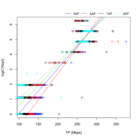
Figure 8: Offline model fit.

7.2 Method

Of course the exhaustive calibration we used above cannot be applied in a real system where you only get to see each load condition once and only get to pick one contention window to test. Even if an approximate exhaustive calibration could be performed, we want to minimize the training required to fit the parameters and also ensure that the parameters evolve over time to fit new behavior in the load conditions. For example a new source of interference introduced could simply be encoded as a new multiplier in the actives (number of active transmitters) parameter coefficient.

We now describe how to train the models described in Section 3, i.e. how to find and update the coefficients in Equation 2 online. Training of the model proceeds in the following three steps:

1. Create a CW Observation List (CWObs Queue)

2. Update a Table recording optimal CWs (CWMax Table)

3. Fit Regression Model

The CWObs Queue is comprised of two FIFO sub-queues of observed 4-tuples. One for calibration data and one for predicted values. The 4-tuples include: last observed aggregate throughput (tplast), last observed active transmitters (actives), cw enforced (cwenf), and throughput obtained with enforced cw (tp). An example fictive CWObs List can be seen in Table 2.

Table 2: Example CWObs Queue

tplast	actives	cwenf	tp
$123489331$	$20$	$15$	$223489331$
$223489331$	$22$	$31$	$323489331$

The two FIFO sub-queues are needed since calibration involves cycling through all possible CW values, and if these calibration points disappear the algorithm may be locked into a suboptimal region, if it were solely based on predictions.

The CWMax Table is updated whenever there is new data in the CWObs Queue. The table quantizes actives into alevel and tplast into tlevel levels and records the optimal cw cwopt used for the maximum tp as mtp at that level. An example fictive CWMax table can be seen in Table 3.

Table 3: Example CWMax Table

alevel	tlevel	mtp	cwopt
$1$	$1$	$123489331$	$15$
$1$	$2$	$223489331$	$31$

Finally, we fit a ML regression model (see Section 3.1) as per Equations 2, 3, and 4 with {alevel,tlevel} tuples from the table as features and cwopt as targets. Note mtp is only kept in the table to be able to update cwopt.

Now, the model execution (prediction) part of the algorithm can proceed as follows:

1. Map the observed actives and throughput to the corresponding {alevel,tlevel}-level tuple

2. Use the trained model to predict the cwopt with this level as input, and set it on all APs

3. Track the cw used and record the throughput obtained in the next time period, and add it to the CWObs Queue

Note that thanks to the CWobs queue the quantization of levels can be done dynamically based on the current content in the queue, to avoid sparsity in the CWMax Table. We also need to ensure that the queue has a wide set of cwenf values, so some initial or random exploration at infrequent intervals need to be performed to avoid lock-in into a cw range.

We also note that the approach assumes that there is a good correlation between the number of active transmitters, and the aggregate load from one period to the next. In other words we assume the process has the Markov property. We have verified (see the ACF charts in Figure 1) that this is true for our traces in periods from 1 to 10s. If this were not true we would not feed the observed actives and load levels into our models, but the predicted values . We have used some ML models for this task too but it is overkill with the tested data sets due to the high autocorrelations. For more complex models with hidden parameters like DNN it could also capture the predictive aspect of these values, but that remains to be verified.

7.3 Calibration Period Estimation

To determine how much training data is needed for our predictions to reach the optimal performance, and to get a sense for how frequently the models need to be recalibrated, we ran training simulations using the data generated by the offline calibration. Recall, that the offline training data contains a record for each step in the workload trace for each possible contention window, recording the throughput obtained.

Simulating a real run thus involves picking a single record corresponding to a single contention window for each step. We compare BEB, ABA and MLBA vs an optimal picker that always picks the contention window with the optimal throughput value. For MLBA we use Linear Regression (LR), Deep Neural Network (DNN) and Naive Bayes (NB) for parameter estimation.

During a training phase we pick random contention windows before we train our model with the recorded data and start making predictions. Now we vary the steps, recall each step is a second, used before we start predictions. The predictions are then used throughout the data set which is one hour, or 3600 data points.

The throughput obtained compared to the optimal throughput for BEB, ABA and MLBA are shown in Figure 9.

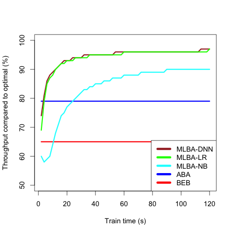
Figure 9: Prediction performance with different train times.

We note that we reach the performance of ABA with MLB almost instantaneously with just a few data points in our trained model. The prediction performance then converges to its best result at about 95% of optimal after about 35 seconds. MLBA-DNN performs marginally better than MLBA-LR and tends to reach plateaus earlier. MLBA-NB converges very slowly compared to the other MLBA algorithms. The DNN model is configured with 10 nodes in both hidden layers.

Based on this result we set our calibration period (where we round robin CWs) to 30 seconds.

7.4 Training History Estimation

Now, how much data should we keep in our CWobs and CWmax tables before we evict old values? And how often should we recalibrate and explore new CW values that are not predicted to be optimal? To answer those questions we pick a 15 minute period (900 data points) and run all our training algorithms with different parameter values for table size and re-calibration probability . Table 4 shows the results. History denotes the size of the CWobs table and calib. denotes the probability of exploring and calibrating new CW values. The table also shows the median throughput improvement over BEB for the different algorithms.

Table 4: Training History and re-calibration frequency summary

history	calib. (%)	LR (%)	NB (%)	DNN (%)
$150$	$1$	$50.8$	$54.3$	$52.9$
$\mathbf{600}$	$\mathbf{1}$	$\mathbf{52.5}$	$\mathbf{54.1}$	$\mathbf{55.3}$
$300$	$1$	$54.1$	$49.5$	$56.6$
$300$	$5$	$52.7$	$56.0$	$51.4$
$300$	$10$	$50.3$	$43.9$	$51.1$

The configuration with the overall best improvements across all training algorithms was a history of 600 seconds and re-calibration frequency 1% . Hence, we pick that configuration for the subsequent benchmarks. We also note that DNN outperformed LR in 4 of 5 tests, and NB in 3 of 5 tests. DNN also achieved the overall highest improvement, $56.6\%$.

7.5 Longitudinal Benchmarks

Finally, using the best performing configuration described above, we test our backoff method across five 15 minute-periods succeeding the model building period, see Figure 1, and compare the throughput between BEB, ABA, and the MLBA algorithms. To cover a larger time span, we only test the first 15 minutes of each of the 5 hours in the test set.

The results can be seen in Figure 10.

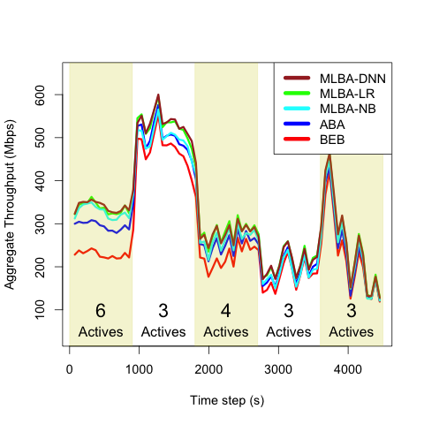
Figure 10: Prediction test results (1-minute averages) for 5 test periods and with average actives for each period displayed.

We group actives into two levels (${0..3}$ and ${4..8}$, $alevel=1$ and $alevel=2$) and use 5 load levels ($tlevel=[0,5)$) based on measured percentiles to reduce the sparsity of the throughput list data.

To test significance of differences between methods we take the empirical percentile of percent difference between the methods, period-by-period. We then measure the average difference and the percentile where the method tested starts getting a positive difference. For example, if method A on average across all replayed time steps (seconds) achieves an aggregate throughout across all APs that is 35% higher than method B and method A has a higher throughput than B in 70% of all time steps we say: $Avg(A>B)=35$ and $SigL(A>B)=30$. $SigL$ here can be compared to a one-tailed statistical significance level, in that a 5% significance level  is equivalent to $SigL(A>B)=5$. Table 5 summarizes the statistical test results.

Table 5: Average Improvements and Significance Levels. The five time-period results (see Figure 10) are parenthesized.

Hypothesis	Avg (%)	SigL (%)
ABA > BEB	$13(31,8,14,7,5)$	$15(\mathbf{5},20,10,20,30)$
LR > BEB	$\mathbf{25}(49,16,27,17,14)$	$\mathbf{10}(\mathbf{5},10,10,15,20)$
DNN > BEB	$\mathbf{26}(53,18,26,16,14)$	$\mathbf{10}(\mathbf{5},10,10,15,20)$
NB > BEB	$18(48,10,19,5,8)$	$20(\mathbf{5},20,15,40,30)$
LR > ABA	$10(15,8,12,9,9)$	$15(\mathbf{5},20,15,20,20)$
DNN > ABA	$11(17,10,11,9,9)$	$15(\mathbf{5},20,15,20,25)$
NB > ABA	$4(13,2,5,-2,3)$	$40(10,50,40,65,45)$
DNN > LR	$1(3,2,0,-1,0)$	$50(35,40,55,60,55)$
DNN > NB	$7(4,9,7,11,6)$	$25(30,20,25,20,20)$

We note that our MLBA algorithms do better in periods of more heavy load (e.g. period 1 in Table 5) compared to both ABA and BEB, and those are also the periods where MLBA-DNN tends to do slightly better than MLBA-LR.

8 Implementation

We have implemented a patch for hostapd in the latest OpenWrt release (18.06.1) that exposes the $CW_{min}$ and $CW_{max}$ settings for the transmission queues. It allows us to control all queues, although our experiments only change the best effort (BE) queue setting. The patch uses the hostapd control interface and also adds new hostapd_cli commands.

Depending on the deployment scenario we offer two ways to control the APs. The LAN controller is appropriate if the controller can be deployed in the local network, and the Cloud Controller is approprate if the APs only only had outbound access and should be controlled from an external network, e.g. a Cloud platform.

8.1 LAN Controller

In the LAN controller setup we provide a HTTP REST API exposed from the APs directly. Hostapd_cli is used behind a lighttpd Web server via CGI. The CGI scripts are then invoked by an HTTP client remotely from the controller. The roundtrip time to either call our custom CW control APIs or the pre-existing all_sta call to collect transmission data is about 20ms, without any optimizations. To improve the performance further a custom TCP sever embedding the hostapd_cli protocol could be used on the AP. The advantage of the current solution is, however, that it requires minimal modifications on the AP and leverages existing standard applications already in use in most APs today.

After collecting data with this interface, the controller feeds it into our contention window predictor, which then uses the load data to estimate active transmitters, and load, and finally predict the optimal CW. The optimal CW is then set across all APs using the same interface.

Collecting data, and making prediction is all done online and continuously in windows of 1 to 10s.

The controller and predictor are both written in Python using numpy, sklearn, keras, tensorflow, and scipy, and also comprises a http client that converts the hostapd control interface output into JSON. The controller also exposes a Flask-based REST interface for monitoring the status of the system and predictions.

The LAN controller architecture is depicted in Figure 11.

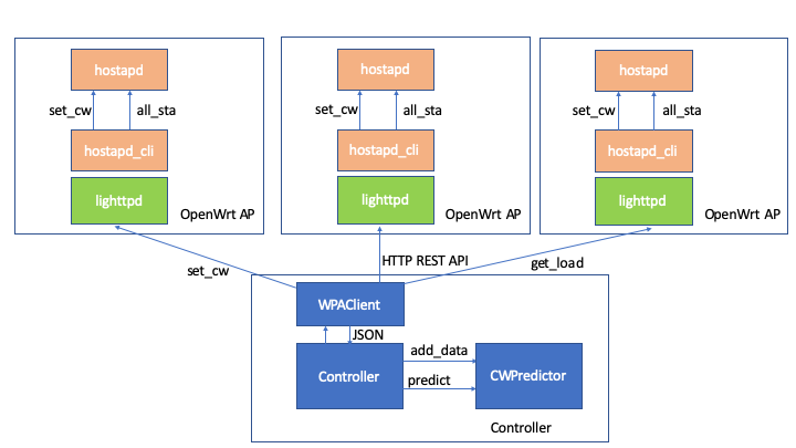
Figure 11: LAN Controller Contention Window Control Software Architecture.

All the experiments presented in this paper use the LAN controller API.

8.2 Cloud Controller

If the controller that is responsible for changing the contention window and collecting load from the APs is deployed in a network that does not have inbound access to the network where the APs are deployed, which is typical for Cloud deployments, we also provide a pubsub API that effectively turns pushes into pulls and allows similar control as if the AP API could be accessed directly. Instead of using the lighttpd server API this model make use of a lua socket client that long-polls a python Flask server on the remote network. This server in turn has an API that allows direct access to set the contention window and request load. When load is requested the APs push the current values to a Load cache in the cloud, implemented using Redis. The controller can then obtain the payload for all APs directly from Redis. Before flushing the load (only most recent values are kept in memory), the load data is written to a database for off-line analysis. The database is implemented in InfluxDB. The collection and prediction interval can, like the LAN controller, be set to between 1 to 10s, note however that this architecture increases the latency both to set the contention window and to collect load, but what is lost in latency is gained in scalability as all the APs are independently polling the PubSub channel and executing load and cw change commands. Hence this solution is also recommended for larger deployments. Finally, we also note that the AP to Controller communication goes across networks and potentially over the Internet, in the cloud deployment case, so the protocol runs over HTTPS using the OpenWrt luasec package.

The Cloud controller architecture is depicted in Figure 12.

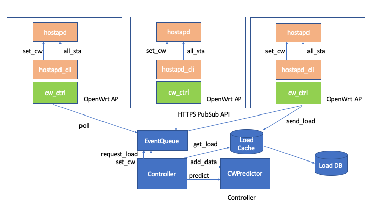
Figure 12: Cloud Controller Contention Window Control Software Architecture.

An internal pilot that we currently run with 10 APs is using this architecture.

9 Related Work

Contention window control: Load and active-transmitter based adjustment of CW using control theory or theoretically motivated equations have been studied in [29, 31, 32, 14, 24, 6]. In addition to applying machine-learning algorithms to capture both active transmitter and load correlations dynamically, and focussing on AP control, we also differ from these studies in our focus on test-bed evaluations with off-the-shelf hardware, and AP control.

Dense Wi-Fi optimization:  [5, 23, 18, 10] propose different load balancing techniques to improve the Wi-Fi QoE dynamically and deal with interference in dense environments. Our approach differs from this work in that the control is completely transparent to clients and no new connections have to be re-established as part of combatting load issues. Wi-Fi 6 [11] offers BSS coloring for spatial reuse, but only for Wi-Fi 6 clients, and it is based on signal detection thresholds as opposed to contention window tuning, and is thus orthogonal and complimentary to our approach.

Machine-Learning based network management: In  [17, 16, 19, 33, 1, 34] various DNN and Q-Learning approaches are proposed to optimize network configuration. We opted to use a custom Q-table like structure to train our models and then use an additional step of model fitting, to allow us to easily test and tune different fitting and online training models separately. Furthermore, we could not find a good intuitive way to explain why a lower immediate-reward CW could be picked in the current period just because of a potential future higher reward with another CW, and hence we use single-period predictions.

Cognitive Radio control: A Cognitive Radio Network (CRN) [13] shares our goal of improving the efficiency of a shared spectrum by sensing the environment. The typical goal of a cognitive radio is to determine whether a primary user (PU) is active on a frequency band, and if not allow secondary users (SU) to use it. Some approaches take energy sensing data from multiple radios to make a centralized decision [30, 35]. Machine learning techniques lend themselves well to this problem [7], in particular various classification techniques such as support vector machines (SVM), k-means clustering, and kernel-based learning have shown good results [4, 9]. Our approach does not require changing the frequency on any radios, and is thus fully transparent to the receivers, and only require a minimal software patch on the transmitters.

10 Conclusion

In this paper we have shown experimentally that there is a great opportunity to improve upon the Wi-Fi EDCA contention window backoff algorithms, using a predictive model trained with machine learning.

We note that the predictive model is trained for a saturated system. A non-saturated system does not have the same contention issues, in that the default BEB algorithm works better under those conditions. Hence, a separate learner could be applied to predict whether the system will be saturated in the next time period, if that is not the case use the default BEB algorithm.

As a final note, given that we take signals of actual throughput achieved by the APs we control into account, interfering APs could to some degree be indirectly accounted for without having to monitor them directly. The full impact of that is hard to estimate without field trials though, which is our next step.

Future work also includes deploying sensors to accommodate more direct load estimates from exogenous networks, i.e. other Wi-Fi or unlicensed band LTE (e.g. LAA) traffic not being controlled in the prediction of optimal contention window.

Appendix A Appendix

A.1 Known results for proportional fair
sharing

Consider $N$ stations, where the transmission probability of station $i$ is denoted $p_{i}$, $i=1,\dots,N$. Denote the throughput for station $i$ by $x_{i}$, $i=1,\dots,N$. For proportional fairness, we require the optimal transmission probabilities $p_{i}$ (and thereby the optimal minimum contention windows) to maximize $\sum_{i=1}^{N}w_{i}\log x_{i}$, where $w_{i}$, $i=1,\dots,N$ are weights for the stations. In [28, Sec. 3.2.1] it is shown that if all stations have the same physical layer transmission rate, then the optimal minimum contention window $\text{CW}_{\min,i}$ of station $i$ to be inversely proportional to the expected throughput $\text{E}[X_{i}]$ of station $i$:

$$\frac{1}{\text{CW}_{\min,i}}\propto\text{E}[X_{i}],\quad i=1,\dots,N.$$ (7)

Further, the expected throughput is given by [28, Sec. 3.1]:

$$\text{E}[X_{i}]\propto p_{i}\prod_{\begin{subarray}{c}j=1\\ j\neq i\end{subarray}}^{N}(1-p_{j}),\quad i=1,\dots,N,$$ (8)

with the transmission probabilities given by

$$p_{i} \approx\frac{2}{\text{CW}_{\min,i}+1}$$

$$\propto\frac{1}{\text{CW}_{\min,i}},\quad i=1,\dots,N,$$ (9)

and

$$\text{E}[\text{CW}_{i}]\approx\text{CW}_{\min,i},\quad i=1,\dots,N.$$ (10)

A.2 Heuristics derived from known results

To derive the heuristic relationship between $\log\,\text{CW}_{\min}$ and $a$, the number of active stations, and $\sum_{j=1}^{N}x_{j}$, the throughput, we first assume that $p_{i}=p$, $i=1,\dots,N$, and $X_{1},\dots,X_{N}$ are independent and identically distributed (i.i.d.). Note that this also implies that $\text{CW}_{\min,i}=\text{CW}_{\min}$, $i=1,\dots,N$. Assuming $p$ small and $N$ large, we have

$$\frac{1}{\text{CW}_{\min,i}} \propto\text{E}[X_{i}]$$

$$\propto p_{i}\prod_{\begin{subarray}{c}j=1\\ j\neq i\end{subarray}}^{N}(1-p_{j})$$

$$\approx p\exp[-(N-1)p]$$

$$\approx p\exp(-Np)$$

$$\approx\frac{2}{\text{E}[\text{CW}_{\min,i}]+1}\exp(-Np)$$

$$\propto\exp(-Np).$$ (11)

A.2.1 Heuristic relationship between $\log\,\text{CW}_{\min}$ and $a$

Note that $Np$ is the mean number of active stations, i.e., it is $\text{E}[A]$, where $A$ is the random variable representing the number of active stations. If we focus on a sample size of one (in the transmission interval under consideration), we substitute the observed quantity $a$ for the mean $\text{E}[A]=Np$ in (11), thereby yielding

$$\frac{1}{\text{CW}_{\min,i}}\propto\exp(-a)\Leftrightarrow\log\,\text{CW}_{\min}\propto a.$$ (12)

A.2.2 Heuristic relationship between $\log\,\text{CW}_{\min}$ and $\sum_{j=1}^{N}x_{j}$

From the inverse relationship between $p$ and $\text{CW}_{\min}$ given by (9), and the inverse relationship between $\text{CW}_{\min}$ and $\text{E}[X_{i}]$ given by (7), we can rewrite $Np$ as follows:

$$Np \propto\frac{N}{\text{CW}_{\min}}$$

$$\propto N\,\text{E}[X_{i}]$$

$$=\text{E}\left[\sum_{j=1}^{N}X_{j}\right],$$ (13)

which when combined with (11) yields

$$\frac{1}{\text{CW}_{\min,i}}\propto\exp\left\{-\text{E}\left[\sum_{j=1}^{N}X_{j}\right]\right\}.$$ (14)

Again, focusing on a sample size of one (in the transmission interval under consideration), we substitute the observed quantity $\text{tp}\equiv\sum_{j=1}^{N}x_{j}$ for the mean $\text{E}[\sum_{j=1}^{N}X_{j}]$ in (14), thereby yielding

$$\frac{1}{\text{CW}_{\min,i}}\propto\exp\left(-\sum_{j=1}^{N}x_{j}\right)\Leftrightarrow\log\,\text{CW}_{\min}\propto\text{tp}.$$ (15)

References

- [1] Dario Bega, Marco Gramaglia, Marco Fiore, Albert Banchs, and Xavier Costa-Perez. Deepcog: Cognitive network management in sliced 5g networks with deep learning. In IEEE INFOCOM 2019-IEEE Conference on Computer Communications, pages 280–288. IEEE, 2019.
- [2] Richard Bennett, Luke A Stewart, and Robert Atkinson. The whole picture: Where america’s broadband networks really stand. The Information Technology & Innovation Foundation, February, 2013.
- [3] Giuseppe Bianchi. Performance analysis of the ieee 802.11 distributed coordination function. IEEE Journal on selected areas in communications, 18(3):535–547, 2000.
- [4] Mario Bkassiny, Yang Li, and Sudharman K Jayaweera. A survey on machine-learning techniques in cognitive radios. IEEE Communications Surveys & Tutorials, 15(3):1136–1159, 2012.
- [5] Ayon Chakraborty, Shruti Sanadhya, Samir R Das, Dongho Kim, and Kyu-Han Kim. Exbox: Experience management middlebox for wireless networks. In Proceedings of the 12th International on Conference on emerging Networking EXperiments and Technologies, pages 145–159. ACM, 2016.
- [6] Alparslan Cil, Mehmet Akar, and Emin Anarim. Adaptive optimization of edca parameters for improved qos in multi-media applications. Turkish Journal of Electrical Engineering & Computer Sciences, 20(Sup. 2):1369–1388, 2012.
- [7] Charles Clancy, Joe Hecker, Erich Stuntebeck, and Tim O’Shea. Applications of machine learning to cognitive radio networks. IEEE Wireless Communications, 14(4):47–52, 2007.
- [8] Der-Jiunn Deng, Shao-Yu Lien, Jorden Lee, and Kwang-Cheng Chen. On quality-of-service provisioning in ieee 802.11 ax wlans. IEEE Access, 4:6086–6104, 2016.
- [9] Guoru Ding, Qihui Wu, Yu-Dong Yao, Jinlong Wang, and Yingying Chen. Kernel-based learning for statistical signal processing in cognitive radio networks: Theoretical foundations, example applications, and future directions. IEEE Signal Processing Magazine, 30(4):126–136, 2013.
- [10] Edgewater Wireless. Building a better high density wifi solution starts here, 2018.
- [11] Matthew Gast. 802.11Ac: A Survival Guide. O’Reilly Media, Inc., 1st edition, 2013.
- [12] Richard HR Hahnloser, Rahul Sarpeshkar, Misha A Mahowald, Rodney J Douglas, and H Sebastian Seung. Digital selection and analogue amplification coexist in a cortex-inspired silicon circuit. Nature, 405(6789):947, 2000.
- [13] Simon Haykin. Cognitive radio: brain-empowered wireless communications. IEEE journal on selected areas in communications, 23(2):201–220, 2005.
- [14] Martin Heusse, Franck Rousseau, Romaric Guillier, and Andrzej Duda. Idle sense: an optimal access method for high throughput and fairness in rate diverse wireless lans. In ACM SIGCOMM Computer Communication Review, volume 35, pages 121–132. ACM, 2005.
- [15] Raj Jain, Arjan Durresi, and Gojko Babic. Throughput fairness index: An explanation. In ATM Forum contribution, volume 99, 1999.
- [16] Junchen Jiang, Vyas Sekar, Henry Milner, Davis Shepherd, Ion Stoica, and Hui Zhang. CFA: A practical prediction system for video qoe optimization. In 13th USENIX Symposium on Networked Systems Design and Implementation (NSDI 16), pages 137–150, 2016.
- [17] Junchen Jiang, Shijie Sun, Vyas Sekar, and Hui Zhang. Pytheas: Enabling data-driven quality of experience optimization using group-based exploration-exploitation. In 14th USENIX Symposium on Networked Systems Design and Implementation (NSDI 17), pages 393–406, 2017.
- [18] Ramanujan K Sheshadri, Mustafa Y Arslan, Karthikeyan Sundaresan, Sampath Rangarajan, and Dimitrios Koutsonikolas. Amorfi: Amorphous wifi networks for high-density deployments. In Proceedings of the 12th International on Conference on emerging Networking EXperiments and Technologies, pages 161–175. ACM, 2016.
- [19] Jiheon Kang and Doo-Seop Eom. Offloading and transmission strategies for iot edge devices and networks. Sensors, 19(4):835, 2019.
- [20] Evgeny Khorov, Anton Kiryanov, Andrey Lyakhov, and Giuseppe Bianchi. A tutorial on ieee 802.11 ax high efficiency wlans. IEEE Communications Surveys & Tutorials, 21(1):197–216, 2018.
- [21] Diederik P Kingma and Jimmy Ba. Adam: A method for stochastic optimization. arXiv preprint arXiv:1412.6980, 2014.
- [22] Stefan Mangold, Sunghyun Choi, Peter May, Ole Klein, Guido Hiertz, and Lothar Stibor. Ieee 802.11 e wireless lan for quality of service. In Proc. European Wireless, volume 2, pages 32–39, 2002.
- [23] Rohan Murty, Jitendra Padhye, Ranveer Chandra, Alec Wolman, and Brian Zill. Designing high performance enterprise wi-fi networks. In NSDI, volume 8, pages 73–88, 2008.
- [24] Paul Patras, Albert Banchs, Pablo Serrano, and Arturo Azcorra. A control-theoretic approach to distributed optimal configuration of 802.11 wlans. IEEE Transactions on Mobile Computing, 10(6):897–910, 2010.
- [25] Eldad Perahia and Robert Stacey. Next generation wireless LANs: 802.11 n and 802.11 ac. Cambridge university press, 2013.
- [26] Michael Philpott. The role of wi-fi in the premium home broadband marker. Ovum Report, 2016. Available at https://ovum.informa.com/resources/product-content/the-role-of-wi-fi-in-the-premium-home-broadband-market.
- [27] Sandvine. Global internet phenomena report. Sandvine Report, 2016. Available at https://www.sandvine.com/trends/global-internetphenomena/.
- [28] Vasilios A Siris and George Stamatakis. Optimal cwmin selection for achieving proportional fairness in multi-rate 802.11 e wlans: test-bed implementation and evaluation. In Proceedings of the 1st international workshop on Wireless network testbeds, experimental evaluation & characterization, pages 41–48. ACM, 2006.
- [29] Ikram Syed and Byeong-hee Roh. Adaptive backoff algorithm for contention window for dense ieee 802.11 wlans. Mobile Information Systems, 2016, 2016.
- [30] Karaputugala Madushan Thilina, Kae Won Choi, Nazmus Saquib, and Ekram Hossain. Machine learning techniques for cooperative spectrum sensing in cognitive radio networks. IEEE Journal on selected areas in communications, 31(11):2209–2221, 2013.
- [31] Xuejun Tian, Xiang Chen, Tetsuo Ideguchi, and Yuguang Fang. Improving throughput and fairness in wlans through dynamically optimizing backoff. IEICE transactions on communications, 88(11):4328–4338, 2005.
- [32] Qiuyan Xia and Mounir Hamdi. Contention window adjustment for ieee 802.11 wlans: a control-theoretic approach. In 2006 IEEE International Conference on Communications, volume 9, pages 3923–3928. IEEE, 2006.
- [33] Zhiyuan Xu, Jian Tang, Jingsong Meng, Weiyi Zhang, Yanzhi Wang, Chi Harold Liu, and Dejun Yang. Experience-driven networking: A deep reinforcement learning based approach. In IEEE INFOCOM 2018-IEEE Conference on Computer Communications, pages 1871–1879. IEEE, 2018.
- [34] T. Yang, Y. Hu, M. C. Gursoy, A. Schmeink, and R. Mathar. Deep reinforcement learning based resource allocation in low latency edge computing networks. In 2018 15th International Symposium on Wireless Communication Systems (ISWCS), pages 1–5, Aug 2018.
- [35] Youping Zhao, Joseph Gaeddert, Kyung K Bae, and Jeffery H Reed. Radio environment map enabled situation-aware cognitive radio learning algorithms. In Software Defined Radio Forum (SDRF) technical conference, 2006.