Noise-Resilient Variational Hybrid Quantum-Classical Optimization

Abstract

Variational hybrid quantum-classical optimization represents one of the most promising avenue to show the advantage of nowadays noisy intermediate-scale quantum computers in solving hard problems, such as finding the minimum-energy state of a Hamiltonian or solving some machine-learning tasks. In these devices noise is unavoidable and impossible to error-correct, yet its role in the optimization process is not well understood, especially from the theoretical viewpoint. Here we consider a minimization problem with respect to a variational state, iteratively obtained via a parametric quantum circuit, taking into account both the role of noise and the stochastic nature of quantum measurement outcomes. We show that the accuracy of the result obtained for a fixed number of iterations is bounded by a quantity related to the Quantum Fisher Information of the variational state. Using this bound, we study the convergence property of the quantum approximate optimization algorithm under realistic noise models, showing the robustness of the algorithm against different noise strengths.

I Introduction

Quantum computers are physical devices that are expected to perform calculations essentially impossible for our best classical supercomputers Arute et al. (2019), although the quantum advantage has been proven only for a specifically designed problem whose practical application is unclear. As for the hardware, the devices that are currently being built are noisy intermediate-scale quantum (NISQ) ones Preskill (2018), for which many of the most promising uses consist in solving optimization problems via hybrid quantum-classical algorithms that include parametric quantum circuits Peruzzo et al. (2014); Farhi et al. (2014); Mitarai et al. (2018); Benedetti et al. (2019); LaRose et al. (2019); Khatri et al. (2019); Yuan et al. (2019); Schuld et al. (2018). In these algorithms the manipulation of the quantum register is done via gates that depend on some parameters: these are iteratively updated via a feedback strategy, where the measurement outcomes of the device are classically processed to propose better parameters, in the spirit of a variational approach. In what follows, we will refer to the above procedure as a “hybrid variational optimization”.

There are various aspects that make a real quantum device different from an ideal one, amongst which the noise due to any external environment and the stochasticity of outcomes, due to the probabilistic nature of the quantum measurement process. Different authors, see for instance Refs. Wang et al. (2018); Mbeng et al. (2019); Schuld et al. (2018); Sharma et al. (2019), studied the effect of noise (e.g. noisy gates, dephasing etc.) in protocols designed for the noiseless case, and found that noise is usually detrimental. At the same time, the role of stochasticity of outcomes has been described using the stochastic gradient descent framework Harrow and Napp (2019); Sweke et al. (2019). However, how to tame the combined effect of noise and stochasticity in hybrid variational optimization is still far from being understood.

In this work, we analytically study the convergence properties of hybrid variational optimizations in terms of the number of times, hereafter dubbed iterations, that the NISQ device must be queried to find the optimal parameters with a desired accuracy. We focus on the effects of noisy gates and stochasticity of the measurements outcomes, without considering the further problem of choosing the measured observable that is best-suited to extract information from the noisy process. We show that the convergence speed is typically unaffected by the presence of a small amount of noise, while the accuracy of the solution typically deteriorates as the noise strength increases. Moreover, we demonstrate that the attainable accuracy for a fixed number of iterations is bounded by a quantity that plays a very relevant role in quantum estimation theory, namely the Quantum Fisher Information Braunstein and Caves (1994); Paris (2009); Giovannetti et al. (2011) Our theoretical prediction is corroborated by the results of numerical experiments.

The paper is structured as follows: In Sec. II we introduce the variational hybrid optimization procedure and describe an algorithm that implements it. In Sec. III we study the role of noisy operations and demonstrate some general results about their effects. Results of our numerical experiments are presented and discussed in Sec. IV, while conclusions are drawn in Sec. V.

II Variational Hybrid Optimization

Consider the expectation value

$$C(\boldsymbol{\theta}):=\bra{\psi(\boldsymbol{\theta})}\hat{H}\ket{\psi(\boldsymbol{\theta})}~{},$$ (1)

where $\ket{\psi(\boldsymbol{\theta})}$ is a quantum state of $N$ qubits that depends on $P$ classical parameters $\boldsymbol{\theta}=(\theta_{1},\dots,\theta_{P})\in\mathbb{R}^{P}$, and $\hat{H}$ is a hermitian operator. Many optimization problems have their solution in the minimization of $C(\boldsymbol{\theta})$ w.r.t. the parameters $\boldsymbol{\theta}$. When this minimization is obtained via a variational procedure, the state $\ket{\psi(\boldsymbol{\theta})}$ is dubbed “variational quantum state”. As for the operator $\hat{H}$, its explicit form depends on the specific problem under analysis. In the “variational quantum eigensolver” Peruzzo et al. (2014), for instance, $\hat{H}$ is the Hamiltonian of a quantum many-body system and the task is that of finding a good variational approximation of the ground state. In the “quantum approximate optimization algorithm” (QAOA) Farhi et al. (2014) the task is that of solving some combinatorial problem, with $\hat{H}$ an Ising-like Hamiltonian whose ground state embodies the solution of the problem Lucas (2014). Further, it is possible to express in this language some machine learning applications, such as quantum classifiers Schuld et al. (2018); McClean et al. (2018). In all of these cases, the function to be minimized, $C(\boldsymbol{\theta})$, is dubbed “cost” function and only needs being bound from below, with a range of attainable values that depends on the actual physical status of the observable represented by the operator $\hat{H}$. There also exist optimization instances where $C(\boldsymbol{\theta})$ can have a slightly different meaning. In quantum control Khaneja et al. (2005) and simulation Georgescu et al. (2014), for example, the goal is often that of obtaining a quantum state, or quantum operation, that is as similar as possible to a given target one; in this case, one can choose $\hat{H}=\hat{U}\ket{\varphi}\!\bra{\varphi}\hat{U}^{\dagger}$, with $\hat{U}$ a target unitary and $\ket{\varphi}$ a reference state: the function (1) is then the square of the fidelity of state-preparation, ranging from $0$ to $1$ by definition, and $1-C(\boldsymbol{\theta})$ the function to be minimized. In this work we will not explicitely refer to this case, as done elsewhere Beer et al. (2019), but rather focus on problems where $C(\boldsymbol{\theta})$ is the expectation value of some physical observable that needs being minimized.

At the heart of many variational hybrid optimization processes, is the variational ansatz for the state $\ket{\psi(\boldsymbol{\theta})}$ in (1). One of the most popular choices is to take such state as the output of a parametric quantum circuit

$$\ket{\psi(\boldsymbol{\theta})}=e^{-i\theta_{P}\hat{X}_{P}}\cdots e^{-i\theta_{1}\hat{X}_{1}}\ket{\psi_{0}}~{},$$ (2)

i.e. of a series of evolutions generated by different, and yet fixed, hamiltonian operators $\hat{X}_{j}$, for times $\theta_{j}$ representing the variational parameters. The reason for this choice is that parametric quantum circuits are implementable in NISQ devices Preskill (2018) as long as $\hat{X}_{j}$ contains 1- and 2-local interactions only, i.e. when the gates $e^{-i\theta_{j}\hat{X}_{j}}$ act non-trivially on at most two qubits. The state $\ket{\psi_{0}}$ is chosen among states that are easy to prepare, and it is typically separable, $\ket{\psi_{0}}\equiv\bigotimes_{j=1}^{N}|\psi_{0}^{(j)}\rangle$.

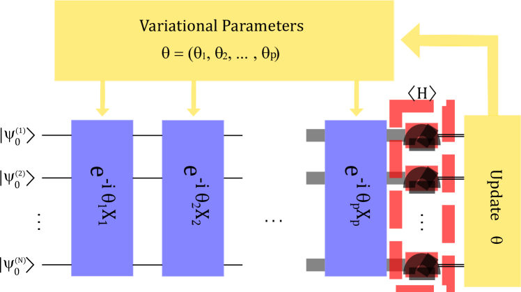
Figure 1: Variationl hybrid quantum-classical optimization. A quantum computer is used to prepare the variational state (2) by sequentially applying some gates that depend on parameters $\theta_{j}$, and then to measure the observable $\hat{H}$ to estimate the cost (1). A classical algorithm iteratively processes these outcomes and updates the parameters $\theta_{j}$ to iteratively minimize the cost (1).

Variational hybrid quantum-classical algorithms, schematically shown in Fig. (1), operate iteratively a quantum device and a classical processor. At the $i$-th iteration, the quantum device generates the variational state $\ket{\psi(\boldsymbol{\theta}^{(i)})}=e^{-i\theta^{(i)}_{P}\hat{X}_{P}}\cdots e^{-i\theta^{(i)}_{1}\hat{X}_{1}}\ket{\psi(\boldsymbol{\theta}^{(i-1)})}$, and estimate the cost (1), and possibly its derivatives $\partial_{\theta_{j}}C$, via quantum measurements Mitarai et al. (2018); Schuld et al. (2019); Harrow and Napp (2019) of the observable $\hat{H}$. This is the computationally hardest part, as it requires the manipulation of states that belong to Hilbert spaces whose dimension exponentially increases with the number of qubits $N$. Afterwards, a classical algorithm processes the estimated values of $C(\boldsymbol{\theta}^{(i)})$, or derivatives $\partial_{\theta_{j}}C$, and proposes new parameters $\boldsymbol{\theta}^{(i+1)}$ that are expected to flow towards the minimum of the cost function. Classical optimization, quantum evolution, and quantum measurements are thus performed iteratively till convergence. The advantage of this hybrid approach is that the quantum computer is always reset after each iteration so that the coherence times required are just those necessary to operate a circuit with depth $\mathcal{O}(P)$ and then perform a measurement.

The main difference with other common variational approaches used in quantum mechanics is that $C(\boldsymbol{\theta})$, or derivatives $\partial_{\theta_{j}}C$, are estimated from measurement outcomes and, as such, are affected by uncertainty due to the probabilistic nature of quantum measurements, even in the noiseless case.

Having access to stochastic values of the cost function dramatically changes the convergence time Bubeck et al. (2015). Algorithms for stochastic optimization are classified as zeroth-order, or derivative-free, when only $C(\boldsymbol{\theta})$ is measured, first-order when it is possible to directly measure the derivatives w.r.t. $\theta_{j}$ of the cost function or, in general, $k$th-order when also $k$th-order derivatives are available. It has been recently shown Harrow and Napp (2019) that first-order methods can lead to substantially faster convergence than zeroth-order methods. On the other hand, the convergence time is not more strictly bounded when using higher-order derivatives, although some advantage may be observed in practical implementations. Motivated by that analysis, here we focus on the convergence of first-order methods using the framework of stochastic optimization.

When dealing with stochastic optimization problems, where only the stochastic outcomes $f(\boldsymbol{\theta},y)$ are directly measurable by sampling different values of $y$ that are distributed according to a distribution $p(y|\boldsymbol{\theta})$, the cost function is usually written Kingma and Ba (2014); Bubeck et al. (2015); Harrow and Napp (2019) as $C(\boldsymbol{\theta})=\mathbb{E}_{y\sim p(y|\boldsymbol{\theta})}[f(\boldsymbol{\theta},y)]$, where $\mathbb{E}_{y\sim p(y|\boldsymbol{\theta})}[f(\boldsymbol{\theta},y)]$ is the expectation value $\sum_{y}p(y|\boldsymbol{\theta})f(\boldsymbol{\theta},y)$. The cost function (1) can be written in the above form by using the (possibly unknown) eigendecomposition of $\hat{H}\equiv\sum_{y}E_{y}\ket{y}\!\bra{y}$: the measurement outcomes $y$ are distributed with probability $p(y|\boldsymbol{\theta})=\bra{y}\hat{\rho}(\boldsymbol{\theta})\ket{y}$, where $\hat{\rho}(\boldsymbol{\theta})=\ket{\psi(\boldsymbol{\theta})}\!\bra{\psi(\boldsymbol{\theta})}$, and $f(\boldsymbol{\theta},y)=E_{y}$ is the associated cost, which is independent of $\boldsymbol{\theta}$.

When the eigendecomposition of $\hat{H}$ is not known, one can still get $C(\boldsymbol{\theta})$ from Pauli measurements, namely by decomposing $\hat{H}$ as $\hat{H}=\sum_{\mu=1}^{L}h_{\mu}\hat{\sigma}_{\mu}$ where each $\hat{\sigma}_{\mu}$ is a tensor product of Pauli matrices and $h_{\mu}$ the corresponding coefficient, and then by independently estimating each $\langle\psi(\boldsymbol{\theta})|\hat{\sigma}_{\mu}|\psi(\boldsymbol{\theta})\rangle$. Note that many $\hat{\sigma}_{\mu}$ typically commute with each other, so the required number of independent measurements can be smaller than $L$.

Suppose now that $\boldsymbol{\nabla}C(\boldsymbol{\theta})=\mathbb{E}_{z\sim q(z|\boldsymbol{\theta})}[\boldsymbol{g}(\boldsymbol{\theta},z)]$, with $\nabla_{j}:=\frac{\partial}{\partial\theta_{j}}$, i.e. that the gradient of $C$ can be written as an expectation of a vector-valued function $\boldsymbol{g}(\boldsymbol{\theta},z)$ over some stochastic outcomes $z$, distributed with a probability distribution $q$, possibly different from $p$. The simplest first-order method for stochastic optimization is stochastic gradient descent (SGD) that, intuitively, acts as a gradient descent algorithm where $\boldsymbol{\nabla}C$ is substituted with an unbiased estimate $\boldsymbol{g}$. If the parameters are updated at each iteration $i$ as $\boldsymbol{\theta}^{(i+1)}=\boldsymbol{\theta}^{(i)}-\alpha_{i}\boldsymbol{g}(\boldsymbol{\theta}^{(i)})$ then, after $I$ iterations, the algorithm converges Bubeck et al. (2015); Harrow and Napp (2019); Ruppert (1988); Polyak and Juditsky (1992) to a local optimum $\boldsymbol{\theta}^{\rm opt}$ with

$$\mathbb{E}[C(\boldsymbol{\theta}^{[1:I]})]-C(\boldsymbol{\theta}^{\rm opt})\leq R\frac{G}{\sqrt{I}}~{}.$$ (3)

The left-hand side of (3), where $\boldsymbol{\theta}^{[1:I]}=\frac{1}{I}\sum_{i=1}^{I}\boldsymbol{\theta}^{(i)}$, formally defines what we call “accuracy” in this work; in the right-hand side of the inequality $R$ is a constant that depends on the function and on the parameter space, while $G$ is an upper bound on the norm of the gradient estimate, $\mathbb{E}[\|\boldsymbol{g}(\boldsymbol{\theta})\|_{2}^{2}]\leq G^{2}$. Such rate is achieved with $\alpha_{i}\equiv\alpha=RI^{-1/2}/G$. The inequality (3) means that a larger gradient variance implies slower convergence. Note that, due to the stochastic nature of $\boldsymbol{g}$, even the parameters $\boldsymbol{\theta}^{(i)}$ are stochastic. On the other hand, Eq. (3) shows that $\boldsymbol{\theta}^{[1:I]}$ is a good estimator of the optimal value $\boldsymbol{\theta}^{\rm opt}$ in the limit of many iterations $I$, and an arbitrarily small error $\epsilon\propto G/\sqrt{I}$ may be achieved. In other algorithms Bubeck et al. (2015); Kingma and Ba (2014); Harrow and Napp (2019), the convergence depends on the bound $\mathbb{E}[\|\boldsymbol{g}(\boldsymbol{\theta})\|_{\infty}^{2}]\leq G_{\infty}^{2}$, obtained with a different norm. Since norm inequalities imply $G\leq\sqrt{P}G_{\infty}$, we can always focus on $G_{\infty}$. Although different algorithms may have different convergence times, for instance with adaptive $\alpha_{i}$ and other definitions of $\boldsymbol{\theta}^{[1:I]}$, most upper bounds have a form similar to (3). Faster convergence, $\epsilon\approx G^{2}/I$, can be obtained when $C(\boldsymbol{\theta})$ satisfies extra properties Bubeck et al. (2015); Harrow and Napp (2019), such as strong convexity, with a slightly different definition of $\boldsymbol{\theta}^{[1:I]}$. The bound (3) assumes that the parameters are updated after each query, namely after a single measurement outcome $\boldsymbol{g}$. An alternative is mini-batch learning Bubeck et al. (2015), where $M>1$ queries are used to better estimate the gradient. Although this yields a less-noisy gradient estimator, which for instance provides better numerical results in training quantum dynamical systems Banchi et al. (2016); Innocenti et al. (2019), the theoretical worst-case convergence rate is similar to (3). Indeed, a bound like (3) can be written with $I=MN_{\rm iter}$, with $N_{\rm iter}$ the number of iterations and $I$ the total number of measurements.

III Hybrid optimization with noisy operations

Due to the unavoidable errors in their operation, NISQ devices cannot exactly prepare the ideal variational state (2), which must hence be substituted with $\hat{\rho}(\boldsymbol{\theta})=\mathcal{E}(\boldsymbol{\theta})[\hat{\rho}_{0}]$, where $\hat{\rho}_{0}$ is the noisy version of $\ket{\psi_{0}}$ and $\mathcal{E}(\boldsymbol{\theta})$ the noisy dynamical map. Although most of our theoretical bounds hold for more complex noise models, for the sake of simplicity in the following we use the decomposition

$$\hat{\rho}(\boldsymbol{\theta})=\mathcal{E}^{\theta_{P}}_{P}\circ\cdots\circ\mathcal{E}^{\theta_{1}}_{1}[\hat{\rho}_{0}]~{},$$ (4)

where $\circ$ indicates composition and $\mathcal{E}_{j}^{\theta_{j}}$ is the noisy version of the ideal parametric unitary channel $\mathcal{U}_{j}^{\theta_{j}}[\hat{\rho}]=e^{-i\theta_{j}\hat{X}_{j}}\hat{\rho}e^{i\theta_{j}\hat{X}_{j}}$ implemented by the $j$-th parametric gate of the NISQ device. In what follows, $C_{\rm min}:=\min_{\psi}\langle\psi|H|\psi\rangle$ is the exact minimum of the cost function. Since $\hat{\rho}(\boldsymbol{\theta})$ is a mixed state, the minimization of the cost function $C_{\rm noisy}(\boldsymbol{\theta}):=\Tr[\hat{\rho}(\boldsymbol{\theta})\hat{H}]$ only provides an approximation to the minimum $C(\boldsymbol{\theta}^{\rm opt})$ that can be obtained in the noiseless case. Although not explicitly considered in this paper, our analysis may be straightforwardly extended to some cases where even the ideal target is a mixed state, e.g. the non-equilibrium steady state of a noisy evolution Yoshioka et al. (2019); Carollo et al. (2019); Banchi et al. (2014).

The convergence rate of stochastic optimization towards the noisy minimum $C_{\rm noisy}(\boldsymbol{\vartheta}^{\rm opt.})$, with optimal parameters $\boldsymbol{\vartheta}^{\rm opt}$, can be bounded as in Eq. (3). Considering both the error due to the finite number of iterations and the error due to the difference between $C(\boldsymbol{\theta}^{\rm opt})$ and $C_{\rm noisy}(\boldsymbol{\vartheta}^{\rm opt})$ we may write

$$C_{\rm noisy}(\boldsymbol{\theta}^{[1:I]})-C(\boldsymbol{\theta}^{\rm opt})\leq{\rm Err}(\boldsymbol{\theta}^{\rm opt},\boldsymbol{\vartheta}^{\rm opt})+R\frac{G^{\rm noisy}}{\sqrt{I}}~{},$$ (5)

where we define ${\rm Err}(\boldsymbol{\theta},\boldsymbol{\vartheta})$ as the difference between the noisy and noiseless costs, namely

$${\rm Err}(\boldsymbol{\theta},\boldsymbol{\vartheta}):=C_{\rm noisy}(\boldsymbol{\vartheta})-C(\boldsymbol{\theta})~{}.$$ (6)

For some noise models, it can be shown that $\boldsymbol{\vartheta}^{\rm opt}=\boldsymbol{\theta}^{\rm opt}$, namely that the optimal parameters in the noiseless and noisy case are the same Sharma et al. (2019). The inequality (5) shows a simple and yet important aspect: after a fixed number of iterations $I$, our best approximation to the noiseless variational minimum has an error that is given by two different terms. The first one follows from the difference between the noiseless and noisy case, while the second one depends on the gradient estimator and always decreases for increasing $I$. To simplify our discussion and provide a worst-case scenario, we assume that we know how to choose an ideal variational ansatz (2) that provides $C_{\rm min}=C(\boldsymbol{\theta}^{\rm opt})$, and consequently ensures ${\rm Err}(\boldsymbol{\vartheta}^{\rm opt},\boldsymbol{\theta}^{\rm opt})\geq 0$. This is typically not the case, as variational ansatze are normally chosen as simple circuits that are easy to implement on a NISQ device, for which one might get a negative ${\rm Err}(\boldsymbol{\vartheta}^{\rm opt},\boldsymbol{\theta}^{\rm opt})$. The worst-case error coming from the first term in the r.h.s. of (5) can be bounded by adapting the “peeling” technique from Pirandola et al. (2017, 2018). Indeed, we show in the Appendix A that ${\rm Err}(\boldsymbol{\theta},\boldsymbol{\vartheta})\leq P\|\hat{H}\|_{\infty}\max_{k}\|\mathcal{E}_{k}^{\vartheta_{k}}-\mathcal{U}_{k}^{\theta_{k}}\|_{\diamond}$ so the error increases at most linearly with the depth $P$ and depends on the maximum distance, as measured by the diamond norm Kitaev (1997); Watrous (2018), between the ideal gates and their noisy implementations – see also Eq. (15). An alternative inequality ${\rm Err}(\boldsymbol{\theta},\boldsymbol{\vartheta})\leq 2\|\hat{H}\|_{\infty}\;\sqrt{1-\bra{\psi(\boldsymbol{\theta})}\hat{\rho}(\boldsymbol{\vartheta})\ket{\psi(\boldsymbol{\theta})}}$ shows that the first error term is bounded by the fidelity between the optimal pure state and its noisy version.

We now focus on $G^{\rm noisy}$ in (5), which depends on the procedure used to estimate the gradient from quantum measurements. The measurement of an observable with associated operator $\hat{g}_{j}$ provides an unbiased estimator of the gradient if $\nabla_{j}C=\Tr[\hat{\rho}\hat{g}_{j}]$ for each $j$. In this sense, we refer to the observables $\hat{g}_{j}$ as estimators of the gradient. In the noiseless case different estimators have been proposed McClean et al. (2018); Mitarai et al. (2018); Schuld et al. (2019); Harrow and Napp (2019), based on either the Hadamard test or the so-called parameter-shift rule. However, those estimators may result biased if only noisy gates are available: therefore, a rigorous generalization to the noisy regime is still lacking. The convergence of SGD with biased gradient estimators is not much understood, aside from specific algorithms such as simultaneous perturbation stochastic approximation (SPSA) Spall et al. (1992), where the bias can be controlled. In order to define an unbiased estimator in the general case we use the geometry of quantum states, from which we know that any derivative can be written as Paris (2009); Bengtsson and Życzkowski (2017)

$$\nabla_{j}\hat{\rho}=\frac{\hat{L}_{j}\hat{\rho}+\hat{\rho}\hat{L}_{j}}{2}~{},$$ (7)

where the operator $\hat{L}_{j}$ is called the symmetric logarithmic derivative (SLD). The gradient of the cost $C(\boldsymbol{\theta})=\Tr[\hat{\rho}(\boldsymbol{\theta})\hat{H}]$ can hence be obtained by measuring observables with associated operators

$$\hat{g}_{j}(\boldsymbol{\theta})=\frac{\hat{L}_{j}(\boldsymbol{\theta})\hat{H}+\hat{H}\hat{L}_{j}(\boldsymbol{\theta})}{2}+\lambda_{j}\hat{L}_{j}(\boldsymbol{\theta})~{},$$ (8)

for any $\lambda_{j}$. The freedom in choosing $\lambda_{j}$ follows from Eq. (7), as $\Tr[\hat{L}_{j}\hat{\rho}]=\Tr[\nabla_{j}\hat{\rho}]=\nabla_{j}\Tr[\hat{\rho}]=0$ implies that the expectation value $\nabla_{j}C=\Tr[\hat{g}_{j}\hat{\rho}]$ is independent of $\lambda_{j}$. Therefore, the free parameters $\lambda_{j}$ are analogous to the so-called baselines, commonly employed in reinforcement learning for variance reduction Deisenroth et al. (2013). The optimal $\lambda_{j}$s are discussed in Appendix B. The measurement of the gradient operators provides stochastic outcomes $g^{\rm SLD}_{j}(\boldsymbol{\theta},\gamma)$ with probabilities $\langle{g_{\gamma,j}}|\hat{\rho}|{g_{\gamma,j}}\rangle$, where we used the eigendecomposition $\hat{g}_{j}{=}\sum_{\gamma}g^{\rm SLD}_{j}(\boldsymbol{\theta},\gamma)|{g_{\gamma,j}}\rangle\!\langle{g_{\gamma,j}}|$. For pure states, the SLD operator has a simple form $\hat{L}_{j}=\ket{\psi(\boldsymbol{\theta})}\langle{\nabla_{j}\psi(\boldsymbol{\theta})}|$ and the above estimation strategy becomes equivalent to others, proposed in the literature McClean et al. (2018); Mitarai et al. (2018); Schuld et al. (2019); Harrow and Napp (2019), which can be explicitly measured using a generalization of the Hadamard test Harrow and Napp (2019).

An alternative estimator can be obtained using the log-derivative (LD) trick Glynn (1990), also called “reinforce” in the machine learning literature Williams (1992), which consists in writing the gradient of the cost function $\nabla_{j}C=\sum_{y}E_{y}\nabla_{j}p(y|\boldsymbol{\theta})$ as en expectation value of $g^{\rm LD}_{j}(\boldsymbol{\theta},y)=E_{y}\nabla_{j}\log p(y|\boldsymbol{\theta})$ over the original distribution $p(y|\boldsymbol{\theta})=\bra{y}\hat{\rho}(\boldsymbol{\theta})\ket{y}$ where $\hat{H}=\sum_{y}E_{y}\ket{y}\!\bra{y}$.

In Appendix C, we show that all different estimators for the gradient satisfy the upper bound

$$G^{\rm noisy}\leq\sqrt{P}G^{\rm noisy}_{\infty}\leq\sqrt{P}\|\hat{H}\|_{\infty}\max_{j,\boldsymbol{\theta}}\sqrt{{\rm QFI}_{j}(\boldsymbol{\theta})}~{},$$ (9)

where QFI is the Quantum Fisher Information

$${\rm QFI}_{j}(\boldsymbol{\theta})=\Tr[\hat{\rho}(\boldsymbol{\theta})\hat{L}_{j}(\boldsymbol{\theta})^{2}]~{},$$ (10)

a central quantity in quantum metrology Paris (2009) that is also relevant for studying quantum phase transitions Zanardi et al. (2007); Venuti and Zanardi (2007); Banchi et al. (2014).

Before proceeding further, let us briefly comment upon the emergence of the QFI in this context. There are two slightly different way of understanding the QFI. First, there is the QFI of a state $\hat{\rho}$ with respect to a certain observable $\hat{X}$: this is $F_{Q}[\hat{\rho},\hat{X}]:=2\sum_{mn}\frac{(\rho_{m}-\rho_{n})^{2}}{(\rho_{m}+\rho_{n})}|\bra{m}\hat{X}\ket{n}|^{2}$, where $\hat{\rho}=\sum_{n}\rho_{n}\ket{n}\!\bra{n}$ is the eigendecomposition of $\hat{\rho}$. When $\hat{\rho}$ is a pure state, the QFI is nothing but twice the expectation value of $\hat{X}$ on such state. On the other hand, if it exist a reference state $\hat{\rho}_{0}$ and a real parameter $\theta$ (that we here take as one-dimensional for the sake of clarity) such that $\hat{\rho}=e^{-i\theta\hat{X}}\hat{\rho}_{0}e^{i\theta\hat{X}}\>=\hat{\rho}(\theta)$, then it is $F_{Q}[\hat{\rho},\hat{X}]=F_{Q}[\hat{\rho}(\theta)]={\rm Tr}[\hat{\rho}(\theta)\hat{L}^{2}]$, where $\hat{L}$ is the LSD we have encounterd above, whose relation with the observable $\hat{X}$ is via $i[\hat{\rho},\hat{X}]=\frac{1}{2}(\hat{L}\hat{\rho}+\hat{\rho}\hat{L})$. The expression $F_{Q}[\hat{\rho}(\theta)]$ is common in quantum metrology, where it quantifies the sensitivity of the parametric state $\hat{\rho}(\theta)$ to the variations of $\theta$ itself. To this respect notice that if $\theta$ represents the classical quantity to be measured via a quantum-metrology protocol, a higher QFI guarantees a more precise result. The above comments are easily generalized to the case of a multidimensional parameter $\boldsymbol{\theta}$ as the one used elsewhere in this work.

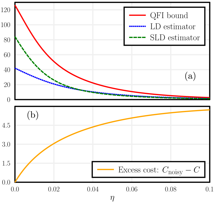
Figure 2: Opposite behaviour of the two sources of error. (a) the square root of second statistical moment of the gradient estimator $\max_{\boldsymbol{\theta}}\sqrt{\mathbb{E}[\|\boldsymbol{g}(\boldsymbol{\theta})\|_{2}^{2}]}\leq G_{\rm noisy}$ and (b) the excess cost ${\rm Err}(\boldsymbol{\theta}^{\rm opt},\boldsymbol{\vartheta}^{\rm opt})$, as a function of the depolarising noise strength $\eta$ (see Sec. IV for the definition of $\eta$). The variational circuit corresponds to a QAOA for a ring of $N=6$ qubits with $20$ variational parameters. Different gradient estimators are considered: the one based on the log-derivative trick (LD) and the one based on the symmetric logarithmic derivative (SLD). Those are plotted against the upper bound (9) based on the Quantum Fisher Information (QFI).

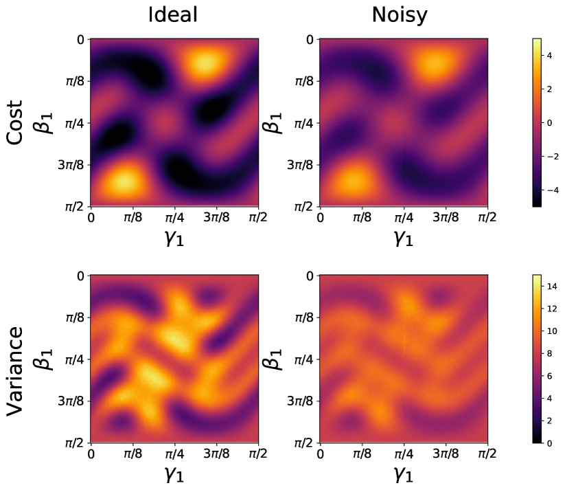
Figure 3: Typical form of the cost-function landscape in the noiseless (left) to the noisy (right) regimes as a function of two parameters, $\gamma_{1}$ and $\beta_{1}$ – see Sec. IV for the model description. Costs $\langle\hat{H}\rangle$ and variances $\langle\hat{H}^{2}\rangle-\langle\hat{H}\rangle^{2}$ are respectively shown in the top and bottom panels.

Let us now get back to the bound (9) to underline a very important aspect: while the first term in the r.h.s. of (5) increases as a function of the noise strength, the second one can decrease. Indeed, it is known that noise is normally detrimental for metrology, as it can reduce the QFI from $\mathcal{O}(N^{2})$ (Heisenberg limit) to $\mathcal{O}(N)$ (standard quantum limit) Escher et al. (2011); Giovannetti et al. (2011). Our analysis thus shows that the convergence accuracy, as defined by the l.h.s. of (5), is bounded by the sum of two terms that typically display opposite behaviours as a function of the noise strength, with the first one increasing and the second one decreasing, as shown in Fig. 2 for the specific example that will be described in the following section. From the physical point of view, this is due to how the cost-function landscape is affected by noise. As shown in Fig. 3 for strong noise the landscape is “flattened”, and hence the minimum cost is higher, but so does the variance, and hence the maximum variance is lower. Therefore, in the noisy regime the number of operations needed in order to correctly find the minimum may be reduced. Our analysis of Eq. (5) quantifies this intuition: when the number of iterations $I$ is small, we may observe that noise is actually beneficial. However, due to measurement uncertainty, the number of iterations required for convergence is typically large and $I\gg\sqrt{P}R^{2}{\rm QFI}$. In this regime noise is always detrimental, as observed in some numerical experiments Xue et al. (2019); Alam et al. (2019).

The bound (5), together with the above analysis, shows that the convergence speed is mostly unaffected by noise, while the quality of the solution typically deteriorates due to the error ${\rm Err}(\boldsymbol{\theta},\boldsymbol{\vartheta})$, which still increases at most linearly with the depth $P$ of the circuit. Therefore, we may expect that hybrid variational optimization is robust against noise. In the next section we numerically study such robustness for a relevant optimization problem.

IV Numerical examples

QAOA Farhi et al. (2014) is a specific ansatz for variational hybrid optimization which consists in the repetition of two types of parametric quantum evolutions generated by two different non-commuting Hamiltonians, typically called $\hat{H}_{\gamma}$ and $\hat{H}_{\beta}$. Here $\hat{H}_{\gamma}\equiv\hat{H}$ is equal to the cost operator appearing in Eq. (1) and is a function of the Pauli $\hat{\sigma}^{z}_{l}$ operators only, where the indices $l=1,\dots,N$ refer to the different qubits. In the computational basis defined by the eigenstates $\{\ket{0},\ket{1}\}$ of $\hat{\sigma}_{l}^{z}$, $H$ is diagonal. The other Hamiltonian is fixed as $\hat{H}_{\beta}=-\sum_{l}\hat{\sigma}^{x}_{l}$, where $\hat{\sigma}_{l}^{x}$ are other Pauli operators, which are not diagonal in the computational basis. The QAOA evolution can be written as in Eq. (2) with sequential applications of $\hat{H}_{\gamma}$ and $\hat{H}_{\beta}$

$$\ket{\psi(\boldsymbol{\gamma},\boldsymbol{\beta})}=e^{-i\beta_{\cal P}\hat{H}_{\beta}}e^{-i\gamma_{\cal P}\hat{H}_{\gamma}}\cdots e^{-i\beta_{1}\hat{H}_{\beta}}e^{-i\gamma_{1}\hat{H}_{\gamma}}\ket{+}^{\otimes N}~{}.$$ (11)

The parameters are then split as $\boldsymbol{\theta}=(\boldsymbol{\gamma},\boldsymbol{\beta})$ and the total depth of the circuit is $P=2{\cal P}$. The initial state $\ket{\psi_{0}}=\ket{+}^{\otimes N}$, where $\ket{+}=(\ket{0}+\ket{1})/\sqrt{2}$, is the ground state of $\hat{H}_{\beta}$. QAOA is a universal model for quantum computation Lloyd (2018); Morales et al. (2019), meaning that, with specific choices of $\hat{H}_{\gamma}$, any state can be arbitrarily well approximated by $\ket{\psi(\boldsymbol{\gamma},\boldsymbol{\beta})}$ with suitable parameters $\gamma_{j}$, $\beta_{j}$ and ${\cal P}\to\infty$. For the specific choice $\gamma_{j}\propto j/{\cal P}$ and $\beta_{j}\propto(1-j/{\cal P})$, Eq. (11) can be interpreted as a discretization of an adiabatic evolution Barends et al. (2016); Farhi et al. (2014) and QAOA is guaranteed to perform well for large enough ${\cal P}$. The QFI can be large when the adiabatic evolution crosses a dynamical phase transition Zanardi et al. (2007); Venuti and Zanardi (2007); Banchi et al. (2014) and the error from $G_{\rm noisy}$ in (5) can be significant when the Hamiltonian $\beta\hat{H}_{\beta}+\gamma\hat{H}_{\gamma}$ displays a quantum phase transition for some choices of $(\beta,\gamma)$. One such example is the Ising ring Lieb et al. (1961) studied below, where $\hat{H}_{\beta}$ models the global transverse field. In such model, the QFI scales as $\mathcal{O}(N^{2})$ in the translational invariant case, while for steady states of more complex noisy evolution it can be as large as $\mathcal{O}(N^{6})$ Banchi et al. (2014).

Here we study QAOA applied to a translational invariant antiferromagnetic ring with $\hat{H}_{\gamma}=\sum_{l=1}^{N}\hat{\sigma}_{l}^{z}\hat{\sigma}_{l+1}^{z}$ and periodic boundary conditions $\hat{\sigma}^{z}_{N+1}\equiv\hat{\sigma}^{z}_{1}$. QAOA with this model has been studied in Wang et al. (2018); Mbeng et al. (2019), using the exact mapping to a free-fermion model. In particular, it has been proven Wang et al. (2018) that the ground state can be exactly expressed with the QAOA ansatz (11) as long as ${\cal P}\geq N/2$. The effect of noise in an overparameterized QAOA is shown in Fig. 2, where we consider the effect of a local depolarising error, as in (4) with $\mathcal{E}_{j}^{\theta_{j}}[\hat{\rho}]=\mathcal{D}[e^{-i\theta_{j}\hat{X}_{j}}\hat{\rho}e^{i\theta_{j}\hat{X}_{j}}]$, $\mathcal{D}=\bigotimes_{l=1}^{N}\mathcal{D}_{l}$ and $\mathcal{D}_{l}(\rho)=(1-\eta)\hat{\rho}+\eta\hat{\sigma}_{l}^{z}\hat{\rho}\hat{\sigma}_{l}^{z}$. All bounds are computed by numerically finding the operators $\hat{L}_{j}$ from Eq. (7). In Fig. 2 we see that our theory predicts a decreasing $G_{\rm noisy}$ in (5) as a function of $\eta$. In Appendix D we also study a different noise model, where the NISQ computer implements noisy yet unitary gates $e^{-i(\theta_{j}+\eta\epsilon_{j})X_{j}}$ where $\epsilon_{j}\sim\mathcal{N}(0,1)$ is a Gaussian random variable. We found that also with this noise, the error terms display the same behaviour shown in Fig. 2.

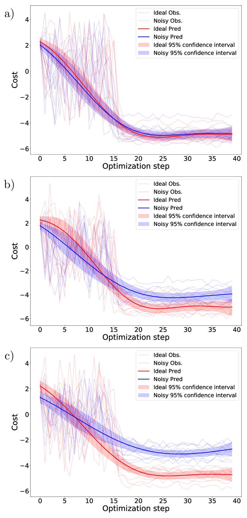
Figure 4: Numerical results on the convergence of QAOA. We use $N=8$ and ${\cal P}=3$ in all panels a), b) and c). Red and blue curves, respectively, represent noiseless and noisy evolution. The noise parameters are taken from typical values of IBM quantum processors (see Appendix E), yet increased by a factor 2 (panel a), a factor 4 (panel b) and a factor 10 (panel c). The convergence of the cost function (1) is shown during the optimization procedure; faded thin lines are ten trials of the same realization of QAOA,while solid lines show the empirical average evolution from the ten trials. For more information, see the main text.

We test our theoretical predictions using the Qiskit framework Abraham et al. (2019) to simulate QAOA on a physical hardware by numerical experiments. In these simulations, the error model consists of single- and two-qubit gate errors, i.e. depolarizing error followed by a thermal relaxation error, as discussed in Appendix E. In Fig. 4 we show the optimization of the cost function (1) using a simple gradient descend update, where each gradient value is estimated by using a quantum circuit followed by local measurements (see Appendix F for details); these operations are repeated 200 times to estimate a single value. Due to the stochastic measurement outcomes, each optimization takes a different stochastic route. Fig. 4 is divided into three panels, a), b) and c), differing from each other only for noise strength. In fact, in order to study the performance of QAOA in different noisy regimes, we progressively increase noise strength in our simulations: in the results reported in Fig. 4 noise strength has been progressively increased by factor $f=2$ (panel a), a factor $f=4$ (panel b), and a factor $f=10$ (panel c), namely gate errors, relaxation and decoherence rates are all increased by the factor $f$ compared to the typical values of noise parameters obtained from IBM quantum processors (see Appendix E). Results obtained without increase, namely with $f=1$, are not reported, since they are basically indistinguishable from those obtained in the noiseless case. We expect that noise effects can become visible even with $f=1$ when the number of qubits $N$ and/or circuit depth $P$ are sensibly larger than those employed in our simulations.

The following description holds for all three individual panels regardless of the increase factor $f$ of noise strength: the fade thin lines correspond to ten different trials of optimization of the cost function in both noisy (blue) and noiseless (red) cases with the same initial conditions. We observe that the cost, estimated alike the gradient repeating 200 times the quantum circuit and measurements, initially highly fluctuates between different runs, but then all runs converge towards the local minimum (since ${\cal P}<N/2$ the global minimum cannot be achieved). Higher accuracy in the convergence may be obtained using more sophisticated first order methods Kingma and Ba (2014). Optimizations starting from different initial parameters display a similar behaviour (not shown). Using Gaussian process regression we have also computed average “path-integral-like” optimization curves, which are shown in the same graph in Fig. 4 with solid lines for both the noiseless and noisy cases. These lines show the empirical average evolution from the ten trials, and colored zones represent 95% confidence intervals associated with such average.

We observe that for small noise strength, e.g. panel a) in Fig. 4, the average optimization curves are basically indistinguishable from the noisy ones, aside from finite-size effects due to the finite number of measurements. For moderate noise values, panel b) in Fig. 4, as predicted by our theory, the final point in the optimization is slightly higher in the noisy regime, but the convergence speed is comparable. Moreover, at the initial points, the average cost is smaller in the noisy case. Although this prediction may be due to the finite number of curves, it is consistent with our analysis from (5). For large noise strengths, panel c) in Fig. 4, we observe that the final cost significantly deviates from the noiseless case, but the convergence speed is again comparable.

Overall our analysis shows that the convergence speed of hybrid variational optimization is not significantly affected by noise, while the quality of the final solution is.

V Discussion

We have studied the convergence speed of variational hybrid quantum-classical optimization algorithms, showing that the error after a finite number of steps can be upper-bounded by the sum of two terms: the first one is the difference between the noisy and the noiseless result, and typically increases for stronger noise; the second term, though, is proportional to the square root of the quantum Fisher information, that usually decreases with noise. Due to the competition between these two terms, depending on the noise strength, different results can be observed. For small to intermediate noise we find that the convergence time is mostly unaffected by the presence of noise; This said, for a number of iterations such that the convergence time has not passed yet, the accuracy may actually be higher in some noisy regimes. On the other hand, if the convergence time is reached, the error term typically dominates, showing the foreseeable negative role of noise.

Let us also comment upon the way QFI enters our results. From the formal viewpoint, we understand its occurrence as due to the use of stochastic optimization methods, which involve the gradient of the cost function with respect to the variational parameters, and hence the operators $\hat{L}_{j}$ in (7), and QFI via its definition (10). However, the substantial reason for the QFI to appear in (9) in a somehow counterintuitive way (the lower the better) can be explained as follows. In estimation theory a larger FI guarantees a better determination of the wanted parameter via the sampling of a function that depends on it; this is because a larger FI follows from larger local values of the derivatives, and hence a higher sensitivity of the overall estimation procedure. On the other hand, in the scheme to which we are referring the role played by the parameter and the sampled function is reversed: we input different values of $\boldsymbol{\theta}$ aiming at exploring the $C(\boldsymbol{\theta})$-landscape, possibly locating its minimum; this exploration is more agile if the above landscape is more level, which corresponds to a lower FI. This general argument holds both in a classical and in a quantum setting, and we think it lies underneath the result Eq. (9) in the following sense: noise can help an algorithmic procedure to more easily explore the landscape of the cost function one wants to minimize, thus increasing, at least as far as its detrimental effect on the cost-function evaluation is not too strong, the overall efficiency of the optimization scheme.

We finally underline that QFI enters our analysis by only providing a theoretical upper bound that never needs being evaluated. In fact, should the QFI be efficiently measurable, one could use more sophisticated stochastic algorithms, such as Amari’s natural gradient Amari (1998); this has been recently applied to noiseless parametric quantum circuits Stokes et al. (2019) based on the fact that, when $C=-\log p(x,\boldsymbol{\theta})$, the natural gradient is Fisher efficient, i.e. such that the variance of the estimator $\boldsymbol{\theta}^{[1:I]}$ asimptotically meets the Cramér-Rao lower bound. However, such a result does not hold for more general cost functions like (1). Furthermore, no efficient method (e.g. poly$(N)$) for estimating the QFI from measurements is currently available in the noisy regime and, even if it existed, estimating the QFI at each step would require further quantum measurements that would increase the query complexity. In fact, understanding whether one can obtain Fisher efficient estimators of the optimal parameters is currently an open question.

Appendix A Bound on ${\rm Err}(\boldsymbol{\theta},\boldsymbol{\vartheta})$

Many of our results hold irrespective of assumption (4), and are valid for any error model

$$\hat{\rho}(\boldsymbol{\theta})=\mathcal{E}(\theta_{1},\dots,\theta_{P})[\hat{\rho}_{0}]~{}.$$ (12)

Indeed, all results that we derive in appendices B, C do not depend on the assumption (4) and are valid for any noise model as in (12). Here we show on the other hand that when the local error model (4) is assumed, then the error ${\rm Err}(\boldsymbol{\theta},\boldsymbol{\vartheta})$ grows at most linearly with the number of parameters. We study an upper bound to the first error in (5), which is clearly valid irrespective of the sign of ${\rm Err}(\boldsymbol{\theta},\boldsymbol{\vartheta})$

$${\rm Err}(\boldsymbol{\theta},\boldsymbol{\vartheta}) :=\Tr[\hat{H}(\hat{\rho}(\boldsymbol{\vartheta})-\ket{\psi(\boldsymbol{\theta})}\!\bra{\psi(\boldsymbol{\theta})})]$$

$$\stackrel{{\scriptstyle(a)}}{{\leq}}\|\hat{H}\|_{\infty}\;\|\hat{\rho}(\boldsymbol{\vartheta})-\ket{\psi(\boldsymbol{\theta})}\!\bra{\psi(\boldsymbol{\theta})}\|_{1}$$

$$\stackrel{{\scriptstyle(b)}}{{\leq}}\|\hat{H}\|_{\infty}\;\|\mathcal{E}(\boldsymbol{\vartheta})-\mathcal{U}(\boldsymbol{\theta})\|_{\diamond}~{},$$ (13)

where $\|\hat{X}\|_{\infty}$ is the maximum singular value of $\hat{X}$, namely the maximum absolute value $|x_{j}|$ where $x_{j}$ are the eigenvalues of $\hat{X}$, $\|\hat{X}\|_{1}=\Tr[\sqrt{\hat{X}\hat{X}^{\dagger}}]$ is the trace norm, and $\|\mathcal{X}\|_{\diamond}$ is the diamond norm for quantum channels Kitaev (1997); Watrous (2018). In the last line it is

$$\mathcal{U}(\boldsymbol{\theta}) :=\mathcal{U}_{P}^{\theta_{P}}\circ\cdots\circ\mathcal{U}_{1}^{\theta_{1}}~{},$$ (14)

and

$$\hat{\rho}(\boldsymbol{\vartheta}) =\mathcal{E}(\boldsymbol{\vartheta})[\ket{\psi_{0}}\!\bra{\psi_{0}}]~{}, \ket{\psi(\boldsymbol{\theta})}\!\bra{\psi(\boldsymbol{\theta})} =\mathcal{U}(\boldsymbol{\theta})[\ket{\psi_{0}}\!\bra{\psi_{0}}]~{},$$

where for simplicity we have absorbed the noisy preparation of $\ket{\psi_{0}}$ into $\mathcal{E}_{1}$. To derive (13), in (a) we used the Hölder inequality and in (b) we used the distance induced by the diamond norm

$$\|\mathcal{E}-\mathcal{U}\|_{\diamond}=\max_{\rho}\|\mathcal{I}\otimes\mathcal{E}(\rho)-\mathcal{I}\otimes\mathcal{U}(\rho)\|_{1}~{},$$ (15)

where $\mathcal{I}$ is the identity channel. We can now apply the “peeling” technique from Pirandola et al. (2017, 2018) to bound the error in the diamond distance. To this aim, we now use the decomposition from Eq. (4) from the main text, and let $\delta_{P}=\|\mathcal{E}_{1:P}-\mathcal{U}_{1:P}\|_{\diamond}$, where the $1{:}k$ refers to the composition of the first $k$ channels. Then, using the monotonicity of the diamond norm over CPTP maps and the triangle inequality, we may write

$$\delta_{P}=$$

$$\|\mathcal{E}_{P}\circ\mathcal{E}_{1:P-1}-\mathcal{E}_{P}\circ\mathcal{U}_{1:P-1}+\mathcal{E}_{P}\circ\mathcal{U}_{1:P-1}-\mathcal{U}_{P}\circ\mathcal{U}_{1:P-1}\|_{\diamond}$$

$$\leq\|\mathcal{E}_{P}\circ\mathcal{E}_{1:P-1}-\mathcal{E}_{P}\circ\mathcal{U}_{1:P-1}\|_{\diamond}+$$

$$\quad+\|\mathcal{E}_{P}\circ\mathcal{U}_{1:P-1}-\mathcal{U}_{P}\circ\mathcal{U}_{1:P-1}\|_{\diamond}$$

$$\leq\delta_{P-1}+\|\mathcal{E}_{P}-\mathcal{U}_{P}\|_{\diamond}~{}.$$

Iteratively applying the above inequality one gets

$$\delta_{P}\leq\sum_{k=1}^{P}\|\mathcal{E}_{k}-\mathcal{U}_{k}\|_{\diamond}\leq P\max_{k}\|\mathcal{E}_{k}-\mathcal{U}_{k}\|_{\diamond}~{}.$$ (16)

Combining (16) and (13) we find that the error increases at most linearly with $P$, according to

$${\rm Err}(\boldsymbol{\theta},\boldsymbol{\vartheta}) \leq P\|\hat{H}\|_{\infty}\max_{k}\|\mathcal{E}_{k}-\mathcal{U}_{k}\|_{\diamond}~{}.$$ (17)

An alternative bound can be obtained from (13) via the Fuchs-van de Graaf inequality Fuchs and Van De Graaf (1999)

$${\rm Err}(\boldsymbol{\theta},\boldsymbol{\vartheta})\leq 2\|\hat{H}\|_{\infty}\;\sqrt{1-\bra{\psi(\boldsymbol{\theta})}\hat{\rho}(\boldsymbol{\vartheta})\ket{\psi(\boldsymbol{\theta})}}~{}.$$ (18)

Appendix B Optimal baselines

We discuss the role of the free parameters $\lambda_{j}$, dubbed “baselines”, in the optimization. In principle, such parameters should be chosen to minimize $\mathbb{E}[g_{j}^{2}]$. We may write

$$\mathbb{E}[g_{j}^{2}] \equiv\left\langle\left(\frac{\{\hat{H},\hat{L}_{j}\}}{2}+\lambda_{j}\hat{L}_{j}\right)^{2}\right\rangle_{\hat{\rho}(\boldsymbol{\theta})}$$ (19)

$$=\left\langle\left(\frac{\{\hat{H},\hat{L}_{j}\}}{2}\right)^{2}+\lambda_{j}\frac{\{\hat{L}_{j},\{\hat{H},\hat{L}_{j}\}\}}{2}+\lambda_{j}^{2}\hat{L}_{j}^{2}\right\rangle_{\hat{\rho}(\boldsymbol{\theta})}$$

$$=\left\langle\left(\frac{\{\hat{H},\hat{L}_{j}\}}{2}\right)^{2}+\lambda_{j}\frac{\{\hat{L}_{j},\{\hat{H},\hat{L}_{j}\}\}}{2}\right\rangle_{\hat{\rho}(\boldsymbol{\theta})}+\lambda_{j}^{2}{\rm QFI}_{j}~{},$$

where $\{\hat{A},\hat{B}\}=\hat{A}\hat{B}+\hat{B}\hat{A}$. Since QFI is always positive, the optimal value of the “baseline” $\lambda_{j}$ is the vertex of the above parabola, namely

$$\lambda^{\rm opt}_{j}=-\frac{\left\langle\{\hat{L}_{j},\{\hat{H},\hat{L}_{j}\}\}\right\rangle_{\hat{\rho}(\boldsymbol{\theta})}}{4{\rm QFI}_{j}}~{}.$$ (20)

We note that the bound (31) continues to hold even when the optimal baseline is used, as by definition $\mathbb{E}[g_{j}^{2}]$ with the optimal baseline is smaller than $\mathbb{E}[g_{j}^{2}]$ for the non-optimal $\lambda_{j}=0$.

Appendix C Bound on $G_{\rm noisy}$

We first focus on the estimator based on the log-derivative trick. We write the cost function as $C=\sum_{y}E_{y}p(y|\boldsymbol{\theta})$, where $p(y|\boldsymbol{\theta})=\bra{y}\hat{\rho}(\boldsymbol{\theta})\ket{y}$, $\hat{H}=\sum_{y}E_{y}\hat{\Pi}_{y}$ is the possibly unknown eigendecomposition of $H$ and $\hat{\Pi}_{y}=\ket{y}\!\bra{y}$. Then

$$\nabla_{j}C=\mathbb{E}_{y\sim p(y|\boldsymbol{\theta})}[E_{y}\nabla_{j}\log p(y|\boldsymbol{\theta})]~{}.$$ (21)

From the above, we find that $g_{j}=E_{y}\nabla_{j}\log p(y|\boldsymbol{\theta})$ is an unbiased estimator of $\nabla_{j}C$. We recall the definition of the constants $G_{\rm noisy}$ and $G_{\infty}$ such that

$$\mathbb{E}\left[\sum_{j}g_{j}^{2}\right] \leq G_{\rm noisy}^{2}~{}, \max_{j}\mathbb{E}\left[g_{j}^{2}\right] \leq G_{\infty}^{2}~{}.$$ (22)

To get those constants we need to find upper bounds for $\mathbb{E}\left[g_{j}^{2}\right]$. By explicit calculation, following a similar derivation of Ref. Paris (2009) we find

$$\mathbb{E}[g_{j}^{2}] =\sum_{y}E_{y}^{2}p(y|\boldsymbol{\theta})[\nabla_{j}\log p(y|\boldsymbol{\theta})]^{2}$$ (23)

$$=\sum_{y}E_{y}^{2}\frac{[\nabla_{j}p(y|\boldsymbol{\theta})]^{2}}{p(y|\boldsymbol{\theta})}$$ (24)

$$\stackrel{{\scriptstyle(a)}}{{=}}\sum_{y}E_{y}^{2}\frac{[\Tr\hat{\Pi}_{y}(\hat{\rho}\hat{L}_{j}+\hat{L}_{j}\hat{\rho})/2]^{2}}{\Tr[\hat{\Pi}_{y}\hat{\rho}]}$$ (25)

$$=\sum_{y}E_{y}^{2}\frac{[\real\Tr(\hat{\Pi}_{y}\hat{\rho}\hat{L}_{j})]^{2}}{\Tr[\hat{\Pi}_{y}\hat{\rho}]}$$ (26)

$$\leq\sum_{y}E_{y}^{2}\frac{\left|\Tr(\hat{\Pi}_{y}\hat{\rho}\hat{L}_{j})\right|^{2}}{\Tr[\hat{\Pi}_{y}\hat{\rho}]}$$ (27)

$$=\sum_{y}E_{y}^{2}\left|\Tr\left(\frac{\sqrt{\hat{\Pi}_{y}}\sqrt{\hat{\rho}}}{\sqrt{\Tr[\hat{\Pi}_{y}\hat{\rho}]}}\sqrt{\hat{\rho}}\hat{L}_{j}\sqrt{\hat{\Pi}_{y}}\right)\right|^{2}$$ (28)

$$\stackrel{{\scriptstyle(b)}}{{\leq}}\sum_{y}E_{y}^{2}\Tr\left(\hat{\Pi}_{y}\hat{L}_{j}\hat{\rho}\hat{L}_{j}\right)$$ (29)

$$=\Tr\left(\hat{H}^{2}\hat{L}_{j}\hat{\rho}\hat{L}_{j}\right)~{},$$ (30)

where in (a) we used the definition of the SLD (7), and in (b) the Cauchy-Schwartz inequality. Using then the Hölder inequality and the fact that $\hat{L}_{j}\hat{\rho}\hat{L}_{j}$ is a positive operator we find then

$$\mathbb{E}[g_{j}^{2}]\leq\|\hat{H}\|_{\infty}^{2}\|\hat{L}_{j}\hat{\rho}\hat{L}_{j}\|_{1}\leq\|\hat{H}\|_{\infty}^{2}{\rm QFI}_{j}~{},$$ (31)

where QFI_j is the Quantum Fisher Information (10). The upper bounds (22) then follows with

$$G =\|\hat{H}\|_{\infty}\sqrt{P\left(\max_{j}{\rm QFI}_{j}\right)}~{},$$ (32)

$$G_{\infty} =\|\hat{H}\|_{\infty}\sqrt{\max_{j}{\rm QFI}_{j}}~{}.$$ (33)

A similar bound is obtained with another unbiased estimator of the gradient. Here we set $\lambda_{j}=0$, while the general case is studied in the next section. Using the SLD we note that

$$\nabla_{j}C =\Tr[\hat{H}(\hat{\rho}\hat{L}_{j}+\hat{L}_{j}\hat{\rho})/2]=\frac{1}{2}\left\langle\hat{H}\hat{L}_{j}+\hat{L}_{j}\hat{H}\right\rangle_{\hat{\rho}(\boldsymbol{\theta})}$$ (34)

$$\equiv\left\langle\real(\hat{H}\hat{L}_{j})\right\rangle_{\hat{\rho}(\boldsymbol{\theta})}~{},$$ (35)

where $\langle\hat{A}\rangle_{\hat{\rho}}=\Tr[\hat{\rho}\hat{A}]$, $\real[\hat{A}]:=(\hat{A}+\hat{A}^{\dagger})/2$, so the gradient can be estimated by quantum measurements of the operator $\real(\hat{H}\hat{L}_{j})$. An upper bound is then obtained as

$$\mathbb{E}[g_{j}^{2}] \equiv\left\langle\real(\hat{H}\hat{L}_{j})^{2}\right\rangle_{\hat{\rho}(\boldsymbol{\theta})}$$ (36)

$$\leq\left\langle\real(\hat{H}\hat{L}_{j})^{2}+\imaginary(\hat{H}\hat{L}_{j})^{2}\right\rangle_{\hat{\rho}(\boldsymbol{\theta})}$$ (37)

$$=\frac{1}{2}\Tr[\hat{\rho}(\hat{L}_{j}\hat{H}^{2}\hat{L}_{j}+\hat{H}\hat{L}_{j}^{2}\hat{H})]$$ (38)

$$=\frac{1}{2}\Tr[\hat{L}_{j}\hat{\rho}\hat{L}_{j}(\hat{H}^{2}+\hat{L}_{j}^{-1}\hat{H}\hat{L}_{j}^{2}\hat{H}\hat{L}_{j}^{-1})]~{},$$ (39)

where we have assumed that $\hat{L}_{j}^{-1}$ exists. Using again the Hölder inequality we get

$$\mathbb{E}[g_{j}^{2}] \leq\frac{1}{2}\|\hat{L}_{j}\hat{\rho}\hat{L}_{j}\|_{1}\left(\|\hat{H}\|_{\infty}^{2}+\|\hat{L}_{j}^{-1}\hat{H}\hat{L}_{j}\|_{\infty}^{2}\right)$$ (40)

$$\leq\|\hat{H}\|_{\infty}^{2}{\rm QFI}_{j}~{},$$ (41)

which is equivalent to Eq. (31).

Appendix D Fluctuating parameters

We consider an experimentally motivated noise model where the parameters $\theta_{j}$ cannot be tuned exactly. The lack of exact accuracy is modeled by a Gaussian noise with variance $\sigma_{j}^{2}$. This corresponds to the following substitution

$$\theta_{j}\to\mathcal{N}(\theta_{j},\sigma_{j}^{2})~{},$$ (42)

namely that the parameters are normally distributed around a mean value $\theta_{j}$ with variance $\sigma_{j}^{2}$. In the limit $\sigma_{j}\to 0$ we recover the deterministic unitary operation (2). For $\sigma_{j}\neq 0$ we show that the above noise can be expressed into the form of Eq. (4). We first note that

$$\mathcal{E}_{j}^{\theta_{j}}[\hat{\rho}] =\int d\vartheta\,\frac{e^{-\frac{(\vartheta-\theta_{j})^{2}}{2\sigma_{j}^{2}}}}{\sqrt{2\pi\sigma_{j}^{2}}}\,e^{-i\vartheta\hat{X}_{j}}\hat{\rho}e^{i\vartheta\hat{X}_{j}}$$ (43)

$$=\mathcal{D}_{j}\circ\mathcal{U}_{j}^{\theta_{j}}[\hat{\rho}]\equiv\mathcal{U}_{j}^{\theta_{j}}\circ\mathcal{D}_{j}[\hat{\rho}]~{},$$ (44)

where $\mathcal{U}_{j}^{\theta_{j}}[\hat{\rho}]=e^{-i\theta_{j}\hat{X}_{j}}\hat{\rho}e^{i\theta_{j}\hat{X}_{j}}$ is the noiseless gate and

$$\mathcal{D}_{j}[\hat{\rho}]=\int d\vartheta\,\frac{e^{-\frac{\vartheta^{2}}{2\sigma_{j}^{2}}}}{\sqrt{2\pi\sigma_{j}^{2}}}\,e^{-i\vartheta\hat{X}_{j}}\hat{\rho}e^{i\vartheta\hat{X}_{j}}~{},$$ (45)

is independent on $\theta_{j}$. To simplify our discussion we assume that $\hat{X}_{j}^{2}=\openone$. Although a more general form can also be obtained in other cases, any tensor product of Pauli matrices satisfies the constraint $\hat{X}_{j}^{2}=\openone$, so we believe that this restriction covers the most common gates that can be implemented in current NISQ devices. From series expansion it is simple to show that

$$e^{-i\vartheta\hat{X}_{j}}[\hat{\rho}]e^{i\vartheta\hat{X}_{j}}=\hat{\rho}+\sin^{2}(\vartheta)(\hat{X}_{j}\hat{\rho}\hat{X}_{j}-\hat{\rho})-\frac{i}{2}\sin(2\vartheta)[\hat{X}_{j},\hat{\rho}]~{}.$$ (46)

Performing the integration in (45) we get a dephasing-like channel, but with more general operators $\hat{X}_{j}$

$$\mathcal{D}_{j}[\hat{\rho}]=(1-\eta_{j})\hat{\rho}+\eta_{j}\hat{X}_{j}\hat{\rho}\hat{X}_{j}~{},$$ (47)

where

$$\eta_{j}=\frac{1-e^{-2\sigma_{j}^{2}}}{2}~{}.$$ (48)

For $\sigma_{j}\to 0$ we see that $\eta_{j}\to 0$ and $\mathcal{D}_{j}$ reduces to the identity channel.

We have studied the effect of Gaussian fluctuations in the parameters of a QAOA as a function of of the noise rate $\eta_{j}\equiv\eta$. We found that the two terms in the bound (5) display the same behaviour as observed in Fig. 2.

Appendix E Noise model and parameters

In our numerical simulations we have used a custom noise model built up applying a depolarizing channel and thermal relaxation errors after each gate. For each of them three parameters have to be set: a dimensionless gate error, connected with the parameter of the depolarizing channel that follows every single and two qubit gate, and the relaxation and decoherence times. In order to have a realistic noise model, in our numerical experiments relaxation and decoherence times are chosen to be different for each qubit, and gate error varies not only among qubits but also with the specific gate it is associated to. Indeed, all these parameters are taken from the available current calibration data of the various IBM quantum processors: after obtaining them, we have constructed the noise model using the class NoiseModel available at the moment of writing in Aer library of Qiskit Abraham et al. (2019), the quantum computing software development framework from IBM.
As we are interested to analyse how the algorithm performance depends on noise “strength”, in our numerical experiments we have simulated an increasing noise strength by multiplying every gate error value originally obtained querying IBM calibration data by a factor $f={2,4,10}$, at the same time decreasing by the same factor $f$ every relaxation and decoherence time value (we remark that we scale up the full collection of original parameters obtained from the calibration data, so that a realistic noise model is preserved).
An additional set of parameters appearing in the noise model are gate times, i.e. the time required to apply the desired gate, during which relaxation and decoherence phenomena take place. Even gate time depends on the specific type of gate and on the qubit they are applied to: in all our simulations we left them unchanged, using the original values provided by IBM calibration data sets.
In Table 1 we report as a reference the average values for the IBMQ-16-Melbourne processor at the time of writing and running our simulations. The reader may refer to the Qiskit documentation Abraham et al. (2019) for the explanation of the noise model and how it affects the different elementary gates.

Table 1: Parameters of the noise model

Gate		gate error
U1		$0$ (virtual gate)
U2		$1\cdot 10^{-3}$
U3		$3\cdot 10^{-3}$
CNOT		$4\cdot 10^{-2}$
Relaxation time		Decoherence time
$55\,\mu s$		$68\,\mu s$
Single qubit gate time		Two-qubit gate time
$0.08\,\mu s$		$0.7\,\mu s$

Appendix F Analytic gradient evaluation

We use a classical gradient descent algorithm to minimize the cost function (1). The information about the gradient of the cost function can be directly extracted by measuring the corresponding quantum observables: this procedure is often referred to as analytically evaluated gradient, in the sense that we can analytically define a quantum circuit to estimate the gradient value for fixed parameters. Here we focus on the Hadamard test Harrow and Napp (2019).

To find the analytic gradient, we first denote with $\hat{U}_{m:n}$, with $m,n\in\{1,\dots,P\},\,m\leq n$, the unitary operator that applies the gates from the $m$-th to the $n$-th steps in the variational ansatz (2):

$$\hat{U}_{m:n}=e^{-i\theta_{m}\hat{X}_{m}}...e^{-i\theta_{n}\hat{X}_{n}}\,.$$ (49)

By deriving the cost function with respect to the $k$-th parameter, $\theta_{k}$, $k\in\{1,\dots,P\}$, we obtain:

$$\begin{split}\frac{\partial C(\bm{\theta})}{\partial\theta_{k}}&=\bra{\psi_{0}}\partial_{\theta_{k}}\hat{U}^{\dagger}_{1:P}\hat{H}\hat{U}_{1:P}\ket{\psi_{0}}+\bra{\psi_{0}}\hat{U}^{\dagger}_{1:P}\hat{H}\partial_{\theta_{k}}\hat{U}_{1:P}\ket{\psi_{0}}\\ &=-2\imaginary\bra{\psi_{0}}\hat{U}^{\dagger}_{1:k}\hat{X}_{k}\hat{U}^{\dagger}_{k+1:P}\hat{H}\hat{U}_{1:P}\ket{\psi_{0}}\,,\end{split}$$ (50)

where the last equality is obtained by using the definition (49). Using the Pauli decompositions for both $\hat{X}_{k}$ and $\hat{H}$

$$\begin{cases}\hat{X}_{k}=\sum_{\mu}\beta_{\mu}^{(k)}\hat{Q}_{\mu}^{(k)}\\ \hat{H}=\sum_{\nu}\alpha_{\nu}\hat{P}_{\nu}\,,\end{cases}$$ (51)

where $\hat{Q}_{\mu}^{(k)}$ and $\hat{P}_{\nu}$ are Pauli operators, we can write the above derivative as

$$\frac{\partial C(\bm{\theta})}{\partial\theta_{k}}=-2\sum_{\mu}\sum_{\nu}\beta^{(k)}_{\mu}\alpha_{\nu}\imaginary\bra{\psi_{0}}\hat{U}^{\dagger}_{1:k}Q_{\mu}^{(k)}\hat{U}^{\dagger}_{k+1:P}\hat{P}_{\nu}\hat{\hat{U}}_{1:P}\ket{\psi_{0}}\,.$$ (52)

Every term in the sum (52) can be evaluated with a generalized Hadamard test, that requires an additional ancilla qubit. The Hadamard test is performed with the following steps:

1. initialize the ancilla qubit in the state $\ket{+}_{A}$ and the principal register in the state $\ket{\psi_{0}}$;

2. apply $\hat{U}_{1:k}$ to the principal register;

3. apply $\hat{Q}_{\mu}^{(k)}$ to the principal register, controlled by the ancilla;

4. apply $\hat{U}_{k+1:P}$ to the principal register;

5. apply $\hat{P}_{\nu}$ to the principal register, controlled by the ancilla;

6. apply a $\pi/2$ rotation around the $x$-axis to the ancilla and measure the latter on the computational basis.

The probability of getting the outcome $0$ after the above steps is proportional to $\imaginary\bra{\psi_{0}}\hat{U}^{\dagger}_{1:k}\hat{Q}_{\mu}^{(k)}\hat{U}^{\dagger}_{k+1:P}\hat{P}_{\nu}\hat{U}_{1:P}\ket{\psi_{0}}$. Repeating the Hadamard test for all $l$ and all $j$, and performing the sum expressed in (52) we can obtain an estimation of the analytic expression (52) of the $k$-th derivative, so repeating all these steps for $k\in\{1...P\}$ we can evaluate the gradient.

References

- Arute et al. (2019) F. Arute, K. Arya, R. Babbush, D. Bacon, J. C. Bardin, R. Barends, R. Biswas, S. Boixo, F. G. Brandao, D. A. Buell, et al., Nature 574, 505 (2019).
- Preskill (2018) J. Preskill, Quantum 2, 79 (2018).
- Peruzzo et al. (2014) A. Peruzzo, J. McClean, P. Shadbolt, M.-H. Yung, X.-Q. Zhou, P. J. Love, A. Aspuru-Guzik, and J. L. O’brien, Nature communications 5, 4213 (2014).
- Farhi et al. (2014) E. Farhi, J. Goldstone, and S. Gutmann, arXiv preprint arXiv:1411.4028 (2014).
- Mitarai et al. (2018) K. Mitarai, M. Negoro, M. Kitagawa, and K. Fujii, Physical Review A 98, 032309 (2018).
- Benedetti et al. (2019) M. Benedetti, E. Lloyd, S. Sack, and M. Fiorentini, Quantum Science and Technology (2019).
- LaRose et al. (2019) R. LaRose, A. Tikku, É. O’Neel-Judy, L. Cincio, and P. J. Coles, npj Quantum Information 5, 8 (2019).
- Khatri et al. (2019) S. Khatri, R. LaRose, A. Poremba, L. Cincio, A. T. Sornborger, and P. J. Coles, Quantum 3, 140 (2019).
- Yuan et al. (2019) X. Yuan, S. Endo, Q. Zhao, Y. Li, and S. C. Benjamin, Quantum 3, 191 (2019).
- Schuld et al. (2018) M. Schuld, A. Bocharov, K. Svore, and N. Wiebe, arXiv preprint arXiv:1804.00633 (2018).
- Wang et al. (2018) Z. Wang, S. Hadfield, Z. Jiang, and E. G. Rieffel, Physical Review A 97, 022304 (2018).
- Mbeng et al. (2019) G. B. Mbeng, R. Fazio, and G. Santoro, arXiv preprint arXiv:1906.08948 (2019).
- Sharma et al. (2019) K. Sharma, S. Khatri, M. Cerezo, and P. J. Coles, arXiv preprint arXiv:1908.04416 (2019).
- Harrow and Napp (2019) A. Harrow and J. Napp, arXiv preprint arXiv:1901.05374 (2019).
- Sweke et al. (2019) R. Sweke, F. Wilde, J. Meyer, M. Schuld, P. K. Fährmann, B. Meynard-Piganeau, and J. Eisert, arXiv preprint arXiv:1910.01155 (2019).
- Braunstein and Caves (1994) S. L. Braunstein and C. M. Caves, Physical Review Letters 72, 3439 (1994).
- Paris (2009) M. G. Paris, International Journal of Quantum Information 7, 125 (2009).
- Giovannetti et al. (2011) V. Giovannetti, S. Lloyd, and L. Maccone, Nature photonics 5, 222 (2011).
- Lucas (2014) A. Lucas, Frontiers in Physics 2, 5 (2014).
- McClean et al. (2018) J. R. McClean, S. Boixo, V. N. Smelyanskiy, R. Babbush, and H. Neven, Nature communications 9, 4812 (2018).
- Khaneja et al. (2005) N. Khaneja, T. Reiss, C. Kehlet, T. Schulte-Herbrüggen, and S. J. Glaser, Journal of magnetic resonance 172, 296 (2005).
- Georgescu et al. (2014) I. M. Georgescu, S. Ashhab, and F. Nori, Reviews of Modern Physics 86, 153 (2014).
- Beer et al. (2019) K. Beer, D. Bondarenko, T. Farrelly, T. J. Osborne, R. Salzmann, and R. Wolf, arXiv preprint arXiv:1902.10445 (2019).
- Schuld et al. (2019) M. Schuld, V. Bergholm, C. Gogolin, J. Izaac, and N. Killoran, Physical Review A 99, 032331 (2019).
- Bubeck et al. (2015) S. Bubeck et al., Foundations and Trends® in Machine Learning 8, 231 (2015).
- Kingma and Ba (2014) D. P. Kingma and J. Ba, arXiv preprint arXiv:1412.6980 (2014).
- Ruppert (1988) D. Ruppert, Efficient estimations from a slowly convergent Robbins-Monro process, Tech. Rep. (Cornell University Operations Research and Industrial Engineering, 1988).
- Polyak and Juditsky (1992) B. T. Polyak and A. B. Juditsky, SIAM Journal on Control and Optimization 30, 838 (1992).
- Banchi et al. (2016) L. Banchi, N. Pancotti, and S. Bose, NPJ Quantum Information 2, 16019 (2016).
- Innocenti et al. (2019) L. Innocenti, L. Banchi, A. Ferraro, S. Bose, and M. Paternostro, in Quantum Information and Measurement (Optical Society of America, 2019) pp. F5A–28.
- Yoshioka et al. (2019) N. Yoshioka, Y. O. Nakagawa, K. Mitarai, and K. Fujii, arXiv preprint arXiv:1908.09836 (2019).
- Carollo et al. (2019) A. Carollo, B. Spagnolo, A. A. Dubkov, and D. Valenti, Journal of Statistical Mechanics: Theory and Experiment 2019, 094010 (2019).
- Banchi et al. (2014) L. Banchi, P. Giorda, and P. Zanardi, Physical Review E 89, 022102 (2014).
- Pirandola et al. (2017) S. Pirandola, R. Laurenza, C. Ottaviani, and L. Banchi, Nature communications 8, 15043 (2017).
- Pirandola et al. (2018) S. Pirandola, S. L. Braunstein, R. Laurenza, C. Ottaviani, T. P. Cope, G. Spedalieri, and L. Banchi, Quantum Science and Technology 3, 035009 (2018).
- Kitaev (1997) A. Y. Kitaev, Uspekhi Matematicheskikh Nauk 52, 53 (1997).
- Watrous (2018) J. Watrous, The theory of quantum information (Cambridge University Press, 2018).
- Spall et al. (1992) J. C. Spall et al., IEEE transactions on automatic control 37, 332 (1992).
- Bengtsson and Życzkowski (2017) I. Bengtsson and K. Życzkowski, Geometry of quantum states: an introduction to quantum entanglement (Cambridge university press, 2017).
- Deisenroth et al. (2013) M. P. Deisenroth, G. Neumann, J. Peters, et al., Foundations and Trends® in Robotics 2, 1 (2013).
- Glynn (1990) P. W. Glynn, Communications of the ACM 33, 75 (1990).
- Williams (1992) R. J. Williams, Machine learning 8, 229 (1992).
- Zanardi et al. (2007) P. Zanardi, P. Giorda, and M. Cozzini, Physical review letters 99, 100603 (2007).
- Venuti and Zanardi (2007) L. C. Venuti and P. Zanardi, Physical review letters 99, 095701 (2007).
- Escher et al. (2011) B. Escher, R. de Matos Filho, and L. Davidovich, Nature Physics 7, 406 (2011).
- Xue et al. (2019) C. Xue, Z.-Y. Chen, Y.-C. Wu, and G.-P. Guo, arXiv preprint arXiv:1909.02196 (2019).
- Alam et al. (2019) M. Alam, A. Ash-Saki, and S. Ghosh, arXiv preprint arXiv:1907.09631 (2019).
- Lloyd (2018) S. Lloyd, arXiv preprint arXiv:1812.11075 (2018).
- Morales et al. (2019) M. E. Morales, J. Biamonte, and Z. Zimborás, arXiv preprint arXiv:1909.03123 (2019).
- Barends et al. (2016) R. Barends, A. Shabani, L. Lamata, J. Kelly, A. Mezzacapo, U. Las Heras, R. Babbush, A. G. Fowler, B. Campbell, Y. Chen, et al., Nature 534, 222 (2016).
- Lieb et al. (1961) E. Lieb, T. Schultz, and D. Mattis, Annals of Physics 16, 407 (1961).
- Abraham et al. (2019) H. Abraham et al., “Qiskit: An open-source framework for quantum computing,” (2019).
- Amari (1998) S.-I. Amari, Neural computation 10, 251 (1998).
- Stokes et al. (2019) J. Stokes, J. Izaac, N. Killoran, and G. Carleo, arXiv preprint arXiv:1909.02108 (2019).
- Fuchs and Van De Graaf (1999) C. A. Fuchs and J. Van De Graaf, IEEE Transactions on Information Theory 45, 1216 (1999).