Dynamics and fragmentation of small
inextensible fibers in turbulence

Abstract

The fragmentation of small, brittle, flexible, inextensible fibers is investigated in a fully-developed, homogeneous, isotropic turbulent flow. Such small fibers spend most of their time fully stretched and their dynamics follows that of stiff rods. They can then break through tensile failure, i.e. when the tension is higher than a given threshold. Fibers bend when experiencing a strong compression. During these rare and intermittent buckling events, they can break under flexural failure, i.e. when the curvature exceeds a threshold. Fine-scale massive simulations of both the fluid flow and the fiber dynamics are performed to provide statistics on these two fragmentation processes. This gives ingredients for the development of accurate macroscopic models, namely the fragmentation rate and daughter-size distributions, which can be used to predict the time evolution of the fiber size distribution. Evidence is provided for the generic nature of turbulent fragmentation and of the resulting population dynamics. It is indeed shown that the statistics of breakup is fully determined by the probability distribution of Lagrangian fluid velocity gradients. This approach singles out that the only relevant dimensionless parameter is a local flexibility which balances flow stretching to the fiber elastic forces.

1 Introduction

The fragmentation process, which consists in breaking a body in different pieces, is very common and relevant to a wide range of phenomena in science and technology [1, 2]. Natural examples occurring at different length scales are numerous, from breakup in DNA chains [3, 4] to meteors in space [5]. Moreover, a precise understanding of the material properties involved in the breaking process proves fundamental in several industrial applications, as in combustion [6] or in wastewater treatment [7]. Traditionally, fragmentation is modelled from a macroscopic point of view using statistical approaches (see, e.g., [9, 10, 8, 11]) to predict the time evolution of fragment size distributions from empirical observations. It relies on population balance models, which are based on a set of PDEs giving the mean-field behaviour of a population of objects. Such models require information on two quantities: the fragmentation rate (i.e. the frequency of the breakup events) and the daughter size distribution (i.e. the size of all fragments generated by a breakup event). New models for these two quantities are needed to account for the effects of fluctuations and fine physical phenomena occurring during breakup.

We focus here on the fragmentation of brittle elongated particles with a constant length, which will be called inextensible fibers in the following. From the point of view of material sciences, a brittle material breaks under the action of an external force with little elastic deformation and without plastic deformation [12]. In essence, breakup at the molecular level occurs when the local stress overcomes the internal cohesion between molecules. In the case of brittle fragmentation, the fracture induced by this rupture of equilibrium is assumed to propagate instantaneously at the material level leading to the fragmentation of the whole object [10, 13]. At the scale of the fiber, this fragmentation can occur due to three different actions: tensile failure occurs when the external force acts to stretch the fiber along its main axis; flexural failure happens when an external torque induces a flexion perpendicular to the fiber main axis; torsional failure occurs when the fiber is twisted by an applied torque. Specific fragmentation thresholds can be defined for each of these situations: a stretch force in tensile failure, a bending angle in flexural failure and a twisting angle in torsional failure.

This study addresses more specifically the case of inextensible fibers immersed in a fluid. Such situations are found in a number of applications. For example, in the paper industry, cellulose fibers have been investigated in [14]. In a biological context, fiber dynamics have been used to model diatom phytoplankton colonies in the ocean [15], organic matter at fresh water intakes [16]. Besides, we consider the case of fibers that are smaller compared to the smallest fluid scale (the Kolmogorov scale in turbulent flows). In that case, the dynamics of a fiber is determined by the action of three forces: bending elasticity, viscous drag and internal tension. The fiber will mostly experience tensile and flexural failures due to its stretching or compression by the flow, while torsional failure is negligible due to the fluid flow linearity at such small scales. Bending elasticity and viscous drag act together to stretch the fiber, making it akin to a stiff rod. Tensile failure then occurs when the local tension reaches values above a threshold. However, when fibers change their directions and experience strong-enough compression, their configurations can become buckled [17]: this is known as the buckling instability. The instability has been well documented for simple steady shear flows [18], in which there exists a critical value of the flexibility above which buckling occurs. Clearly, flexural failure can only occur when the fiber buckles and the curvature overcomes a threshold.

The problem of turbulent fragmentation has been essentially addressed for droplets [20, 21], fractal flocs [19], and microscopic polymers [22, 23]. The breakup of macroscopic fibers has been essentially addressed in laminar flow [24]. Accurate predictions in turbulent flows require extending such work to strongly fluctuating environments and interpreting them within a statistical framework. Remarkably, a similar dynamics holds true for fibers immersed in highly fluctuating environments. For instance, it was shown in Ref. [25], that the dynamics of inextensible fibers that are smaller than the Kolmogorov scale in turbulent flow follow most of the time that of stiff rods. Deviations occur when the fibers experience strong-enough local compression, making them buckle. Such events are very rare and intermittent, because of the long-term Lagrangian correlations of turbulent velocity gradients. During these events, the stresses experienced by the particles can be strong enough to lead to their breakup. In fact, turbulent flows are known to generate very large velocity gradients, and those, in turn, may initiate a fragmentation process. Our aim here is to provide such statistics on the mechanisms of fiber breakup in a turbulent flow, and specifically to characterise the statistics of the extrema of both the tension and the curvature. Those statistics obtained with fine-scale simulations of individual fibers are used as the basic ingredients, in order to develop accurate macroscopic models, relevant for the above-mentioned natural and industrial applications. Such models predict the time evolution of the fiber size distribution. A question that we want to address relates to the generic nature of turbulent fragmentation processes and of the resulting population dynamics. Turbulent fluctuations are indeed expected to be sufficiently generic to ensure universal behaviours, as for instance observed in [26] for the fragmentation of cracking solids.

To address this problem, we resort to numerical approaches that couple highly-resolved turbulent flow simulations to fiber dynamics simulations using the slender-body equation (see below). We focus on the case of inextensible fibers that are brittle, smaller than the Kolmogorov scale and that do not have an effect on the fluid.

This paper is organised as follows. In §2, we give a brief description of our settings, including the slender body theory used to model fibers and the numerical tools used to simulate their dynamics in turbulent flow. We moreover give an overview of the mechanisms pertaining to fiber fragmentation (tensile failure and flexural failure). In §3, we investigate tensile failure and show that it occurs when the fiber is straight. Consequently, the tension is always maximal at its middle and the fiber always breaks in two equal pieces. We give also predictions on the rate at which such failures happen and compare them to numerics. In §4 we turn to flexural failure that happens when the fiber buckles. Thanks to a linear analysis of this instability, we obtain predictions on the associated breakup rates and on the resulting size distribution. Finally, in §5 we summarise our findings and draw some perspectives.

2 Model and numerical method

The objective is to investigate fragmentation processes in a fully-developed, homogeneous, isotropic turbulent flow. To that aim, we use direct numerical simulations of the three-dimensional incompressible Navier–Stokes equation. We use the pseudo-spectral solver LaTu with $4096^{3}$ collocation points and a third-order Runge–Kutta time marching [27]. A force is added at each time step to keep the kinetic energy constant in the two first Fourier shells. This leads the velocity field to reach a statistically stationary, homogeneous, isotropic turbulent state. The Eulerian parameters of the simulation are summarised in Tab. 1.

$N^{3}$	$\nu$	$\Delta t$	$\bar{\varepsilon}$	$\eta$	$\tau_{\eta}$	$u_{\mathrm{rms}}$	$L$	$\tau_{L}$	$R_{\lambda}$
$4096^{3}$	$10^{-5}$	$6\times 10^{-4}$	$3.8\times 10^{-3}$	$7.16\times 10^{-4}$	$0.051$	$0.19$	$1.86$	$9.68$	$731$

Table 1: Numerical and physical parameters of the direct numerical simulation: $N^{3}$ number of collocation points, $\nu$ kinematic viscosity, $\Delta t$ time step, $\bar{\varepsilon}$ average kinetic energy dissipation rate, $\eta=\nu^{3/4}/\bar{\varepsilon}^{1/4}$ Kolmogorov dissipative scale, $\tau_{\eta}=\nu^{1/2}/\bar{\varepsilon}^{1/2}$ Kolmogorov time, $u_{\mathrm{rms}}$ root-mean square velocity, $L=u_{\mathrm{rms}}^{3}/\bar{\varepsilon}$ large-eddy length scale, $\tau_{L}=L/u_{\mathrm{rms}}$ large-eddy turnover time, $R_{\lambda}=\sqrt{15}\,u_{\mathrm{rms}}^{2}/(\nu^{1/2}\bar{\varepsilon}^{1/2})$ Taylor-based Reynolds number.

Once in a statistical steady state, the flow is seeded with several millions of tracers. Their dynamics is integrated with the same time marching as the fluid and using a cubic interpolation of the velocity field at their location. Their trajectories, together with the fluid velocity gradients at their location are stored with a period $20\Delta t\approx 0.23\,\tau_{\eta}$ for a time duration of $63000\,\Delta t\approx 740\,\tau_{\eta}\approx 3.9\,\tau_{L}$). These data are used a posteriori to integrate the dynamics of flexible fibers.

We consider inextensible, inertialess fibers, which are passively transported by the flow, and hence do not influence the dynamics of the advecting fluid. We use the model of the local slender-body theory describing the motion of an inextensible, inertialess Euler–Bernoulli beam immersed in a viscous fluid (see, e.g., [18]). This model assumes that the fiber position is described by a curve $s\mapsto\mathbf{X}(s,t)$, parametrised by the arc-length coordinate $s\in[-\ell/2,\ell/2]$, such that

$$\partial_{t}\mathbf{X}=\mathbf{u}(\mathbf{X},t)+\frac{1}{\mu}\,\mathbb{D}\,\left[\partial_{s}(T\,\partial_{s}\mathbf{X})-E\,\partial_{s}^{4}\mathbf{X}\right],\quad\mbox{with}\quad|\partial_{s}\mathbf{X}|^{2}=1$$ (1)

$$\mbox{where}\quad\mu=\frac{8\pi\,\rho_{\mathrm{f}}\,\nu}{c}\quad\mbox{and}\quad\mathbb{D}=\mathbb{I}+\partial_{s}\mathbf{X}\,\partial_{s}\mathbf{X}^{\mathsf{T}}.$$

This equation is supplemented with the free-end boundary conditions $\partial_{s}^{2}\mathbf{X}=0$ and $\partial_{s}^{3}\mathbf{X}=0$ at $s=\pm\ell/2$. In the above equations, $\rho_{\mathrm{f}}$ is the fluid mass density, $E$ is the fiber’s Young modulus and $c\gg 1$ depends on the aspect ratio. The fluid velocity field is denoted by $\mathbf{u}$ and the tension $T(s,t)$ is the Lagrange multiplier associated to the inextensibility constraint $|\partial_{s}\mathbf{X}|^{2}=1$. The tension is intrinsically non local. The equation it solves is obtained by requiring that $\partial_{t}|\partial_{s}\mathbf{X}|^{2}=0$ and reads

$$\partial_{s}^{2}T-\frac{1}{2}|\partial_{s}^{2}\mathbf{X}|^{2}\,T=3\,E\,|\partial_{s}^{3}\mathbf{X}|^{2}+\frac{7}{2}E\,\partial_{s}^{2}\mathbf{X}^{\mathsf{T}}\partial_{s}^{4}\mathbf{X}-\frac{\mu}{2}\,\partial_{s}\mathbf{X}^{\mathsf{T}}\mathbb{A}(\mathbf{X},t)\,\partial_{s}\mathbf{X},$$ (2)

with the boundary conditions $T=0$ at $s=\pm\ell/2$. Here $\mathbb{A}$ denotes the velocity gradient $\mathbb{A}_{ij}(\mathbf{X},t)=\partial_{j}u_{i}(\mathbf{X},t)$. This equation is equivalent to the Poisson equation satisfied by pressure in incompressible fluid dynamics.

We assume that the fibers have a length $\ell$ much smaller than the Kolmogorov dissipative scale $\eta$. It is easily checked that their center of mass $\bar{\mathbf{X}}(t)$ then follow the dynamics of simple tracers, namely $\mathrm{d}\bar{\mathbf{X}}/\mathrm{d}t=\mathbf{u}(\bar{\mathbf{X}},t)$. Moreover, the fluid velocity variations along the fibers can be linearised, $\mathbf{u}(\mathbf{X},t)\approx\mathbf{u}(\bar{\mathbf{X}},t)+\mathbb{A}(\bar{\mathbf{X}},t)\,(\mathbf{X}\!-\!\bar{\mathbf{X}})$ with a local velocity gradient $\mathbb{A}$ that is constant along the fiber. Under these assumptions, we integrate the local slender-body equation (1) along the above-mentioned tracer trajectories, using the finite-difference scheme of [28] with $N=201$ grid points along the fiber arc-length. The inextensibility constraint is enforced by a penalization method. Time marching uses a semi-implicit Adams-Bashforth scheme with a Lagrangian time step $\Delta t_{\mathrm{fib}}=2.5\times 10^{-5}$. We use a linear interpolation in time to estimate the velocity gradient at a frequency higher than the output from the fluid simulation. Note that the time step required for the fibers is much smaller than that of the fluid. Indeed, we observe that, even by using a semi-implicit scheme, the problem remains particularly stiff when $E$ is small or, equivalently, $\mu$ is large. As we will now see, these values of the parameters are of particular relevance.

In addition to the Reynolds number $R_{\lambda}$ of the fluid flow, which is prescribed very large, the dynamics of a given fiber depends on a single dimensionless parameter only: the non-dimensional flexibility

$$\mathcal{F}=\frac{8\pi\,\rho_{\rm f}\,\nu\,\ell^{4}}{c\,E\,\tau_{\eta}}.$$ (3)

This parameter can be understood as the ratio between the timescale of the fiber elastic stiffness to that of the turbulent velocity gradients. For small values of $\mathcal{F}$, the fiber is very rigid and behaves as a rod, while for large $\mathcal{F}$, it is very flexible and bends. In this second case, which corresponds to long fibers (small values of $E$ or large values of $\mu$), the dynamics is much richer and the fiber develop into non-trivial geometrical configurations (see top panels of Fig. 1).

  

Figure 1: Instantaneous configuration of a fiber with non-dimensional flexibility $\mathcal{F}=1.6\!\times\!10^{5}$ during a buckling event (right side) and as a stiff rod (left side). Top: the color rendering shows the fiber curvature. Bottom: tension as a function of the arc-length at the same instant of time

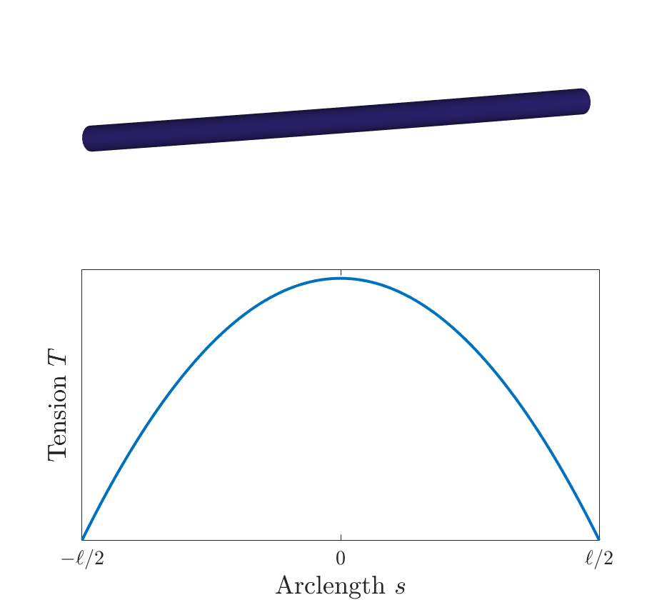
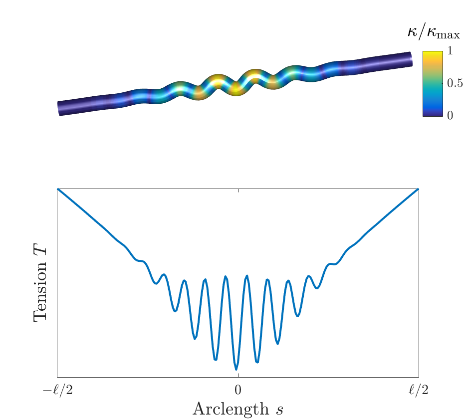
When the fiber is in a fully straight state (left panel of Fig. 1), one can assume that the tangent vector is constant, i.e. $\partial_{s}\mathbf{X}(s,t)=\mathbf{p}(t)$ at all values of $s$. As shown in [28], its direction $\mathbf{p}$ is then a solution of Jeffery’s equation for straight inertialess ellipsoidal rods

$$\frac{\mathrm{d}}{\mathrm{d}t}\mathbf{p}=\mathbb{A}\,\mathbf{p}-\dot{\gamma}\,\mathbf{p},\quad\mbox{with}\quad\dot{\gamma}(t)=\mathbf{p}^{\mathsf{T}}\mathbb{A}(t)\,\mathbf{p}.$$ (4)

The orientation $\mathbf{p}$ is sheared and rotated by the velocity gradient tensor $\mathbb{A}$, and the stretching/compression component given by $\dot{\gamma}$ is removed in order to fulfill the constraint $|\mathbf{p}|=1$. The corresponding term in the right-hand side of (4) indeed originates from the tension in the slender-body equation (1). The later is obtained by from (2) with $\partial_{s}\mathbf{X}=\mathbf{p}$, leading to

$$T(s,t)=-\frac{\mu}{4}\,\dot{\gamma}(t)\left(s^{2}-\frac{\ell^{2}}{4}\right),$$ (5)

meaning that the tension is maximal in the middle of the fiber and follows a parabolic shape with the arc-length coordinate $s$ (see left panel of Fig. 1). When the fiber is strongly compressed ($\dot{\gamma}<0$), the straight configuration might become unstable, leading to buckling (see right panel of Fig. 1). In that case, the tension can display several local extrema (this will be discussed later in Section 4.1).

In turbulence, fibers are most of the time in a straight state and very rarely buckle [25]. It was shown there that the buckling instability develops when the instantaneous value of $\dot{\gamma}$ takes large negative values. Besides, velocity gradients in turbulent flows can experience arbitrarily large fluctuations. This impacts the dynamics of the fiber, and in particular the transition rates between the straight and the buckled configurations. Explicitly, the fibers behave as stiff rods in calm regions, and fibers bend/stretch more frequently in very fluctuating regions.

Large turbulent fluctuations may then initiate a breakup process. Indeed, strong stretching and compression by the flow produces large values of the tension and curvature, respectively. As anticipated, two mechanisms can then initiate a fragmentation: tensile failure when the fiber breaks because the local tension is too high, and flexural failure when the fiber breaks due its curvature being too large. Large positive values of the tension leading to tensile failure are attained when the fiber is in a fully straight configuration and experiences a strong shear from the flow, as shown in the left-hand side of Fig. 1. In this configuration the bending energy is zero, thus the tension balance the stretching due to velocity gradients. The solution of the tension is then a parabola, where the maximum is attained in the middle of the fiber — as transpires from Eq. (5).

Conversely, as is illustrated on the top panel in the right side of Fig. 1, the curvature becomes very large during buckling. Such large values of the curvature could lead to fragmentation through flexural failure. These instabilities are typically dominated by a single mode with symmetric properties. Such modes depends on the flexibility of the fiber and on the magnitude of the compression by the flow. Depending on which of these two mechanisms is predominant, the fibers might break at different locations. This could imply very different evolutions of the distribution evolution of the fiber size distribution [30].

3 Fragmentation through tensile failure

We here start by investigating fragmentation due to large values of the tension. This occurs when the maximal tension along the fiber is larger than a critical value $T^{\star}$ that depends on its material properties. To estimate the contribution of this mechanism to the fragmentation process, we need to study both the rate $\lambda_{\mathrm{T}}(T^{\star})$ at which a large tension is attained and the location where the maximum is located on the fiber.

Large tensions are reached when the fiber experiences a strong stretching along its main axis and is thus generally in a fully straight state. In that case, we have seen in the previous section, c.f. Eq. (5), that the tension is a concave parabola with its maximum

$$T_{\mathrm{max}}=\frac{\mu\,\dot{\gamma}\,\ell^{2}}{16}$$ (6)

reached at the middle of the fiber. As a consequence, a tensile failure will always break short fibers in two equal pieces, giving a trivial daughter distribution. It should be noted here that this is true for fibers without molecular defects (i.e. $T^{\star}$ is constant along the fiber length).

Another consequence is that tensile failure occurs when the stretching rate along the fiber exceeds a critical value, namely $\dot{\gamma}>16\,T^{\star}/(\mu\ell^{2})$, and thus when the velocity gradient reaches strong positive values. Turbulent gradients along Lagrangian path are known to display very sharp fluctuations and oscillations. This implies that the rate at which a large value of $\dot{\gamma}$ is exceeded, is approximately proportional to the probability distribution at this value, so that

$$\lambda_{\mathrm{T}}(T^{\star})\propto\mathrm{Pr}\,\left(\dot{\gamma}>16\,T^{\star}/(\mu\ell^{2})\right).$$ (7)

The right-hand side involves the distribution of $\dot{\gamma}$ and thus that of fluid velocity gradients. In large-Reynolds-number turbulence, this distribution is fairly approximated by a log-normal with far tails which are actually closer to a stretched exponential with an exponent $\approx 1/2$ — see, e.g., [33, 32, 31, 34]). These two behaviours are confirmed in our numerical simulations. The inset of Fig. 2 shows the probability density function of the stretching rate $\dot{\gamma}$. Its behaviour at positive values is well represented by a log-normal distribution when $\dot{\gamma}$ is of the order of $\tau_{\eta}^{-1}$ with a far tail at $\dot{\gamma}\gg\tau_{\eta}^{-1}$ that rather approach a stretched exponential behaviour. As stressed in [35], the coefficients used in fits have a non-trivial dependence upon the Reynolds number. From now on, we focus on the case $R_{\lambda}=731$, as chosen in our simulation. We will come back to this dependence in the conclusions.

Figure 2: Tensile fragmentation rate $\lambda_{\mathrm{T}}$ as a function of the critical tension $T^{\star}$ for various values of the non-dimensional flexibility $\mathcal{F}$. The rate has been non-dimensionalised by $\tau_{\eta}^{-1}$ while the $x$ axis displays $\tau_{\eta}\,T^{\star}/(\mu\ell^{2})$. The solid line is the stretched-exponential fit (8) with $\lambda_{0}=14\,/\tau_{\eta}$, $c=34$ and $\tau\approx\tau_{\eta}$. The dashed line is the log-normal fit (9) with $\lambda_{0}^{\prime}=0.13/\tau_{\eta}$, $c^{\prime}=1.12$ and $\tau=102\,\tau_{\eta}$. Inset: Probability density function (PDF) of the stretching rate $\dot{\gamma}$ at positive values (blue bold solid line), together with a stretched exponential fit (black thin line) and a log-normal fit (dashed line).

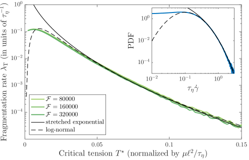
These considerations suggest to use these two possibles forms to fit the tensile fragmentation rate $\lambda_{\mathrm{T}}$ as a function of the physical parameters of the fiber. When $T^{\star}/(\mu\ell^{2})\gg\tau_{\eta}^{-1}$, a stretched-exponential form is expected to be more relevant, so that

$$\lambda_{\mathrm{T}}(T^{\star})\approx\lambda_{0}\,\exp\left[-c\,\left(\frac{\tau_{\eta}\,T^{\star}}{\mu\ell^{2}}\right)^{1/2}\right],$$ (8)

with fitting parameters a frequency, $\lambda_{0}$, and a dimensionless constant $c$. As can be seen in Fig. 2, such a formula gives indeed a good approximation to numerical calculations of the tensile fragmentation rates.

At $T^{\star}/(\mu\ell^{2})\sim\tau_{\eta}^{-1}$, as can be seen in Fig. 2, the tensile fragmentation rate behaves as a log-normal, namely

$$\lambda_{\mathrm{T}}(T^{\star})\approx\lambda_{0}^{\prime}\,\exp\left[-c^{\prime}\,\left(\log\frac{\tau\,T^{\star}}{\mu\ell^{2}}\right)^{2}\right],$$ (9)

where $c^{\prime}$ is a dimensionless fitting constant, and $\lambda_{0}^{\prime}$ and $\tau$ are fitting parameters with dimensions of a frequency and a time, respectively. The values of these parameters reported in the caption suggest that, while $\lambda_{0}^{\prime}$ is of the order of the Kolmogorov timescale $\tau_{\eta}$, the time $\tau$ is one hundred times larger. This can be explained by the fact that $T_{\mathrm{max}}(\mu\ell^{2})\sim\dot{\gamma}/16$ and in turn, as seen in [25], typical values of $\dot{\gamma}$ are of the order of $0.1/\tau_{\eta}$ leading to a factor of the order of 100.

To summarise this section, let us stress that tensile failure is here entirely prescribed by the (intermittent) statistics of the velocity gradients. This is a stylized feature of our approach, and provides a simplified framework to study fragmentation. Note that this assumption holds true only for small fibers. When considering fibers larger than the Kolmogorov length scale, the velocity gradient will not be uniform along the fiber. This implies in particular that the fiber could be locally stretched and compressed at the same time and breaks in pieces of arbitrary sizes.

Also, it is important to notice that reaching large values of the tension requires $\dot{\gamma}$ to locally exceed a critical value that is $\propto\ell^{-2}$. Tensile failure thus becomes rarer and rarer when fibers become smaller. In addition, the daughter population is typically centered over the half of the mother size. This implies that a fragmentation process involving only tensile failure cannot efficiently lead to the fast formation of small-size fragments. As we will see in the next section, this strongly differs when flexural failure is involved. In that case, many small segments can be created during a single event.

4 Fragmentation through flexural failure

Conversely to tensile failure, flexural failure displays a much more complicated behaviour. Such breakups happen when the fiber is bent and, more precisely, when the curvature becomes larger than a given threshold. Then, there exists a location $s$ along the fiber such that, at the breakup time $t^{\star}$, one has $|\partial_{s}^{2}\mathbf{X}(s,t^{\star})|\geq\kappa^{\star}$. Clearly, as the curvature is continuous with respect to arc-length and time, such a breakup occurs at the first time when the maximum of curvature $\kappa_{\mathrm{max}}=\max_{s}|\partial_{s}^{2}\mathbf{X}|$ exceeds $\kappa^{\star}$. As anticipated in §2, these events happen when the fiber undergo a buckling. Such an instability occurs when the instantaneous value of the stretching rate $\dot{\gamma}$ defined in Eq. (4) becomes large negative (compression). The upper-left panel of Fig. 3 shows the time evolution of the fiber’s maximal curvature along a Lagrangian trajectory for different values of $\mathcal{F}$. It can be seen that buckling events, for which $\kappa_{\mathrm{max}}\neq 0$, are very sparse and intermittent. Such events are separated by long periods, which can be of the order of the large-eddy turnover time, during which the fiber is fully straight, up to numerical precision. It is shown in Ref. [25] that in turbulence, the rate at which buckling appears is similar to an activation process. More precisely, it was found that the fiber buckles when its instantaneous flexibility $\mathcal{F}_{\rm loc}(t)=\tau_{\eta}\,|\dot{\gamma}(t)|\,\mathcal{F}$ becomes larger than a critical value $\mathcal{F}^{\star}$, provided that $\dot{\gamma}(t)<0$. This leads to estimate the buckling rate as

$$\lambda_{\mathrm{Buckl}}\propto\mathrm{Pr}\,\left(\dot{\gamma}<-\mathcal{F}^{\star}/(\tau_{\eta}\,\mathcal{F})\right).$$ (10)

As in the case of tensile failure rates, the distribution of the stretching rate $\dot{\gamma}$ can be approximated either by a log-normal or by a stretched exponential, leading to approximations of the above formula. We expect the rate of flexural failure to be upper bounded by this buckling rate.

Figure 3: Left panel: Time evolution of the maximal curvature $\kappa_{\mathrm{max}}$ along a single turbulent tracer trajectory but for three different values of the non-dimensional flexibility $\mathcal{F}$. The upper part shows the full trajectory, while the lower is a semilogarithmic time zoom on the buckling event occurring at time $t\approx 337\,\tau_{\eta}$. Right panel: Rates at which the maximal curvature exceeds given values $\kappa^{\star}$ (as labelled) as a function of the non-dimensional flexibility. Each dataset is fitted by both a stretched exponential (solide curves) and by a log-normal (dashed curves).

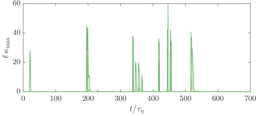
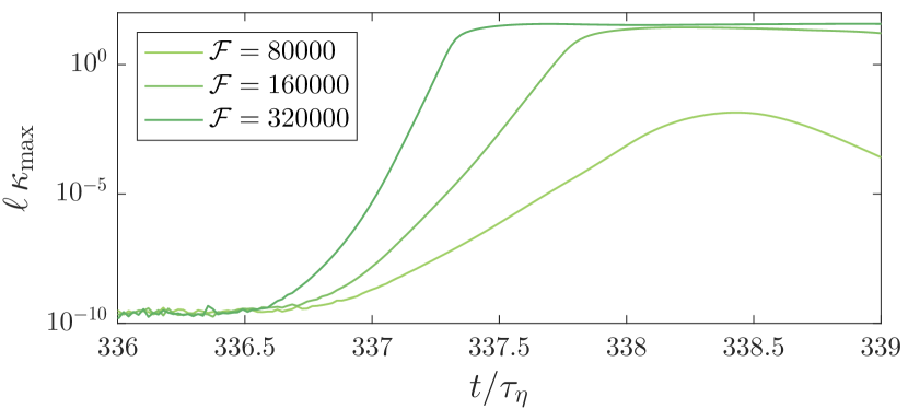
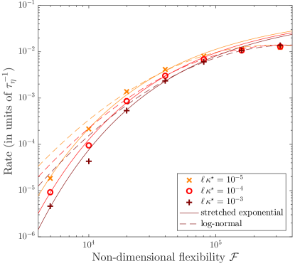
However, for breakup to occur, we additionally require that the maximum curvature exceeds $\kappa^{\star}$. The corresponding rates are shown on the right-hand panel of Fig. 3 as a function of the non-dimensional flexibility $\mathcal{F}$ and for various values of the threshold $\kappa^{\star}$. Log-normal and stretched exponential functional forms give good approximations with fitting parameters that depend on $\kappa^{\star}$. Understanding this dependence requires investigating more closely the development of the instability. The lower-left panel of Fig. 3 shows the time growth of the maximum of curvature during one of these events for various values of the non-dimensional flexibility. One observes that the increase is approximately exponential with a rate that depends on $\mathcal{F}$. Small values of $\kappa^{\star}$ are reached during the instability growth and it is thus needed to characterise further this regime in order to quantify how this affect rates. The development of the buckling instability is furthermore of importance as flexural failure will actually not happen when the threshold is exceeded but rather when it is for the first time. At difference with tension that has fast fluctuations, the curvature has an on-off behaviour. As can be seen on the lower-left panel of Fig. 3, the growth of $\kappa_{\mathrm{max}}$ can be followed by a period during which it remains at finite values for quite some time. This indicates that the rates shown on the right-hand panel of Fig. 3 are actually overestimating the actual flexural failure rates. In the following, we provide more accurate estimates.

4.1 Linear analysis and relevance to turbulent flows

The buckling instability occurs when the fiber, initially in a straight configuration $\partial_{s}\mathbf{X}\equiv\mathbf{p}$, experiences a strong compression by the flow. This is likely to happen when the flow locally displays a violent shear, so that the rodlike fiber undergoes what is known as a Jeffery orbit [29]: In that case, the rod rotates periodically and is not aligned with the flow. During such an orbit, the fiber alternatively experience stretching and compression along its main axis, giving it the opportunity to buckle. Performing a linear stability analysis for such orbits is however complex. Indeed, upon buckling, the initially straight fiber picks a specific trajectory among an infinite family. The selected trajectory depends on the initial perturbation and is very sensitive to fine sub-leading details, such as thermal noise [36], fiber or fluid inertia [37, 38], or, as in our turbulent settings, the fact that the flow is not a pure shear.

As we will see in the sequel, a simplified linear stability analysis already fairly describes buckling events, meaning that we can avoid delving into the complicated context of Jeffery orbits. Let us consider that the fiber experiences a time-constant compression $\dot{\gamma}=\mathbf{p}^{\mathsf{T}}\mathbb{A}\,\mathbf{p}<0$ along its direction. The base solution $\mathbf{p}(t)$ describes a rod-like solution to the slender body equation (1). We introduce a perturbed solution as $\mathbf{X}(s,t)=\bar{\mathbf{X}}(t)+s\,\mathbf{p}(t)+\bm{\chi}(s,t)$, where $\bar{\mathbf{X}}(t)$ is the average position of the fiber center of mass and the perturbation $\bm{\chi}$ is of small amplitude (i.e. $|\bm{\chi}|\ll\ell$). For buckling, we are interested in perturbations that grow perpendicularly to the fiber direction. The two transverse components of $\bm{\chi}$ are decoupled and evolve as (see, e.g., [18])

$$\frac{1}{|\dot{\gamma}|}\,\partial_{t}\chi=\chi+s\,\partial_{s}\chi+\frac{1}{4}\left(s^{2}-\frac{\ell^{2}}{4}\right)\partial_{s}^{2}\chi-\frac{E}{\mu\,|\dot{\gamma}|}\,\partial_{s}^{4}\chi,$$ (11)

with the free-end boundary conditions $\partial_{s}^{2}\chi=0$ and $\partial_{s}^{3}\chi=0$ at $s=\pm\ell/2$. This linear equation admits solutions of the form $\chi(s,t)=e^{\rho\,t}\hat{\chi}(s)$, where $\hat{\chi}$ is the eigenfunction of the right-hand side of (11) associated to the eigenvalue $\rho$. Once time is rescaled by $\dot{\gamma}^{-1}$ and arc-length by $\ell$, this eigenvalue problem depends on a unique non-dimensional parameter $\mathcal{F}_{\mathrm{loc}}=\mu\,|\dot{\gamma}|\,\ell^{4}/E$, which measures the ratio between the fluid compression and the elastic force. Because of the presence of non-constant coefficients, there is no straightforward way to obtain the full spectrum of eigenmodes as a function of the dimensionless flexibility $\mathcal{F}_{\mathrm{loc}}$. Still, there are two trivial solutions given by $\rho/\dot{\gamma}=1$ with $\hat{\chi}=\mathrm{const}$ and $\rho/\dot{\gamma}=2$ with $\hat{\chi}=a\,s$ and $a$ constant. For these two unstable modes, the fiber remains straight and does not buckle. To access more complicated configurations, we rely on integrating numerically equation (11).

Figure 4: Left panel: Thirty largest eigenvalues associated to the linear evolution (11) as a function of $\mathcal{F}_{\mathrm{loc}}$. The two horizontal lines at $\rho=\dot{\gamma}$ and $\rho=2\dot{\gamma}$ show the two unstable straight modes. The three vertical lines at $\mathcal{F}_{\mathrm{loc}}=\mathcal{F}^{\star}_{1}$, $\mathcal{F}^{\star}_{2}$, and $\mathcal{F}^{\star}_{3}$ are bifurcations above which the most unstable non-straight mode is $n=1$, $2$, and $3$, respectively. The dashed line represents the asymptotic behaviour $\rho/\dot{\gamma}\simeq\mathcal{F}_{\mathrm{loc}}/1024$ reached at large values. Right panel: illustrations of the fiber geometric state in eigenmodes of various orders $n$.

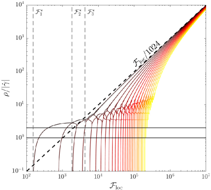
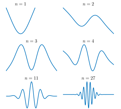
The left panel of Fig. 4 represents the thirty most unstable eigenvalues as a function of the non-dimensional flexibility. A first non-straight mode becomes unstable when $\mathcal{F}_{\mathrm{loc}}>\mathcal{F}_{1}^{\star}\approx 153$. This threshold is in agreement with [18]. This first growing mode, labelled as $n=1$, is shown in the right-hand panel of the figure. When $\mathcal{F}_{\mathrm{loc}}$ increases, there is a sequence of bifurcations with a change of the most unstable eigenfunction. We label these modes with the number $n$ of extrema that $\hat{\chi}$ contains (see right-hand panel). The first bifurcation is between order $n=1$ and $n=2$, which occurs at $\mathcal{F}_{\mathrm{loc}}=\mathcal{F}_{2}^{\star}\approx 1840$. When $\mathcal{F}_{\mathrm{loc}}$ further increases, the most unstable modes are of higher order $n$. It also appears from the right panel of the figure that the amplitude of fluctuations decreases very fast as the arc-length coordinate $s$ gets further from the fiber center. One finally observes that when $\mathcal{F}_{\mathrm{loc}}\to\infty$, the most unstable eigenvalues grow as $\rho/\dot{\gamma}\propto\mathcal{F}_{\mathrm{loc}}$.

In this asymptotics of large dimensionless flexibility, the small parameter $\mathcal{F}_{\mathrm{loc}}^{-1}$ multiplies the highest-order derivatives. This indicates that the limit is singular but could actually be tackled using a WKB perturbative approach (see, e.g., [39]). The WKB method suggests writing the solution as the exponential of an asymptotic series expansion

$$\hat{\chi}(s)\sim\exp\left(\frac{1}{\varepsilon}\sum_{p\geq 0}\varepsilon^{p}\varphi_{p}(s)\right),$$ (12)

where $\varepsilon=\mathcal{F}_{\mathrm{loc}}^{-\delta}$ is a small parameter and $\varphi_{p}(s)$ are terms in the expansion. The exponent $\delta>0$ is obtained by substituting the expansion (12) in (11) and balancing the leading-order terms. Far from the fiber’s ends, one has

$$\frac{\rho}{|\dot{\gamma}|}=\frac{1}{4\,\varepsilon^{2}}\left(s^{\prime 2}-\frac{1}{4}\right)\left(\partial_{s^{\prime}}\varphi_{0}\right)^{2}-\frac{1}{\mathcal{F}_{\mathrm{loc}}\,\varepsilon^{4}}\,\left(\partial_{s^{\prime}}\varphi_{0}\right)^{4},$$ (13)

with $s^{\prime}=s/\ell$. This gives $\varepsilon=\mathcal{F}_{\mathrm{loc}}^{-1/2}$ and $\rho/|\dot{\gamma}|\sim\mathcal{F}_{\mathrm{loc}}$, meaning that $\delta=1/2$ and confirming the observed linear behaviour of the eigenvalues in the asymptotics of $\mathcal{F}_{\mathrm{loc}}\to\infty$. Besides, when $\mathcal{F}_{\mathrm{loc}}$ increases, the order $n$ of the dominant mode becomes larger and the eigenfunction gets more localised at $|s^{\prime}|\ll 1$. This suggests expressing the dominant term as $\varphi_{0}(s^{\prime})=a_{0}+a_{1}\,s^{\prime}+a_{2}\,s^{\prime 2}+a_{3}\,s^{\prime 3}+\cdots$. Now, using this expansion in (13) and balancing equal powers of $s^{\prime}$, one obtains to leading order

$$\frac{\rho}{|\dot{\gamma}|}=-\frac{\mathcal{F}_{\mathrm{loc}}}{16}\,a_{1}^{2}-\mathcal{F}_{\mathrm{loc}}\,a_{1}^{4},\quad\mbox{so that }\ a_{1}^{2}=-\frac{1}{32}\pm\sqrt{\frac{1}{1024}-\frac{\rho}{|\dot{\gamma}|\,\mathcal{F}_{\mathrm{loc}}}}.$$ (14)

This leading term contributes an exponential behaviour $\propto\exp(\pm\sqrt{\mathcal{F}_{\mathrm{loc}}}\,a_{1})$ at $s^{\prime}=\pm 1$ in the eigenfunction $\hat{\chi}$. When the real part of $b$ is non-zero, this term diverges as a function of $\mathcal{F}_{\mathrm{loc}}$ and this is incompatible with the imposed free-end boundary conditions. $a_{1}$ should thus be a pure imaginary number. This means that $a_{1}^{2}$ is real negative, and with (14), we get necessarily $\rho/\dot{\gamma}<\mathcal{F}_{\mathrm{loc}}/1024$, the maximal eigenvalue corresponding to the case when the bound is reached. This prediction gives the value $1/1024$ for the constant of the linear behaviour of $\rho$, in agreement with the measurements reported in Fig. 4. Note that for this specific eigenvalue, one obtains $a_{1}=\mathrm{i}/\sqrt{32}$ ($\mathrm{i}$ being the imaginary unit).

Moving on to higher-order terms, one can easily check that contributions of the order of $s^{\prime}$ vanish for the above value of $a_{1}$. As to the terms $\propto s^{\prime 2}$, they give

$$0=\frac{1}{4}a_{1}^{2}-\frac{1}{16}(4\,a_{2}^{2}+6\,a_{1}a_{3})-\left(24\,a_{1}^{2}a_{2}^{2}+12\,a_{1}^{3}a_{3}\right).$$ (15)

Using $a_{1}=\mathrm{i}/\sqrt{32}$, we get $a_{2}=-1/8$. This finally leads to writing $\varphi_{0}\approx a_{0}+\mathrm{i}\,s^{\prime}/\sqrt{32}-s^{\prime 2}/8$.

This asymptotic analysis suggest to write the eigenfunction of order $n$ as

$$\hat{\chi}(s)=\left\{\begin{array}[]{ll}\mathrm{e}^{-c\,(s/\ell)^{2}}\cos(2\pi\,k^{\star}\,s/\ell)&\mbox{for }n=2\,k^{\star}+1\mbox{ odd},\\ \mathrm{e}^{-c\,(s/\ell)^{2}}\sin(2\pi\,k^{\star}\,s/\ell)&\mbox{for }n=2\,k^{\star}\mbox{ even},\end{array}\right.$$ (16)

whose typical shape is represented on the left-hand side of Fig. 5. The above asymptotic analysis shows that the most unstable mode is characterised by an oscillating function with a wavelength $k^{\star}$ and a Gaussian envelope with a coefficient $c$. These two parameters are given by:

$$k^{\star}\simeq{\sqrt{\mathcal{F}_{\mathrm{loc}}}}/{(2\pi\sqrt{32})}\quad\mbox{and}\quad c\simeq{\sqrt{\mathcal{F}_{\mathrm{loc}}}}/{8}.$$ (17)

To estimate numerically $k^{\star}$ and $c$, we use the Fourier spectrum of the eigenfunction. It is defined as the squared modulus of the coefficients of the Fourier transform of $\hat{\chi}$. As illustrated on the right-hand side of Fig. 5, the spectrum of the asymptotic form (16) is a Gaussian function of $k$. The wavenumber $k^{\star}$ is approximated as the mean associated to this distribution, while the coefficient $c$ is deduced from its variance. We use this approach to measure $k^{\star}$ and $c$ as a function of $\mathcal{F}_{\mathrm{loc}}$ for the eigenfunctions obtained numerically from the integration of the linear system (11). The results are displayed as red solid curves on Fig. 6, together with the asymptotic predictions (17) displayed as black dashed curves. The good agreement between these curves confirm the relevance of the asymptotic analysis at large values of $\mathcal{F}_{\mathrm{loc}}$ that we consider here.

Figure 5: Left: Typical asymptotic shape of the eigenfunctions consisting of a fast oscillation with a Gaussian envelope. Right: Spectrum $E(k)=|\mathbb{F}[\hat{\chi}](k)|^{2}$ of the same function, where $\mathbb{F}[\hat{\chi}]$ designates the Fourier transform of $\hat{\chi}$. It is a Gaussian centered at $k=k^{\star}$ with variance $c/(2\pi^{2})$.

Figure 6: Numerical estimates of the wavenumber $k^{\star}$ (Left) and of the coefficient $c$ of the Gaussian envelope (Right) characterising the most unstable mode. Results are shown both for the numerical integration of the linearised dynamics (red solid curves) and for turbulent data (symbols associated to various $\mathcal{F}$, as labelled). The asymptotic predictions (17) are shown as black dashed curves.

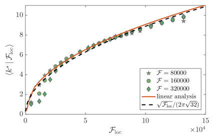
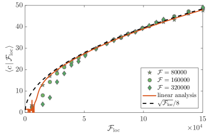
Following this linear analysis, we then perform the same kind of analysis to the case of fibers that follow turbulent trajectories. To capture the dawn of the instability, we track fibers whose curvature, after having almost relaxed to zero, grows again and exceeds a given threshold. We use the fiber’s shape at the instant of time when the threshold is first reached as an estimate of the growing mode. In such fluctuating settings, we make use of the instantaneous non-dimensional flexibility $\mathcal{F}_{\mathrm{loc}}=\tau_{\eta}|\dot{\gamma}|\,\mathcal{F}$. For each event, we measure $k^{\star}$ and $c$ from the Fourier spectrum of the fiber shape. We then compute their average value conditioned on the observed value of $\mathcal{F}_{\mathrm{loc}}$. The resulting estimates are shown as symbols on Fig. 6 for three different values of $\mathcal{F}$. Clearly, these measurements show that the linear analysis reported above is able to describe the growth of buckling modes in turbulent flows, assuming that the relevant parameter is given by the instantaneous value of the non-dimensional flexibility.

4.2 Estimates for flexural fragmentation rates in turbulence

We now apply the above considerations to determine both the rate at which flexural failure occurs and the resulting daughter size distribution upon fragmentation. We assume that the fibers are brittle, so that they break as soon as their curvature exceeds a critical value $\kappa^{\star}$, which is relatively small. Because of that, breakup happens while the fiber is still at the beginning of a buckling event that can be described within the linear approximation. We moreover assume that the instability growth is given by eigenvalues and eigenfunctions that are properly described by the large-flexibility asymptotics of the previous subsection.

Fragmentation rate

The rate at which flexural failure occurs is the rate at which the maximal curvature along a fiber exceeds for the first time the critical value $\kappa^{\star}$. A first condition for this to happen is to have the fiber developing a buckling: this requires $\mathcal{F}_{\mathrm{loc}}=\tau_{\eta}\,|\dot{\gamma}|\,\mathcal{F}$ becoming larger than a critical value $\mathcal{F}^{\star}$ at time $t_{0}$, which marks the beginning of the event. After that, the instability grows exponentially with a rate $\rho\simeq|\dot{\gamma}|\,\mathcal{F}_{\mathrm{loc}}/1024$. The maximal curvature also follows this growth, so that

$$\kappa_{\mathrm{max}}(t)\simeq\kappa_{\mathrm{max}}(t_{0})\,\exp\left[\frac{\tau_{\eta}\,|\dot{\gamma}|^{2}\,\mathcal{F}}{1024}\,(t-t_{0})\right].$$ (18)

Of course, without an initial curvature nothing would happen. It is indeed required to have initially a small deviation to the base state for the instability to develop. In physical situations, several effects give such perturbations, including thermal noise, material inhomogeneities along the fibers, a small extensibility, the fluid flow modifications due to the fiber, and more importantly, the sub-leading turbulent fluctuations that are neglected when we assume that the fiber samples a space-independent fluid velocity gradient. Such effects are clearly not in the model we use. Still, in our simulations, the instability is triggered by a small numerical noise that comes either from the accuracy of the method, from roundoff errors, or from the penalty approach that is used to enforce inextensibility. This error is visible in the lower-left panel of Fig. 3 where, before the buckling starts, one has $\kappa_{\mathrm{max}}\approx\kappa_{0}\approx 2\times 10^{-10}\,\ell^{-1}$.

No matter how small they are, arbitrary values of curvature are not necessarily reached by all buckling events. For instance, during the specific event shown in the lower-left panel of Fig. 3, the maximal curvature barely reaches $\kappa_{\mathrm{max}}=10^{-2}\,\ell^{-1}$ in the case of the fiber with the smallest flexibility. The growth rate is there too small or, equivalently, compression does not last long enough. During this very event, the two other more flexible fibers reach much larger curvatures and saturate at $\kappa_{\mathrm{max}}\approx 30\ell^{-1}$. These distinct behaviours originate from large differences in the instability growth rates. The time during which the fiber is compressed is completely determined, either by the fluid flow through the Lagrangian persistence time of velocity gradients, or by the evolution of the base orientation $\mathbf{p}(t)$, which for instance perform a Jeffery orbit and tumbles. In both cases, the relevant timescale during which the fiber is compressed is of the order of $|\dot{\gamma}|^{-1}$.

A necessary condition for the fiber to break is thus that it reaches curvatures larger than $\kappa^{\star}$ on a time smaller than the compression duration $\simeq\alpha\,|\dot{\gamma}|^{-1}$, where $\alpha$ is an order-unity constant. Using the exponential law (18), one should thus have

$$t-t_{0}\simeq\frac{1024}{\tau_{\eta}\,|\dot{\gamma}|^{2}\,\mathcal{F}}\,\log(\kappa^{\star}/\kappa_{0})<\alpha\,|\dot{\gamma}|^{-1}.$$ (19)

This leads to the following estimate for the rate at which flexural failure occurs

$$\lambda_{\mathrm{K}}(\kappa^{\star})\propto\mathrm{Pr}\,\left(\dot{\gamma}<-\left[(1024/\alpha)\,\log(\kappa^{\star}/\kappa_{0})\right]/(\tau_{\eta}\,\mathcal{F})\right).$$ (20)

This formula is similar to the buckling rate of Eq. (10) except that, this time, the critical non-dimensional flexibility depends on $\kappa^{\star}$. Also, it suggests that $\lambda_{\mathrm{K}}$ is simply a function of the dimensionless parameter $(1/\mathcal{F})\,\log(\kappa^{\star}/\kappa_{0})$, that can be fitted, as before, by either a stretched exponential or a log-normal.

Figure 7: Left: Complementary Cumulative Distribution Function (CDF) of the first time at which the fibers curvature hits a value $\kappa^{\star}=10^{-6}$, shown for various values of the flexibility, as labelled. (Time is here in units of $\tau_{\eta}$.) Right: Fragmentation rate $\lambda_{\mathrm{K}}$ as a function of the dimensionless parameter $(1/\mathcal{F})\,\log(\kappa^{\star}/\kappa_{0})$, with a reference curvature set to $\kappa_{0}=2\times 10^{-10}$. Symbols correspond to different values of $\kappa^{\star}$ and $\mathcal{F}$. The solid line is the stretched-exponential fit (21) with $\lambda_{0}=0.055\,\tau_{\eta}^{-1}$ and $c=160$. The dashed line is the log-normal fit (22) with $\lambda_{0}^{\prime}=0.06\,\tau_{\eta}^{-1}$, $c^{\prime}=0.11$, and $a^{\prime}=13.12$.

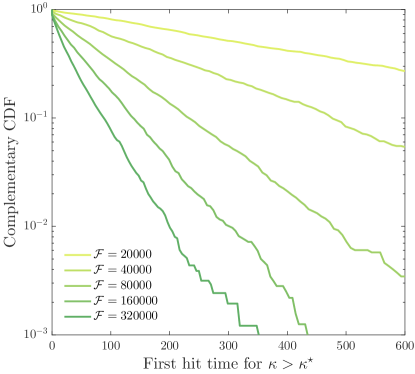
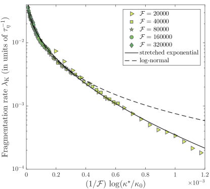
To test this prediction numerically, the main difficulty is to estimate this rate from finite-time simulations. Depending on the values of the fiber flexibility and of the critical curvature, the typical time needed for the curvature to become larger than $\kappa^{\star}$ can be longer than the simulation duration. Hence, to estimate this rate, we have rather measured the probability distribution of the first time at which $\kappa_{\mathrm{max}}$ hits $\kappa^{\star}$. The complementary cumulative distribution function is shown on the left panel of Fig. 7 for different flexibilities and a fixed value of the critical curvature. Clearly, one observes that the first-hit time follows an exponential law. Fitting such laws gives a straightforward way to estimate $\lambda_{\mathrm{K}}$ as a function of the two parameters $\mathcal{F}$ and $\kappa^{\star}$. The results are shown in the right panel of Fig. 7. One finds that when $\mathcal{F}$ is large-enough, all data indeed collapse when represented as a function of the non-dimensional parameter $(1/\mathcal{F})\,\log(\kappa^{\star}/\kappa_{0})$.

To propose fitting formulae for this rate, we rely on approximating the distribution of turbulent velocity gradients by either a stretched exponential or a log-normal law, as was done for tensile failure. In the first case, we write

$$\lambda_{\mathrm{K}}(\kappa^{\star})\approx\lambda_{0}\,\exp\left[-c\,\left(\frac{\log(\kappa^{\star}/\kappa_{0})}{\mathcal{F}}\right)^{1/2}\right],$$ (21)

with fitting parameters $\lambda_{0}$ (with the dimension of a frequency) and $c$ (dimensionless). As can be seen in the left-hand side of Fig. 7, this a formula gives a rather good approximation. As to the log-normal fit, it reads

$$\lambda_{\mathrm{K}}(\kappa^{\star})\approx\lambda_{0}^{\prime}\,\exp\left[-c^{\prime}\,\left[\log\left(\frac{\log(\kappa^{\star}/\kappa_{0})}{\mathcal{F}}\right)+a\right]^{2}\right],$$ (22)

where the fitting parameters are this time a frequency $\lambda_{0}^{\prime}$ and two dimensionless parameters $c^{\prime}$ and $a^{\prime}$. As for tension, the log-normal fit does not describe well data associated to the tail of the distribution, that is small values of $\mathcal{F}$ or, equivalently, large values of $\kappa^{\star}$. These two fits provide estimates of the rate at which flexural failure occurs as a function of all physical parameters, including the fiber length, aspect ratio, Young modulus, the fluid velocity and mass density that enter the definition of the non-dimensional flexibility $\mathcal{F}$ given in Eq. (3).

Daughter size distribution

We next turn our attention to understand the resulting sizes of the fragments obtained due to flexural failure during buckling. Up to now, by focusing on the flexural failure rate, we have addressed only a single (the first) breakup event. Because the fiber is curved according to a given buckling mode of order $n$, the location where breakup occurs clearly depends on $n$. When $n$ is is odd, the breakup occurs at the center of the fiber, which breaks in two equal pieces. When $n$ is even, the two resulting fragments have approximately sizes $\ell\times(n/2)/(n+1)$ and $\ell\times(n/2+1)/(n+1)$. Actually, this primary breakup is sometimes followed by successive fragmentations. We indeed find that, because of the continuing compression by the flow, the unstable mode keeps on bending the small secondary pieces, so that their curvature still grows and can reach again the critical value. This is illustrated for a specific buckling event in Fig. 8 where we have implemented in the numerical simulation the breakup process and the follow-up of resulting fragments. In this case, the instability triggers the growth of a mode of order $n=14$ (top-left panel of Fig. 8). A first breakup occurs at $s\approx-0.02\,\ell$, but the resulting fragments undergo successive fragmentations. This process finally leads to the formation of eight pieces. In this daughter distribution, six fragments have sizes of the order of $\ell/(n+1)\approx 0.07\,\ell$, the two remaining being associated to the ends of the original fiber (bottom-left panel). As can be followed on the right-hand panel, the locations where new breakups occur follow the structures of the initial bending. Note that the full process occurs on timescales of the order of $\tau_{\eta}$, confirming that this corresponds to a single buckling event.

Figure 8: Evolution of a fiber during fragmentation. The top-left panel shows the growing mode by displaying, at the time of the first breakup, the fiber’s curvature as a function of the arc-length $s$. The bottom-left panel represents the time evolution of the size distribution (time growing from top to down); Each horizontal plain line is a breakup event and segments correspond to fiber fragments. The right-hand side shows three instantanenous configurations of the fragments at time $t_{1}$, $t_{2}$ and $t_{3}$. Colors code the values of curvature (from zero in dark blue to $\kappa^{\star}$ in yellow). Note that on this pseudo 3D representation, the arc-length $s$ runs from right to left.

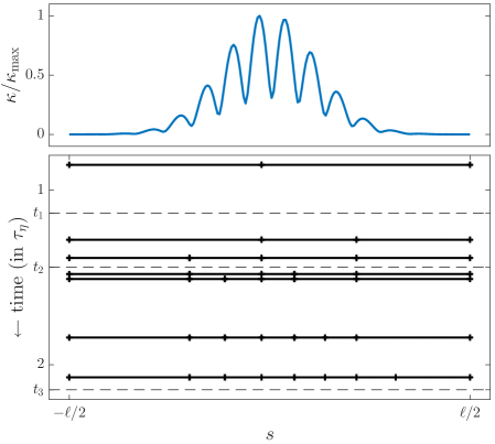
A single buckling event can hence lead to the creation of several small pieces, depending on which wavenumber is excited. The selection of the most unstable mode depends on the local value of the non-dimensional flexibility $\mathcal{F}_{\mathrm{loc}}=\tau_{\eta}\,|\dot{\gamma}|\,\mathcal{F}$, which fluctuates with $\dot{\gamma}$. Following the results of previous section, we expect for a given value of $\mathcal{F}_{\mathrm{loc}}$ that the most unstable mode is of order $n\simeq 2k^{\star}\simeq\sqrt{\mathcal{F}_{\mathrm{loc}}}/(\pi\sqrt{32})$. In that case, the daughter distribution will be peaked at $\ell^{\prime}=\ell/(n+1)\simeq\pi\sqrt{32}\,\ell/\sqrt{\mathcal{F}_{\mathrm{loc}}}$. Assuming that each buckling event leads to break the fiber in $(n+1)$ fragments of equal size $\ell^{\prime}$, we can draw an approximation for the daughter size distribution. Hence, the probability that a fiber of length $\ell$ breaks in $\ell/\ell^{\prime}$ fragments of size $\ell^{\prime}$ reads

$$\mathrm{Pr}(\ell\rightarrow\ell^{\prime})\propto\frac{\ell/\ell^{\prime}}{\tau_{\eta}\,\mathcal{F}}\,\ p_{\dot{\gamma}}\!\left(-32\,\pi^{2}(\ell/\ell^{\prime})^{2}/(\tau_{\eta}\,\mathcal{F})\right),$$ (23)

where $p_{\dot{\gamma}}(\cdot)$ denotes the probability density function of the stretching rate $\dot{\gamma}$. Assuming as previously that the later follows a stretched-exponential law, one obtains

$$\mathrm{Pr}(\ell\rightarrow\ell^{\prime})\propto\frac{\ell/\ell^{\prime}}{\mathcal{F}}\,\mathrm{e}^{-c\,(\ell/\ell^{\prime})/\sqrt{\mathcal{F}}}$$ (24)

where $c$ is a positive constant. This particularly simple form suggests that the creation of small-length fragments follows an activation-like distribution. In practical terms, this implies that fragment sizes below $c\ell/\sqrt{F}$ are statistically irrelevant and almost never observed. An equivalent form can be written for log-normal statistics of $\dot{\gamma}$, namely

$$\mathrm{Pr}(\ell\rightarrow\ell^{\prime})\propto\frac{\ell/\ell^{\prime}}{\mathcal{F}}\,\mathrm{e}^{-c^{\prime}\,\left[\log\left((\ell/\ell^{\prime})^{2}/\mathcal{F}\right)+a^{\prime}\right]^{2}}$$ (25)

with $a^{\prime}$ and $c^{\prime}$ constants. This second leads to the same qualitative considerations as above.

Figure 9: Histogram of the length $\ell^{\prime}$ of fragments stemming from the first fragmentation event encountered by $2000$ fibers with initial length $\ell$ and a flexibility $\mathcal{F}=320000$.

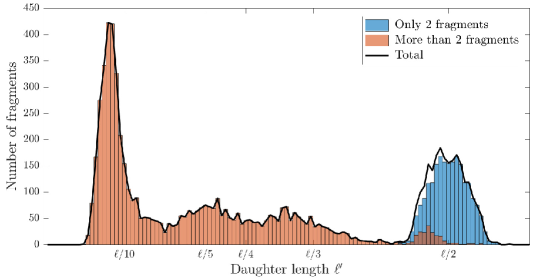
Finally, to illustrate the complexity of this process, we show in Fig. 9, the fiber length distribution of fibers after the first fragmentation series. All fibers have initially the same length $\ell$ and the same non-dimensional flexibility $\mathcal{F}=32000$. The simulation is done for a specific value of the critical curvature ($\kappa^{\star}=10^{-6}\ell^{-1}$), above which these fibers break. A fragmentation series is defined as the set of breakups occurring during the same buckling event, that is in a time lag going from the initial development of the buckling instability to the time when all fragments have relaxed to a fully straight configuration. The resulting distribution is clearly multi-modal. It develops a peak at sizes $\ell^{\prime}$ of the order of $\ell/2$, corresponding to fibers that broke only once during this series. Such events represent approximately one half of the fragmentations. Another marked peak is present at $\ell^{\prime}\approx\ell/12$. This other maximum is an artefact of the representation, as smaller are the segment, more numerous they are. Clearly, the number of fragments sharply tends to zero when their size becomes very small. Finally, the distribution displays finite values at intermediate sizes, contributing a significative probability of obtaining fragments of sizes $\ell/3$, $\ell/4$, $\ell/5$, etc.

5 Conclusions and perspectives

We have studied the fragmentation processes undergone by small, inextensible, inertialess fibers in turbulent flow, focusing on tensile and flexural failures. In both cases, we have shown that breakup occurs when the fiber runs into a flow region of high strain, where it is either stretched above internal cohesive forces or compressed, buckles and fractures under excessive bending. By assuming an idealised description for internal fragmentation processes, we found that the fragmentation rates can be expressed through the distribution of turbulent stretching rates. Using standard functional approximations for such probability laws, we proposed fits for both the tensile failure and the flexural failure rates that are calibrated and validated against the results of direct numerical simulations in a high-Reynolds-number flow. Our analysis emphasises the central role played by the fibers non-dimensional flexibility in understanding how frequently fragmentation occurs.

Besides rates, we reported results on daughter size distributions upon fragmentation. Tensile failure always occurs when the fiber is stretched by the flow and thus has a fully straight configuration. The tension is then maximal at its center, so that this type of breakup always produces two fragments with equal sizes. We found that the situation is more intricate in the case of flexural failure. Fragmentation occurs when the fiber develops a buckling instability and the resulting breakup process produces a size distribution that depends on the details of the most unstable buckling mode. By performing a linear stability analysis, we provided estimates of this size distribution that depend on the instantaneous fluid strain experienced by the fiber. This approach indicates that the number of fragments produced upon breakup becomes larger when the fibers experiences more violent compressions. Our analysis builds upon the results of Vandenberghe & Villermaux [13] on how buckling affects the fragmentation of elastic slender bodies. Specifically, they show the existence of an additional effect in the fragmentation process: the propagation of elastic waves after a first breakup. The released energy is able to increase further the curvature in the newly separated parts of the fiber, possibly leading to successive secondary breakups and to the formation of many small-size fragments. In our work, we unveil another, possibly complementary mechanism where the smaller-size fragments appear as fingerprints of the initial most-unstable growing mode.

An appealing prospective to our work concerns the Reynolds-number dependence of fragmentation rates and processes. While our numerics limited themselves to a single level of turbulence, our analysis can be easily extended to encompass intermittent descriptions of turbulent statistics. At a qualitative level, one expects more violent fluctuations as the Reynolds number increases. This implies that the rare events leading to the production of many small fragments should have an increasing statistical relevance. At a quantitative level, one can for instance apply the recent work of Buaria et al. [35] who carefully investigated the Reynolds-number dependence of the probability distributions of velocity gradients. Their findings can be straightforwardly used in our approach to write an explicit Reynolds-number dependence of the fragmentation rates and associated daughter size distributions.

Finally, it is important to stress again that, in this work, we have oversimplified the microscopical breakup processes by considering that the fibers material is brittle and that fibers are free of any molecular defects. In most realistic settings, the threshold value for each breakup mechanism may vary along the fiber length while plastic effect cannot be neglected, meaning that flexural failure may occur at locations that have been bended several times in the fiber’s history. Even if they involve an extra parametrisation, such effects can be easily implemented and investigated numerically (see, e.g., [40]). We expect in particular interesting impacts of the non-trivial time distribution of violent fluctuations. The turbulent fluid strain that is experienced by a fiber along its Lagrangian trajectory is typically very intermittent in time, so that buckling events are strongly correlated among each other. Nevertheless, generalising to such settings the analysis that has been developed here represents a real challenge. The strongest bending is indeed expected to occur when the buckling instability has saturated, questioning in that case the relevance of the linear analysis.

References

- [1] Beysens D, Campi X, Pefferkorn E. 1995. Fragmentation Phenomena. Singapore: World Scientific.
- [2] Hüfner J, Mukhopadhyay D. 1986. Fragmentation of nuclei, stones and asteroids. Phys. Lett. B 4, 373–376 (See doi.org/10.1016/0370-2693(86)90397-7)
- [3] Nagata S. 2000. Apoptotic DNA fragmentation. Exp. Cell Res. 256, 12–18 (See doi.org/10.1006/excr.2000.4834)
- [4] Yan B, Wang H, Peng Y, Hu Y, Wang H, Zhang X, Chen Q, Bedford J, Dewhirst M, Li C. 2006. A unique role of the DNA fragmentation factor in maintaining genomic stability. Proc. Nat. Acad. Sci. 103, 1504–1509 (See doi.org/10.1073/pnas.0507779103)
- [5] Keil K, Haack H, Scott ERD. 1994. Catastrophic fragmentation of asteroids: Evidence from meteorites. Planet. Space Sci. 42, 1109–1122 (See doi.org/10.1016/0032-0633(94)90011-6)
- [6] Seames, WS. 2003. An initial study of the fine fragmentation fly ash particle mode generated during pulverized coal combustion. Fuel Proc. Tech. 81, 109–125 (See doi.org/10.1016/S0378-3820(03)00006-7)
- [7] Verawaty M, Tait S, Pijuan M, Yuan Z, Bond, PL. 2013. Breakage and growth towards a stable aerobic granule size during the treatment of wastewater. Water Res. 47, 5338–5349 (See doi.org/10.1016/j.watres.2013.06.012)
- [8] Griffith L. 1943. A theory of the size distribution of particles in a comminuted system. Can. J. Res. 21, 57–64 (See doi.org/10.1139/cjr43a-005)
- [9] Horn AF, Merrill EW. 1984. Midpoint scission of macromolecules in dilute solution in turbulent flow. Nature. 312, 140–141. (See doi.org/10.1038/312140a0)
- [10] Åström JA. 2006. Statistical models of brittle fragmentation. Adv. Phys. 55 247–278. (See doi.org/10.1080/00018730600731907)
- [11] Babler MU, Biferale L, Lanotte AS. 2012. Breakup of small aggregates driven by turbulent hydrodynamical stress. Phys. Rev. E85, 025301. (See doi.org/10.1103/PhysRevE.85.025301)
- [12] Rösler J, Harders H, Baeker M. 2007. Mechanical behaviour of engineering materials: metals, ceramics, polymers, and composites. Berlin, Heidelberg: Springer. (See doi.org/10.1007/978-3-540-73448-2)
- [13] Vandenberghe N, Villermaux E. 2013. Geometry and fragmentation of soft brittle impacted bodies. Soft Matter. 9, 8162–8176 (See doi.org/10.1039/C3SM50789K)
- [14] Lundell F, Söderberg L, Alfredsson P. 2011. Fluid mechanics of papermaking. Annu. Rev. Fluid Mech.. 43, 195–217 (See doi.org/10.1146/annurev-fluid-122109-160700)
- [15] Ardekani N, Sardina G, Brandt L, Karp-Boss L, Bearon RN, Variano EA. 2017. Sedimentation of inertia-less prolate spheroids in homogenous isotropic turbulence with application to non-motile phytoplankton. J. Fluid Mech. 831, 655–674 (See doi.org/10.1017/jfm.2017.670)
- [16] Santoso A, Ilmi B. 2018. Analysis of erosion rate on discharge slurry HDPE pipe in canal water intake PLTGU Grati using CFD simulation. Int. J. Marine Eng. Innov. Res. 2, 253–260. (See doi.org/10.12962/j25481479.v2i4.4063)
- [17] Becker L, Shelley M. 2001. Instability of elastic filaments in shear flow yields first-normal-stress differences. Phys. Rev. Lett. 87, 198301. (See doi.org/10.1103/PhysRevLett.87.198301)
- [18] Lindner A and Shelley M. 2016. Elastic fibers in flows. In Fluid-Structure Interactions in Low-Reynolds-Number Flows, Chap. 5, pp. 168–192. The Royal Society of Chemistry. (See doi.org/10.1039/9781782628491-00168)
- [19] Kobayashi M, Adachi Y, Ooi S. 1999. Breakup of fractal flocs in a turbulent flow. Langmuir 15, 4351–4356. (See doi.org/10.1021/la980763o)
- [20] Biferale, L, Meneveau, C, Verzicco, R. 2014. Deformation statistics of sub-Kolmogorov-scale ellipsoidal neutrally buoyant drops in isotropic turbulence. J. Fluid Mech. 754, 184-–207. (See doi.org/10.1017/jfm.2014.366)
- [21] Ray SS, Vincenzi D. 2018. Droplets in isotropic turbulence: deformation and breakup statistics. J. Fluid Mech. 852, 313-–328. (See doi.org/10.1017/jfm.2018.453)
- [22] Vanapalli SA, Ceccio SL, Solomon MJ. 2006. Universal scaling for polymer chain scission in turbulence. Proc. Nat. Acad. Sci. 103, 16660–16665. (See doi.org/10.1073/pnas.0607933103)
- [23] Pereira AS, Soares EJ. 2012. Polymer degradation of dilute solutions in turbulent drag reducing flows in a cylindrical double gap rheometer device. J. Non-Newtonian Fluid Mech. 179, 9-22. (See doi.org/10.1016/j.jnnfm.2012.05.001)
- [24] Odell JA, Keller A. 1986. Flow-induced chain fracture of isolated linear macromolecules in solution. J. Polym. Sci. 24, 1889–1916 (See doi.org/10.1002/polb.1986.090240901)
- [25] Allende S, Henry C, Bec J. 2018. Stretching and buckling of small elastic fibers in turbulence. Phys. Rev. Lett. 121, 154501. (See doi.org/10.1103/PhysRevLett.121.154501)
- [26] Domokos G, Kun F, Sipos AA, Szabó T. 2015. Universality of fragment shapes. Sci. Rep. 5, 9147 (See doi.org/10.1038/srep09147)
- [27] Homann H, Dreher J, Grauer R. 2007. Impact of the floating-point precision and interpolation scheme on the results of dns of turbulence by pseudo-spectral codes. Comput. Phys. Comm. 177, 560–565 (See doi.org/10.1016/j.cpc.2007.05.019)
- [28] Tornberg A, Shelley M. 2004. Simulating the dynamics and interactions of flexible fibers in Stokes flows. J. Comput. Phys. 196, 8–40 (See doi.org/10.1016/j.jcp.2003.10.017)
- [29] Jeffery GB. 1922. The motion of ellipsoidal particles immersed in a viscous fluid. Proc. R. Soc. Lond. A 102, 161–179 (See doi.org/10.1098/rspa.1922.0078)
- [30] Grady D. 2010. Length scales and size distributions in dynamic fragmentation. Int. J. Fracture 163, 85–99 (See doi.org/10.1007/s10704-009-9418-4)
- [31] Chevillard L, Roux SG, Lévêque E, Mordant N, Pinton J-F, Arnéodo, A. 2003. Lagrangian velocity statistics in turbulent flows: Effects of dissipation. Phys. Rev. Lett. 91, 214502 (See doi.org/10.1103/PhysRevLett.91.214502)
- [32] Kailasnath P, Sreenivasan KR and Stolovitzky G. 1992. Probability density of velocity increments in turbulent flows. Phys. Rev. Lett. 68, 2766 (See doi.org/10.1103/PhysRevLett.68.2766)
- [33] Meneveau C and Sreenivasan K R. 1991. The multifractal nature of turbulent energy dissipation. J. Fluid Mech. 224, 429-484 (See doi.org/10.1017/S0022112091001830)
- [34] Donzis DA, Yeung PK and Sreenivasan KR. 2008. Dissipation and enstrophy in isotropic turbulence: resolution effects and scaling in direct numerical simulations. Phys. Fluids 20 045108 (See doi.org/10.1063/1.2907227)
- [35] Buaria D, Pumir A, Bodenschatz E, Yeung, PK. 2019. Extreme velocity gradients in turbulent flows. New J. Phys. 21, 043004 (See doi.org/10.1088/1367-2630/ab0756)
- [36] Munk T, Hallatschek O, Wiggins CH, Frey E. 2006. Dynamics of semiflexible polymers in a flow field. Phys. Rev. E 74, 041911 (See doi.org/10.1103/PhysRevE.74.041911)
- [37] Subramanian G, Koch DL. 2005. Inertial effects on fibre motion in simple shear flow. J. Fluid Mech. 535, 383–414 (See doi.org/10.1017/S0022112005004829).
- [38] Einarsson J, Candelier F, Lundell F, Angilella JR, Mehlig B. 2015. Rotation of a spheroid in a simple shear at small Reynolds number. Phys. Fluids 27, 063301 (See doi.org/10.1063/1.4921543)
- [39] Bender CM, Orszag SA. 1999. Advanced mathematical methods for scientists and engineers I: Asymptotic methods and perturbation theory. New York: Springer Verlag.
- [40] Marchioli C, Soldati A. 2015. Turbulent breakage of ductile aggregates. Phys. Rev. E 91, 053003. (See doi.org/10.1103/PhysRevE.91.053003)