The leading jet transverse momentum in inclusive jet production and with a loose jet veto
Abstract
We study the transverse momentum of the leading jet in the limit where the jet radius is small, . We introduce the leading-jet function to calculate this cross section for an inclusive jet sample, and the subleading-jet function when a loose veto on additional jets is imposed, i.e. . These jet functions are calculated at next-to-leading order in QCD and the resummation of jet radius logarithms is explored. We present phenomenological results for Higgs + 1 jet production, for both the jet and Higgs transverse momentum distribution. We find that, while the limit of the cross section provides a good description of the full NLO result, even for values as large as , simply retaining the leading logarithm at this order does not. Indeed, the NLO contribution to the hard function and, to a lesser extent, non-logarithmic corrections to the jet function are sizable and must be included to obtain the correct cross section. In the inclusive cross section we find that the corrections are several precent, while in exclusive cross sections at large and small they can reach 20%. However, it is not clear how important the resummation of these logarithms is, given the presence of other large corrections at NNLO.
1 Introduction
Jets play a central role in most LHC measurements. The focus is generally on the jet with the largest transverse momentum, referred to as the leading jet. Higher-order QCD corrections to the corresponding cross sections will contain logarithmically enhanced contributions of the form , where , is the jet radius parameter and is the strong coupling. Although jet radius logarithms are typically not very large, their study will become increasingly important as experiments use more sophisticated techniques in their analysis, especially when it comes to those involving jet substructure. In fact, experimental studies in this area already use jet radii of , see e.g. refs. Acharya:2019djg ; Aaboud:2019aii .
We will show how these jet radius logarithms can be resummed to all orders in perturbation theory, through the introduction of a leading-jet function . The leading-jet function describes the radiation of a parton produced in the hard interaction, and how this radiation gets clustered into jets, where is the momentum fraction of the initial parton carried by the leading jet. The properties and number of jets will of course depend on the choice of jet algorithm and jet radius. Clearly however, as one decreases the value of the probability that emissions from the initiating parton get clustered into separate jets increases, and one might expect a single final state parton to yield two or more jets. We will calculate the jet function at next-to-leading order (NLO) in . Its nonlinear evolution equation resums the logarithms of , and we assess the importance of these corrections in Higgs + 1 jet production.
The origin of using the small jet radius approximation can be traced back to Sterman and Weinberg Sterman:1977wj , and a first calculation of an inclusive jet cross section in this approximation was carried out in ref. Aversa:1989xw . In exclusive jet cross sections, jet radius logarithms have been resummed for jet rates Gerwick:2012fw and Sterman-Weinberg jets Becher:2015hka ; Becher:2016mmh , including a measurement of the jet thrust Chien:2015cka . Jet radius logarithms for exclusive 0-jet cross sections were considered in e.g. refs. Alioli:2013hba ; Dasgupta:2014yra ; Banfi:2015pju , and extended to jet mass in exclusive jet production Kolodrubetz:2016dzb . For inclusive jet cross sections, jet radius logarithms have been obtained using the generating functional approach Dasgupta:2014yra ; Dasgupta:2016bnd , and through the RG evolution of a jet function Kang:2016mcy ; Dai:2016hzf in Soft-Collinear Effective Theory (SCET) Bauer:2000ew ; Bauer:2000yr ; Bauer:2001ct ; Bauer:2001yt ; Beneke:2002ph . Our approach will be to follow the latter method to describe the production of the hardest (and second-hardest) jet, and extend the results of ref. Dasgupta:2014yra , by including the hard scattering and also extending it to exclusive one-jet cross sections.
We will also consider the case where the two jets with the largest transverse momentum are measured, which we refer to as the leading and subleading jet. We describe this in a similar fashion through a subleading-jet function , with and the momentum fractions of the these jets with respect to the initiating parton. Note that integrating over this simply reduces to the leading-jet function. The subleading-jet function may also be used to describe the production of a single jet with a veto on additional jets, by integrating over up to some cutoff. We will restrict ourselves to the case where the transverse momenta of the jets are of the same order of magnitude, i.e. . For there are additional jet veto logarithms that require resummation, see refs. Liu:2012sz ; Liu:2013hba .
The rest of this paper is organized as follows: In section 2 we define the (sub)leading-jet functions, describe how they enter in factorization theorems, and compute their NLO QCD corrections. In section 3 we derive and solve the nonlinear evolution equation of the (sub)leading-jet function. Finally, in section 4 we explore the impact of the jet functions in Higgs + 1 jet production and comment on the relative importance of terms, before concluding in section 5.
2 Leading and subleading-jet functions
In section 2.1, the (sub)leading-jet functions are introduced, by showing how they enter in factorization theorems. Their field-theoretic definition is given in section 2.2. The QCD corrections to the (sub)leading-jet functions are calculated at NLO in section 2.3.
2.1 Factorization of the (sub)leading jet cross section
We will describe how the (sub)leading-jet function enters in factorization formulae, using Higgs plus inclusive jet production () as a concrete example, which will be studied more closely in section 4. We assume that the jet radius is small, i.e. , since our goal is to obtain the (large) jet radius logarithms. This justifies using the collinear approximation in describing the jets produced by the energetic parton(s) exiting the hard scattering process. Starting at leading order (LO) accuracy, the cross section differential in the transverse momentum of the hardest jet can be written as
| (1) |
The differential cross section describes the production of a Higgs boson and parton at leading order in QCD with transverse momentum . As such, it contains the convolution with initial-state parton distribution functions, along with the usual sum over contributing partonic channels. The sum over is over possible final-state partons . At higher orders, is not simply given by the higher order cross section for Higgs+parton production, as will be discussed shortly, and for this reason we include the tilde. The jet function encodes the leading jet produced by this parton with transverse momentum . In particular, the jet function only depends on the parton initiating the jet and is independent of the process in which it was produced. At LO, the jet function is simply , so the above equation is trivially correct. However, the factorization in eq. (1) also holds for the leading logarithms (LL) in . These can be resummed to all orders in by deriving and solving the renormalization group equations (RGEs) for the leading-jet functions, as discussed in section 3. Thus, eq. (1) is LO+LL accurate, when including this evolution of the jet function. Note that we assume that there are no other hierarchies in this process, i.e. , since these would otherwise introduce additional logarithms requiring resummation. The region has been studied in Monni:2019yyr .
At NLO, there can be an additional hard parton (real radiation) in the final state which is not collinear to , so it is necessary to include additional jet functions to describe their radiation111Factorization formulae where a different number of jet functions appear at different orders in perturbation theory have also been obtained in refs. Chang:2013rca ; Elder:2017bkd .
| (2) | ||||
Collinear final-state radiation is already encoded by the jet functions and is not part of , since it would otherwise be double counted.222Indeed, we extract by expanding eq. (2) to NLO, and subtracting the contribution involving the NLO jet function. This is discussed in detail in section 4.1. Furthermore, also includes the one-loop virtual corrections to , for which and the integral over gives unity from the conservation of probability (see eq. (8)). The cross section only depends on the the hard scales and not . As the NLO calculation in section 2.3 reveals, the jet function on the other hand depends on the scale . The renormalization group evolution between these scales produces the large logarithms of , as discussed in section 3. To extend eq. (2) to higher orders in , one needs to include a jet function for each additional well-separated hard parton in the final state.
We conclude this section with the extension to the case where we are no longer inclusive over the second hardest jet, but instead integrate it up only to some cut-off . For this, we introduce the subleading-jet function ,
| (3) | ||||
In the subleading-jet function, has the same role as in while denotes the energy fraction carried by the second hardest jet. The theta function describing the second jet is more complicated: If parton produces the leading jet, the second jet can either be the leading jet produced by parton or subleading jet from parton . By taking the derivative with , the spectrum of the second-most energetic jet can also be obtained. This can straightforwardly be extended to also describe the third hardest jet, etc.
2.2 Definition of the (sub)leading-jet function
The (sub)leading-jet functions can be defined as collinear matrix elements in SCET, which will be our starting point for their calculation in section 2.3. We first introduce light-cone coordinates
| (4) |
where is along the parton initiating the jet, and denotes the transverse components. The quark leading-jet function is given by
| (5) |
where is the collinear quark field, the (label) momentum operator, and is the number of colors. Since jet algorithms at hadron colliders are invariant under boosts along the beam axis, it is convenient to work in the frame where the jet has rapidity zero. The creates a quark with energy , annihilates it, and the delta function on the second line picks out the momentum fraction of the leading jet in the state . Note that we do not include the top quark and treat the other quarks as massless, so the jet function is independent of flavor. Due to charge conjugation invariance, the quark and anti-quark jet function are the same. The corresponding definition for gluon jets is given by
| (6) |
where is the collinear gluon field and in dimensional regularization. For the subleading-jet function an extra delta function must be included for the momentum fraction of the second hardest jet.
We write the perturbative expansion of the leading-jet function as
| (7) |
and similarly for the subleading-jet function. The interpretation of these jet functions as a probability implies that they should be normalized to unity
| (8) |
This can be derived from the definitions in eqs. (2.2) and (2.2), and implies, since , that the integral of the higher order corrections in the perturbative expansion must vanish,
| (9) |
2.3 Calculation at next-to-leading order
In this section we compute the (sub)leading-jet function up to next-to-leading order (NLO). At LO there are no emissions from the initiating parton. As such there is only one jet, the initial parton. Indeed, evaluating the definitions in eqs. (2.2) and (2.2) at this order yields
| (10) |
We now calculate the one-loop subleading-jet functions in the scheme, which can be written as
| (11) |
Here is the angle between the two partons, which have momentum fractions and . The first term inside the curly brackets corresponds to the case where is less than , so there is a single jet and , . For the second term, the initiating parton produces two jets, and () is equal to the largest (smallest) momentum fraction. Eq. (2.3) involves the collinear phase space and the one-loop collinear matrix element squared Giele:1991vf
| (12) |
The two partons have transverse momentum with respect to the initial parton, which is related to the angle between the two partons by
| (13) |
The in eq. (2.3) are given by
| (14) |
Performing the integrals in eq. (2.3), we obtain
| (15) | ||||
In eq. (15) the regular splitting functions (denoted without a hat) appear, which are
with
We briefly comment on the form of the subleading-jet functions eq. (15). Since there are at most two partons, the range of is limited to (which extends at order to ). The UV divergence leads to an evolution equation involving splitting functions. The structure of this evolution equation is perhaps not immediate and, as we will see in section 3, is a non-linear DGLAP Gribov:1972ri ; Altarelli:1977zs ; Dokshitzer:1977sg equation, similar to that for the jet charge Waalewijn:2012sv or fractal observables Elder:2017bkd . We can also read off that the natural scale of these jet functions is , and the evolution to the hard scale will resum the logarithms of .
We end this section by showing numerical results for the one-loop jet functions. In particular, we will check under what conditions the term (the LL term) is a good approximation to the full NLO calculation. At this order in perturbation theory the dependence is completely fixed by , so we simply consider the dependence of on .
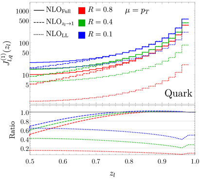
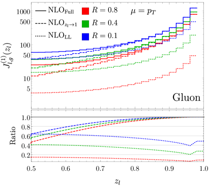
In figure 1 we show how the quark and gluon leading-jet functions depend on in the left and right panels respectively. To clarify the discussion, we set so that the jet function involves only terms and not logarithms involving any other scales. We display each jet function integrated over bins of width . The last bin in each plot includes an integration over plus distributions and delta functions and gives a large negative contribution which therefore cannot be seen on the log plot. Each plot shows the contribution (dashed lines) compared to the full NLO result (solid lines) for . Below each plot we also show their ratio (plotted as a smooth curve between the bins to highlight the trend), indicating that for both the quark and gluon jet functions, the term accounts for, at best of the full NLO contribution333Note that eq. (8) states that the integral should be zero. This is not apparent in the plot due to the presence of delta function and plus distributions which give large negative contributions at ., and only for very small values and at moderate values of .
We also examine limit of the leading-jet functions, where almost all of the jet momentum is carried by a single parton. This limit is interesting because of the soft singularity of QCD, and the NLO results for the jet functions reduce to
| (16) |
where , , and
| (17) |
These contributions are also shown in figure 1 (dotted lines). Here we see that indeed, for , these contributions account for of the value of the jet functions. Of course, this is only a comparison of the corrections, and furthermore these functions appear in cross sections through convolutions with appropriate hard functions. We will investigate the validity of these approximations of the jet functions at the cross section level in section 4.
3 Leading-logarithmic renormalization group equation and solution
In section 3.1, we derive the RGEs for the (sub)leading-jet functions, using a parton shower picture that is accurate to LL order. Our analytical solution to this RGE at order is presented in section 3.2, and we also discuss how this can be extended numerically to all-orders in .
3.1 Deriving the renormalization group equation
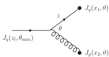
At LL accuracy, we can think of the radiation produced by a parton as a tree of subsequent splittings that are strongly ordered in angle, i.e. the angle of subsequent splittings are parametrically smaller. The RGE can now be derived by considering a single splitting, pictured in figure 2, and noting that the momentum fraction of the leading jet can be calculated recursively (see also ref. Elder:2017bkd ). Specifically, the leading-jet function for the initial parton can be obtained from the leading-jet functions of the two daughter partons, by accounting for the distribution in the momentum fractions and and angle of the daughters. Denoting the momentum fraction of the leading jet produced by the daughter partons as and , the momentum fraction of the leading jet produced by our initial parton is simply given by
| (18) |
The additional factors of and enter because the momentum fractions are of the leading jet produced by a daughter with respect to the momentum of a daughter.
This allows us to immediately write down a recursive expression for the leading-jet function at LL accuracy. For an initial quark this reads
| (19) | ||||
The expression for an initiating gluon is very similar, with the appropriate replacements for the splitting and jet functions, except that both and splittings contribute. To account for the angular ordering, the jet functions carry the additional argument , which gives the largest angle at which the next splitting can occur. For the initial splitting is assumed to be an order one number. For subsequent splittings the upper limit on the integral is set by the angular ordering condition, while the lower limit is always set by the jet radius parameter . To derive the RGE, it is useful to make a change of variables from to the transverse momentum of the daughter parton with respect to the initial parton
| (20) |
Note that this transverse momentum is the scale at which in eq. (19) is evaluated (treating as order one numbers). Taking the derivative with respect to , we obtain the RGE. From the lower limit of the integral in eq. (20) we also read off the natural scale of the jet functions to be .
For a parton of type , we find for the leading-jet function
| (21) |
where
| (22) |
Here and in the following we suppress the dependence on the scale in the arguments of each of the jet functions, to keep the notation compact.
We can similarly derive the LL accurate RGE for the subleading-jet function. We find
| (23) | ||||
where
| (24) |
Note that the constrains and for are automatically satisfied by the jet functions and follow from their definition.
3.2 Solving the renormalization group equation
We now use eq. (21) to generate higher order terms in for the LL solution of the leading-jet functions from lower order ones. It is straightforward to check that inserting the LO solutions into eq. (21) yields the LL part of in eq. (15),
| (25) |
Inserting into eq. (21) and expanding everything to order we obtain the LL terms at order . For the quark leading-jet function these are
| (26) |
where
| (27) |
The analogous result for the gluon jet function can be found in appendix A. At this order there can be as many as three jets in the final state, so the emergence of the new region is expected.
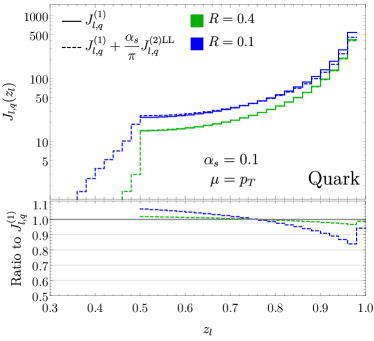
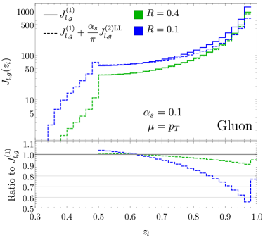
In figure 3 we show the effect of the NNLO corrections as calculated in eqs. (3.2) and (A) on the NLO quark (left) and gluon (right) leading-jet functions as a function of with . The solid curves in each plot show the full NLO jet functions, while the dashed curves show the effect of adding the NNLO LL terms, weighted appropriately by for comparison and where we have set . We show results for (green) and (blue) and the lower panel in each plot displays the ratio compared to the pure NLO prediction for . The LL contributions at NNLO have an integrable divergence as approaches from below. This arises from a soft divergence: the momentum fraction of the softest of the three jets is bound from below by , leading to a in the and color structures in eq. (27). It is clear from the ratio plots, that the NNLO LL corrections for have a smaller impact on the quark jet function, where they are below , than for the gluon where they approach for larger . It is only for more extreme values of that the corrections become significant, again particularly for the gluon leading-jet function at large . However, given that the LL terms at NLO are not a good approximation for the full NLO jet functions, we might expect the same to occur at NNLO.
Moving on to the subleading-jet function, we find that the contribution to the LL evolution is given by
| (28) |
where
| (29) |
and
| (30) |
Eq. (3.2) can be interpreted as a perturbative splitting into partons with momentum fractions and , where the parton with subsequently splits into two partons with momentum fractions and . The splitting probabilities are encoded in eq. (3.2), and the three terms on the last line of eq. (3.2) correspond to the different assignments of leading and subleading jets over these three partons. We have checked that the integral of eq. (3.2) over reproduces in eqs. (3.2) and (A).
Up to this point we have only discussed perturbative solutions to the RG equations in eqs. (21) and (23), obtaining analytic results up to order . The non-linear nature of these equations makes them difficult to solve, and, as has already been suggested, the inclusion of the LL terms alone will not yield a reliable approximation (which will be demonstrated at the level of the cross section in section 4). Nonetheless, it is instructive to investigate all-orders solutions to the RGEs derived here. To this end we introduce the cumulant of the leading-jet functions as
| (31) |
from which the original distribution can be easily obtained using
| (32) |
The advantage of working with cumulants is the regularization of the distribution-valued contributions to the jet function. We can rewrite eq. (21) in terms of cumulants, yielding
| (33) |
In obtaining this expression, we have made use of the sum rule eq. (8). It is possible to solve eq. (3.2) using a Runge-Kutta algorithm or similar. We note that for , the above RGEs linearize and become simple convolutions, which can be solved to all orders by making use of a Mellin transform.
4 Application to Higgs + 1 jet production at the LHC
In this section we present some applications of the (sub)leading-jet function to Higgs + 1 jet production. In section 4.1 we describe how we obtain the singular NLO cross section (in particular the one-loop hard function) for the jet and Higgs transverse momentum spectrum. In section 4.2 we assess the size of the power corrections to the factorization formula in eq. (3) at NLO, and the effect of the terms at order and beyond.
4.1 Construction of NLO predictions
As discussed in section 1, the subleading-jet function can be used to describe exclusive jet production with a loose veto on the momenta of additional jets. The relevant factorization is given in eq. (3), which we write here as
| (34) |
We denote the factorized (singular) expression for the cross section by and on the last line introduce a shorthand notation that will be convenient for our discussion below. Expanding the right-hand side of eq. (4.1) to NLO, we obtain
| (35) |
As noted below eq. (1), is simply the LO partonic cross section for the production of a Higgs boson and a parton . Since the LO subleading-jet functions are simply delta functions, convolutions involving them are trivial and the first term on the right-hand side is just the LO cross section for H+jet production . While can be computed directly from the hard scattering, here we instead extract it from the known full NLO cross section. It can be extracted from eq. (4.1) by replacing with at small values of (we took ) to minimize the corrections. Since is independent of , it can be used for other values of once it has been extracted. Explicitly
| (36) |
In eq. (4.1) the left hand side is essentially since the leading order jet functions with which it is convolved are delta functions.
We can also use the (sub)leading-jet functions to investigate the transverse momentum spectra of the colorless object (in our case the Higgs boson) recoiling against the jets. To derive the corresponding expression, we first make all cross sections in eq. (4.1) also differential in the Higgs transverse momentum and then integrate over . Specifically,
| (37) |
At LO, , so the first term on the right-hand side is the same as for the singular cross section with the measurement. In the last term of eq. (4.1), allowing us to rewrite this term as
| (38) |
The final ingredient required for the Higgs spectrum is the second term on the right-hand side of eq. (4.1). Since this term is independent of , it can again be extracted from the full NLO result at small jet radius .
4.2 Comparison with full NLO predictions
We will now perform a phenomenological study using the cross sections derived in section 4.1. In our numerical results, we take the Higgs mass GeV and vacuum expectation value GeV. We set the factorization and renormalization scales equal to the transverse mass of the Higgs boson, , and restrict the jets to the pseudo-rapidity range . Predictions for NLO distributions are obtained from MCFM-8.3 Campbell:1999ah ; Campbell:2011bn ; Campbell:2015qma , which makes use of virtual matrix elements calculated in refs. Schmidt:1997wr ; Ravindran:2002dc , with the anti- jet clustering algorithm Cacciari:2008gp . We employ the NNLO PDF4LHC15 parton distributions Butterworth:2015oua , within the LHAPDF-6.2.3 framework Buckley:2014ana . We have chosen to use NNLO PDFs to match the order of our results at the end of this section which include corrections. This avoids effects from using PDFs at different orders, which would otherwise obscure the size of the corrections coming from the terms, which we are ultimately interested in.
As a first step, it is insightful to check how good of an approximation the factorized differential cross sections in eqs. (4.1) and (4.1) are to the full NLO predictions.
To this end we show in figure 4 the differential cross section for the jet (left) and Higgs (right) transverse momentum distribution in exclusive Higgs + 1 jet production. In the upper panels the full NLO predictions for and (solid red and blue lines) and the singular cross section (dashed lines) are shown. For comparison the leading order cross section (solid black line) is shown. Taking GeV ensures that there is not too large a hierarchy between and other hard scales, i.e. , since the calculation would otherwise require additional resummation. While , the Higgs distribution extends down to GeV. However, the veto at GeV gives rise to a “Sudakov shoulder” Catani:1997xc in the spectrum around and so we therefore use one large bin accounting for all of the cross section at GeV.444Any detailed predictions in this low-energy part of the spectrum would anyway be outside the range of validity of our factorization. A double differential resummation in this region is performed in Monni:2019yyr . It is clear from the figure that the expansion in small works well, as evidenced by the ratio plots in the lower panels of the figure. In the lower panels the lighter lines show the ratio , with fluctuations due to the limited statistics of the Monte Carlo integration, while the thicker lines display a linear fit in order to highlight the trend. For the Higgs distribution we perform this fit only for GeV to avoid the influence of the Sudakov shoulder. While both values of the jet radius considered are in excellent agreement with the full NLO prediction, delivering predictions typically within a few percent of the exact NLO, factorized predictions for smaller radii give a more accurate prediction of the full NLO, as expected. The validity of the small approximation for relatively large values of has been noted before in e.g. refs. Mukherjee:2012uz ; Dasgupta:2016bnd .
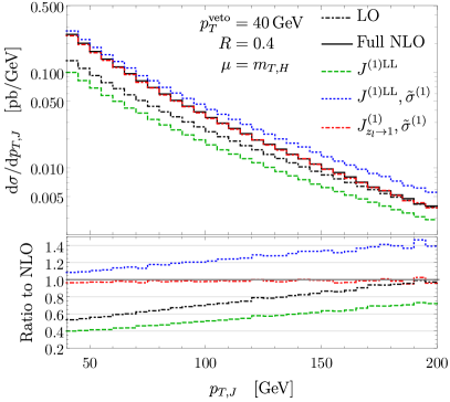
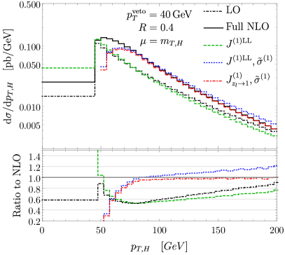
Given that the collinear approximation works so well, we next investigate how much of this is is captured by the terms in the singular cross section. In figure 5 we show the (left) and (right) distributions for , keeping various components of the singular cross section. Shown are predictions obtained by simply adding the LL terms at to the LO cross section (green dashed) as well as the NLO singular cross section, eq. (4.1), using the LL (blue dotted) and soft (red dot-dashed) approximation of the full NLO jet function. The LO (dot-dashed black line) and full NLO (solid black line) contribution are shown for comparison. The bottom panel of each plot displays the ratio of each prediction to the full NLO result. For both the and distributions, we see that simply augmenting the LO cross section with the terms (green dashed line) gives results which severely underestimate the exact NLO cross section. Indeed, from the ratio plots we can see that it only captures between – of the cross section for the distribution depending on the bin and does only slightly better (away from the Sudakov shoulder) for . The use of the LL approximation of the NLO jet function in singular cross section prediction (blue dashed lines) leads to a much better approximation of the full NLO prediction, though the results are typically overestimated and only get worse for larger transverse momentum. This is line with what we observed in figure 1, where the term accounts for only – of the full NLO jet function at across the full range of . In figure 1 we also noted that the soft limit of the jet function in eq. (16) gives a much more faithful approximation of the full result. Using this soft approximation of the jet function in the NLO singular cross sections eqs. (4.1) and (4.1) (red dot-dashed lines) yields results which are almost identical to the complete NLO results for and, outside the influence of the Sudakov shoulder, for .
The overriding conclusion of these studies is that while the limit works extremely well, even for “large” values (e.g. ), the dominant effects here are not given by the corrections to the LO result. This is perhaps unsurprising given that the NLO (and higher) QCD corrections to Higgs + jet production are sizable, so that we might expect large corrections from the NLO hard function . However, it is also clear that the jet function gives an important contribution, of which the term provides a poor approximation. Interestingly though, since the contribution from the terms is negative (the cross section is smaller than the LO result), using smaller values of only makes this a worse approximation to the full NLO result.
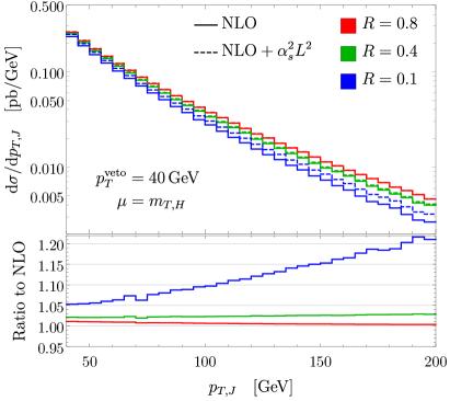
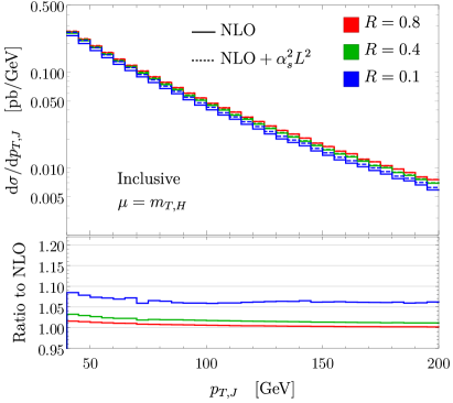
Finally, even though we have established that simply augmenting the LO results with corrections does not provide a good approximation of the full NLO, we can still assess how big an impact the terms have. In figure 6 we show a comparison between the exact NLO prediction (solid lines) and the NLO prediction plus the leading terms (dashed lines) for the jet transverse momentum spectrum at varying values of . In the left plot, we show the exclusive cross section with a loose jet veto GeV where we see that for moderate values of the effect of the terms is minimal. As can be seen in the lower panel, the effect is around – for and at most for . It is only for the more extreme value of that the terms start to have a large impact, especially at large transverse momentum. The more pronounced dependence at has a simple explanation: the transverse momentum dependence of the term is similar to that of the LO cross section, which falls off slower than the exclusive NLO cross section, an effect which is enhanced for smaller values (c.f. and predictions in figure 4). As such, the contribution from the terms, as a fraction of the NLO predictions, grows at larger for these smaller values of . While this is potentially an interesting indication of where terms could become large enough to warrant resummation, it is also well known that the NNLO QCD corrections to Higgs plus jet production cross sections lead to large -factors Chen:2014gva ; Boughezal:2015aha . We would therefore also expect large corrections from the term in the factorization formula, as well as potentially large contributions from . The plot on the right of figure 6 instead displays the inclusive cross section, where we also assess the impact of the terms. In this instance the effect of the terms is relatively unchanged for , while the enhancement seen for in figure 6 is reduced to enhancement for most of the spectrum. Thus, the simple inclusion of these terms cannot lead to the kind of K-factors needed to approximate the full NNLO inclusive cross section.
5 Conclusion
In this paper we have explored the validity of the small approximation and the impact of terms, developing the general framework and showing results for Higgs plus jet production. To describe the transverse momentum spectrum of the hardest jet in the final state (possibly with a loose veto on additional jets), we introduced (sub)leading-jet functions that describe the momentum fractions of the (second) hardest jet produced by a hard parton. We have calculated these jet functions for quarks and gluons to next-to-leading order in QCD. This calculation revealed that these jet functions are poorly approximated when only the terms are retained, even for , but are well described by their soft limit. Using a recursive parton shower picture, we derived the renormalization group equations for the jet functions at leading logarithmic accuracy. These RGEs have an interesting non-linear structure, and so their all-orders solution lends itself to more numerical methods. Nonetheless we used it to produce analytical results for the LL terms at NNLO.
We assessed the impact of these jet functions at the cross section level in the concrete example of exclusive Higgs + 1 jet production with a loose transverse momentum veto on additional jets. We confirmed the validity of the collinear factorization as an approximation to the full cross section at NLO, even for the large value of . Furthermore, we showed that the NLO cross section is not well approximated by simply augmenting the LO result with the terms at NLO. The NLO corrections to the hard scattering are substantial, as is well-known for Higgs production, but also the other contributions to the jet function cannot be neglected. Finally, using our analytic results for the contribution to the NNLO jet functions, we investigate their effect on the cross section. We find that the impact of these logarithms lies at the few percent level, except for rather small values of in exclusive cross sections.
In conclusion, we have found that for describing the leading jet, the collinear approximation also works rather well, even for rather large values of . On the other hand, the corresponding terms in the cross section are not particularly large, suggesting that their resummation is of limited importance. This can of course change as jet substructure techniques utilize subjets with smaller radii, requiring the role of higher order subjet radius logarithms to be reassessed. This may be particularly interesting for track-based observables, where small angular scales are experimentally accessible.
Acknowledgements.
This work is supported by the ERC grant ERC-STG-2015-677323, and the D-ITP consortium, a program of the Netherlands Organization for Scientific Research (NWO) that is funded by the Dutch Ministry of Education, Culture and Science (OCW).Appendix A Higher order solution for gluon leading-jet function
In this appendix we present the LL solution for the gluon leading-jet function at order
| (39) |
where
| (40) |
References
- (1) ALICE collaboration, Exploration of jet substructure using iterative declustering in pp and Pb-Pb collisions at LHC energies, 1905.02512.
- (2) ATLAS collaboration, Measurement of jet-substructure observables in top quark, boson and light jet production in proton-proton collisions at TeV with the ATLAS detector, JHEP 08 (2019) 033 [1903.02942].
- (3) G. F. Sterman and S. Weinberg, Jets from Quantum Chromodynamics, Phys. Rev. Lett. 39 (1977) 1436.
- (4) F. Aversa, M. Greco, P. Chiappetta and J. P. Guillet, Jet Production in Hadronic Collisions to O (), Z. Phys. C46 (1990) 253.
- (5) E. Gerwick, S. Schumann, B. Gripaios and B. Webber, QCD Jet Rates with the Inclusive Generalized kt Algorithms, JHEP 04 (2013) 089 [1212.5235].
- (6) T. Becher, M. Neubert, L. Rothen and D. Y. Shao, Effective Field Theory for Jet Processes, Phys. Rev. Lett. 116 (2016) 192001 [1508.06645].
- (7) T. Becher, M. Neubert, L. Rothen and D. Y. Shao, Factorization and Resummation for Jet Processes, JHEP 11 (2016) 019 [1605.02737].
- (8) Y.-T. Chien, A. Hornig and C. Lee, Soft-collinear mode for jet cross sections in soft collinear effective theory, Phys. Rev. D93 (2016) 014033 [1509.04287].
- (9) S. Alioli and J. R. Walsh, Jet Veto Clustering Logarithms Beyond Leading Order, JHEP 03 (2014) 119 [1311.5234].
- (10) M. Dasgupta, F. Dreyer, G. P. Salam and G. Soyez, Small-radius jets to all orders in QCD, JHEP 04 (2015) 039 [1411.5182].
- (11) A. Banfi, F. Caola, F. A. Dreyer, P. F. Monni, G. P. Salam, G. Zanderighi et al., Jet-vetoed Higgs cross section in gluon fusion at N3LO+NNLL with small- resummation, JHEP 04 (2016) 049 [1511.02886].
- (12) D. W. Kolodrubetz, P. Pietrulewicz, I. W. Stewart, F. J. Tackmann and W. J. Waalewijn, Factorization for Jet Radius Logarithms in Jet Mass Spectra at the LHC, JHEP 12 (2016) 054 [1605.08038].
- (13) M. Dasgupta, F. A. Dreyer, G. P. Salam and G. Soyez, Inclusive jet spectrum for small-radius jets, JHEP 06 (2016) 057 [1602.01110].
- (14) Z.-B. Kang, F. Ringer and I. Vitev, The semi-inclusive jet function in SCET and small radius resummation for inclusive jet production, JHEP 10 (2016) 125 [1606.06732].
- (15) L. Dai, C. Kim and A. K. Leibovich, Fragmentation of a Jet with Small Radius, Phys. Rev. D94 (2016) 114023 [1606.07411].
- (16) C. W. Bauer, S. Fleming and M. E. Luke, Summing Sudakov logarithms in B —¿ X(s gamma) in effective field theory, Phys. Rev. D63 (2000) 014006 [hep-ph/0005275].
- (17) C. W. Bauer, S. Fleming, D. Pirjol and I. W. Stewart, An Effective field theory for collinear and soft gluons: Heavy to light decays, Phys. Rev. D63 (2001) 114020 [hep-ph/0011336].
- (18) C. W. Bauer and I. W. Stewart, Invariant operators in collinear effective theory, Phys. Lett. B516 (2001) 134 [hep-ph/0107001].
- (19) C. W. Bauer, D. Pirjol and I. W. Stewart, Soft collinear factorization in effective field theory, Phys. Rev. D65 (2002) 054022 [hep-ph/0109045].
- (20) M. Beneke, A. P. Chapovsky, M. Diehl and T. Feldmann, Soft collinear effective theory and heavy to light currents beyond leading power, Nucl. Phys. B643 (2002) 431 [hep-ph/0206152].
- (21) X. Liu and F. Petriello, Resummation of jet-veto logarithms in hadronic processes containing jets, Phys. Rev. D87 (2013) 014018 [1210.1906].
- (22) X. Liu and F. Petriello, Reducing theoretical uncertainties for exclusive Higgs-boson plus one-jet production at the LHC, Phys. Rev. D87 (2013) 094027 [1303.4405].
- (23) P. F. Monni, L. Rottoli and P. Torrielli, Higgs transverse momentum with a jet veto: a double-differential resummation, 1909.04704.
- (24) H.-M. Chang, M. Procura, J. Thaler and W. J. Waalewijn, Calculating Track-Based Observables for the LHC, Phys. Rev. Lett. 111 (2013) 102002 [1303.6637].
- (25) B. T. Elder, M. Procura, J. Thaler, W. J. Waalewijn and K. Zhou, Generalized Fragmentation Functions for Fractal Jet Observables, JHEP 06 (2017) 085 [1704.05456].
- (26) W. T. Giele and E. W. N. Glover, Higher order corrections to jet cross-sections in e+ e- annihilation, Phys. Rev. D46 (1992) 1980.
- (27) V. N. Gribov and L. N. Lipatov, Deep inelastic e p scattering in perturbation theory, Sov. J. Nucl. Phys. 15 (1972) 438.
- (28) G. Altarelli and G. Parisi, Asymptotic Freedom in Parton Language, Nucl. Phys. B126 (1977) 298.
- (29) Y. L. Dokshitzer, Calculation of the Structure Functions for Deep Inelastic Scattering and e+ e- Annihilation by Perturbation Theory in Quantum Chromodynamics., Sov. Phys. JETP 46 (1977) 641.
- (30) W. J. Waalewijn, Calculating the Charge of a Jet, Phys. Rev. D86 (2012) 094030 [1209.3019].
- (31) J. M. Campbell and R. K. Ellis, An Update on vector boson pair production at hadron colliders, Phys. Rev. D60 (1999) 113006 [hep-ph/9905386].
- (32) J. M. Campbell, R. K. Ellis and C. Williams, Vector boson pair production at the LHC, JHEP 07 (2011) 018 [1105.0020].
- (33) J. M. Campbell, R. K. Ellis and W. T. Giele, A Multi-Threaded Version of MCFM, Eur. Phys. J. C75 (2015) 246 [1503.06182].
- (34) C. R. Schmidt, H —¿ g g g (g q anti-q) at two loops in the large M(t) limit, Phys. Lett. B413 (1997) 391 [hep-ph/9707448].
- (35) V. Ravindran, J. Smith and W. L. Van Neerven, Next-to-leading order QCD corrections to differential distributions of Higgs boson production in hadron hadron collisions, Nucl. Phys. B634 (2002) 247 [hep-ph/0201114].
- (36) M. Cacciari, G. P. Salam and G. Soyez, The anti- jet clustering algorithm, JHEP 04 (2008) 063 [0802.1189].
- (37) J. Butterworth et al., PDF4LHC recommendations for LHC Run II, J. Phys. G43 (2016) 023001 [1510.03865].
- (38) A. Buckley, J. Ferrando, S. Lloyd, K. Nordström, B. Page, M. Rüfenacht et al., LHAPDF6: parton density access in the LHC precision era, Eur. Phys. J. C75 (2015) 132 [1412.7420].
- (39) S. Catani and B. R. Webber, Infrared safe but infinite: Soft gluon divergences inside the physical region, JHEP 10 (1997) 005 [hep-ph/9710333].
- (40) A. Mukherjee and W. Vogelsang, Jet production in (un)polarized pp collisions: dependence on jet algorithm, Phys. Rev. D86 (2012) 094009 [1209.1785].
- (41) X. Chen, T. Gehrmann, E. W. N. Glover and M. Jaquier, Precise QCD predictions for the production of Higgs + jet final states, Phys. Lett. B740 (2015) 147 [1408.5325].
- (42) R. Boughezal, C. Focke, W. Giele, X. Liu and F. Petriello, Higgs boson production in association with a jet at NNLO using jettiness subtraction, Phys. Lett. B748 (2015) 5 [1505.03893].