Fundamental Parameters of 30,000 M dwarfs in LAMOST DR1
Using Data-driven Spectral Modeling
Abstract
M dwarfs are the most common type of star in the Galaxy, and because of their small size are favored targets for searches of Earth-sized transiting exoplanets. Current and upcoming all-sky spectroscopic surveys, such as the Large Sky Area Multi-Object Fiber Spectroscopic Telescope (LAMOST), offer an opportunity to systematically determine physical properties of many more M dwarfs than has been previously possible. Here we present new effective temperatures, radii, masses, and luminosities for 29,678 M dwarfs with spectral types M0—M6 in the first data release (DR1) of LAMOST. We derived these parameters from the supervised machine learning code, The Cannon, trained with 1,388 M dwarfs in the Transiting Exoplanet Survey Satellite (TESS) Cool Dwarf Catalog that were also present in LAMOST with high signal-to-noise ratio (250) spectra. Our validation tests show that the output parameter uncertainties are strongly correlated with the signal-to-noise of the LAMOST spectra, and we achieve typical uncertainties of 110 K in (3%), 0.065 (14%) in radius, 0.054 (12%) in mass, and 0.012 (20%) in luminosity. The model presented here can be rapidly applied to future LAMOST data releases, significantly extending the samples of well characterized M dwarfs across the sky using new and exclusively data-based modeling methods.
tablenum \restoresymbolSIXtablenum
1 Introduction
M dwarfs are preferred targets for exoplanet hunting due to their status as the most common stellar type in the galaxy. (e.g., Mann et al. 2015), and for their potential in detecting Earth and super-Earth sized exoplanets using both ground and space-based telescopes via radial velocity measurements and transit detection (e.g. Shields et al. 2016). The fundamental properties of any host star such as radius and mass need to be known to a reasonable degree of certainty in order to characterize the exoplanets they host.
For nearby, bright, well-known M dwarf samples identified via, e.g., very high proper motions (e.g., Lépine et al. 2013), precise stellar properties can be estimated from broadband colors and parallax alone. For example, Mann et al. (e.g., 2019, 2015) have developed empirical calibrations that permit the determination of radii and masses of M-dwarfs to better than 10% precision from near-infrared colors and a near-infrared absolute magnitude. However, for the multitude of M dwarfs that have not yet been identified or characterized by such catalogs, there remains a need to develop robust spectroscopic methods which can circumvent problems associated with reddening that can negatively affect color-based methods, and additionally leverage current and upcoming large-scale spectroscopic surveys.
However, automated M dwarf characterization via stellar spectroscopy with synthetic models is difficult given the complicated nature of their stellar atmospheres. For example, generating model synthetic spectra for stars cooler than FGK-types, such as M dwarfs, is difficult because of the formation of molecules in their photospheres e.g., TiO, VO, and CaH in the optical, and H2O and CO in the near-IR ( e.g., Rojas-Ayala et al. 2012; Shields et al. 2016). Very heavy absorption can be observed in an M dwarf spectrum by the presence of molecular compounds which are allowed under their lower effective temperatures ( 3850 K), which lead to broad and overlapping spectral lines that can be hard to parse ( e.g., Rojas-Ayala et al. 2012). Modeling the absorption lines of these compounds is incomplete (e.g., Allard et al. 2011; Husser et al. 2013), and the lack of a well-defined continuum is also expected, with some wavelength regions being completely saturated with absorption features, making normalization for standard spectroscopic analysis also difficult. Additional complications due to the stars’ intrinsic properties are deep convection cells and magnetic activity/rapid rotation, effects that in general are not included in models of low-mass stellar atmospheres.
The low luminosities of these stars also brings restrictions to both of these methods; parallax of dwarfs can only be obtained for the very brightest, and quality (high signal-to-noise ratio) spectra are difficult to obtain. A common method of practice is to also parameterize the properties of dwarfs if they are in binary with FGK-type companions, but these are limited to a select number of dwarfs.
The result is that physics-based models are incomplete and computationally expensive for M dwarfs which make the method of fitting to synthetic spectra difficult. This presents a problem—there is a high demand for M dwarf basic properties for exoplanet and stellar population characterization, but there is much room for improvement in automated analysis in terms of both computational speed and accuracy.
A promising alternative is using data-based modeling approaches that use machine learning to predict what a spectrum would look like given its stellar properties, and then infer those properties of uncharacterized spectra based on the model. We discuss in this work how The Cannon 111https://github.com/annayqho/TheCannon (Ness et al. 2015) can successfully model low resolution, low to moderate signal-to-noise M dwarf spectra, and we use The Cannon model to find the properties of 29,678 previously uncharacterized optical spectra of M dwarfs in the LAMOST DR1 catalog.
The Cannon has so far been successfully applied to characterize red giants using APOGEE spectra and LAMOST spectra and using parameters derived via the ASPCAP pipeline (Ho et al. 2017a, b). The Cannon has also been applied to much higher resolution than LAMOST M dwarf spectra (Behmard et al. 2019). LAMOST is an optical spectroscopic survey all-sky survey for the Northern celestial hemisphere (Luo et al. 2015). There are 121,000 M dwarf spectra in the first data release (DR1), the majority of which have not yet been characterized beyond a simple spectral subtype determined from color photometry. We cross-match the LAMOST targets with the TESS Cool Dwarf Catalog (Muirhead et al. 2018), from which we create a training set to train a spectral model using The Cannon.
In Section 2, we summarize the data selection and preparation in this work. In Section 3, we discuss the methods by which we chose an optimal training set for accuracy and the testing set for applicability. We also discuss the methods by which we assessed the model’s accuracy in determining basic parameters: , radius, mass, and luminosity. In Section 4, we report these properties and their uncertainties for the 29,678 M dwarfs in LAMOST DR1 for which we were able to determine reliable properties. Finally, Section 5 concludes with a summary of our conclusions.
2 Data
In this section, we describe the data that we use, their preparation for use with The Cannon, and quality control steps taken to train, validate, and apply The Cannon model to reliable data.
The data are drawn from two main catalogs: (1) the LAMOST first data release (DR1) M dwarf catalog, is the spectral data set that we wish to classify (Luo et al. 2015), and (2) the TESS Cool Dwarf Catalog (TCD) (Muirhead et al. 2018), whose parameters we utilize for training and validation of The Cannon model. The parameters from the TCD (Muirhead et al. 2018) on which we have chosen to train The Cannon model are effective temperature (), radius (), mass (), and luminosity (); these are the parameters that we will therefore be able to estimate for the LAMOST DR1 stars.
Our data are split into three subsets, following the approach described by Ness et al. (2015). The subset of 30,152 TCD stars for which we also have LAMOST spectra (hereafter, the cross-matched TCD) are divided into a training set and a validation set. The training set contains the highest signal-to-noise ratio (SNR) spectra of all TCD and LAMOST cross-matches, paired with their known associated stellar characteristics or parameters (i.e., labels in Ness et al. 2015); the training set is used to generate the data-driven model. The validation set is the remaining cross-matched TCD stars that were not used in the training set but whose parameters are known and therefore can be used to assess the fidelity of the model. The LAMOST stars that are included in neither the training set nor the validation set comprise the survey set. These are spectra we wish to characterize using the model we created from the training set, and vetted with the validation set.
2.1 LAMOST DR1 Spectra
The Large Sky Area Multi-Object Fiber Spectroscopic Telescope (LAMOST) is a low resolving power (R 1800), optical/near-infrared (3690–9100Å), ground-based survey (Luo et al. 2015). One of the data products from LAMOST is the LAMOST DR1 M dwarf catalog (Guo et al. 2015), a catalog of stars whose spectra have been classified broadly as being of M spectral type but without more detailed physical information. This catalog consists of 122,677 spectra with simple spectral type classifications from M0 to M9; these spectra represent 103,467 unique objects after excluding any duplicate observations of the same target.
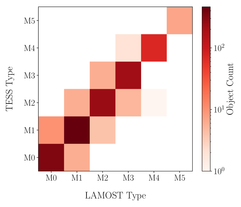
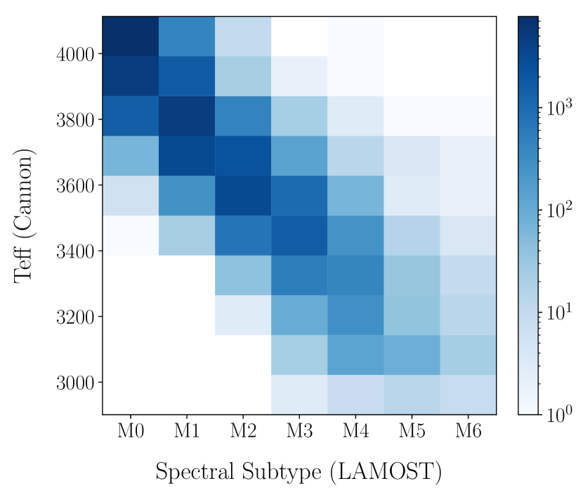
While the LAMOST catalog includes some stars with approximate classifications as late as M9, we chose to include only stars with a LAMOST DR1 spectral subtype of M6 and earlier, given that the training set includes only stars with LAMOST subtypes from M0 to M6 (see Section 3.1). Figure 1 shows the comparison of the LAMOST spectral subtypes to those from the TCD for the 30,152 spectra that were cross-matched, where the relatively small number of objects with the latest spectral types is due to difficulty of observing very faint objects with high signal.
The LAMOST DR1 catalog provides the spectra for each of these stars. We require that to be usable a LAMOST spectrum must include a wavelength solution (), flux (), and flux error (or flux inverse variance; ), the last of which is used as a statistical weight for training a model pixel-by-pixel.
2.1.1 Basic processing of LAMOST spectra
First, we applied a bad pixel mask using the code supplied with The Cannon package for this purpose. The bad pixel mask flagged pixels in the spectra from information provided in the LAMOST meta-data, including poor sky-subtraction, bad CCD pixels, and infinite or negative flux inverse variance values. The mask also manually flagged pixels with strong telluric lines and discontinuities from the joining of LAMOST’s blue and red spectrographs at 5800–6000 Å. For pixels flagged in the bad pixel mask we manually set the inverse variances to a very small value222We chose a value of , as opposed to 0, which helps avoid errors arising from division by zero in future operations..
In order for a spectrum to be input into The Cannon for analysis, the spectra in the training, validation, and survey subsets also must be interpolated to a common wavelength scale with uniform wavelength spacing. From inspection of the spectra we found that the LAMOST data were most consistently free of bad pixels or other problems at wavelengths shorter than 4500Å, and thus we interpolated to a common wavelength range of 4500–7500Å, and used a uniform spacing of 1 Å, as these parameters approximately represent the native format of the LAMOST spectra for M stars. Each resulting spectrum is a data array, with each of the 3000 pixels containing a standardized wavelength, flux, and a flux inverse variance float value.
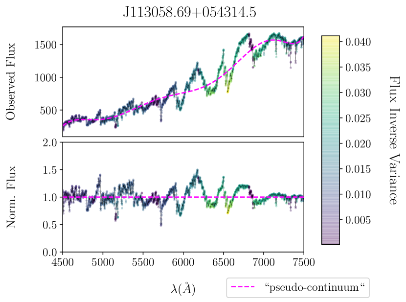
In order to compare fluxes from spectrum to spectrum to create The Cannon model, each spectrum’s continuum must also be normalized. Traditional methods of finding and then dividing an M dwarf’s spectrum by its continuum (continuum-normalization) are challenging because of the complex nature of the stellar spectra as mentioned in Section 1. Therefore, we adopted the so-called “pseudo continuum-normalization” method used by Ho et al. (2017b); Behmard et al. (2019), which first approximates the continuum at wavelength via Gaussian smoothing over pixels and then normalizes the original spectrum with this smoothed fit:
| (1) |
where index represents the sum over pixels, and the individual pixel weights, , are given by:
| (2) |
where , , , is the wavelength, flux, and flux error at the th pixel, respectively. We pseudo-normalized all spectra with a Gaussian width of = 50 Å pixels, which is wider than most broader absorption features, and used the flux inverse variance as weights as recommended by Ho et al. (2017b). The procedure is visualized with an example in Figure 2.
We note that this is not a standard robust normalization, in which the maximum flux is well defined and set to unity, but it is a technique where the spectra can be quantitatively and consistently compared because they are placed on a common flux scale. This pseudo-normalization method sometimes over-fits too deeply into absorption bands (e.g., Figure 2), but because the LAMOST spectra have the same Gaussian function outlined in Ho et al. (2017b) systematically applied, it is the preferable technique as it avoids human or physics-model bias from other standard normalization methods.
Next, LAMOST DR1 objects with no redshift parameter reported in the meta-data cannot be shifted to a rest wavelength frame, a requirement for any spectrum to be input into The Cannon. Approximately 10,000 stars were eliminated for this reason.
Finally, through visual inspection of a random set of the LAMOST spectra for quality checks, some were found to have unusually high flux at blue wavelengths (4500Å and bluer) which is atypical of M dwarf stars and almost certainly not intrinsic. We chose to eliminate 1000 stars based on having especially severe upward trends to the blue, which we defined on the basis of the slope of the pseudo-continuum being more negative than (in units of normalized flux per unit wavelength). The cause of this high blueward flux effect is unclear, but might be due to instrumental, calibration, or sky subtraction error.
2.1.2 Spectrum filtering quality control
We require an objective measure of the quality of the LAMOST spectra, both to select the highest quality subset for training, and to ensure that we do not attempt to classify very poor spectra.
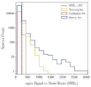
We chose as our quality metric a measure of signal-to-noise ratio (SNR), which we calculated from the sum of the measured SNRs in the individual LAMOST quasi-photometric bands (), hereafter SNRλ. This approach was preferred over the more formal method of using flux error as it is computationally faster and independent of the bad pixel masks, and it is readily obtainable from the LAMOST meta-data. We determined a requirement of SNRλ 50 based on validation testing of the model described in Section 4.3; consequently 45,000 objects with SNRλ 50 were eliminated from any further analysis.
For the training subset, we chose to use a more stringent quality threshold of SNRλ 250 (see Figure 3). These choices of SNRλ thresholds are described more fully in Section 3.2.
2.2 TESS Cool Dwarf Parameters for Training and Validation
The training and validation of The Cannon model requires a set of stars whose physical parameters (i.e., labels in Ness et al. 2015) are known. We adopt the parameters provided in the TCD as the known labels with which to train and validate our model. Those parameters were in turn determined by Muirhead et al. (2018) on the basis of the empirical relations of Mann et al. (2015).
Note that while the TCD was created in order to enhance planet detection around cool dwarfs by the TESS mission, the TCD was created more generally to develop a systematically vetted, brightness and proper-motion limited sample of cool dwarfs across the sky in a manner that is as unbiased as possible. We cross-matched the LAMOST DR1 M-dwarf catalog with the entirety of the 1 million sources in the TCD catalog, not just the TCD targets that were ultimately selected by the TESS mission for 2-minute cadence observations for planet detection. Of course, our training set will necessarily inherit any features inherent in the TCD sample, the most important of which are as follows (see Muirhead et al. 2018): Unresolved binaries will appear to have masses and radii that are too large for their color; metallicities are not known for the majority of the TCD sample, hence we cannot train on metallicity as a data label and we cannot incorporate any metallicity effects into our trained model; the catalogs from which the TCD drew its proper motions were highly incomplete in the Southern hemisphere; and some stars in the TCD relied on inhomogeneous sources of photometry for colors.
Upon a quality check examination of vs. and vs. for these stars, we found a small number of stars whose TCD parameters deviate from the Mann et al. (2015) empirical relations. These outliers are most likely the result of inhomogeneous sources of photometry for some stars and/or unresolved binaries, as noted above.
In order to ensure consistency in the parameters used for the training, we eliminated these 18 outlier stars that deviated in by more than 0.01 and in by more than 0.01 .
3 Methods
In this section we discuss the methods for ensuring the accuracy of the model produced by The Cannon for M dwarfs and detail how we further optimized the data-driven model by choosing appropriate SNRλ minimum cutoffs for training, validation, and survey sets.
Parameter uncertainties are currently not incorporated in The Cannon’s generative modeling; broadly, the model output uncertainties are formal uncertainties based on the flux error and closeness of the model fit to a spectrum. We therefore determine more robust uncertainties on the output parameters using the scatter of the validation set about known parameters for the 30,152 TCD/LAMOST cross-matches, to find a function that estimates parameter error with SNRλ, as described in Section 4.3.
3.1 Model Training
In the first step, we trained The Cannon with the training set of 1,388 stars for which we have high-quality LAMOST spectra as well as parameters (, , , and ) from the TCD (see Section 2.2), and that satisfied the quality control cuts discussed in Section 2.
As outlined in previous work (e.g., Ness et al. 2015; Ho et al. 2017b; Behmard et al. 2019), we can represent a given spectrum’s flux at wavelength , , as the product of the model coefficients and the spectrum’s labels (i.e., physical parameters), , plus noise:
| (3) |
The noise is the quadrature sum of the measurement error in the observed flux, , and the uncertainty in the model coefficients, :
| (4) |
where is a random Gaussian deviate with zero mean and zero unit variance (Ness et al. 2015). For our implementation with training labels taken from the TCD, we define in terms of the physical parameters , , , and , to second order and including cross-terms:
| (5) | ||||
where the first term allows for a linear offset in the fitted flux values (Behmard et al. 2019).
For a given spectrum, , we can then get the single-pixel log likelihood function (), which gives the most likely flux value at a specific wavelength pixel, given model scatter, observational uncertainty, and set of labels:
| (6) |
where the superscript denotes the transpose of the matrix. The Cannon then uses these pixel likelihood probabilities to derive model coefficients that apply to the full set of Ness et al. (e.g., 2015):
| (7) |
The output of this step is a set of model coefficients for each wavelength pixel for each stellar parameter. The data-driven model can now be applied to any other LAMOST spectrum, where the most probable value for a stellar parameter can be calculated given flux and flux error across all pixels.
3.2 Model Validation
Next, to validate The Cannon model, we applied the trained data-driven model from above to the 30,152 stars comprising the validation subset (see Section 2). We chose 18,844 LAMOST spectra after the same quality checks described in 2, except the SNRλ minimum is reduced to 50. Figure 4 shows the results of the validation, in which we compare the parameters output by The Cannon to the input values as adopted from the TCD.
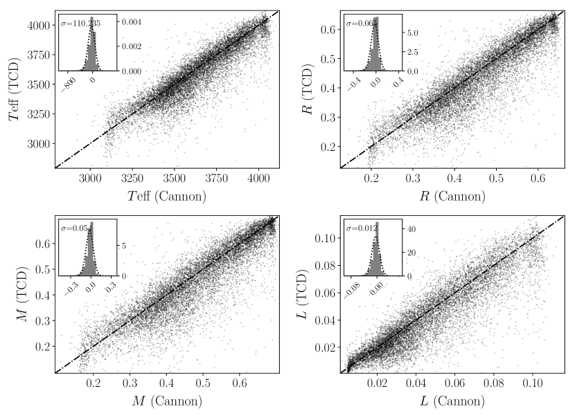
Overall, we observe good one-to-one agreement between the TCD input and The Cannon output labels for the validation set in all four of the training labels (, , , and ). The scatter about the one-to-one line of agreement is approximately Gaussian (see the insets in each panel of Figure 4), with Gaussian widths of 100 K, 0.06 , 0.05 , and 0.01 in , , , and , respectively. For reference, the uncertainties in the training labels themselves as reported in the TCD are 100 K, 0.06 , 0.07 , and 0.008 , respectively in Muirhead et al. (2018).
We do observe some slight asymmetry in the residuals about the one-to-one relation, or a “tail” of residuals where The Cannon output labels are a bit larger than the analogous values of TCD input labels. We also observe some evidence for breakdown of the model for the coolest stars, i.e., 3150 K (likely due to the small number of M5–M6 stars in the training set), as well as for the hottest stars, i.e., 4000 K, where the scatter in the residuals become slightly discontinuous and asymmetric (Figure 4). The disagreement at the hotter end (4000 K) is not surprising, as the TCD’s upper limit is 4000 K (Muirhead et al. 2018).
3.3 SNRλ Quality Cutoffs
Several factors such as wavelength range, quantity of objects in the training set, type of continuum-normalization, label choice, and others, can affect the accuracy of the labels derived by our trained model from The Cannon package. In our tests with The Cannon model applied to the LAMOST spectra, we found that SNR of spectra, both for training and validation, was the most important factor for model accuracy.
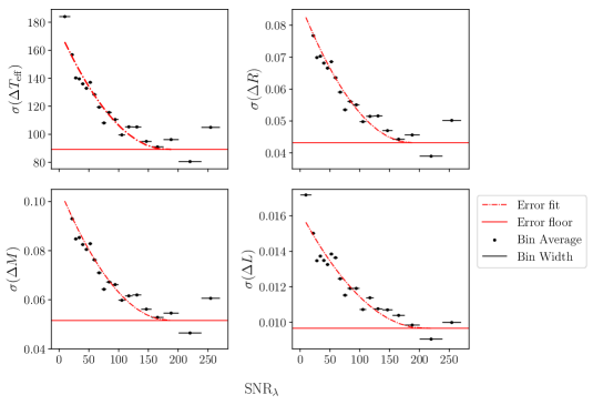
In order to determine an appropriate requirement for SNRλ for both the final training subset described above and for application of the trained model to the final survey set described below, we examined The Cannon’s performance as a function of SNRλ in Figure 5.
We found that the accuracy of the model worsened significantly at SNRλ 50, and so have opted in the final results reported below to exclude such stars. For example, at SNRλ, the scatter in the inferred radii and masses becomes 15% (see Figure 5). In addition, we selected a threshold of SNRλ 250 for the training set, as these represent the very highest quality spectra while still possessing a significant number of objects (2300) to include in the training set. Moreover, inspection of the trends in Figure 5 reveal that the scatter in the inferred parameters does not improve beyond SNRλ, thus we assume that including all objects with SNRλ in the training set will maximize the performance of the trained model. With this cutoff of SNRλ and other quality checks, the final training set consists of 1,388 spectra that are each unique objects (with unique LAMOST designations) out all 24,546 unique objects available that are cross-matches with TCD.
4 Results
After application of the quality and other cuts described in the preceding sections, we have been able to successfully apply The Cannon to 29,678 M dwarfs, for which we report newly characterized , , , and labels. A sample of these final results are reported in Table 1.
| Designation | SNRλ | SpType | |||||||||
|---|---|---|---|---|---|---|---|---|---|---|---|
| J080546.84+202017.8 | 3469.6 | 128.5 | 0.376 | 0.064 | 0.384 | 0.077 | 0.026 | 0.013 | 58.4 | M4 | 1998.0 |
| J064420.73+323838.6 | 3680.1 | 106.8 | 0.481 | 0.054 | 0.513 | 0.063 | 0.049 | 0.014 | 264.2 | M1 | 1899.0 |
| J131151.74+565947.5 | 3837.4 | 99.0 | 0.560 | 0.049 | 0.607 | 0.059 | 0.070 | 0.012 | 119.9 | M1 | 1312.0 |
| J095520.46+301012.0 | 3732.4 | 129.2 | 0.513 | 0.064 | 0.551 | 0.077 | 0.055 | 0.013 | 57.3 | M2 | 3592.7 |
| J100744.45020217.4 | 3995.9 | 124.2 | 0.626 | 0.062 | 0.677 | 0.074 | 0.095 | 0.013 | 65.2 | M0 | 2512.6 |
4.1 Final Eliminations
We note that a small fraction of the stars analyzed and that otherwise satisfied our quality cuts nonetheless failed to be characterized by The Cannon. This was the case for 2,445 stars, for which at least one or more of the output labels failed, identified by NaN or negative label values.
We visually inspected these failed cases, noting that in many instances the LAMOST spectrum had a very large positive or negative outlier feature, perhaps due to bad pixels that were not masked. However, there were also instances where visually the spectrum did not appear unusual. There were no other obvious trends in the characteristics of the failed spectra; they covered a large SNRλ range and included both early and late subtypes. In conclusion, we were not able to determine an obvious common cause for this failure. In any case, these have been completely removed from our final characterized set in Table 1 and what is shown in Figures 6, 7, and 8.
Finally, we also eliminated a small number of stars whose final goodness-of-fit statistic () from The Cannon was very poor. This is shown in Figure 6, where we adopted a cutoff of 5,000, corresponding to a of 3 per degree of freedom.

4.2 Model Parameters
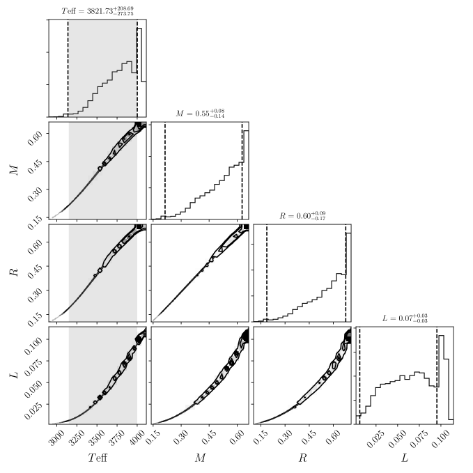
The parameters of the M dwarfs The Cannon has calculated from LAMOST DR1 spectra are as expected for their spectral types. Their ranges are 29014113 K, 0.140.66 , 0.100.71 , and 0.0020.115 . Note that the relatively smaller number of characterized stars at the coolest (latest spectral subtypes) is at least in part due to our quality cuts that require SNRλ and that our training set had fewer stars in this range.
While the LAMOST pipeline does not provide a estimate for most M dwarfs in the catalog, the catalog does provide an estimated subtype, which we used as a sanity check on the output by our trained model (see Figure 7). We find that there is a reasonable progression from higher to lower derived from The Cannon corresponding to increasingly later subtypes reported by LAMOST. The overall distribution of model-derived parameters of the newly characterized 33,095 LAMOST spectra can be seen in Figure 8.
4.3 Error Estimation
As described above, we experimented by running The Cannon with many different training subsets and assessing the impact of different input variables on the scatter in the resulting output parameters. We found that SNRλ is by far the most important predictor of the parameter scatter (see Figure 5) versus other potential factors (e.g., continuum normalization method, different pixel masks, etc). Therefore, we proceed to derive stellar parameter errors for a particular spectrum as a function of its SNRλ. Figure 5 shows the empirical relationship between the standard deviation of the residuals of each label from the validation step and the SNRλ.
We have opted to approximate the relationship between parameter scatter and SNRλ with a simple polynomial function. This is the simplest form that appears to reasonably well represent the empirical relationship—it is not derived from first principles—however, we believe it fully suffices for our purposes here. Table 2 reports the coefficients of the fitted polynomial relationships, which we use to report the final estimated uncertainties on the labels that we report in Table 1.
| units | error floor | ||||
|---|---|---|---|---|---|
| K | |||||
Note. — , where SNRλ.
We do note that the uncertainties we infer in this way for the high SNRλ training sample are very similar to those reported by Muirhead et al. (2018), even though The Cannon model does not incorporate label uncertainties in its training. In other words, the model appears to be naturally reproducing the expected errors for the highest quality sample, effectively setting the error floor for the output parameters.
5 Summary
We were successfully able to extend the range of use for The Cannon in determining properties of M dwarfs to low-resolution, low signal-to-noise, optical spectra. We obtained spectra from the LAMOST DR1 M dwarf catalog and properties from the TESS Cool Dwarf Catalog, and performed a cross-label transfer similar to the procedure detailed in Ho et al. (2017b). First, we performed quality checks on the spectra before implementing the model, such as filtering out poor spectra and establishing minimum signal-to-noise ratio (SNRλ) cutoffs (Section 2.1.2, Section 3.3). We selected a training subset with the best available (SNRλ250) LAMOST spectra that also had reasonable TESS Cool Dwarf Catalog parameters to train the model (Section 2.2). We then assessed the model’s validity and calculated parameter errors as a function of SNRλ (Section 3.2, Section 4.3). We also eliminated objects from our final characterized survey set according to poor and kept only objects for which all four model parameters (, , , ) could be determined successfully.
In the end, were able to apply this method to determine the properties of 30,000 M dwarfs observed by LAMOST that had not been otherwise characterized. We achieve typical uncertainties of 110 K in (3%), 0.065 (14%) in radius, 0.054 (12%) in mass, and 0.012 (20%) in luminosity, driven almost entirely by the precision and range of the training set. The model presented here can be rapidly applied to future LAMOST data releases, significantly extending the samples of well characterized M dwarfs across the sky using new and exclusively data-based modeling methods.
There is room for future improvements. One particular area for improved accuracy would be to incorporate parameter measurement uncertainties as as an additional weight for the model. The Cannon approach can also be sensitive to outliers, especially if the training set is small. We therefore recommend careful scrutiny and removal of outliers, such as by the procedures we adopted in Sections 2.1.2 and 2.2.
Even so, this work demonstrates that The Cannon model can be applied to M dwarfs with a smaller training set than those used in previous works (e.g., Ness et al. 2015, 2016; Ho et al. 2017b, a), and can be used specifically to determine basic stellar properties from LAMOST M dwarf spectra with high accuracy and speed.
References
- Allard et al. (2011) Allard, F., Homeier, D., & Freytag, B. 2011, in Astronomical Society of the Pacific Conference Series, Vol. 448, 16th Cambridge Workshop on Cool Stars, Stellar Systems, and the Sun, ed. C. Johns-Krull, M. K. Browning, & A. A. West, 91
- Behmard et al. (2019) Behmard, A., Petigura, E. A., & Howard, A. W. 2019, arXiv e-prints, arXiv:1904.00094
- Foreman-Mackey (2016) Foreman-Mackey, D. 2016, The Journal of Open Source Software, 24, doi:10.21105/joss.00024
- Guo et al. (2015) Guo, Y.-X., Yi, Z.-P., Luo, A.-L., et al. 2015, Research in Astronomy and Astrophysics, 15, 1182
- Ho et al. (2017a) Ho, A. Y. Q., Rix, H.-W., Ness, M. K., et al. 2017a, ApJ, 841, 40
- Ho et al. (2017b) Ho, A. Y. Q., Ness, M. K., Hogg, D. W., et al. 2017b, ApJ, 836, 5
- Hunter (2007) Hunter, J. D. 2007, Computing in Science & Engineering, 9, 90
- Husser et al. (2013) Husser, T. O., Wende-von Berg, S., Dreizler, S., et al. 2013, A&A, 553, A6
- Lépine et al. (2013) Lépine, S., Hilton, E. J., Mann, A. W., et al. 2013, AJ, 145, 102
- Luo et al. (2015) Luo, A. L., Zhao, Y. H., Zhao, G., et al. 2015, arXiv e-prints, arXiv:1505.01570
- Mann et al. (2015) Mann, A. W., Feiden, G. A., Gaidos, E., Boyajian, T., & von Braun, K. 2015, ApJ, 804, 64
- Mann et al. (2019) Mann, A. W., Dupuy, T., Kraus, A. L., et al. 2019, ApJ, 871, 63
- Muirhead et al. (2018) Muirhead, P. S., Dressing, C. D., Mann, A. W., et al. 2018, AJ, 155, 180
- Ness et al. (2015) Ness, M., Hogg, D. W., Rix, H. W., Ho, A. Y. Q., & Zasowski, G. 2015, ApJ, 808, 16
- Ness et al. (2016) Ness, M., Hogg, D. W., Rix, H. W., et al. 2016, ApJ, 823, 114
- Oliphant (2006) Oliphant, T. E. 2006, A guide to NumPy, Vol. 1 (Trelgol Publishing USA)
- Rojas-Ayala et al. (2012) Rojas-Ayala, B., Covey, K. R., Muirhead, P. S., & Lloyd, J. P. 2012, ApJ, 748, 93
- Shields et al. (2016) Shields, A. L., Ballard, S., & Johnson, J. A. 2016, Phys. Rep., 663, 1