Abstract

The requirement of electroweak naturalness in simple supersymmetric models implies the existence of a cluster of four light higgsinos with mass 100300similar-toabsent100300\sim 100-300 GeV, the lighter the better. While such light compressed spectra may be challenging to observe at LHC, the International Linear e+esuperscript𝑒superscript𝑒e^{+}e^{-} Collider (ILC) with s>2mhiggsino𝑠2subscript𝑚higgsino\sqrt{s}>2m_{\rm higgsino} would serve as both a SUSY discovery machine and a precision microscope. We study higgsino pair production signatures at the ILC based on full, Geant4-based simulation of the ILD detector concept. We examine several benchmark scenarios that may be challenging for discovery at HL-LHC due to mass differences between the higgsino states between 202020 and 444 GeV. Assuming s=500𝑠500\sqrt{s}=500 GeV and 1000 fb-1 of integrated luminosity, the individual higgsino masses can be measured to 12%1percent21-2\% precision in case of the larger mass differences, and at the level of 5%percent55\% for the smallest mass difference case. The higgsino mass splittings are sensitive to the electroweak gaugino masses and allow extraction of gaugino masses to 320%similar-toabsent3percent20\sim 3-20\% (depending on the model). Extrapolation of gaugino masses via renormalization group running can test the hypothesis of gaugino mass unification. We also examine a case with natural generalized mirage mediation where the unification of gaugino masses at an intermediate scale apparently gives rise to a natural SUSY spectrum somewhat beyond the reach of HL-LHC.

1 Introduction

The Standard Model (SM) of particle physics has been spectacularly confirmed across a broad array of measurements and often to very high precision at the LHC. The crowning achievement was to establish the existence of a physical scalar (Higgs) boson with mass mh=125.09±0.24subscript𝑚plus-or-minus125.090.24m_{h}=125.09\pm 0.24 GeV [lhc_h]. In spite of this impressive success, the narrative brings with it cause for concern: quantum mechanical contributions to the Higgs mass rapidly exceed mhsubscript𝑚m_{h} for energy fluctuations of order Λ1similar-toΛ1\Lambda\sim 1 TeV [Susskind:1978ms]. These quadratic divergences necessitate ever more incredulous fine-tunings to maintain mh125similar-to-or-equalssubscript𝑚125m_{h}\simeq 125 GeV as the excluded energy scale of new physics increases. In addition, the SM is lacking the necessary ingredients to explain e.g.  cosmic inflation, the existence of dark matter and dark energy in the universe, the origin of the matter-antimatter asymmetry and a suppression of CP𝐶𝑃CP-violation in the strong interactions.

A rather minimal extension of the SM – moving from the Poincaré group to the more general super-Poincaré group (supersymmetry or SUSY) of space-time symmetries – allows for solutions or improvements of all these problems. The added spacetime supersymmetry guarantees cancellation of the offending quadratic divergences to all orders in perturbation theory thus rendering the Higgs field natural. The allowance for a vast assortment of scalar fields in SUSY, as expected from string theory, allows for many possible inflaton candidate fields and for a non-zero minimum of the scalar potential, yielding a cosmological constant. The lightest SUSY particle and/or the inclusion of an axion (necessary for solving the strong CP𝐶𝑃CP problem) yields dark matter while scalar field flat direction (Affleck-Dine) baryogenesis and various other thermal and non-thermal leptogenesis mechanisms seem automatic in SUSY. In addition, SUSY receives indirect support from (1) the measured values of gauge couplings which unify under Minimal Supersymmetric Standard Model (MSSM) renormalization group evolution, (2) the measured value of the top mass, which is just right to produce a radiative breakdown of electroweak gauge symmetry, and (3) the measured value of mh125similar-to-or-equalssubscript𝑚125m_{h}\simeq 125 GeV which lies squarely within the prediction of mh < 135subscript𝑚 < 135m_{h}\mbox{$\;\raisebox{-2.84526pt}{$\stackrel{{\scriptstyle\scriptstyle<}}{{\scriptstyle\sim}}$}\;$}135 GeV required by the MSSM.

In spite of these theoretical successes, many physicists have developed a large degree of skepticism regarding the eventual emergence of SUSY at experimental facilities. This arises due to (1) the lack of evidence for superpartners at LHC and (2) the rather large value of mhsubscript𝑚m_{h} that has been found. The first of these is exemplified by the latest gluino mass limits: that mg~ > 2subscript𝑚~𝑔 > 2m_{\tilde{g}}\mbox{$\;\raisebox{-2.84526pt}{$\stackrel{{\scriptstyle\scriptstyle>}}{{\scriptstyle\sim}}$}\;$}2 TeV in many simplified models, which may be compared against early projections by Barbieri-Giudice (BG) [Ellis:1986yg, Barbieri:1987fn] where electroweak naturalness requires mg~ < 400subscript𝑚~𝑔 < 400m_{\tilde{g}}\mbox{$\;\raisebox{-2.84526pt}{$\stackrel{{\scriptstyle\scriptstyle<}}{{\scriptstyle\sim}}$}\;$}400 GeV for fine-tuning parameter ΔBG < 30subscriptΔBG < 30\Delta_{\rm BG}\mbox{$\;\raisebox{-2.84526pt}{$\stackrel{{\scriptstyle\scriptstyle<}}{{\scriptstyle\sim}}$}\;$}30. Secondly, a value of mh125similar-to-or-equalssubscript𝑚125m_{h}\simeq 125 GeV requires [Carena:2002es] within the MSSM the existence of highly mixed (large trilinear soft parameters Atsubscript𝐴𝑡A_{t}) TeV-scale top squarks t~1,2subscript~𝑡12\tilde{t}_{1,2}. This may be contrasted with Dimopoulos-Giudice naturalness [Dimopoulos:1995mi] that mt~1 < 350subscript𝑚subscript~𝑡1 < 350m_{\tilde{t}_{1}}\mbox{$\;\raisebox{-2.84526pt}{$\stackrel{{\scriptstyle\scriptstyle<}}{{\scriptstyle\sim}}$}\;$}350 GeV for ΔBG<30subscriptΔBG30\Delta_{\rm BG}<30 or that mt~1,2,b~1 < 500subscript𝑚subscript~𝑡12subscript~𝑏1 < 500m_{\tilde{t}_{1,2},\tilde{b}_{1}}\mbox{$\;\raisebox{-2.84526pt}{$\stackrel{{\scriptstyle\scriptstyle<}}{{\scriptstyle\sim}}$}\;$}500 GeV from requiring δmHu2 < mh2𝛿superscriptsubscript𝑚subscript𝐻𝑢2 < superscriptsubscript𝑚2\delta m_{H_{u}}^{2}\mbox{$\;\raisebox{-2.84526pt}{$\stackrel{{\scriptstyle\scriptstyle<}}{{\scriptstyle\sim}}$}\;$}m_{h}^{2} [Kitano:2006gv, Papucci:2011wy]. Thus, in the LHC era, the question of electroweak naturalness has been elevated to one of prime importance which can serve as a guide for construction of future experimental facilities.111 In Ref. [Arkani-Hamed:2015vfh], it is declared that “Settling the ultimate fate of naturalness is perhaps the most profound theoretical question of our time \cdots and will largely dictate the future of fundamental physics in this century.”

The most direct connection between the weak scale, as exemplified by the weak gauge and Higgs boson masses mW,Z,hsubscript𝑚𝑊𝑍m_{W,Z,h} and the SUSY Lagrangian parameters, arises from the scalar potential minimization condition [Baer:2006rs]

12mZ2=(mHd2+Σdd)(mHu2+Σuu)tan2β(tan2β1)μ2mHu2Σuuμ212superscriptsubscript𝑚𝑍2superscriptsubscript𝑚subscript𝐻𝑑2superscriptsubscriptΣ𝑑𝑑superscriptsubscript𝑚subscript𝐻𝑢2superscriptsubscriptΣ𝑢𝑢superscript2𝛽superscript2𝛽1superscript𝜇2similar-to-or-equalssuperscriptsubscript𝑚subscript𝐻𝑢2superscriptsubscriptΣ𝑢𝑢superscript𝜇2\frac{1}{2}m_{Z}^{2}=\frac{(m_{H_{d}}^{2}+\Sigma_{d}^{d})-(m_{H_{u}}^{2}+\Sigma_{u}^{u})\tan^{2}\beta}{(\tan^{2}\beta-1)}-\mu^{2}\simeq-m_{H_{u}}^{2}-\Sigma_{u}^{u}-\mu^{2} (1)

where the latter partial equality arises for moderate to large values of the ratio of Higgs vevs tanβvu/vd𝛽subscript𝑣𝑢subscript𝑣𝑑\tan\beta\equiv v_{u}/v_{d}. The μ𝜇\mu term arises as a mass term in the MSSM superpotential; thus, it is supersymmetry conserving and feeds mass both to the SM particles W,Z𝑊𝑍W,\ Z and hh and also the SUSY higgsinos. The weak scale soft SUSY breaking term mHu2superscriptsubscript𝑚subscript𝐻𝑢2m_{H_{u}}^{2} feeds mass just to W𝑊W, Z𝑍Z and hh (and other SUSY Higgs via suppressed mixing). The ΣuusuperscriptsubscriptΣ𝑢𝑢\Sigma_{u}^{u} are radiative corrections (for a full listing, see Ref. [Baer:2012cf]), the largest of which typically arise from the top-squark contributions. The MSSM may be considered as natural if there are no large, unnatural cancellations (fine-tunings) on the right-hand-side of Eq. 1. A naturalness measure ΔEWsubscriptΔEW\Delta_{\rm EW} has been proposed which considers the ratio of the largest element on the right-hand-side (RHS) of Eq. 1 to mZ2/2superscriptsubscript𝑚𝑍22m_{Z}^{2}/2. Fine-tuning of mZsubscript𝑚𝑍m_{Z} sets in for values of ΔEW > 2030subscriptΔEW > 2030\Delta_{\rm EW}\mbox{$\;\raisebox{-2.84526pt}{$\stackrel{{\scriptstyle\scriptstyle>}}{{\scriptstyle\sim}}$}\;$}20-30 and is visually displayed in Fig. 1 of Ref. [Baer:2015rja].

The validity of the early naturalness estimates using the BG measure has been challenged in that these calculations are performed using multiple-soft-parameter effective theories instead of more fundamental theories in which the soft parameters are all related [Baer:2013gva]. Using correlated soft parameters, the BG measure reduces to the EW measure [Baer:2014ica]. The validity of naturalness estimates using δmHu2/mh2𝛿superscriptsubscript𝑚subscript𝐻𝑢2superscriptsubscript𝑚2\delta m_{H_{u}}^{2}/m_{h}^{2} has been challenged in that, in an effort to simplify, several contributions to mh2superscriptsubscript𝑚2m_{h}^{2} and δmHu2𝛿superscriptsubscript𝑚subscript𝐻𝑢2\delta m_{H_{u}}^{2} have been set to zero. By including these pieces, then one allows for radiatively-driven naturalness (RNS) [Baer:2012up] wherein large, seemingly unnatural high scale values of mHu2superscriptsubscript𝑚subscript𝐻𝑢2m_{H_{u}}^{2} are driven to natural values at the weak scale. The revised measure is thus brought into accord with ΔEWsubscriptΔEW\Delta_{\rm EW} [Baer:2013gva, Baer:2014ica].

From Eq. 1, the requirements for electroweak naturalness are then

  • The superpotential μ𝜇\mu parameter, bounded from below by μ > 100𝜇 > 100\mu\mbox{$\;\raisebox{-2.84526pt}{$\stackrel{{\scriptstyle\scriptstyle>}}{{\scriptstyle\sim}}$}\;$}100 GeV due to chargino searches at LEP2, is not too far from mZsubscript𝑚𝑍m_{Z}: μ100300similar-to𝜇100300\mu\sim 100-300 GeV, the lower the better. This immediately implies the existence of several higgsino-like electroweakinos in SUSY with mχ~1±mχ~1,20|μ|similar-tosubscript𝑚superscriptsubscript~𝜒1plus-or-minussubscript𝑚subscriptsuperscript~𝜒012similar-to𝜇m_{\tilde{\chi}_{1}^{\pm}}\sim m_{\tilde{\chi}^{0}_{1,2}}\sim|\mu|.222It is possible that non-holonomic soft terms may arise allowing for higher mass higgsinos without compromising naturalness[Ross:2016pml]. Such “semi-soft” mass terms are expected to be of order mweak2/mPsuperscriptsubscript𝑚𝑤𝑒𝑎𝑘2subscript𝑚𝑃m_{weak}^{2}/m_{P}[Martin:1999hc] but in the case where the mediation scale is arranged to be far lower than the usual Planck scale (as expected for gravity-mediation), then these terms can become much larger.

  • The soft term mHu2superscriptsubscript𝑚subscript𝐻𝑢2m_{H_{u}}^{2}, which must be driven to negative values to initiate a breakdown of electroweak symmetry, is driven to small and not large negative values.

  • The radiative corrections Σuu(t~1,2)superscriptsubscriptΣ𝑢𝑢subscript~𝑡12\Sigma_{u}^{u}(\tilde{t}_{1,2}) are actually minimized for TeV-scale highly mixed top squarks. These same conditions lift the Higgs mass to mh125similar-to-or-equalssubscript𝑚125m_{h}\simeq 125 GeV. Detailed evaluations require mt~1 < 3subscript𝑚subscript~𝑡1 < 3m_{\tilde{t}_{1}}\mbox{$\;\raisebox{-2.84526pt}{$\stackrel{{\scriptstyle\scriptstyle<}}{{\scriptstyle\sim}}$}\;$}3 TeV for ΔEW<30subscriptΔEW30\Delta_{\rm EW}<30 [Baer:2012cf].

  • The gluino mass contributes at two-loop level to Eq. 1 via the Σuu(t~1,2)superscriptsubscriptΣ𝑢𝑢subscript~𝑡12\Sigma_{u}^{u}(\tilde{t}_{1,2}). Detailed evaluations require mg~ < 6subscript𝑚~𝑔 < 6m_{\tilde{g}}\mbox{$\;\raisebox{-2.84526pt}{$\stackrel{{\scriptstyle\scriptstyle<}}{{\scriptstyle\sim}}$}\;$}6 TeV for ΔEW<30subscriptΔEW30\Delta_{\rm EW}<30.333In the case of natural anomaly-mediated SUSY breaking [Baer:2018hwa], the gluino mass bound increases to mg~ < 9subscript𝑚~𝑔 < 9m_{\tilde{g}}\mbox{$\;\raisebox{-2.84526pt}{$\stackrel{{\scriptstyle\scriptstyle<}}{{\scriptstyle\sim}}$}\;$}9 TeV. This may be compared to the ultimate reach of HL-LHC which extends to about mg~2.8similar-tosubscript𝑚~𝑔2.8m_{\tilde{g}}\sim 2.8 TeV (at the 5σ5𝜎5\sigma discovery level [Baer:2018hpb]).

Thus, HL-LHC will probe only a portion of natural SUSY parameter space via gluino and top squark pair production searches.

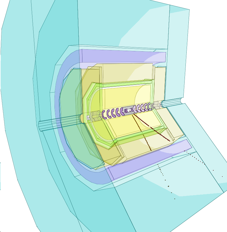
The naturalness-required light higgsinos may be produced at decent rates at LHC but their relatively compressed spectra imply low visible energy release from their decays. Thus, light higgsinos are very challenging to see at LHC [Baer:2014kya, Baer:2018hpb]. In contrast, the International Linear e+esuperscript𝑒superscript𝑒e^{+}e^{-} Collider (ILC) with s>2m(higgsino)𝑠2𝑚𝑖𝑔𝑔𝑠𝑖𝑛𝑜\sqrt{s}>2m(higgsino) would be a higgsino factory in addition to being a Higgs factory. The reactions e+eχ~1+χ~1superscript𝑒superscript𝑒superscriptsubscript~𝜒1superscriptsubscript~𝜒1e^{+}e^{-}\rightarrow\tilde{\chi}_{1}^{+}\tilde{\chi}_{1}^{-} and χ~20χ~10subscriptsuperscript~𝜒02subscriptsuperscript~𝜒01\tilde{\chi}^{0}_{2}\tilde{\chi}^{0}_{1} should occur at rates comparable to muon pair production and at rates exceeding Zh𝑍Zh production [Baer:2014yta]. The expected mass gaps mχ~1mχ~10mχ~20mχ~10320similar-tosubscript𝑚subscript~𝜒1subscript𝑚subscriptsuperscript~𝜒01subscript𝑚subscriptsuperscript~𝜒02subscript𝑚subscriptsuperscript~𝜒01similar-to320m_{\tilde{\chi}_{1}}-m_{\tilde{\chi}^{0}_{1}}\sim m_{\tilde{\chi}^{0}_{2}}-m_{\tilde{\chi}^{0}_{1}}\sim 3-20 GeV lead to events which are easily identified at ILC: see Fig. 1 for a simulated e+eχ~10χ~20superscript𝑒superscript𝑒subscriptsuperscript~𝜒01subscriptsuperscript~𝜒02e^{+}e^{-}\rightarrow\tilde{\chi}^{0}_{1}\tilde{\chi}^{0}_{2} with χ~20μ+μχ~10subscriptsuperscript~𝜒02superscript𝜇superscript𝜇subscriptsuperscript~𝜒01\tilde{\chi}^{0}_{2}\rightarrow\mu^{+}\mu^{-}\tilde{\chi}^{0}_{1} event display with light higgsinos in the ILD detector.
Refer to caption
Figure 1: ILD event display of a simulated e+eχ~10χ~20superscript𝑒superscript𝑒subscriptsuperscript~𝜒01subscriptsuperscript~𝜒02e^{+}e^{-}\rightarrow\tilde{\chi}^{0}_{1}\tilde{\chi}^{0}_{2} event with χ~20μ+μχ~10subscriptsuperscript~𝜒02superscript𝜇superscript𝜇subscriptsuperscript~𝜒01\tilde{\chi}^{0}_{2}\rightarrow\mu^{+}\mu^{-}\tilde{\chi}^{0}_{1}.

The cleanliness of ILC higgsino pair production events along with tunable beam energy and beam polarization should allow for a rich program of higgsino measurements. While the higgsino masses should be comparable to the superpotential μ𝜇\mu parameter, thus allowing for a determination of μ𝜇\mu, the higgsino mass splittings depend sensitively on the weak scale gaugino masses M1subscript𝑀1M_{1} (bino) and M2subscript𝑀2M_{2} (wino). Thus, precision measurements of mχ~1±subscript𝑚superscriptsubscript~𝜒1plus-or-minusm_{\tilde{\chi}_{1}^{\pm}} and mχ~1,20subscript𝑚subscriptsuperscript~𝜒012m_{\tilde{\chi}^{0}_{1,2}} should allow for an extraction of M1subscript𝑀1M_{1} and M2subscript𝑀2M_{2} to good precision. Once the soft breaking gaugino masses are known, then the physical masses of the heavier neutralinos and charginos can also be found. The fitted values of M1subscript𝑀1M_{1} and M2subscript𝑀2M_{2} can be extrapolated to high energies to test the hypothesis of gaugino mass unification. If gluinos are discovered at LHC, then M3subscript𝑀3M_{3} (gluino) may be extracted[Baer:2016wkz] and unification of all three gaugino masses may be tested.

In this paper, we first present in Sec. 2 two natural SUSY benchmark models labeled ILC1 and ILC2 that arise from the non-universal Higgs model (NUHM2)[nuhm2]. These models allow for μ𝜇\mu as an input parameter so that SUSY spectra with a low value of ΔEWsubscriptΔEW\Delta_{\rm EW} can easily be generated. The NUHM2 model incorporates gaugino mass unification so that under renormalization group (RG) evolution M1subscript𝑀1M_{1} and M2subscript𝑀2M_{2} should unify at the scale mGUT2×1016similar-to-or-equalssubscript𝑚GUT2superscript1016m_{\rm GUT}\simeq 2\times 10^{16} GeV. We also propose a natural generalized mirage mediation (nGMM) benchmark model which instead has gaugino mass unification at the mirage scale μmir=mGUTe8π2/α5×107subscript𝜇𝑚𝑖𝑟subscript𝑚GUTsuperscript𝑒8superscript𝜋2𝛼similar-to5superscript107\mu_{mir}=m_{\rm GUT}e^{-8\pi^{2}/\alpha}\sim 5\times 10^{7} GeV where α=4𝛼4\alpha=4 parametrizes the relative amounts of modulus-mediation versus anomaly-mediation in SUSY breaking. In this case, by determining the mirage unification scale μmirsubscript𝜇𝑚𝑖𝑟\mu_{mir}, ILC can measure the strength α𝛼\alpha of moduli- vs. anomaly-mediation. If the gaugino masses are extrapolated beyond the mirage scale to the GUT scale, then ILC can also indirectly measure the underlying gravitino mass m3/2subscript𝑚32m_{3/2} [Baer:2016hfa]! Thus, in such cases ILC would allow for a window into the nature of the laws of physics at energy scales far beyond s0.51similar-to𝑠0.51\sqrt{s}\sim 0.5-1 TeV.

All three benchmarks have been studied in a detailed, Geant4-based simulation of the ILD detector concept [ILD], which we introduce in Sec. 3. In Sec. 4, we present a detailed portrait of various higgsino pair production measurements at ILC with s=500𝑠500\sqrt{s}=500 GeV. Continuum measurements of energy and invariant mass distributions of higgsino decay products should allow for extraction of higgsino masses to percent level or better precision.

In Sec. 5, we present results from our calculations using the Fittino [64] program to extract fits of fundamental weak scale MSSM Lagrangian parameters, especially the gaugino masses M1subscript𝑀1M_{1} and M2subscript𝑀2M_{2}. We also obtain predictions for the masses of many of the kinematically inaccessible superparticles. We then can extract the underlying GUT scale parameters if we assume a particular high scale SUSY model such as NUHM2, NUHM3 or nGMM. If the gluino is discovered at LHC, the extracted gaugino masses may be augmented with the SU(3)𝑆𝑈3SU(3) gaugino mass M3subscript𝑀3M_{3}. We also show that the thermally-produced relic density of WIMPs may be extracted, thus testing the WIMP-only versus mixed axion-WIMP dark matter hypotheses. In Sec. 6, we show results from running the gaugino masses to high energy scales, thus offering a test of the unification hypothesis and the underlying SUSY breaking mechanism. A summary and conclusions are presented in Sec. 7.

2 Benchmark models

In this Section, we present three natural SUSY benchmark points which have been used for the detailed ILD studies described in Sec. 3 and Sec. 4.

2.1 ILC1 benchmark model

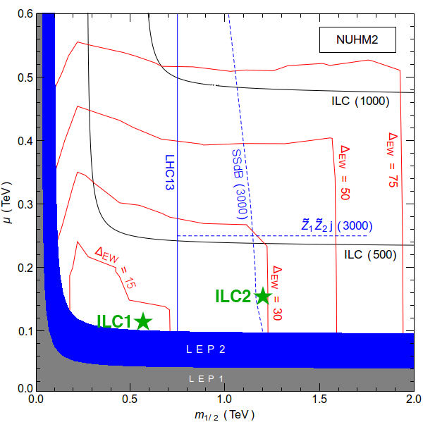
The ILC1 benchmark point, whose parameters are listed in Tab. 1, has been presented previously [Baer:2012up] and has been used for some detailed ILC studies using a toy detector simulation [Baer:2014yta]. The ILC1 benchmark point was generated within the NUHM2 model with input parameters and output masses as listed. While the various matter scalars are essentially decoupled for LHC and ILC physics, the spectrum does contain light higgsinos with mass mχ~1=117.3subscript𝑚subscript~𝜒1117.3m_{\tilde{\chi}_{1}}=117.3 GeV and mχ~1,20=102.7subscript𝑚subscriptsuperscript~𝜒012102.7m_{\tilde{\chi}^{0}_{1,2}}=102.7 and 124124124 GeV, respectively, so that higgsino pair production should already turn on for ILC with s>227𝑠227\sqrt{s}>227 GeV. The associated mass gaps, which play a central role in these analyses, are mχ~1±mχ~10=14.6subscript𝑚superscriptsubscript~𝜒1plus-or-minussubscript𝑚subscriptsuperscript~𝜒0114.6m_{\tilde{\chi}_{1}^{\pm}}-m_{\tilde{\chi}^{0}_{1}}=14.6 GeV and mχ~20mχ~10=21.3subscript𝑚subscriptsuperscript~𝜒02subscript𝑚subscriptsuperscript~𝜒0121.3m_{\tilde{\chi}^{0}_{2}}-m_{\tilde{\chi}^{0}_{1}}=21.3 GeV. The model contains a light Higgs scalar with mh=125.3subscript𝑚125.3m_{h}=125.3 GeV due to highly mixed TeV-scale top squarks with mt~1=1893.3subscript𝑚subscript~𝑡11893.3m_{\tilde{t}_{1}}=1893.3 GeV (well beyond the reach of HL-LHC [Baer:2012vr] where the 95% CL exclusion reach extends to mt~11400similar-tosubscript𝑚subscript~𝑡11400m_{\tilde{t}_{1}}\sim 1400 GeV [ATLAS:2013hta]). The model is highly electroweak natural with ΔEW=14subscriptΔEW14\Delta_{\rm EW}=14 corresponding to just 7% fine-tuning. This benchmark is now likely excluded by LHC: The gluino mass mg~=1563.5subscript𝑚~𝑔1563.5m_{\tilde{g}}=1563.5 GeV is excluded by LHC13 searches with 36similar-toabsent36\sim 36 fb-1. The searches for higgsinos with small mass-splittings performed by CMS  [Sirunyan:2018iwl] and ATLAS [Aaboud:2017leg] are done for a spectrum different from our benchmark - in particular the mass of χ~1±subscriptsuperscript~𝜒plus-or-minus1\tilde{\chi}^{\pm}_{1} is assumed to be exactly halfway between those of χ~10subscriptsuperscript~𝜒01\tilde{\chi}^{0}_{1} and χ~20subscriptsuperscript~𝜒02\tilde{\chi}^{0}_{2} - but are nevertheless likely to exclude it. However, we retain the point for comparison with previous work. If one adopts modest gaugino mass non-universality, then a small increase in M3(weak)>2subscript𝑀3𝑤𝑒𝑎𝑘2M_{3}(weak)>2 TeV would bring the point in accord with LHC searches. The relic density of thermally produced higgsino-like LSPs is a factor 13 below the measured value. Requiring also naturalness in the QCD sector, then one must bring the axion into the model, and axionic dark matter may constitute the bulk of the dark matter [Bae:2013bva]. The location of the ILC1 benchmark point is denoted by one of the green stars in the μ𝜇\mu vs. M1/2subscript𝑀12M_{1/2} parameter space plane of the NUHM2 model shown in Fig. 2.
Refer to caption
Figure 2: The M1/2subscript𝑀12M_{1/2} vs. μ𝜇\mu plane in the NUHM2 model for tanβ=15𝛽15\tan\beta=15, M0=5subscript𝑀05M_{0}=5 TeV, A0=8subscript𝐴08A_{0}=-8 TeV and MA=1subscript𝑀𝐴1M_{A}=1 TeV. We show contours of ΔEWsubscriptΔEW\Delta_{\rm EW} along with some limits from LHC13 and the future reach of ILC with s=500𝑠500\sqrt{s}=500 and 1000 GeV and HL-LHC (via same-sign diboson production labeled SSdB (3000) and via neutralino associated production labeled Z~1Z~2jsubscript~𝑍1subscript~𝑍2𝑗\widetilde{Z}_{1}\widetilde{Z}_{2}j (3000) in the nomenclature of Ref. [Baer:2016usl] where Z~isubscript~𝑍𝑖\widetilde{Z}_{i} denotes neutralino eigenstate i𝑖i). Location of benchmark points is indicated in green. To aid the reader, we note that mg~2.5M1/2similar-tosubscript𝑚~𝑔2.5subscript𝑀12m_{\tilde{g}}\sim 2.5\,M_{1/2}. The figure is adapted from Ref. [Baer:2016usl].
Table 1: Input parameters and mass spectrum and rates for benchmark points ILC1, ILC2 and nGMM1. All masses and dimensionful parameters are in GeV units. All values have been obtained with ISASUGRA.
units ILC1 ILC2 nGMM1
M0subscript𝑀0M_{0} [GeV] 7025.0 5000
M1/2subscript𝑀12M_{1/2} [GeV] 568.3 1200
A0subscript𝐴0A_{0} [GeV] -10427 -8000
m3/2subscript𝑚32m_{3/2} [GeV] 75000
M1,M2,M3subscript𝑀1subscript𝑀2subscript𝑀3M_{1},M_{2},M_{3} [GeV] 3382.5, 2124.4, 1225.8
tanβ𝛽\tan\beta 10 15 10
a3subscript𝑎3a_{3} 3
cmsubscript𝑐𝑚c_{m} 6.9
α𝛼\alpha 4
mhsubscript𝑚m_{h} [GeV] 125.3 125.4 124.9
mAsubscript𝑚𝐴m_{A} [GeV] 1000.0 1000 2000
mHsubscript𝑚𝐻m_{H} [GeV] 1006.8 1006.7 2013.3
mH±subscript𝑚superscript𝐻plus-or-minusm_{H^{\pm}} [GeV] 1003.2 1003.2 2001.6
μ𝜇\mu [GeV] 115.0 150 150
mg~subscript𝑚~𝑔m_{\tilde{g}} [GeV] 1563.5 2832.6 2856.5
mχ~1±subscript𝑚subscriptsuperscript~𝜒plus-or-minus1m_{\tilde{\chi}^{\pm}_{1}}, mχ~2±subscript𝑚subscriptsuperscript~𝜒plus-or-minus2m_{\tilde{\chi}^{\pm}_{2}} [GeV] 117.3, 513.0 158.3, 1017.5 158.7, 1791.6
mχ~10subscript𝑚subscriptsuperscript~𝜒01m_{\tilde{\chi}^{0}_{1}}, mχ~20subscript𝑚subscriptsuperscript~𝜒02m_{\tilde{\chi}^{0}_{2}} [GeV] 102.7, 124.0 148.1, 157.8 151.4, 155.8
mχ~30subscript𝑚subscriptsuperscript~𝜒03m_{\tilde{\chi}^{0}_{3}}, mχ~40subscript𝑚subscriptsuperscript~𝜒04m_{\tilde{\chi}^{0}_{4}} [GeV] 267.0, 524.2 538.7, 1031.1 1526.9, 1799.4
mu~Lsubscript𝑚subscript~𝑢𝐿m_{\tilde{u}_{L}}, mu~Rsubscript𝑚subscript~𝑢𝑅m_{\tilde{u}_{R}} [GeV] 7021, 7254 5440, 5566 5267, 5399
mt~1subscript𝑚subscript~𝑡1m_{\tilde{t}_{1}}, mt~2subscript𝑚subscript~𝑡2m_{\tilde{t}_{2}} [GeV] 1893, 4919 1774, 3878 1433, 3732
md~Lsubscript𝑚subscript~𝑑𝐿m_{\tilde{d}_{L}}, md~Rsubscript𝑚subscript~𝑑𝑅m_{\tilde{d}_{R}} [GeV] 7022, 6999 5441, 5384 5267, 5229
mb~1subscript𝑚subscript~𝑏1m_{\tilde{b}_{1}}, mb~2subscript𝑚subscript~𝑏2m_{\tilde{b}_{2}} [GeV] 4959, 6893 3903, 5204 3770, 5124
me~Lsubscript𝑚subscript~𝑒𝐿m_{\tilde{e}_{L}}, me~Rsubscript𝑚subscript~𝑒𝑅m_{\tilde{e}_{R}} [GeV] 7152, 6759 5149, 4817 5128, 4825
mτ~1subscript𝑚subscript~𝜏1m_{\tilde{\tau}_{1}}, mτ~2subscript𝑚subscript~𝜏2m_{\tilde{\tau}_{2}} [GeV] 6657, 7103 4652, 5072 4749, 5094
Ωχ~0TPh2superscriptsubscriptΩsuperscript~𝜒0TPsuperscript2\Omega_{\tilde{\chi}^{0}}^{\rm TP}h^{2} 0.009 0.007 0.005
σv(v0)delimited-⟨⟩𝜎𝑣𝑣0\langle\sigma v\rangle(v\rightarrow 0) [cm3 s-1] 2.2×1025absentsuperscript1025\times 10^{-25} 2.9×1025absentsuperscript1025\times 10^{-25} 3.1×1025absentsuperscript1025\times 10^{-25}
σSI(χ~0p)×109superscript𝜎SIsuperscript~𝜒0𝑝superscript109\sigma^{\rm SI}(\tilde{\chi}^{0}p)\times 10^{9} [pb] 6.8 1.5 0.3
aμSUSY×1010superscriptsubscript𝑎𝜇SUSYsuperscript1010a_{\mu}^{\rm SUSY}\times 10^{10} 0.03 0.13 0.06
BF(bsγ)×104𝐵𝐹𝑏𝑠𝛾superscript104BF(b\rightarrow s\gamma)\times 10^{4} 3.3 3.3 3.1
BF(BSμ+μ)×109𝐵𝐹subscript𝐵𝑆superscript𝜇superscript𝜇superscript109BF(B_{S}\rightarrow\mu^{+}\mu^{-})\times 10^{9} 3.8 3.8 3.8
BF(Buτντ)×104𝐵𝐹subscript𝐵𝑢𝜏subscript𝜈𝜏superscript104BF(B_{u}\rightarrow\tau\nu_{\tau})\times 10^{4} 1.3 1.3 1.3
ΔEWsubscriptΔEW\Delta_{\rm EW} 14 28 15
Table 2: Higgsino and gaugino fractions of the lightest neutralino χ~10superscriptsubscript~𝜒10\widetilde{\chi}_{1}^{0}. The fractions are expressed so that they satisfy the relation RH~2+RW~2+RB~2=1superscriptsubscript𝑅~𝐻2superscriptsubscript𝑅~𝑊2superscriptsubscript𝑅~𝐵21R_{\widetilde{H}}^{2}+R_{\widetilde{W}}^{2}+R_{\widetilde{B}}^{2}=1.
ILC1 ILC2 nGMM1
RH~subscript𝑅~𝐻R_{\widetilde{H}} 0.970.970.97 0.990.990.99 0.9990.9990.999
RW~subscript𝑅~𝑊R_{\widetilde{W}} 0.14-0.14-0.14 0.070.070.07 0.040.040.04
RB~subscript𝑅~𝐵R_{\widetilde{B}} 0.190.190.19 0.080.080.08 0.020.020.02

2.2 ILC2 benchmark

The ILC2 benchmark point is also generated within the NUHM2 SUSY model with parameter values as listed in Tab. 1. The location of ILC2 is indicated by the other green star in Fig. 2 and is found to lie just beyond the HL-LHC reach for the same-sign diboson signature arising from wino pair production [Baer:2013yha]. The higgsino pair signature from ppχ~10χ~20j𝑝𝑝subscriptsuperscript~𝜒01subscriptsuperscript~𝜒02𝑗pp\rightarrow\tilde{\chi}^{0}_{1}\tilde{\chi}^{0}_{2}j production followed by χ~20χ~10+subscriptsuperscript~𝜒02subscriptsuperscript~𝜒01superscriptsuperscript\tilde{\chi}^{0}_{2}\rightarrow\tilde{\chi}^{0}_{1}\ell^{+}\ell^{-} decay should be viable since the cluster of higgsinos lies in the vicinity of μ=150𝜇150\mu=150 GeV [Baer:2014kya]. The value of mg~=2832subscript𝑚~𝑔2832m_{\tilde{g}}=2832 GeV appears just beyond the HL-LHC reach for gluino pair production (where the 5σ5𝜎5\sigma reach extends to mg~2800similar-tosubscript𝑚~𝑔2800m_{\tilde{g}}\sim 2800 GeV[Baer:2016wkz]). The higher value of gaugino masses in ILC2 – as compared to benchmark point ILC1 – is reflected in the reduced inter-higgsino mass gaps where we find mχ~1mχ~10=10.2subscript𝑚subscript~𝜒1subscript𝑚subscriptsuperscript~𝜒0110.2m_{\tilde{\chi}_{1}}-m_{\tilde{\chi}^{0}_{1}}=10.2 GeV and mχ~20mχ~10=9.7subscript𝑚subscriptsuperscript~𝜒02subscript𝑚subscriptsuperscript~𝜒019.7m_{\tilde{\chi}^{0}_{2}}-m_{\tilde{\chi}^{0}_{1}}=9.7 GeV. The naturalness measure ΔEW=28subscriptΔEW28\Delta_{\rm EW}=28 leads to 3%similar-toabsentpercent3\sim 3\% electroweak fine-tuning. The thermally-produced abundance of dark matter Ωχ~10TPh20.007similar-tosuperscriptsubscriptΩsubscriptsuperscript~𝜒01TPsuperscript20.007\Omega_{\tilde{\chi}^{0}_{1}}^{\rm TP}h^{2}\sim 0.007, well below the measured value of 0.12. So, as for ILC1, the axions needed to solve the strong CP problem can be expected to make up the remainder.

2.3 Natural mirage mediation (NMM) benchmark

Mirage mediated (MM) SUSY breaking models are motivated by string model compactifications with moduli fields stabilized by fluxes and where an uplifted scalar potential leads to a de Sitter vacuum (as required by cosmology) with a small breaking of supersymmetry[Choi:2004sx, Choi:2005ge, Choi:2007ka]. In such cases, it is expected that the SUSY breaking soft terms arise with comparable moduli-mediated and anomaly-mediated contributions. In the gaugino sector (and in the scalar sector for particular modular weight choices) the GUT scale soft masses are offset from each other by contributions containing their gauge group beta functions. As a consequence, the running of the gaugino masses exactly compensates the high scale mass splitting leading to an apparent unification at the intermediate (mirage) scale μmir=mGUTe8π2/αsubscript𝜇𝑚𝑖𝑟subscript𝑚GUTsuperscript𝑒8superscript𝜋2𝛼\mu_{mir}=m_{\rm GUT}e^{-8\pi^{2}/\alpha} where the parameter α𝛼\alpha is introduced to parametrize the relative amounts of anomaly- versus moduli-mediation. A value α=0𝛼0\alpha=0 corresponds to pure anomaly-mediation (with tachyonic sleptons) while, as α𝛼\alpha gets large, the soft terms become increasingly universal.

Initially, simple MM models predicted scalar masses involving discrete values of scalar field modular weights which depend on the compactification geometry and upon which branes harbored the various visible sector fields. This class of models, over a wide range of choices for modular weights, was found to be unnatural when mh125similar-to-or-equalssubscript𝑚125m_{h}\simeq 125 GeV was required[Baer:2014ica]. However, in more general compactification and stabilization schemes, then the previously discrete parameter choices cmsubscript𝑐𝑚c_{m}, cHusubscript𝑐subscript𝐻𝑢c_{H_{u}}, cHdsubscript𝑐subscript𝐻𝑑c_{H_{d}} and a3subscript𝑎3a_{3} become continuous, allowing for the construction of models with low values of ΔEWsubscriptΔEW\Delta_{\rm EW}[Baer:2016hfa].

In Tab. 1, we show one such example point from natural generalized mirage mediation or nGMM in column 4. The gaugino masses unify at the mirage scale μmir5×107similar-tosubscript𝜇𝑚𝑖𝑟5superscript107\mu_{mir}\sim 5\times 10^{7} GeV. The rather large value of mg~=2856.5subscript𝑚~𝑔2856.5m_{\tilde{g}}=2856.5 GeV means the winos and bino are also rather massive so that both gluino pair production and wino pair production appear out of reach of HL-LHC. The higgsinos are clustered with masses around μ150similar-to𝜇150\mu\sim 150 GeV but with even smaller mass splittings than ILC2: mχ~1mχ~10=7.3subscript𝑚subscript~𝜒1subscript𝑚subscriptsuperscript~𝜒017.3m_{\tilde{\chi}_{1}}-m_{\tilde{\chi}^{0}_{1}}=7.3 GeV and mχ~20mχ~10=4.4subscript𝑚subscriptsuperscript~𝜒02subscript𝑚subscriptsuperscript~𝜒014.4m_{\tilde{\chi}^{0}_{2}}-m_{\tilde{\chi}^{0}_{1}}=4.4 GeV. Such small neutralino mass splittings may also push the soft dilepton plus jet signature from χ~10χ~20jsubscriptsuperscript~𝜒01subscriptsuperscript~𝜒02𝑗\tilde{\chi}^{0}_{1}\tilde{\chi}^{0}_{2}j production out of reach of HL-LHC [Baer:2018hpb]. Nonetheless, the model is highly natural with ΔEW=15subscriptΔEW15\Delta_{\rm EW}=15 or 6.7% fine-tuning. The LSP is more purely higgsino-like than the ILC1 or ILC2 benchmarks leading to a reduced thermally-produced dark matter relic density and reduced direct dark matter detection rates. Thus, direct detection of WIMP dark matter from the nGMM1 benchmark may require multi-ton noble liquid detectors for discovery.

3 Software Tools and Observables

In this section we describe the main features of the ILD detector as used for the simulation study and introduce the characteristics of the higgsino signal on which the strategies for event selection and reconstruction will be based.

3.1 Event generation

The physical masses for the three benchmark points have been calculated by ISASUGRA. The SUSY and SM events have been generated using WHIZARD 1.95 [Whizard], which considers both resonant and non-resonant production, as well as their interference. WHIZARD also generates the amount and spectrum of ISR appropriate for each considered channel, and takes beam-polarisation fully into account. The dedicated setup of the generator provided by the ILC Generator Group was used, and all types SM e+esuperscript𝑒superscript𝑒e^{+}e^{-} interactions yielding up to six fermions in the final state were considered. In addition, all eγ𝑒𝛾e\gamma interactions yielding three or five fermions and all γγ𝛾𝛾\gamma\gamma interactions yielding up to four fermions were also included. The initial photons in the latter cases might be virtual (in which case the beam remnants come in addition to the final fermions), or real from the photon component of the beams (in which case there is no beam remnants). The electron and positron beams have an initial energy-spread, which is further smeared by the effects of beamstrahlung. The resulting spectra as well as the flux and energy spectra of the beam photons are simulated according to the parameters in the ILC Technical Design Report (TDR) [TDR], using GuineaPig[Schulte:1999tx].

Pure left-handed or right-handed beam polarisations are used for the event generation. These samples are then weighted according to the nominal ILC beam polarisations for our simulation study. We introduce the following notation for beam polarizations, 𝒫(𝒫e,𝒫e+)𝒫subscript𝒫superscript𝑒subscript𝒫superscript𝑒\mathcal{P}\equiv(\mathcal{P}_{e^{-}},\mathcal{P}_{e^{+}}), and define the pure beam polarisations as 𝒫LR(1,+1)subscript𝒫𝐿𝑅11\mathcal{P}_{LR}\equiv(-1,+1) and 𝒫RL(+1,1)subscript𝒫𝑅𝐿11\mathcal{P}_{RL}\equiv(+1,-1). The nominal beam polarisations for the ILC are defined as 𝒫+(0.8,+0.3)subscript𝒫absent0.80.3\mathcal{P}_{-+}\equiv(-0.8,+0.3) and 𝒫+(+0.8,0.3)subscript𝒫absent0.80.3\mathcal{P}_{+-}\equiv(+0.8,-0.3).

Table 3 shows the production cross sections for chargino and neutralino pairs for the three benchmark models introduced in Sec. 2.1-2.3 for 100% polarised beams at several center-of-mass energies. Table 4 shows the decay branching ratios in the same three benchmarks.

The results of the simulation study assume a center-of-mass energy of s=500𝑠500\sqrt{s}=500 GeV and an integrated luminosity of =500500\mathcal{L}=500 fb-1 for each beam polarisation; these results are then scaled according to the operation scenarios listed in Tab. 5 for the parameter fit. In case of ILC1, where all three higgsinos would already be kinematically accessible at s=250𝑠250\sqrt{s}=250 GeV, the assumed integrated luminosities correspond to the H20 operating scenario, while for the other two benchmarks the I20 scenario was assumed, since in these cases the higgsinos are only accessible at s=350𝑠350\sqrt{s}=350 GeV.

Table 3: Chargino and neutralino production cross sections for the three benchmark points calculated using WHIZARD at various center-of-mass energies. The ILC beam energy spectrum and ISR effects are included. Pure beam polarizations are assumed.
Cross Section [fb]
s𝑠\sqrt{s} Process 𝒫𝒫\mathcal{P} ILC1 ILC2 nGMM1
250 GeV ee+χ~1+χ~1superscript𝑒superscript𝑒subscriptsuperscript~𝜒1subscriptsuperscript~𝜒1e^{-}e^{+}\rightarrow\widetilde{\chi}^{+}_{1}\widetilde{\chi}^{-}_{1} 𝒫LRsubscript𝒫𝐿𝑅\mathcal{P}_{LR} 2618
𝒫RLsubscript𝒫𝑅𝐿\mathcal{P}_{RL} 397.1
ee+χ~10χ~20superscript𝑒superscript𝑒subscriptsuperscript~𝜒01subscriptsuperscript~𝜒02e^{-}e^{+}\rightarrow\widetilde{\chi}^{0}_{1}\widetilde{\chi}^{0}_{2} 𝒫LRsubscript𝒫𝐿𝑅\mathcal{P}_{LR} 1044
𝒫RLsubscript𝒫𝑅𝐿\mathcal{P}_{RL} 804.8
350 GeV ee+χ~1+χ~1superscript𝑒superscript𝑒subscriptsuperscript~𝜒1subscriptsuperscript~𝜒1e^{-}e^{+}\rightarrow\widetilde{\chi}^{+}_{1}\widetilde{\chi}^{-}_{1} 𝒫LRsubscript𝒫𝐿𝑅\mathcal{P}_{LR} 3094 1602 1571
𝒫RLsubscript𝒫𝑅𝐿\mathcal{P}_{RL} 538.8 302.8 301.4
ee+χ~10χ~20superscript𝑒superscript𝑒subscriptsuperscript~𝜒01subscriptsuperscript~𝜒02e^{-}e^{+}\rightarrow\widetilde{\chi}^{0}_{1}\widetilde{\chi}^{0}_{2} 𝒫LRsubscript𝒫𝐿𝑅\mathcal{P}_{LR} 897.0 578.5 576.0
𝒫RLsubscript𝒫𝑅𝐿\mathcal{P}_{RL} 691.5 446.0 444.1
500 GeV ee+χ~1+χ~1superscript𝑒superscript𝑒subscriptsuperscript~𝜒1subscriptsuperscript~𝜒1e^{-}e^{+}\rightarrow\widetilde{\chi}^{+}_{1}\widetilde{\chi}^{-}_{1} 𝒫LRsubscript𝒫𝐿𝑅\mathcal{P}_{LR} 1801 1531 1520
𝒫RLsubscript𝒫𝑅𝐿\mathcal{P}_{RL} 334.8 307.2 309.2
ee+χ~10χ~20superscript𝑒superscript𝑒subscriptsuperscript~𝜒01subscriptsuperscript~𝜒02e^{-}e^{+}\rightarrow\widetilde{\chi}^{0}_{1}\widetilde{\chi}^{0}_{2} 𝒫LRsubscript𝒫𝐿𝑅\mathcal{P}_{LR} 491.4 458.9 463.3
𝒫RLsubscript𝒫𝑅𝐿\mathcal{P}_{RL} 379.8 353.8 357.1
Table 4: Chargino and neutralino decay branching ratios for the three benchmark points calculated using ISASUGRA. For the final-state leptons, only the electrons and muons are included (=e,μ𝑒𝜇\ell=e,\mu).
ILC1 ILC2 nGMM1
BR(χ~1+χ~10qq)𝐵𝑅subscriptsuperscript~𝜒1subscriptsuperscript~𝜒01𝑞superscript𝑞BR(\widetilde{\chi}^{+}_{1}\rightarrow\widetilde{\chi}^{0}_{1}qq^{\prime}) 67%percent\% 67%percent\% 66%percent\%
BR(χ~1+χ~10+ν)𝐵𝑅subscriptsuperscript~𝜒1subscriptsuperscript~𝜒01superscriptsubscript𝜈BR(\widetilde{\chi}^{+}_{1}\rightarrow\widetilde{\chi}^{0}_{1}\ell^{+}\nu_{\ell}) 22%percent\% 22%percent\% 22%percent\%
BR(χ~20χ~10qq)𝐵𝑅subscriptsuperscript~𝜒02subscriptsuperscript~𝜒01𝑞superscript𝑞BR(\widetilde{\chi}^{0}_{2}\rightarrow\widetilde{\chi}^{0}_{1}qq^{\prime}) 58%percent\% 63%percent\% 51%percent\%
BR(χ~20χ~10+)𝐵𝑅subscriptsuperscript~𝜒02subscriptsuperscript~𝜒01superscriptsuperscriptBR(\widetilde{\chi}^{0}_{2}\rightarrow\widetilde{\chi}^{0}_{1}\ell^{+}\ell^{-}) 7.4%percent\% 8.0%percent\% 7.5%percent\%
Table 5: Total integrated luminosities for various operation scenarios for the ILC [68]. H20 is assumed for ILC1, while I20 is assumed for ILC2 and nGMM1. See Ref. [68] for the assumed timelines and machine upgrades.
Scenario s𝑠\sqrt{s} [GeV] 𝒫𝒫\mathcal{P} \mathcal{L} [fb-1]
H20 250 𝒫+subscript𝒫absent\mathcal{P}_{-+} 900
𝒫+subscript𝒫absent\mathcal{P}_{+-} 900
350 𝒫+subscript𝒫absent\mathcal{P}_{-+} 90
𝒫+subscript𝒫absent\mathcal{P}_{+-} 90
500 𝒫+subscript𝒫absent\mathcal{P}_{-+} 1600
𝒫+subscript𝒫absent\mathcal{P}_{+-} 1600
I20 250 𝒫+subscript𝒫absent\mathcal{P}_{-+} 225
𝒫+subscript𝒫absent\mathcal{P}_{+-} 225
350 𝒫+subscript𝒫absent\mathcal{P}_{-+} 765
𝒫+subscript𝒫absent\mathcal{P}_{+-} 765
500 𝒫+subscript𝒫absent\mathcal{P}_{-+} 1600
𝒫+subscript𝒫absent\mathcal{P}_{+-} 1600

3.2 The ILD detector model

The ILD concept is one of the two detectors being designed for the ILC. ILD employs a hybrid tracking system comprised of a time projection chamber and silicon strip sensors for tracking, and silicon pixel sensors as vertex detectors. Outside of the tracking system sits a highly granular calorimeter system optimized for particle flow reconstruction. A superconducting solenoid with a magnetic field of 3.53.53.5 T encases the calorimeters. An iron yoke outside the solenoid coil returns the magnetic flux, and is instrumented with scintillator-based muon detectors. In the low angle region, charged particles will be efficiently tracked down to 7 degrees. Dedicated calorimeters are placed in the forward region for detecting particles at even lower angles to the beam [Abramowicz:2010bg]. The most forward component of this system - the BeamCal - has holes for the beam-pipe, which constitutes the only region outside detector acceptance, and corresponds to 5.65.65.6 mrad.

The simulation and reconstruction tools used in this study are part of the iLCSoft framework (v01-16-02) [ILCSOFT]. The beam crossing angle of 141414 mrad and the response of the ILD detector in its version ILD_o1_v05 as used for the ILC TDR [ILD] are simulated using Mokka [Mokka] based on GEANT4. The event reconstruction is performed using the Marlin [Marlin] framework, including the particle flow algorithm PandoraPFA [Pandora] for calorimeter clustering and the analysis of track and calorimeter information.

3.3 Signal processes and key observables

We study the pair production of the two light charginos (χ~1+subscriptsuperscript~𝜒1\widetilde{\chi}^{+}_{1}, χ~1subscriptsuperscript~𝜒1\widetilde{\chi}^{-}_{1}) and two light neutralinos (χ~10subscriptsuperscript~𝜒01\widetilde{\chi}^{0}_{1}, χ~20subscriptsuperscript~𝜒02\widetilde{\chi}^{0}_{2}). In our benchmark models, the higgsino component is strongly dominant for these four light states. Their masses are shown in Tab. 1. The charginos and neutralinos are both produced dominantly via the s𝑠s-channel exchange since the sleptons are assumed to be heavy. The chargino pair production proceeds as e+eχ~1+χ~1superscript𝑒superscript𝑒subscriptsuperscript~𝜒1subscriptsuperscript~𝜒1e^{+}e^{-}\rightarrow\widetilde{\chi}^{+}_{1}\widetilde{\chi}^{-}_{1} through γ/Z𝛾𝑍\gamma/Z exchange, while the neutralino associated production e+eχ~10χ~20superscript𝑒superscript𝑒subscriptsuperscript~𝜒01subscriptsuperscript~𝜒02e^{+}e^{-}\rightarrow\widetilde{\chi}^{0}_{1}\widetilde{\chi}^{0}_{2} undergoes via the Z𝑍Z boson exchange. While in a real analysis at ILC more decay modes of the χ~20superscriptsubscript~𝜒20\widetilde{\chi}_{2}^{0} and the χ~1±superscriptsubscript~𝜒1plus-or-minus\widetilde{\chi}_{1}^{\pm} can be utilized, we focus here on the semi-leptonic channel for the charginos, i.e. χ~1+χ~1qq¯χ~10lνχ~10superscriptsubscript~𝜒1superscriptsubscript~𝜒1𝑞superscript¯𝑞superscriptsubscript~𝜒10𝑙𝜈superscriptsubscript~𝜒10\widetilde{\chi}_{1}^{+}\widetilde{\chi}_{1}^{-}\rightarrow q\bar{q}^{\prime}\widetilde{\chi}_{1}^{0}l\nu\widetilde{\chi}_{1}^{0}, and on the leptonic channel for the neutralinos, i.e. χ~20χ~10l+lχ~10superscriptsubscript~𝜒20superscriptsubscript~𝜒10superscript𝑙superscript𝑙superscriptsubscript~𝜒10\widetilde{\chi}_{2}^{0}\widetilde{\chi}_{1}^{0}\rightarrow l^{+}l^{-}\widetilde{\chi}_{1}^{0}. We restrict l=e,μ𝑙𝑒𝜇l=e,\mu in this study.

The key target observables are the three masses (Mχ~10subscript𝑀superscriptsubscript~𝜒10M_{\widetilde{\chi}_{1}^{0}}, Mχ~20subscript𝑀superscriptsubscript~𝜒20M_{\widetilde{\chi}_{2}^{0}}, and Mχ~1±subscript𝑀superscriptsubscript~𝜒1plus-or-minusM_{\widetilde{\chi}_{1}^{\pm}}) and, in this study, four polarized cross sections: chargino and neutralino production for the two opposite-sign beam polarization configurations. In a real ILC analysis, the like-sign combinations would be included as well, at least to serve as background-enriched control samples.

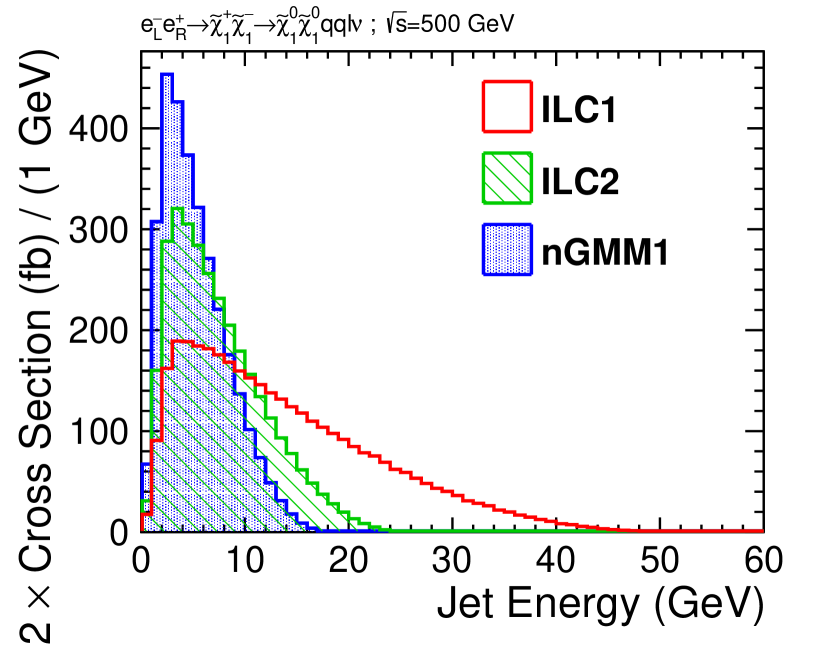
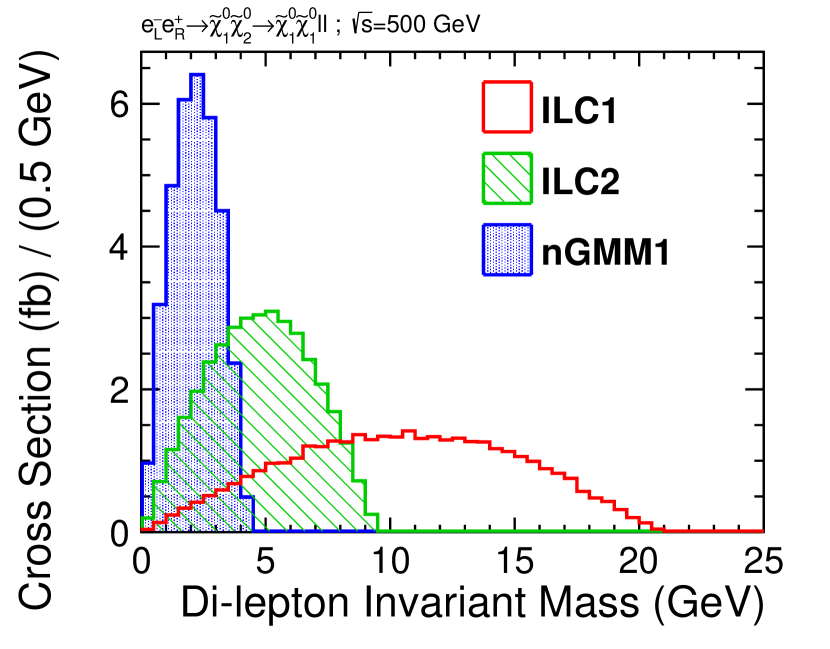
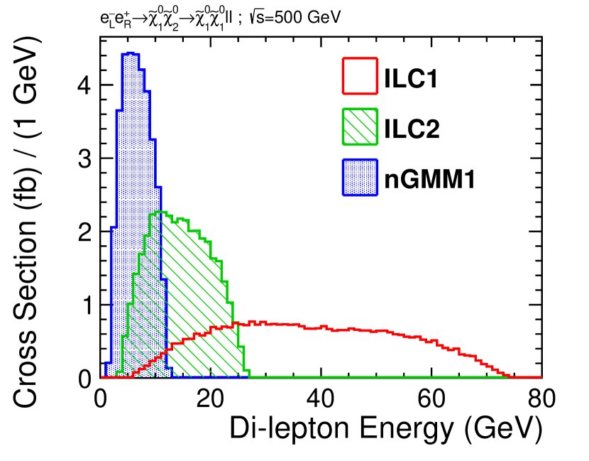
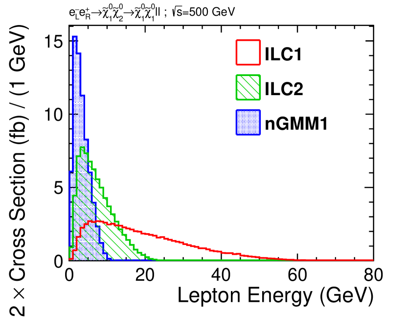
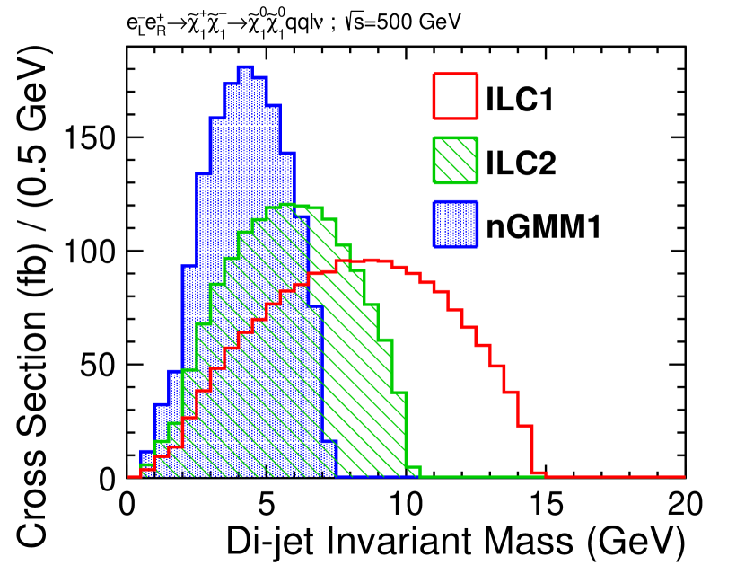
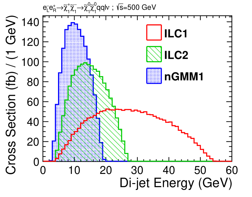
The three masses can be extracted from the maximum endpoints of the kinematic distributions shown at generator-level in Fig. 3(a),(b),(d) and (e). Specifically, we will rely on the maximum invariant mass and energy of the visible decay products of the χ~20l+lχ~10superscriptsubscript~𝜒20superscript𝑙superscript𝑙superscriptsubscript~𝜒10\widetilde{\chi}_{2}^{0}\rightarrow l^{+}l^{-}\widetilde{\chi}_{1}^{0} and χ~1±qq¯χ~10superscriptsubscript~𝜒1plus-or-minus𝑞superscript¯𝑞superscriptsubscript~𝜒10\widetilde{\chi}_{1}^{\pm}\rightarrow q\bar{q}^{\prime}\widetilde{\chi}_{1}^{0}. We find that the minimum endpoints, typically used in other SUSY studies, are too small to be useful in this study, since the resulting detector response is challenging to model in the soft spectrum and, in the case of the neutralino channel, it has large overlap with irreducible backgrounds.

The maximum energy Emaxsubscript𝐸maxE_{\mathrm{max}} of the di-jet (or di-lepton) system seen in the laboratory frame is given by444 The value for Emaxsubscript𝐸maxE_{\mathrm{max}} given in formula Eq. 2 is attained when the dilepton or dijet invariant mass is zero. The complete formulae relating the maximum and minimum energy to the invariant mass may be found on p. 439 of Ref. [Baer:2006rs]. The sensitivity of the analysis could even be improved by evaluating the maximum energy on an event-by-event basis, taking into account the dijet / dilepton invariant mass measured in each event individually.

Emax=γ(1+β)2(1+MM)ΔM,subscript𝐸max𝛾1𝛽21𝑀superscript𝑀Δ𝑀E_{\mathrm{max}}=\frac{\gamma(1+\beta)}{2}\left(1+\frac{M}{M^{\prime}}\right)\Delta M, (2)

where M𝑀M is the LSP (χ~10superscriptsubscript~𝜒10\widetilde{\chi}_{1}^{0}) mass and Msuperscript𝑀M^{\prime} is the mass of χ~1±superscriptsubscript~𝜒1plus-or-minus\widetilde{\chi}_{1}^{\pm} (χ~20superscriptsubscript~𝜒20\widetilde{\chi}_{2}^{0}) for the chargino (neutralino) channel. The mass difference is given by ΔM=MMΔ𝑀superscript𝑀𝑀\Delta M=M^{\prime}-M. As the decays studied are three body decays, it follows that the Lorentz-invariant mass of any pair of final-state particles has a maximum equal to the mass-difference between the decaying particle and the mass of the third decay product, see e.g. sect. 47.4.4.1 of [Tanabashi:2018oca]. In other words, the maximum of the the di-jet (or di-lepton) mass is a direct measure of ΔMΔ𝑀\Delta M. The boost factors β𝛽\beta and γ𝛾\gamma are given according to γ=(1β2)12𝛾superscript1superscript𝛽212\gamma=(1-\beta^{2})^{-\frac{1}{2}} and β=pM2+p2𝛽𝑝superscript𝑀2superscript𝑝2\beta=\frac{p}{\sqrt{M^{\prime 2}+p^{2}}}, where the maximum momentum p𝑝p in the laboratory frame is given by:

p=s212[(Ms)2+(Ms)2]+[(Ms)2(Ms)2]2.𝑝𝑠212delimited-[]superscript𝑀𝑠2superscriptsuperscript𝑀𝑠2superscriptdelimited-[]superscriptsuperscript𝑀𝑠2superscript𝑀𝑠22p=\frac{\sqrt{s}}{2}\sqrt{1-2\left[\left(\frac{M}{\sqrt{s}}\right)^{2}+\left(\frac{M^{\prime}}{\sqrt{s}}\right)^{2}\right]+\left[\left(\frac{M^{\prime}}{\sqrt{s}}\right)^{2}-\left(\frac{M}{\sqrt{s}}\right)^{2}\right]^{2}}. (3)

For any given channel, the measurements of ΔMΔ𝑀\Delta M and E𝐸E yield the masses M𝑀M and Msuperscript𝑀M^{\prime} by numerically solving the relations above. In our study, we obtain several measurements of ΔMΔ𝑀\Delta M and E𝐸E, specifically for the two different lepton final states (=e𝑒\ell=e and μ𝜇\mu), and for the two different beam polarizations 𝒫+subscript𝒫absent\mathcal{P}_{-+} and 𝒫+subscript𝒫absent\mathcal{P}_{+-}. These measurements can be readily combined individually for the chargino and neutralino channels. Because the chargino and neutralino measurements both include the LSP mass Mχ~10subscript𝑀superscriptsubscript~𝜒10M_{\widetilde{\chi}_{1}^{0}} in the observables, a final combination is performed using a fit to extract the uncertainty of the three masses.
Refer to caption
(a) chargino channel
Refer to caption
(b) chargino channel
Refer to caption
(c) chargino channel
Refer to caption
(d) neutralino channel
Refer to caption
(e) neutralino channel
Refer to caption
(f) neutralino channel
Figure 3: Generator-level distributions, given for the beam polarization with 𝒫LRsubscript𝒫𝐿𝑅\mathcal{P}_{LR}. The distributions for the other beam polarization 𝒫RLsubscript𝒫𝑅𝐿\mathcal{P}_{RL} are similar, up to the normalization due to the cross section.

Figure 3 shows the generator-level distributions of the mass and energy distributions for the di-jet (di-lepton) system for the chargino (neutralino) channel. The three benchmark points, ILC1, ILC2, and nGMM1, give progressively softer distributions due to the smaller mass gaps. The visible part of the chargino/neutralino decay will be very soft; for example, most of the jets and leptons have energies less than 20 GeV in the case of the ILC2 benchmark, and less than 10-15 GeV in the case of the nGMM1 benchmark.

3.4 Parameter Fitting

In the final step of the study we investigate the possibility to extract SUSY parameters from the projected measurement precisions obtained from the detector simulation. This will be addressed using a Markov chain technique as implemented in the program Fittino. Unless stated otherwise, the length of the Markov chains is 106superscript10610^{6} for each fitted configuration. While the MC samples used in the full detector simulation were based on Isajet, Fittino employs SPheno as a spectrum calculator during the fit. More details about the fitting procedure can be found in [66].

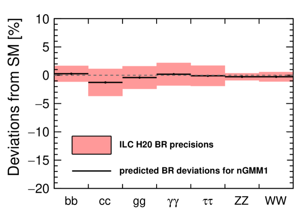
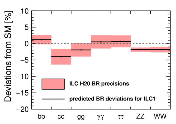
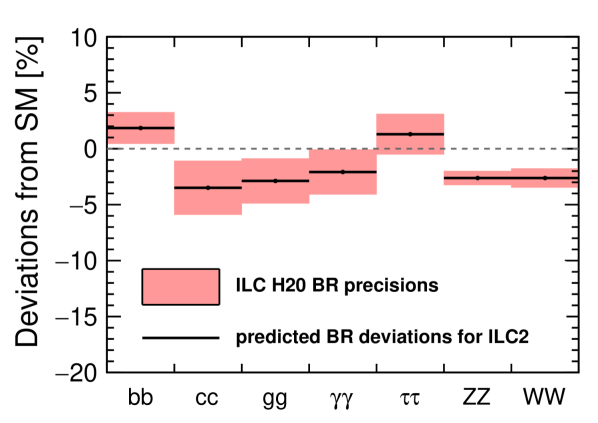
In addition to the mass and cross-section projections from this study, which will be described in detail in Sec. 4, a standard set of projected Higgs precision observables from the ILC was used to constrain the fit: These projections assume the H20 running scenario for the ILC [68], and include the Higgs mass (with a precision of 15 MeV as obtained in a ILD full simulation study [69]), and a set of Higgs branching ratio precisions obtained from the model-independent coupling fit results in [67], based on the so-called κ𝜅\kappa-framework.555Note that this includes the cross section measurements which in effect dominate the coupling precisions for the weak gauge bosons. For technical reasons the coupling precisions could not be used directly in the fit. The resulting precisions are shown in Fig. 4 in comparison to the expected deviations from the SM branching ratios in our three benchmarks. The Higgs mass and branching-ratio values are taken from FeynHiggs2.10.4 [bib:feynhiggs] for each of the SUSY models in question. For the NUHM2-based benchmarks, the most significant deviations would be observed in the Higgs couplings to the W𝑊W and Z𝑍Z bosons, although they would be hardly convincing as a discovery on their own. In case of nGMM1, all Higgs precision measurements agree perfectly with the SM.
Refer to caption
(a) ILC1
Refer to caption
(b) ILC2
Refer to caption
(c) nGMM1
Figure 4: Deviations of the branching fractions of the SUSY light Higgs from the Standard Model expectations, as obtained with FeynHiggs2.10.4. The uncertainty bands illustrate the expected measurement precisions after the full 250 and 500 GeV ILC program, assuming the H20 scenario [67]. Note that these are somewhat more conservative than the most recent estimates from [78].

4 Full Detector Simulation Study

For each benchmark point, we select separately the chargino and neutralino channels. These are considered as background to each other, including all decay modes. A common event selection is performed and provides sufficient sensitivity in all three benchmark cases. In a real experiment, once a signal has been discovered, the selection could be optimized based on initial mass estimates, see e.g. [54] for a discussion of how to boot-strap a selection of an a priori unknown signal. In the following sections, we describe the event selection for the chargino and neutralino channels.

4.1 Chargino channel

For the chargino pair production, we study the semileptonic final state ee+χ~1+χ~1χ~10χ~10qqνsuperscript𝑒superscript𝑒subscriptsuperscript~𝜒1subscriptsuperscript~𝜒1subscriptsuperscript~𝜒01subscriptsuperscript~𝜒01𝑞superscript𝑞subscript𝜈e^{-}e^{+}\rightarrow\widetilde{\chi}^{+}_{1}\widetilde{\chi}^{-}_{1}\rightarrow\widetilde{\chi}^{0}_{1}\widetilde{\chi}^{0}_{1}qq^{\prime}\ell\nu_{\ell} where =e𝑒\ell=e or μ𝜇\mu. The strategy here is to look for a single isolated lepton accompanied by two jets and large missing energy. We reconstruct the invariant mass and energy distributions of the di-jet system and extract their endpoints.

First, an isolated lepton candidate is identified according to the following criteria. Electron identification requires that the total energy measured in the calorimetric system Etotsubscript𝐸totE_{\rm tot} is consistent with the momentum measured in the tracker ptrksubscript𝑝trkp_{\rm trk}, such that they satisfy 0.5<Etot/ptrk<1.30.5subscript𝐸totsubscript𝑝trk1.30.5<E_{\rm tot}/p_{\rm trk}<1.3. In addition, the ECAL energy deposit EECALsubscript𝐸ECALE_{\rm ECAL} must be dominant over the HCAL energy deposit EHCALsubscript𝐸HCALE_{\rm HCAL}, so that we have EECAL/(EECAL+EHCAL)>0.9subscript𝐸ECALsubscript𝐸ECALsubscript𝐸HCAL0.9E_{\rm ECAL}/(E_{\rm ECAL}+E_{\rm HCAL})>0.9. For muon identification, we require that a charged track is associated with signals in the muon detector. In addition, lepton candidates with large impact parameter significance (>>5σ𝜎\sigma) are rejected in order to suppress backgrounds due to τ𝜏\tau or heavy quark decays. For the isolation requirement, we define an isolation cone around the lepton candidate with half-angle α𝛼\alpha such that cosα=0.95𝛼0.95\cos\alpha=0.95. We require that the total energy of charged particles within the cone (not including the candidate itself) is less than 0.2 GeV. The isolated lepton candidate with the highest transverse momentum is selected as the isolated lepton in the event.

Next, we deal with high cross section γγ𝛾𝛾\gamma\gamma processes that produce soft hadrons that overlap with our signal. Jet finders are used in two steps, following the procedures in [ILD]. We apply the ktsubscript𝑘𝑡k_{t} jet finder algorithm with the jet radius parameter R=1.4𝑅1.4R=1.4, forcing all reconstructed particles of the event apart from the isolated lepton into two jets, plus two additional beam jets; particles that are clustered into the beam jets are removed in the remainder of the event reconstruction [Catani:1993hr, Ellis:1993tq]. The value R=1.4𝑅1.4R=1.4 was chosen to yield dijet mass distributions which are optimal for the extraction of the kinematic endpoint. The remaining particles are used to reconstruct the chargino that decayed hadronically. They are forced into two jets using the Durham jet finding algorithm [Catani:1991hj].

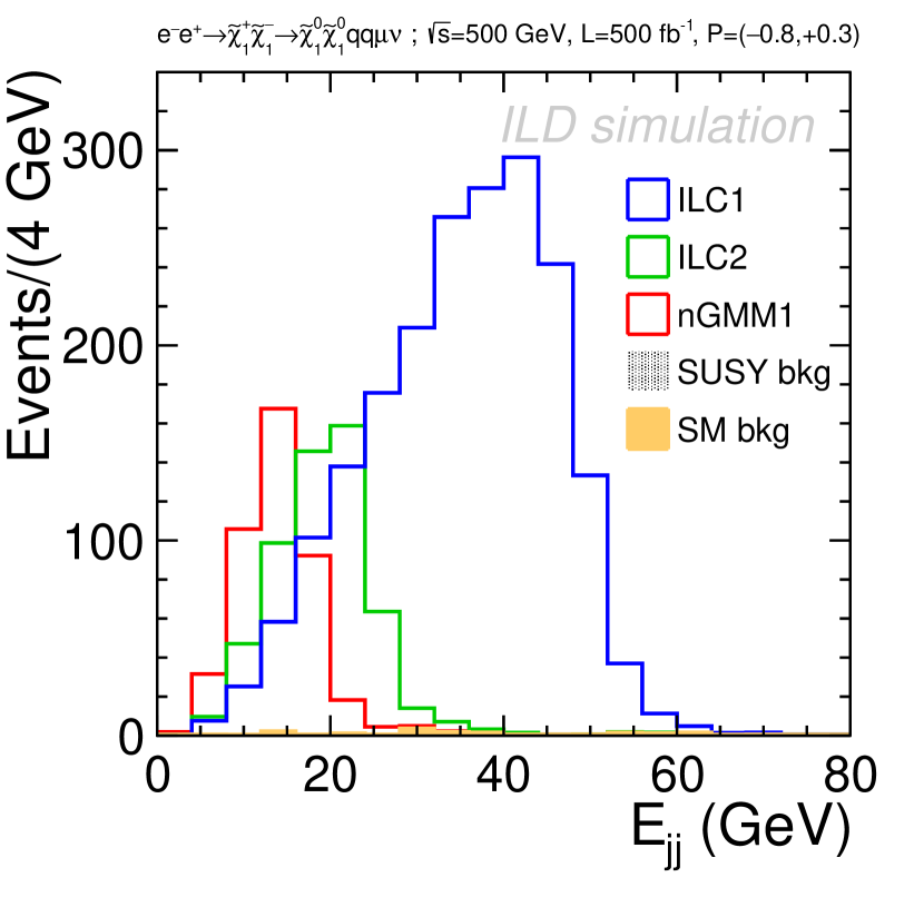
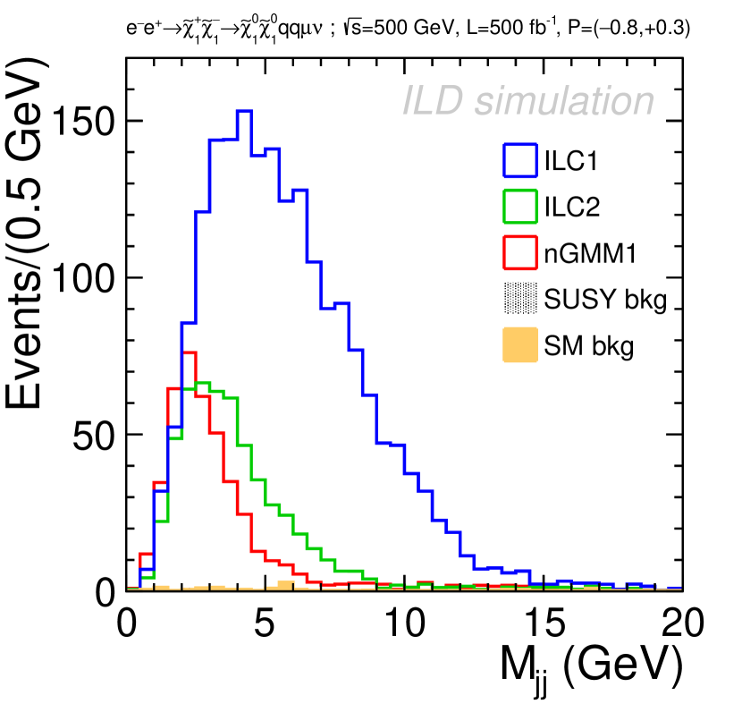
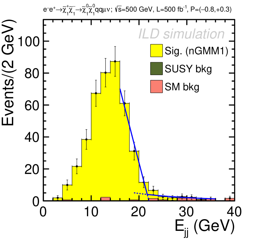
The event selection proceeds as follows. We select events with exactly one isolated lepton candidate, and its lepton type is identified. We reject events containing particles that are reconstructed in the BeamCal [Abramowicz:2010bg]. The transverse momentum of the lepton is required to be 5 GeV or greater. The number of reconstructed charged particles in each jet must be 2 or greater. It was tested whether a tighter cut on the track multiplicity would help to reject background from e.g. 3-prong τ𝜏\tau decays, but due to low jet energies, especially in the ILC2 and nGMM1 benchmarks, c.f.  Fig. 3(c), the resulting loss in signal was too severe. Both of the reconstructed jets should not be very forward, so that the polar angle of each jet θjsubscript𝜃𝑗\theta_{j} is such that |cosθj|<0.98subscript𝜃𝑗0.98|\cos\theta_{j}|<0.98. We require the coplanarity of the two jets as defined by the difference of the azimuthal angle to be Δϕ=|ϕ2ϕ1|<1.0Δitalic-ϕsubscriptitalic-ϕ2subscriptitalic-ϕ11.0\Delta\phi=|\phi_{2}-\phi_{1}|<1.0. The angle between the two jets θjjsubscript𝜃𝑗𝑗\theta_{jj} is required to satisfy |cosθjj|<0.2subscript𝜃𝑗𝑗0.2|\cos\theta_{jj}|<0.2. The visible energy in the event is required to be less than 80 GeV. The missing energy in the event is required to be greater than 400 GeV. The polar angle of the missing momentum θmisssubscript𝜃miss\theta_{\rm miss} is required to satisfy |cosθmiss|<0.99subscript𝜃miss0.99|\cos\theta_{\rm miss}|<0.99. The expected number of signal and background events after the event selection is shown in Tab. 6. Very few background events survive after the event selection. An example of the resulting distributions is shown for the qqμν𝑞𝑞𝜇𝜈qq\mu\nu channel with beam polarization 𝒫+subscript𝒫absent\mathcal{P}_{-+} in Fig. 5. The number of events at various steps of the event selection and the distributions for all studied channels can be found in Appendix A.

Table 6: Expected number of events after the event selction for the chargino signal and major backgrounds, normalized to an integrated luminosity of 500 fb-1. For each benchmark model the SUSY background is given in the column “Bkg.”.
e+eχ~1+χ~1superscript𝑒superscript𝑒subscriptsuperscript~𝜒1subscriptsuperscript~𝜒1e^{+}e^{-}\rightarrow\widetilde{\chi}^{+}_{1}\widetilde{\chi}^{-}_{1} ILC1 ILC2 nGMM1 SM bkg.
Process 𝒫𝒫\mathcal{P} Sig. Bkg. Sig. Bkg. Sig. Bkg. e+esuperscript𝑒superscript𝑒absente^{+}e^{-}\rightarrow 2f e+esuperscript𝑒superscript𝑒absente^{+}e^{-}\rightarrow 4f γγ𝛾𝛾absent\gamma\gamma\rightarrow 2f eγ𝑒𝛾absente\gamma\rightarrow 3f γγ𝛾𝛾absent\gamma\gamma\rightarrow 4f
qqeν𝑞𝑞𝑒𝜈qqe\nu 𝒫+subscript𝒫absent\mathcal{P}_{-+} 1463 85 392 23 283 15 5.9 64 0.0 22 2.0
𝒫+subscript𝒫absent\mathcal{P}_{+-} 404 23 96 4.6 73 5.1 7.4 16 0.0 8.0 2.0
qqμν𝑞𝑞𝜇𝜈qq\mu\nu 𝒫+subscript𝒫absent\mathcal{P}_{-+} 1862 108 509 28 389 29 33 37 0.0 0.0 7.0
𝒫+subscript𝒫absent\mathcal{P}_{+-} 524 34 127 8.5 101 8.2 8.2 7.2 0.0 0.0 7.0
Refer to caption
(a) di-jet energy
Refer to caption
(b) di-jet mass
Figure 5: Example of reconstructed distributions in the chargino channel e+eχ~1+χ~1χ~10χ~10qq¯μνμsuperscript𝑒superscript𝑒superscriptsubscript~𝜒1superscriptsubscript~𝜒1superscriptsubscript~𝜒10superscriptsubscript~𝜒10𝑞superscript¯𝑞𝜇subscript𝜈𝜇e^{+}e^{-}\rightarrow\tilde{\chi}_{1}^{+}\tilde{\chi}_{1}^{-}\rightarrow\tilde{\chi}_{1}^{0}\tilde{\chi}_{1}^{0}q\bar{q}^{\prime}\mu\nu_{\mu} with beam polarization 𝒫+subscript𝒫absent\mathcal{P}_{-+}. The contributions from SUSY and SM backgrounds are very small. The signal histograms are stacked on top of the backgrounds.
Refer to caption
(a) ILC1
Refer to caption
(b) ILC2
Refer to caption
(c) nGMM1
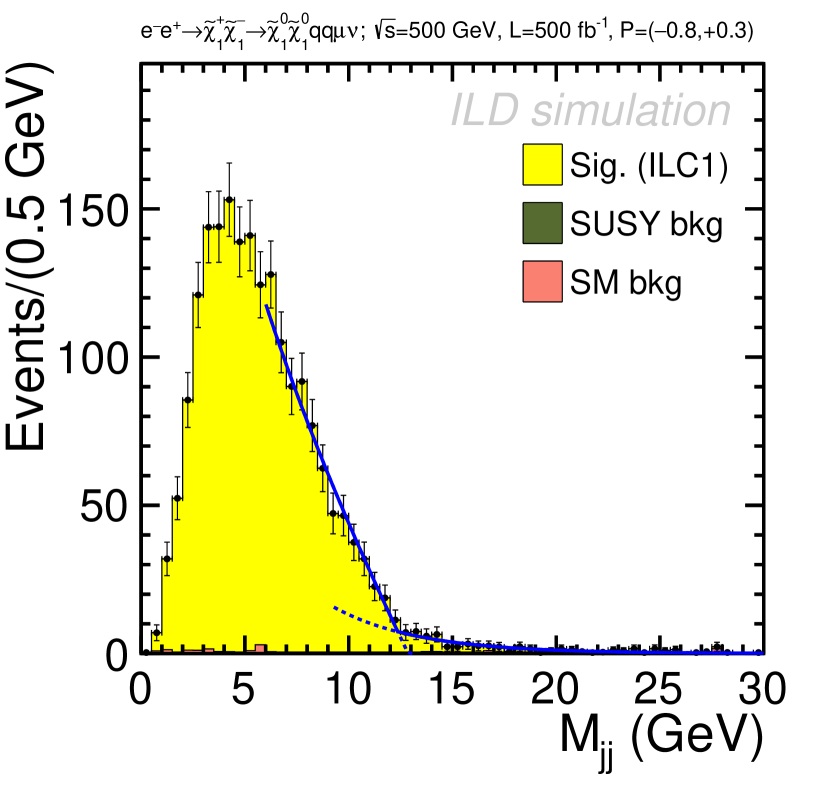
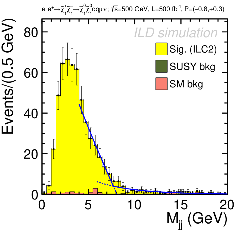
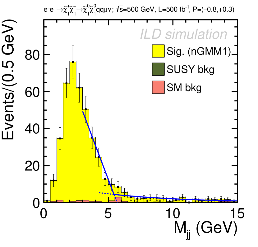
Figure 6: Example of the endpoint extraction of the di-jet invariant mass system in the chargino channel ee+χ~1+χ~1χ~10χ~10qq¯μνμsuperscript𝑒superscript𝑒superscriptsubscript~𝜒1superscriptsubscript~𝜒1superscriptsubscript~𝜒10superscriptsubscript~𝜒10𝑞superscript¯𝑞𝜇subscript𝜈𝜇e^{-}e^{+}\rightarrow\tilde{\chi}_{1}^{+}\tilde{\chi}_{1}^{-}\rightarrow\tilde{\chi}_{1}^{0}\tilde{\chi}_{1}^{0}q\bar{q}^{\prime}\mu\nu_{\mu} with beam polarization 𝒫+subscript𝒫absent\mathcal{P}_{-+} for the three benchmarks.
Refer to caption
(a) ILC1
Refer to caption
(b) ILC2
Refer to caption
(c) nGMM1
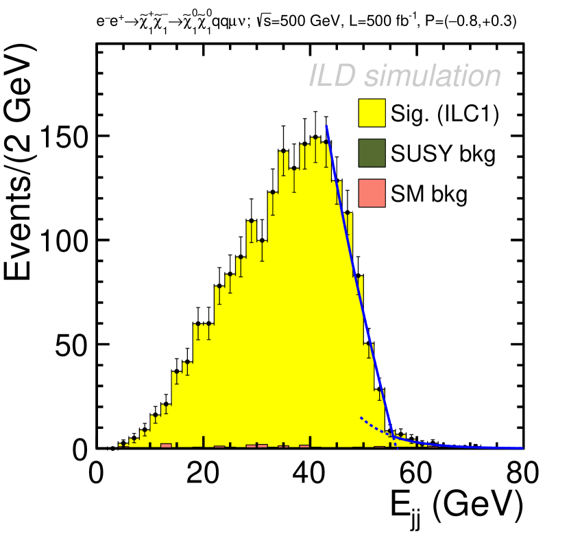
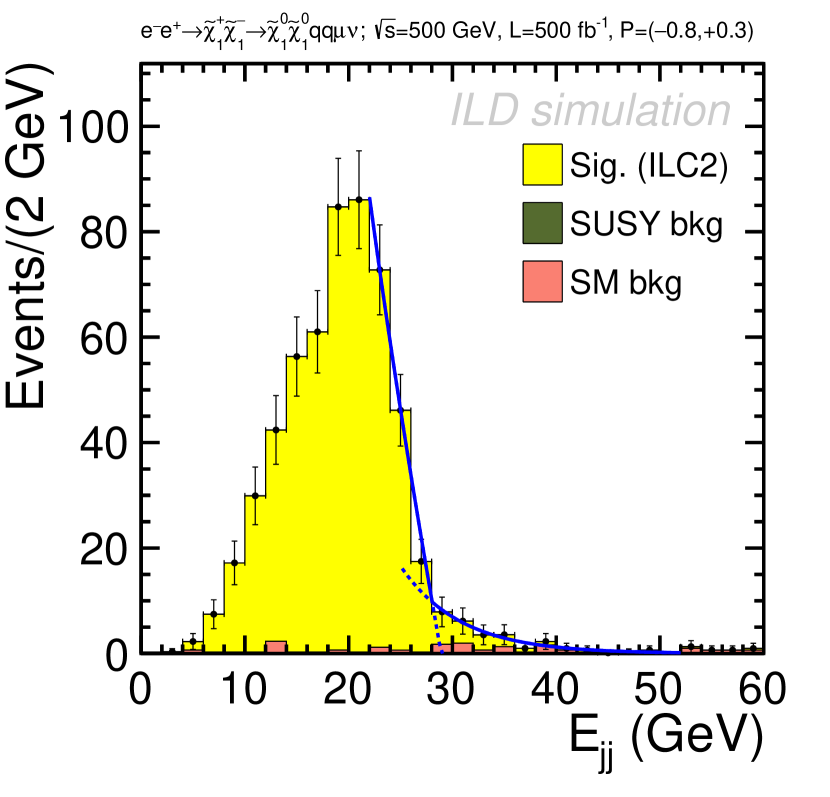
Figure 7: Example of the endpoint extraction of the di-jet energy system in the chargino channel ee+χ~1+χ~1χ~10χ~10qq¯μνμsuperscript𝑒superscript𝑒superscriptsubscript~𝜒1superscriptsubscript~𝜒1superscriptsubscript~𝜒10superscriptsubscript~𝜒10𝑞superscript¯𝑞𝜇subscript𝜈𝜇e^{-}e^{+}\rightarrow\tilde{\chi}_{1}^{+}\tilde{\chi}_{1}^{-}\rightarrow\tilde{\chi}_{1}^{0}\tilde{\chi}_{1}^{0}q\bar{q}^{\prime}\mu\nu_{\mu} with beam polarization 𝒫+subscript𝒫absent\mathcal{P}_{-+} for the three benchmarks.

The maximum endpoints of the dijet energy (Ejjsubscript𝐸𝑗𝑗E_{jj}) and mass (Mjjsubscript𝑀𝑗𝑗M_{jj}) distributions are extracted using a fit. Figures 7-6 show some examples of such a fit. Although the samples are almost free of backgrounds, the signal distribution has a tail which is caused by the failure to properly reconstruct the energy of soft neutral particles. We use an exponential curve to model such an effect, combined with a linear function to model the steep drop leading to the kinematic endpoint. The point where the two functions meet after the fit was used to estimate the kinematic endpoint. The statistical uncertainty of this value is estimated by performing toy Monte-Carlo experiments that repeatedly fit statistically fluctuated versions of these parent distributions. The extracted maximum endpoint of the dijet mass distributions is seen to have a systematic shift from the actual mass difference, which requires a correction at the level of 10-20% before they are used input to the final fit for the masses. It is assumed here that such a calibration procedure does not add any significant systematic uncertainties to our results, as described in [63]. The endpoints from the dijet energy distributions are used without corrections in the mass fit.

4.2 Neutralino channel

For the neutralino mixed production, we choose the clean leptonic decay of χ~20superscriptsubscript~𝜒20\widetilde{\chi}_{2}^{0} as the final state: ee+χ~10χ~20χ~10χ~10+superscript𝑒superscript𝑒subscriptsuperscript~𝜒01subscriptsuperscript~𝜒02subscriptsuperscript~𝜒01subscriptsuperscript~𝜒01superscriptsuperscripte^{-}e^{+}\rightarrow\widetilde{\chi}^{0}_{1}\widetilde{\chi}^{0}_{2}\rightarrow\widetilde{\chi}^{0}_{1}\widetilde{\chi}^{0}_{1}\ell^{+}\ell^{-} where =e𝑒\ell=e or μ𝜇\mu. The strategy is to look for a pair of isolated leptons with large missing energy. The invariant mass and the energy of the di-lepton system provides information about the neutralino masses. The isolated leptons are selected in the same way as in the chargino channel. This time, we require two oppositely-charged leptons of the same flavor, instead of one.

The expected number of signal and major background events are summarized in Tab. 7; the full tables of event selection can be found in Appendix A. At the preselection stage, we require that two oppositely charged leptons are found, each having a transverse momentum of at least 2 GeV. Then, the lepton flavor is required to be either an electron or a muon pair, and the total number of reconstructed charged particles (including the leptons) in the event is required to be exactly two. We reject events containing particles that are reconstructed in the BeamCal. The requirement on the transverse momentum of both leptons are further tightened to 2.3 GeV or greater. The polar angle of each lepton’s momentum θsubscript𝜃\theta_{\ell} is required to satisfy |cosθ|<0.95subscript𝜃0.95|\cos\theta_{\ell}|<0.95. The coplanarity of the two leptons Δϕ=|ϕ1ϕ2|Δitalic-ϕsubscriptitalic-ϕ1subscriptitalic-ϕ2\Delta\phi=|\phi_{1}-\phi_{2}| is required to satisfy Δϕ<0.8Δitalic-ϕ0.8\Delta\phi<0.8. The visible energy of the event is required to be less than 25 GeV. The missing energy in the event must be greater than 300 GeV. The polar angle of the missing momentum angle θmisssubscript𝜃miss\theta_{\rm miss} must satisfy |cosθmiss|<0.98subscript𝜃miss0.98|\cos\theta_{\rm miss}|<0.98.

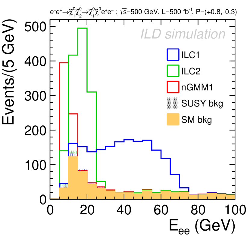
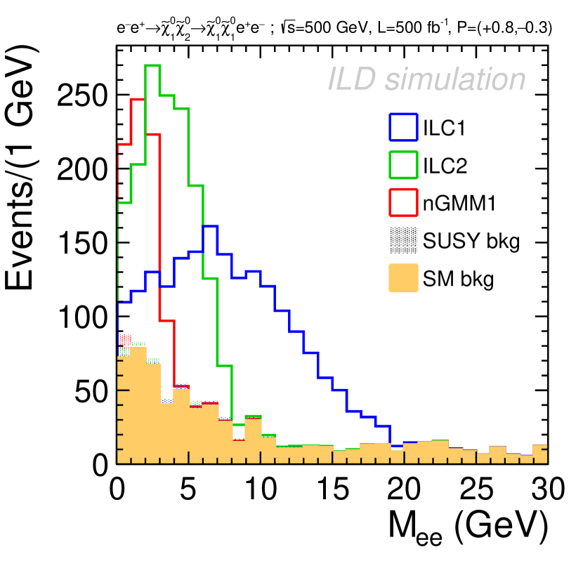
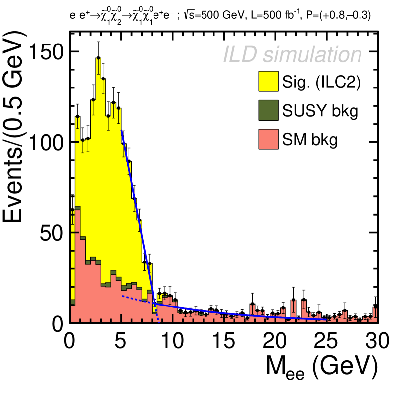
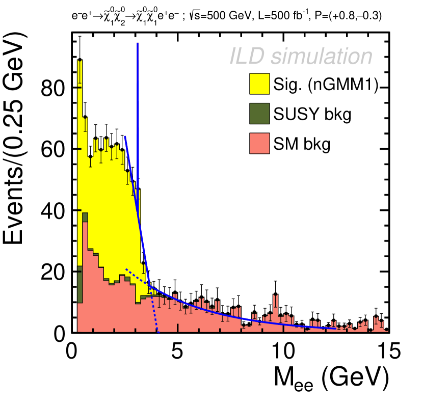
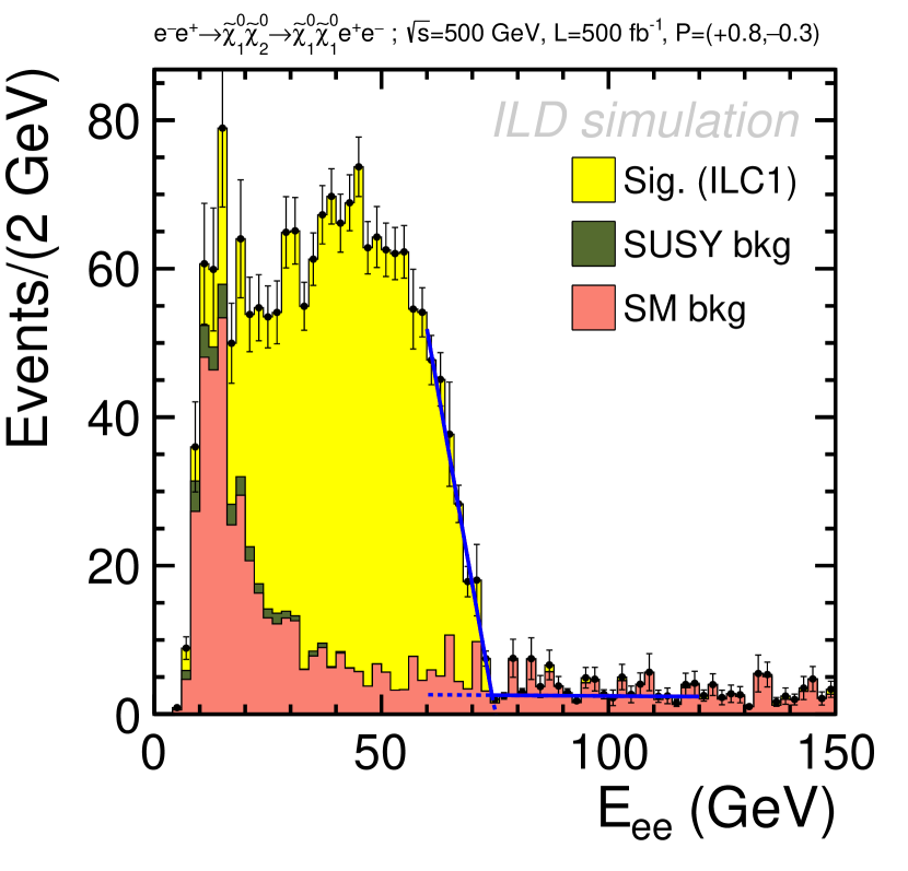
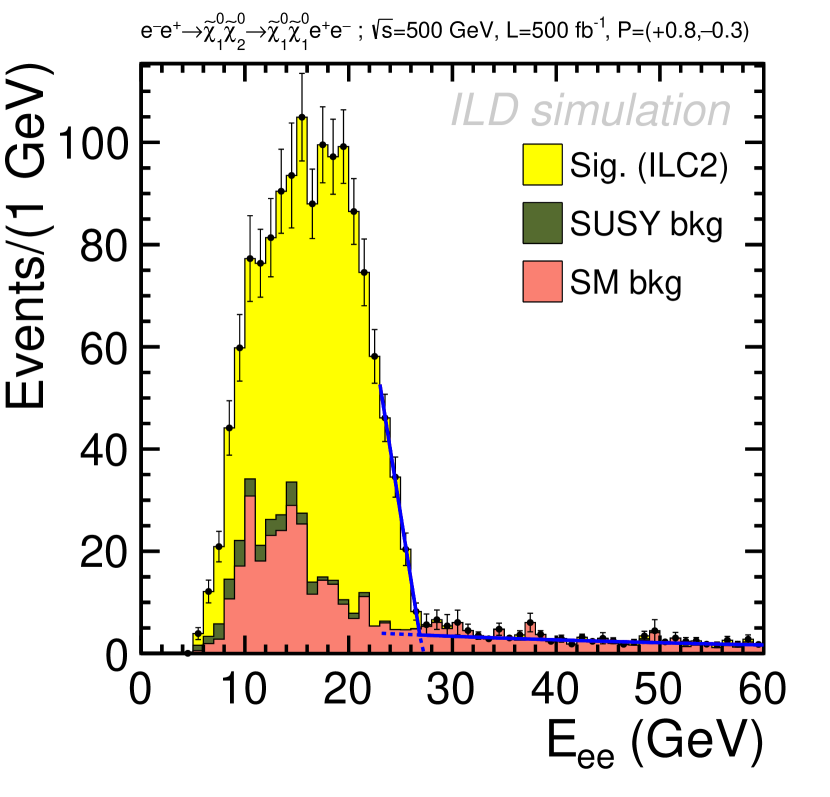
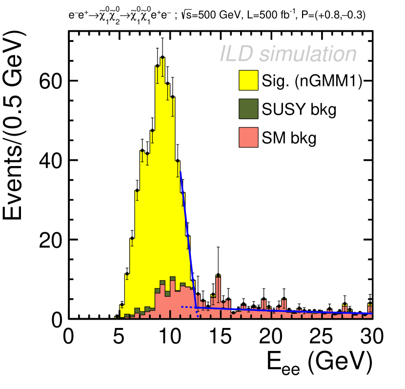
An example of the Msubscript𝑀M_{\ell\ell} and Esubscript𝐸E_{\ell\ell} distributions after this selection is shown in Fig. 8; the full distributions can be found in Appendix A. In contrast to the chargino channel, the neutralino channel has sizable SM backgrounds after the event selection, since due to the much smaller number of signal events the cuts cannot be as tight as in the chargino case. The dominant backgrounds are the e+e+νν¯superscript𝑒superscript𝑒superscriptsuperscriptsubscript𝜈superscriptsubscript¯𝜈superscripte^{+}e^{-}\rightarrow\ell^{+}\ell^{-}\nu_{\ell^{\prime}}\overline{\nu}_{\ell^{\prime}} processes, where \ell is the same lepton flavor as the final state leptons of the signal. The SUSY backgrounds remain negligible.

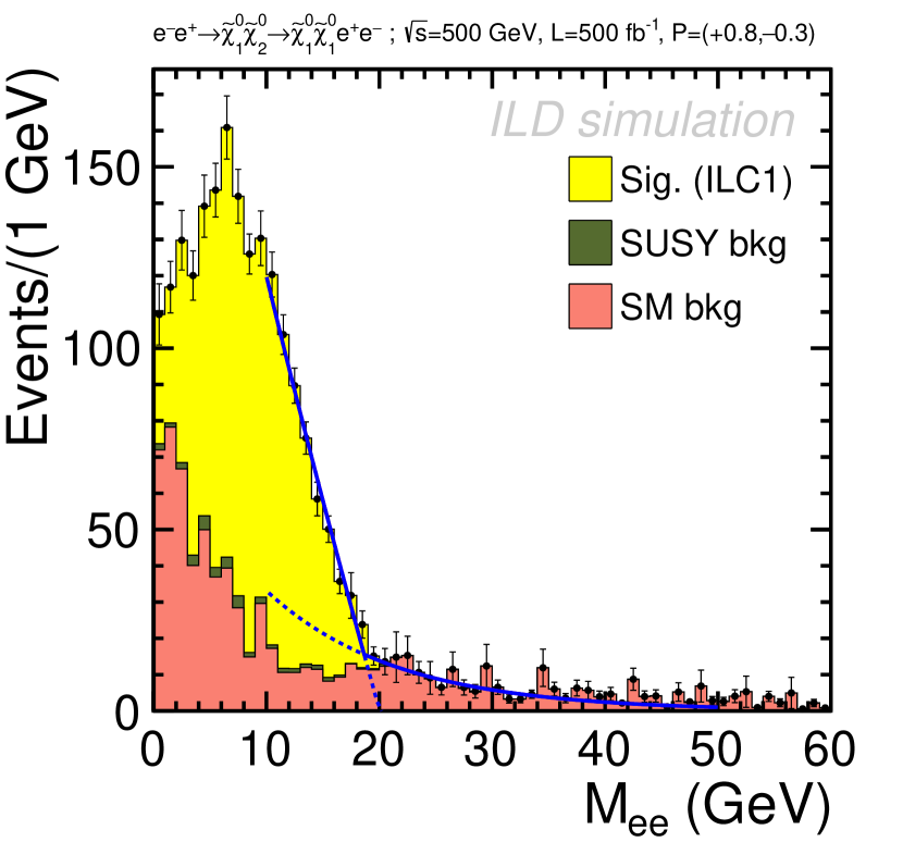
The maximum endpoints of the energy (Esubscript𝐸E_{\ell\ell}) and mass (Msubscript𝑀M_{\ell\ell}) distributions of the di-lepton system are extracted using a fit. We show some examples of the fit in Figs. 9-10. We use an exponential curve to model the background near the endpoint. A linear function is used to model the signal part. The intersection of the two functions is used to extract the kinematic endpoint. Again, the uncertainty of this value is estimated using toy Monte-Carlo experiments. Fitting the invariant mass distribution in the nGMM1 benchmark point requires special care due to the J/ψ𝐽𝜓J/\psi resonance from the neutralino decay, which sits on the falling end of the distribution. The fit is done in two steps. First, a Gaussian distribution with a narrow width is used to fit the narrow peak in the small window of the J/ψ𝐽𝜓J/\psi resonance. The fitted yield and width of the resonance are fixed in the second, overall fit, which extracts the maximum endpoint. As was the case for the chargino channel, the extracted maximum endpoint of the dilepton mass distributions requires a correction at the level of 10-20% before they are used input to the final fit for the masses, while the endpoints from the dilepton energy distributions are used without corrections.

Table 7: Expected number of events after the event selction for the neutralino signal and major backgrounds, normalized to an integrated luminosity of 500 fb-1. For each benchmark model the SUSY background is given in the column “Bkg.”.
e+eχ~10χ~20superscript𝑒superscript𝑒subscriptsuperscript~𝜒01subscriptsuperscript~𝜒02e^{+}e^{-}\rightarrow\widetilde{\chi}^{0}_{1}\widetilde{\chi}^{0}_{2} ILC1 ILC2 nGMM1 SM bkg.
Process 𝒫𝒫\mathcal{P} Sig. Bkg. Sig. Bkg. Sig. Bkg. e+esuperscript𝑒superscript𝑒absente^{+}e^{-}\rightarrow 2f e+esuperscript𝑒superscript𝑒absente^{+}e^{-}\rightarrow 4f γγ𝛾𝛾absent\gamma\gamma\rightarrow 2f eγ𝑒𝛾absente\gamma\rightarrow 3f γγ𝛾𝛾absent\gamma\gamma\rightarrow 4f
ee𝑒𝑒ee 𝒫+subscript𝒫absent\mathcal{P}_{-+} 1621 185 1250 226 490 207 14 3875 14 371 19
𝒫+subscript𝒫absent\mathcal{P}_{+-} 1284 69 1017 111 409 119 13 508 14 83 19
μμ𝜇𝜇\mu\mu 𝒫+subscript𝒫absent\mathcal{P}_{-+} 1939 176 1496 197 640 91 0.0 5506 77 100 9.6
𝒫+subscript𝒫absent\mathcal{P}_{+-} 1521 49 1222 67 516 40 0.0 672 77 100 9.6
Refer to caption
(a) di-jet energy
Refer to caption
(b) di-jet mass
Figure 8: Example of reconstructed distributions in the neutralino channel ee+χ~10χ~20χ~10χ~10e+esuperscript𝑒superscript𝑒superscriptsubscript~𝜒10superscriptsubscript~𝜒20superscriptsubscript~𝜒10superscriptsubscript~𝜒10superscript𝑒superscript𝑒e^{-}e^{+}\rightarrow\tilde{\chi}_{1}^{0}\tilde{\chi}_{2}^{0}\rightarrow\tilde{\chi}_{1}^{0}\tilde{\chi}_{1}^{0}e^{+}e^{-} with beam polarization 𝒫+subscript𝒫absent\mathcal{P}_{+-}. The signal histograms are stacked on top of the backgrounds. The remaining background is fully dominated by the SM contribution.
Refer to caption
(a) ILC1
Refer to caption
(b) ILC2
Refer to caption
(c) nGMM1
Figure 9: Example of the endpoint extraction of the di-lepton invariant mass system in the neutralino channel ee+χ~10χ~20χ~10χ~10e+esuperscript𝑒superscript𝑒superscriptsubscript~𝜒10superscriptsubscript~𝜒20superscriptsubscript~𝜒10superscriptsubscript~𝜒10superscript𝑒superscript𝑒e^{-}e^{+}\rightarrow\tilde{\chi}_{1}^{0}\tilde{\chi}_{2}^{0}\rightarrow\tilde{\chi}_{1}^{0}\tilde{\chi}_{1}^{0}e^{+}e^{-} with beam polarization 𝒫+subscript𝒫absent\mathcal{P}_{+-} for the three benchmarks. For the nGMM1 benchmark, the J/ψ𝐽𝜓J/\psi peak is included in the fit.
Refer to caption
(a) ILC1
Refer to caption
(b) ILC2
Refer to caption
(c) nGMM1
Figure 10: Example of the endpoint extraction of the di-lepton energy system in the neutralino channel ee+χ~10χ~20χ~10χ~10e+esuperscript𝑒superscript𝑒superscriptsubscript~𝜒10superscriptsubscript~𝜒20superscriptsubscript~𝜒10superscriptsubscript~𝜒10superscript𝑒superscript𝑒e^{-}e^{+}\rightarrow\tilde{\chi}_{1}^{0}\tilde{\chi}_{2}^{0}\rightarrow\tilde{\chi}_{1}^{0}\tilde{\chi}_{1}^{0}e^{+}e^{-} with beam polarization 𝒫+subscript𝒫absent\mathcal{P}_{+-} for the three benchmarks.

4.3 Results from the full detector simulation study

We present the combined result of the mass measurements in Tab. 8. Assuming an integrated luminosity of 500 fb-1 at each of the two beam polarizations P(e+superscript𝑒e^{+}, esuperscript𝑒e^{-}) = (±plus-or-minus\pm30%percent\% ,minus-or-plus\mp80%percent\%), it is shown that the chargino and neutralino masses can be measured to about 0.5-0.7%percent\% for benchmarks with mass gaps of 10 GeV or larger, and better than 1%percent\% for benchmarks with mass gaps of a few GeV.

Table 8: ILC1, ILC2 and nGMM1 MSSM model masses from Isajet (see also Tab. 1). Experimental mass precision from s=500𝑠500\sqrt{s}=500 GeV and =500500\mathcal{L}=500 fb-1 combining both beam polarizations. It is assumed that the same precision is valid for these masses as the simulation shows for the Isajet masses. The scaled precision for 1600 fb-1 for each of the two opposite-sign polarisation configurations at s=500 GeV𝑠500 GeV\sqrt{s}=500\text{ GeV}, ignoring the data sets with other centre-of-mass energies in the H20 and I20 operating scenarios.
s=500𝑠500\sqrt{s}=500 GeV only ILC1 ILC2 nGMM1
Model mass [GeV] mχ~10subscript𝑚superscriptsubscript~𝜒10m_{\widetilde{\chi}_{1}^{0}} 102.7 148.1 151.4
mχ~20subscript𝑚superscriptsubscript~𝜒20m_{\widetilde{\chi}_{2}^{0}} 124.0 157.8 155.8
mχ~1±subscript𝑚superscriptsubscript~𝜒1plus-or-minusm_{\widetilde{\chi}_{1}^{\pm}} 117.3 158.3 158.7
Precision δmχ~10/mχ~10𝛿subscript𝑚superscriptsubscript~𝜒10subscript𝑚superscriptsubscript~𝜒10\delta m_{\widetilde{\chi}_{1}^{0}}/m_{\widetilde{\chi}_{1}^{0}} 0.5 % 0.7 % 1.0 %
(𝒫+subscript𝒫absent\mathcal{P}_{-+}, =500500\mathcal{L}=500 fb-1) δmχ~20/mχ~20𝛿subscript𝑚superscriptsubscript~𝜒20subscript𝑚superscriptsubscript~𝜒20\delta m_{\widetilde{\chi}_{2}^{0}}/m_{\widetilde{\chi}_{2}^{0}} 0.5 % 0.7 % 1.0 %
direct-sum\oplus (𝒫+subscript𝒫absent\mathcal{P}_{+-}, =500500\mathcal{L}=500 fb-1) δmχ~1±/mχ~1±𝛿subscript𝑚superscriptsubscript~𝜒1plus-or-minussubscript𝑚superscriptsubscript~𝜒1plus-or-minus\delta m_{\widetilde{\chi}_{1}^{\pm}}/m_{\widetilde{\chi}_{1}^{\pm}} 0.5 % 0.7 % 1.0 %
Scaled precision δmχ~10/mχ~10𝛿subscript𝑚superscriptsubscript~𝜒10subscript𝑚superscriptsubscript~𝜒10\delta m_{\widetilde{\chi}_{1}^{0}}/m_{\widetilde{\chi}_{1}^{0}} 0.3 % 0.4 % 0.5%
(𝒫+subscript𝒫absent\mathcal{P}_{-+}, =16001600\mathcal{L}=1600 fb-1) δmχ~20/mχ~20𝛿subscript𝑚superscriptsubscript~𝜒20subscript𝑚superscriptsubscript~𝜒20\delta m_{\widetilde{\chi}_{2}^{0}}/m_{\widetilde{\chi}_{2}^{0}} 0.3 % 0.4 % 0.5%
direct-sum\oplus (𝒫+subscript𝒫absent\mathcal{P}_{+-}, =16001600\mathcal{L}=1600 fb-1) δmχ~1±/mχ~1±𝛿subscript𝑚superscriptsubscript~𝜒1plus-or-minussubscript𝑚superscriptsubscript~𝜒1plus-or-minus\delta m_{\widetilde{\chi}_{1}^{\pm}}/m_{\widetilde{\chi}_{1}^{\pm}} 0.3 % 0.4 % 0.5%

In the last column, the relative precisions on the masses have been scaled to the full luminosity foreseen to be collected at s=500𝑠500\sqrt{s}=500 GeV according to the H20 and I20 running scenarios of the ILC [68]. These values are considered to be conservative as they neglect further improvements from data sets at lower center-of-mass energies or from dedicated threshold scans. The relative precisions on the masses range from 0.3% in case of ILC1 with the largest mass differences to about 0.6% for nGMM1 as the case with the smallest mass differences.

The precision expected for the cross section times branching ratio measurements at s=500𝑠500\sqrt{s}=500 GeV is estimated from the statistical significance computed from the number of signal and background events using the di-lepton and di-jet energy distributions. In the case of the neutralino channel, an additional cut on the di-lepton mass distribution is applied in order to remove the SM backgrounds in the high mass region; namely, events with MMsubscript𝑀subscriptMM_{\mathrm{M_{\ell\ell}}} less than 25, 15, and 5 GeV are selected for the ILC1, ILC2, and nGMM1 benchmarks, respectively. The acepted region of the energy distribution is optimized to yield the best statistical significance for each channel. These were extrapolated to lower center-of-mass energies based on cross section and luminosity scaling. In most cases, the cross sections can be measured with a precision of a few %percent\%, as summarized in Tab. 9. Notorical exception are the chargino cross sections for the 𝒫+subscript𝒫absent\mathcal{P}_{+-} case, which are typically a factor two worse than the other precisions.

Table 9: Estimated experimental precisions for the three benchmark points, for the four different final states and the two beam polarizations. The full simulation results, performed for s=500𝑠500\sqrt{s}=500 GeV, are given for =500500\mathcal{L}=500 fb-1. The scaled precisions for the various center-of-mass energies are shown assuming the H20 scenario for ILC1 and the I20 scenario for ILC2 and nGMM1.
Δ(σ×BR)Δ𝜎𝐵𝑅\Delta(\sigma\times BR) [%] s=500𝑠500\sqrt{s}=500 GeV s=500𝑠500\sqrt{s}=500 GeV s=250𝑠250\sqrt{s}=250 GeV s=350𝑠350\sqrt{s}=350 GeV
𝒫+subscript𝒫absent\mathcal{P}_{-+} 𝒫+subscript𝒫absent\mathcal{P}_{+-} 𝒫+subscript𝒫absent\mathcal{P}_{-+} 𝒫+subscript𝒫absent\mathcal{P}_{+-} 𝒫+subscript𝒫absent\mathcal{P}_{-+} 𝒫+subscript𝒫absent\mathcal{P}_{+-} 𝒫+subscript𝒫absent\mathcal{P}_{-+} 𝒫+subscript𝒫absent\mathcal{P}_{+-}
ILC1 =500500\mathcal{L}=500 fb-1 Scaled (H20)
χ~10χ~20χ~10χ~10eesuperscriptsubscript~𝜒10superscriptsubscript~𝜒20superscriptsubscript~𝜒10superscriptsubscript~𝜒10𝑒𝑒\widetilde{\chi}_{1}^{0}\widetilde{\chi}_{2}^{0}\rightarrow\widetilde{\chi}_{1}^{0}\widetilde{\chi}_{1}^{0}ee 3.98 3.13 2.22 1.75 2.04 1.60 6.94 5.47
χ~10χ~20χ~10χ~10μμsuperscriptsubscript~𝜒10superscriptsubscript~𝜒20superscriptsubscript~𝜒10superscriptsubscript~𝜒10𝜇𝜇\widetilde{\chi}_{1}^{0}\widetilde{\chi}_{2}^{0}\rightarrow\widetilde{\chi}_{1}^{0}\widetilde{\chi}_{1}^{0}\mu\mu 3.81 2.97 2.13 1.66 1.95 1.52 6.66 5.18
χ~1+χ~1χ~10χ~10qqeνesubscriptsuperscript~𝜒1subscriptsuperscript~𝜒1superscriptsubscript~𝜒10superscriptsubscript~𝜒10𝑞𝑞𝑒subscript𝜈𝑒\widetilde{\chi}^{+}_{1}\widetilde{\chi}^{-}_{1}\rightarrow\widetilde{\chi}_{1}^{0}\widetilde{\chi}_{1}^{0}qqe\nu_{e} 2.59 4.94 1.45 2.76 1.61 3.22 4.66 9.04
χ~1+χ~1χ~10χ~10qqμνμsubscriptsuperscript~𝜒1subscriptsuperscript~𝜒1superscriptsubscript~𝜒10superscriptsubscript~𝜒10𝑞𝑞𝜇subscript𝜈𝜇\widetilde{\chi}^{+}_{1}\widetilde{\chi}^{-}_{1}\rightarrow\widetilde{\chi}_{1}^{0}\widetilde{\chi}_{1}^{0}qq\mu\nu_{\mu} 2.27 4.30 1.27 2.40 1.41 2.80 4.09 7.87
ILC2 =500500\mathcal{L}=500 fb-1 Scaled (I20)
χ~10χ~20χ~10χ~10eesuperscriptsubscript~𝜒10superscriptsubscript~𝜒20superscriptsubscript~𝜒10superscriptsubscript~𝜒10𝑒𝑒\widetilde{\chi}_{1}^{0}\widetilde{\chi}_{2}^{0}\rightarrow\widetilde{\chi}_{1}^{0}\widetilde{\chi}_{1}^{0}ee 3.92 3.50 2.19 1.96 - - 2.82 2.52
χ~10χ~20χ~10χ~10μμsuperscriptsubscript~𝜒10superscriptsubscript~𝜒20superscriptsubscript~𝜒10superscriptsubscript~𝜒10𝜇𝜇\widetilde{\chi}_{1}^{0}\widetilde{\chi}_{2}^{0}\rightarrow\widetilde{\chi}_{1}^{0}\widetilde{\chi}_{1}^{0}\mu\mu 3.90 3.33 2.18 1.86 - - 2.81 2.40
χ~1+χ~1χ~10χ~10qqeνesubscriptsuperscript~𝜒1subscriptsuperscript~𝜒1superscriptsubscript~𝜒10superscriptsubscript~𝜒10𝑞𝑞𝑒subscript𝜈𝑒\widetilde{\chi}^{+}_{1}\widetilde{\chi}^{-}_{1}\rightarrow\widetilde{\chi}_{1}^{0}\widetilde{\chi}_{1}^{0}qqe\nu_{e} 5.17 10.30 2.89 5.76 - - 4.09 8.28
χ~1+χ~1χ~10χ~10qqμνμsubscriptsuperscript~𝜒1subscriptsuperscript~𝜒1superscriptsubscript~𝜒10superscriptsubscript~𝜒10𝑞𝑞𝜇subscript𝜈𝜇\widetilde{\chi}^{+}_{1}\widetilde{\chi}^{-}_{1}\rightarrow\widetilde{\chi}_{1}^{0}\widetilde{\chi}_{1}^{0}qq\mu\nu_{\mu} 4.39 8.84 2.45 4.94 - - 3.47 7.10
nGMM1 =500500\mathcal{L}=500 fb-1 Scaled (I20)
χ~10χ~20χ~10χ~10eesuperscriptsubscript~𝜒10superscriptsubscript~𝜒20superscriptsubscript~𝜒10superscriptsubscript~𝜒10𝑒𝑒\widetilde{\chi}_{1}^{0}\widetilde{\chi}_{2}^{0}\rightarrow\widetilde{\chi}_{1}^{0}\widetilde{\chi}_{1}^{0}ee 5.30 4.98 2.96 2.78 - - 3.84 3.61
χ~10χ~20χ~10χ~10μμsuperscriptsubscript~𝜒10superscriptsubscript~𝜒20superscriptsubscript~𝜒10superscriptsubscript~𝜒10𝜇𝜇\widetilde{\chi}_{1}^{0}\widetilde{\chi}_{2}^{0}\rightarrow\widetilde{\chi}_{1}^{0}\widetilde{\chi}_{1}^{0}\mu\mu 5.05 4.64 2.82 2.59 - - 3.66 3.36
χ~1+χ~1χ~10χ~10qqeνesubscriptsuperscript~𝜒1subscriptsuperscript~𝜒1superscriptsubscript~𝜒10superscriptsubscript~𝜒10𝑞𝑞𝑒subscript𝜈𝑒\widetilde{\chi}^{+}_{1}\widetilde{\chi}^{-}_{1}\rightarrow\widetilde{\chi}_{1}^{0}\widetilde{\chi}_{1}^{0}qqe\nu_{e} 6.20 11.73 3.47 6.56 - - 4.94 9.48
χ~1+χ~1χ~10χ~10qqμνμsubscriptsuperscript~𝜒1subscriptsuperscript~𝜒1superscriptsubscript~𝜒10superscriptsubscript~𝜒10𝑞𝑞𝜇subscript𝜈𝜇\widetilde{\chi}^{+}_{1}\widetilde{\chi}^{-}_{1}\rightarrow\widetilde{\chi}_{1}^{0}\widetilde{\chi}_{1}^{0}qq\mu\nu_{\mu} 4.99 9.90 2.79 5.53 - - 3.98 8.00

5 Fitting fundamental parameters

In this section we will pursue the question of whether the projected precisions on the physics observables will be sufficient to discriminate between different SUSY models, and to determine the parameters of the correct model. To this purpose, assumed measurements of Higgsino masses and polarized cross sections are presented to Fittino along with their projected uncertainties. It should be noted that the asummed measurements have not been varied randomly around their true values. Thus, in all cases where the correct underlying model is fitted, the expected χ2superscript𝜒2\chi^{2} is zero, apart from effects of finite numerical precision and the finite length of the Markov chains. As discussed in Sec. 3.4, SPheno had to be used instead of Isajet as a spectrum calculator in the fitting step.666Here we switch to the spectrum generator SPheno since there exists a direct interface between SPeno and Fittino while no such interface exists for Fittino and Isajet. The mass spectra generated from Isajet and SPheno are slightly different due to different algorithms used by the code authors.

The fits include the following inputs based on ILC simulation studies:

  • The higgsino masses obtained with SPheno3.3.9beta as listed in Tab. 10, together with their estimated precisions based on a preliminary version of the full simulation study at s=500𝑠500\sqrt{s}=500 GeV, listed in Tab. 7.11 of Ref. [66]. Note that these are between 30% and 100% more conservative than the results given in Tab. 8 of this paper. We will study and discuss the relevance of these differences in Sec. 6.4.

  • The polarised total cross sections for chargino and neutralino production at all relevant center-of-mass energies with precisions as given in Tab. 7.12-7.14 of Ref. [66]. As for the masses, these are between 20% and 100% more conservative than the full simulation results listed in Tab. 9, and we will study and discuss the relevance of these differences in Sec. 6.4. Note that in ILC1, higgsino production is kinematically accessible at center-of-mass energies as low as 250250250 GeV, while for ILC2 and nGMM1 s=350𝑠350\sqrt{s}=350 GeV is the lowest ILC energy stage which allows higgsino production. Therefore, we consider the alternative running scenario I20 [68] for these benchmarks.

  • The mass of the lightest CP𝐶𝑃CP-even Higgs boson, with the ILC precision according to [69], as discussed in Sec. 3.4.

  • The branching ratios BR(hbb¯)𝐵𝑅𝑏¯𝑏BR(h\rightarrow b\bar{b}), BR(hcc¯)𝐵𝑅𝑐¯𝑐BR(h\rightarrow c\bar{c}), BR(hτ+τ)𝐵𝑅superscript𝜏superscript𝜏BR(h\rightarrow\tau^{+}\tau^{-}), BR(hgg)𝐵𝑅𝑔𝑔BR(h\rightarrow gg), BR(hW+W)𝐵𝑅superscript𝑊superscript𝑊BR(h\rightarrow W^{+}W^{-}), BR(hZZ)𝐵𝑅𝑍𝑍BR(h\rightarrow ZZ) and BR(hγγ)𝐵𝑅𝛾𝛾BR(h\rightarrow\gamma\gamma), with the ILC precisions according to [68], as discussed in Sec. 3.4.

In total, these amount to 25 observables. In the following, we will start by discussing fits of different GUT-scale models in Sec. 5.1, and before proceeding to the determination of weak-scale parameters in Sec. 5.2. Finally, we will address the predictions of the LSP’s relic density in Sec. 5.3.

Table 10: ILC1, ILC2 and nGMM1 MSSM model masses from SPheno3.3.9beta together with the input precisions assumed in the fit. The assumed input precisions are given for s=500𝑠500\sqrt{s}=500 GeV and =16001600\mathcal{L}=1600 fb-1. Data sets with other center-of-mass energies in the H20 and I20 operating scenarios are neglected.
s=500𝑠500\sqrt{s}=500 GeV only ILC1 ILC2 nGMM1
Model mass [GeV] mχ~10subscript𝑚superscriptsubscript~𝜒10m_{\widetilde{\chi}_{1}^{0}} 104.8 151.3 154.9
mχ~20subscript𝑚superscriptsubscript~𝜒20m_{\widetilde{\chi}_{2}^{0}} 127.5 162.4 160.2
mχ~1±subscript𝑚superscriptsubscript~𝜒1plus-or-minusm_{\widetilde{\chi}_{1}^{\pm}} 116.0 157.0 157.4
Assumed precision δmχ~10/mχ~10𝛿subscript𝑚superscriptsubscript~𝜒10subscript𝑚superscriptsubscript~𝜒10\delta m_{\widetilde{\chi}_{1}^{0}}/m_{\widetilde{\chi}_{1}^{0}} 0.5% 0.7% 1.0%
(𝒫+subscript𝒫absent\mathcal{P}_{-+}, =16001600\mathcal{L}=1600 fb-1) δmχ~20/mχ~20𝛿subscript𝑚superscriptsubscript~𝜒20subscript𝑚superscriptsubscript~𝜒20\delta m_{\widetilde{\chi}_{2}^{0}}/m_{\widetilde{\chi}_{2}^{0}} 0.4% 0.7% 1.0%
direct-sum\oplus (𝒫+subscript𝒫absent\mathcal{P}_{+-}, =16001600\mathcal{L}=1600 fb-1) δmχ~1±/mχ~1±𝛿subscript𝑚superscriptsubscript~𝜒1plus-or-minussubscript𝑚superscriptsubscript~𝜒1plus-or-minus\delta m_{\widetilde{\chi}_{1}^{\pm}}/m_{\widetilde{\chi}_{1}^{\pm}} 0.5% 0.7% 1.0%

5.1 Fitting GUT-scale parameters

The fitting of GUT-scale parameters requires strong assumptions on the underlying SUSY breaking scheme. Since our benchmarks cover two very different approaches to unification, it is interesting to study whether these can be distinguished by directly fitting different GUT-scale models.

5.1.1 Results of fitting NUHM2

In case of NUHM2, we fit the parameters M1/2subscript𝑀12M_{1/2}, μ𝜇\mu, tanβ𝛽\tan\beta, M0subscript𝑀0M_{0}, A0subscript𝐴0A_{0} and mAsubscript𝑚𝐴m_{A} to the observables described in Sec. 4.3. Table 11 shows the best fit point and its 1 and 2σ𝜎\sigma confidence intervals obtained in the case of the ILC1 benchmark, in comparison to the input model parameters. Tables 12 and 13 give the analogous information for the ILC2 and nGMM1 benchmarks, respectively. In case of the ILC1 and ILC2 benchmarks, where NUHM2 is the correct underlying model, the χ2superscript𝜒2\chi^{2} of the best fit point is very small, and all fitted parameters agree well with their true input values. The 1σ𝜎\sigma uncertainties for M1/2subscript𝑀12M_{1/2}, μ𝜇\mu, tanβ𝛽\tan\beta are typically 10% or better, while M0subscript𝑀0M_{0}, A0subscript𝐴0A_{0} and mAsubscript𝑚𝐴m_{A}, which enter only at loop-level into the considered observables, are still determined within about 20%.

parameterILC1 NUHM2 truebest fit point 1σ CL2σ CLM1/2568.3556.720.3+24.343.1+37.7μ115.0105.38.2+12.814.5+14.0tanβ10.011.41.6+5.61.6+11.4mA100096865+167130+288M0702576851917+12432095+2311A010427110641422+26952698+2927χ20.00130.0011missing-subexpressionmissing-subexpressionmissing-subexpressionmissing-subexpressionmissing-subexpressionmissing-subexpressionmissing-subexpressionmissing-subexpressionmissing-subexpressionmissing-subexpressionmissing-subexpressionmissing-subexpressionmissing-subexpressionmissing-subexpressionparameterILC1 NUHM2 truebest fit point 1𝜎 CL2𝜎 CLmissing-subexpressionmissing-subexpressionmissing-subexpressionmissing-subexpressionmissing-subexpressionmissing-subexpressionmissing-subexpressionmissing-subexpressionmissing-subexpressionsubscript𝑀12568.3556.7subscriptsuperscriptabsent24.320.3subscriptsuperscriptabsent37.743.1missing-subexpressionmissing-subexpression𝜇115.0105.3subscriptsuperscriptabsent12.88.2subscriptsuperscriptabsent14.014.5missing-subexpressionmissing-subexpression𝛽10.011.4subscriptsuperscriptabsent5.61.6subscriptsuperscriptabsent11.41.6missing-subexpressionmissing-subexpressionsubscript𝑚𝐴1000968subscriptsuperscriptabsent16765subscriptsuperscriptabsent288130missing-subexpressionmissing-subexpressionsubscript𝑀070257685subscriptsuperscriptabsent12431917subscriptsuperscriptabsent23112095missing-subexpressionmissing-subexpressionsubscript𝐴01042711064subscriptsuperscriptabsent26951422subscriptsuperscriptabsent29272698missing-subexpressionmissing-subexpressionmissing-subexpressionmissing-subexpressionmissing-subexpressionmissing-subexpressionmissing-subexpressionmissing-subexpressionmissing-subexpressionsuperscript𝜒20.00130.0011missing-subexpressionmissing-subexpressionmissing-subexpressionmissing-subexpressionmissing-subexpressionmissing-subexpressionmissing-subexpressionmissing-subexpressionmissing-subexpressionmissing-subexpressionmissing-subexpression\begin{array}[]{ c c c c c c c }\hline\cr\hline\cr\text{parameter}&\text{ILC1 NUHM2 true}&\text{best fit point }&1\sigma\text{ CL}&2\sigma\text{ CL}\\ \hline\cr M_{1/2}&568.3&556.7&\ {}^{+24.3}_{-20.3}&\ {}^{+37.7}_{-43.1}\\ \mu&115.0&105.3&\ {}^{+12.8}_{-8.2}&\ {}^{+14.0}_{-14.5}\\ \tan\beta&10.0&11.4&\ {}^{+5.6}_{-1.6}&\ {}^{+11.4}_{-1.6}\\ m_{A}&1000&968&\ {}^{+167}_{-65}&\ {}^{+288}_{-130}\\ M_{0}&7025&7685&\ {}^{+1243}_{-1917}&\ {}^{+2311}_{-2095}\\ A_{0}&-10427&-11064&\ {}^{+2695}_{-1422}&\ {}^{+2927}_{-2698}\\ \hline\cr\chi^{2}&0.0013&0.0011&&\\ \hline\cr\hline\cr\end{array}

Table 11: Fitted parameters in the fit of NUHM2 parameters to ILC1 observables in the H20 scenario. All values in GeV apart from tanβ𝛽\tan{\beta}. Note that the χ2superscript𝜒2\chi^{2} value of the model point is increased from 0 by the rounding errors of the observables in the inputs.

parameterILC2 NUHM2 truebest fit point 1σ CL2σ CLM1/21200119468+107129+164μ150.0150.74.5+4.35.2+7.2tanβ15.016.06.6+26.26.6+28.8mA10001008118+141196+256M0500047883137+25463283+3566A0800076633926+38175342+3817χ20.00070.02848missing-subexpressionmissing-subexpressionmissing-subexpressionmissing-subexpressionmissing-subexpressionmissing-subexpressionmissing-subexpressionmissing-subexpressionmissing-subexpressionmissing-subexpressionmissing-subexpressionmissing-subexpressionmissing-subexpressionmissing-subexpressionparameterILC2 NUHM2 truebest fit point 1𝜎 CL2𝜎 CLmissing-subexpressionmissing-subexpressionmissing-subexpressionmissing-subexpressionmissing-subexpressionmissing-subexpressionmissing-subexpressionmissing-subexpressionmissing-subexpressionsubscript𝑀1212001194subscriptsuperscriptabsent10768subscriptsuperscriptabsent164129missing-subexpressionmissing-subexpression𝜇150.0150.7subscriptsuperscriptabsent4.34.5subscriptsuperscriptabsent7.25.2missing-subexpressionmissing-subexpression𝛽15.016.0subscriptsuperscriptabsent26.26.6subscriptsuperscriptabsent28.86.6missing-subexpressionmissing-subexpressionsubscript𝑚𝐴10001008subscriptsuperscriptabsent141118subscriptsuperscriptabsent256196missing-subexpressionmissing-subexpressionsubscript𝑀050004788subscriptsuperscriptabsent25463137subscriptsuperscriptabsent35663283missing-subexpressionmissing-subexpressionsubscript𝐴080007663subscriptsuperscriptabsent38173926subscriptsuperscriptabsent38175342missing-subexpressionmissing-subexpressionmissing-subexpressionmissing-subexpressionmissing-subexpressionmissing-subexpressionmissing-subexpressionmissing-subexpressionmissing-subexpressionsuperscript𝜒20.00070.02848missing-subexpressionmissing-subexpressionmissing-subexpressionmissing-subexpressionmissing-subexpressionmissing-subexpressionmissing-subexpressionmissing-subexpressionmissing-subexpressionmissing-subexpressionmissing-subexpression\begin{array}[]{ c c c c c c c }\hline\cr\hline\cr\text{parameter}&\text{ILC2 NUHM2 true}&\text{best fit point }&1\sigma\text{ CL}&2\sigma\text{ CL}\\ \hline\cr M_{1/2}&1200&1194&\ {}^{+107}_{-68}&\ {}^{+164}_{-129}\\ \mu&150.0&150.7&\ {}^{+4.3}_{-4.5}&\ {}^{+7.2}_{-5.2}\\ \tan\beta&15.0&16.0&\ {}^{+26.2}_{-6.6}&\ {}^{+28.8}_{-6.6}\\ m_{A}&1000&1008&\ {}^{+141}_{-118}&\ {}^{+256}_{-196}\\ M_{0}&5000&4788&\ {}^{+2546}_{-3137}&\ {}^{+3566}_{-3283}\\ A_{0}&-8000&-7663&\ {}^{+3817}_{-3926}&\ {}^{+3817}_{-5342}\\ \hline\cr\chi^{2}&0.0007&0.02848&&\\ \hline\cr\hline\cr\end{array}

Table 12: Best fit point and confidence intervals of the NUHM2 parameters fitted to ILC2 SUSY and Higgs measurements in the I20 operating scenario. Note that the χ2superscript𝜒2\chi^{2} value of the model point is increased from 0 by the rounding errors of the observables in the inputs.

In case of the nGMM1 benchmark, the χ2superscript𝜒2\chi^{2} of the best fit point is somewhat larger than for the other two benchmarks, but still so small that an NUHM2 interpretation of this benchmark cannot be rejected. This is not surprising as it has been constructed to have the physical observables very similar to ILC2. However, the best fit point is found for M1/2subscript𝑀12M_{1/2} about a factor two bigger, and MAsubscript𝑀𝐴M_{A} about 60% larger, than in ILC2. This implies that a direct observation of the heavy Higgs bosons and the electroweakinos could distinguish the two models. However this also raises the question of whether the weak-scale fits based on input from the higgsino properties alone will be able to identify the nGMM1 benchmark unambiguously as a non-NUHM2 model, with a completely different underlying SUSY breaking mechanism. We will investigate this in the next section.
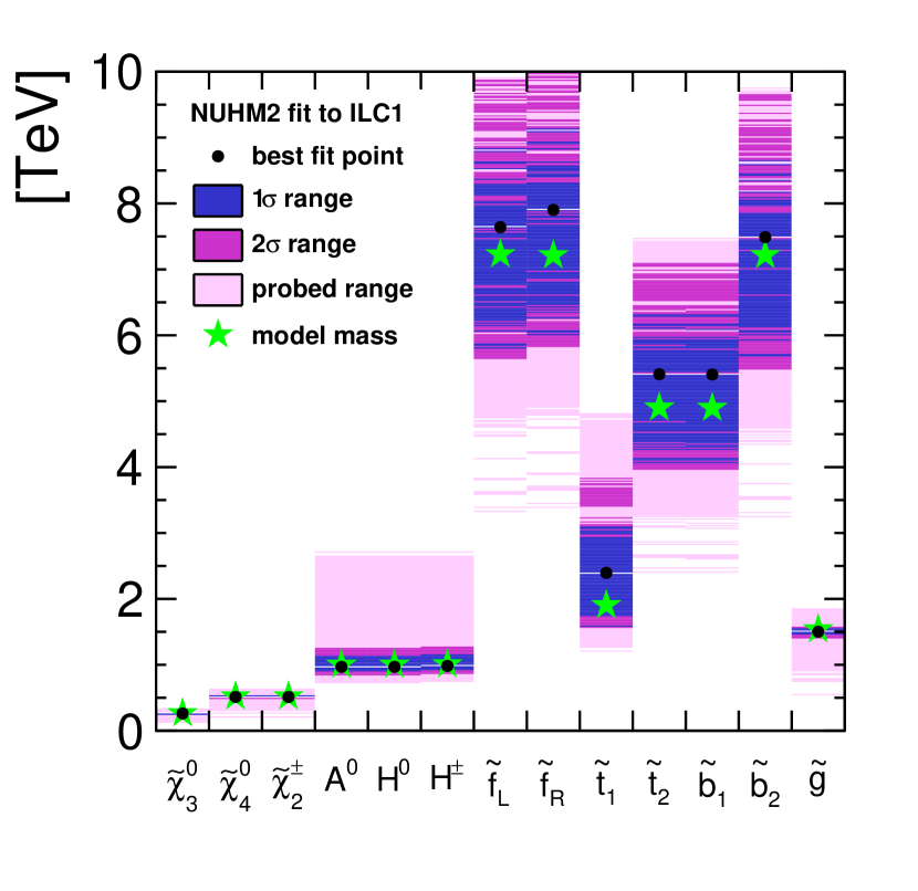
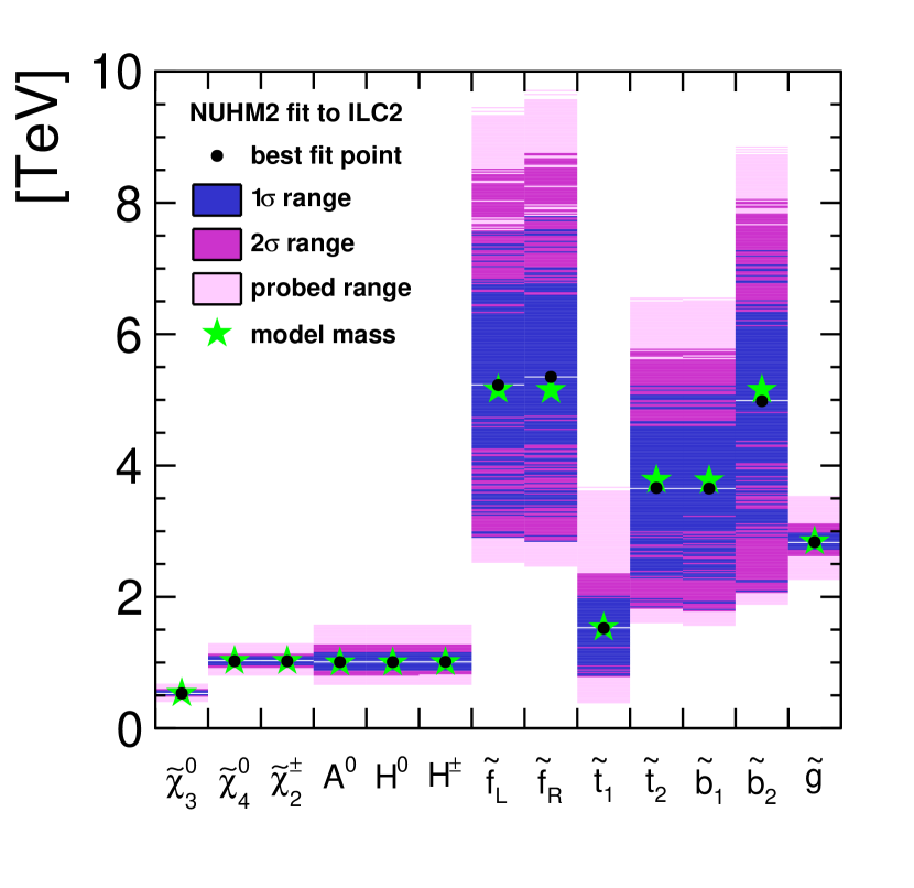
parameterbest fit point 1σ CL2σ CLM1/22407135+150215+356μ155.61.9+1.52.9+4.0tanβ10.00.5+2.10.7+2.4mA1603279+528469+1026M03422820+33091196+4435A074093756+6665304+887χ20.233missing-subexpressionmissing-subexpressionmissing-subexpressionmissing-subexpressionmissing-subexpressionmissing-subexpressionmissing-subexpressionmissing-subexpressionmissing-subexpressionmissing-subexpressionmissing-subexpressionmissing-subexpressionparameterbest fit point 1𝜎 CL2𝜎 CLmissing-subexpressionmissing-subexpressionmissing-subexpressionmissing-subexpressionmissing-subexpressionmissing-subexpressionmissing-subexpressionmissing-subexpressionsubscript𝑀122407subscriptsuperscriptabsent150135subscriptsuperscriptabsent356215missing-subexpressionmissing-subexpression𝜇155.6subscriptsuperscriptabsent1.51.9subscriptsuperscriptabsent4.02.9missing-subexpressionmissing-subexpression𝛽10.0subscriptsuperscriptabsent2.10.5subscriptsuperscriptabsent2.40.7missing-subexpressionmissing-subexpressionsubscript𝑚𝐴1603subscriptsuperscriptabsent528279subscriptsuperscriptabsent1026469missing-subexpressionmissing-subexpressionsubscript𝑀03422subscriptsuperscriptabsent3309820subscriptsuperscriptabsent44351196missing-subexpressionmissing-subexpressionsubscript𝐴07409subscriptsuperscriptabsent6663756subscriptsuperscriptabsent8875304missing-subexpressionmissing-subexpressionmissing-subexpressionmissing-subexpressionmissing-subexpressionmissing-subexpressionmissing-subexpressionmissing-subexpressionsuperscript𝜒20.233missing-subexpressionmissing-subexpressionmissing-subexpressionmissing-subexpressionmissing-subexpressionmissing-subexpressionmissing-subexpressionmissing-subexpressionmissing-subexpressionmissing-subexpression\begin{array}[]{ c c c c c c }\hline\cr\hline\cr\text{parameter}&\text{best fit point }&1\sigma\text{ CL}&2\sigma\text{ CL}\\ \hline\cr M_{1/2}&2407&\ {}^{+150}_{-135}&\ {}^{+356}_{-215}\\ \mu&155.6&\ {}^{+1.5}_{-1.9}&\ {}^{+4.0}_{-2.9}\\ \tan\beta&10.0&\ {}^{+2.1}_{-0.5}&\ {}^{+2.4}_{-0.7}\\ m_{A}&1603&\ {}^{+528}_{-279}&\ {}^{+1026}_{-469}\\ M_{0}&3422&\ {}^{+3309}_{-820}&\ {}^{+4435}_{-1196}\\ A_{0}&-7409&\ {}^{+666}_{-3756}&\ {}^{+887}_{-5304}\\ \hline\cr\chi^{2}&0.233&&\\ \hline\cr\hline\cr\end{array}

Table 13: Best fit point and confidence intervals of the NUHM2 parameters fitted to nGMM1 SUSY and Higgs measurements in the I20 operating scenario.
Refer to caption
(a) ILC1
Refer to caption
(b) ILC2
Refer to caption
(c) nGMM1
Figure 11: Predicted mass ranges for all the unobserved sparticles from the NUHM2 fit the observables of the three benchmark models. The green star indicates the true model mass, while the black dot shows the best fit point.

Based on the fitted NUHM2 parameters and their uncertainties, the mass spectrum of the unobserved sparticles can be predicted for all three benchmark cases. This is illustrated in Fig. 11. In the cases of ILC1 and ILC2, clear predictions for the masses of the electroweakinos and the heavy Higgs bosons are obtained in excellent agreement with the true model masses, providing motivation and an energy scale for further upgrades of the ILC. Due to the modelling of all gauginos by a single M1/2subscript𝑀12M_{1/2} parameter, the gluino mass can also be firmly predicted, which can give important inputs to LHC analyses. If the predicted gluino were not observed, or observed at a very different mass, this would give strong support to the idea that nature does not describe all gauginos by one mass parameter at the GUT scale. The other sfermions are less well constrained than the Higgs bosons and gauginos, but upper limits on their masses can still be obtained. Such information would provide important motivation — and a target energy scale — for a future hadron collider.

Even in case of the nGMM1 benchmark, the NUHM2 fit predicts the general pattern of the mass spectrum correctly, albeit with less precision and significantly worse agreement between true model masses and the best fit point. The worse agreement is not surprising as we’re fitting a wrong model hypothesis in this case. Nonetheless, upper limits on all sparticle masses are obtained, which shows that even in the case that the wrong model is assumed such important information for the planning of future colliders or upgrades can be obtained.

5.1.2 Results of fitting NUHM1 and CMSSM

Before turning to the weak-scale fits, we investigate whether the three benchmarks could also be described by other widely used constrained models, in particular NUHM1 [65] and the CMSSM, which have one or even two fewer parameters to model the Higgs and higgsino sectors: in NUHM1, instead of MAsubscript𝑀𝐴M_{A} and μ𝜇\mu (or MHu0subscriptsuperscript𝑀0subscript𝐻𝑢M^{0}_{H_{u}} and MHd0subscriptsuperscript𝑀0subscript𝐻𝑑M^{0}_{H_{d}}) only one parameter, MH0subscriptsuperscript𝑀0𝐻M^{0}_{H}, is used to describe the Higgs and higgsino sectors, while in the CMSSM this reduces further to only the sign of μ𝜇\mu being a free choice, while its absolute value is derived from the other model parameters. Table 14 gives the best fit point obtained when fitting NUHM1 and CMSSM to the ILC1 and ILC2 benchmarks, which give very large values of χ2/dofsuperscript𝜒2dof\chi^{2}/\textrm{dof}. These interpretations could be ruled out at the 95%percent9595\% C.L. already with about 0.1%percent0.10.1\% the total integrated luminosity.

best fit pointsparameterILC1 CMSSMILC2 CMSSMILC1 NUHM1ILC2 NUHM1M1/2[ GeV]128.8155.9136.9159.9M0[ GeV]3585563117964264A0[ GeV]687310873439610086tanβ13.716.216.214.8MH00[ GeV]4765956553χmin22380469315523501485174χ2/dof113364436117514259missing-subexpressionmissing-subexpressionmissing-subexpressionmissing-subexpressionmissing-subexpressionmissing-subexpressionmissing-subexpressionmissing-subexpressionmissing-subexpressionmissing-subexpressionbest fit pointsmissing-subexpressionmissing-subexpressionmissing-subexpressionmissing-subexpressionparameterILC1 CMSSMILC2 CMSSMILC1 NUHM1ILC2 NUHM1missing-subexpressionmissing-subexpressionmissing-subexpressionmissing-subexpressionmissing-subexpressionsubscript𝑀12delimited-[] GeV128.8155.9136.9159.9subscript𝑀0delimited-[] GeV3585563117964264subscript𝐴0delimited-[] GeV687310873439610086𝛽13.716.216.214.8subscriptsuperscript𝑀0subscript𝐻0delimited-[] GeV4765956553missing-subexpressionmissing-subexpressionmissing-subexpressionmissing-subexpressionmissing-subexpressionsubscriptsuperscript𝜒2min2380469315523501485174superscript𝜒2dof113364436117514259missing-subexpressionmissing-subexpressionmissing-subexpressionmissing-subexpressionmissing-subexpression\begin{array}[]{ c c c c c }\hline\cr\hline\cr\text{best fit points}\\ \text{parameter}&\text{ILC1 CMSSM}&\text{ILC2 CMSSM}&\text{ILC1 NUHM1}&\text{ILC2 NUHM1}\\ \hline\cr M_{1/2}[\text{ GeV}]&128.8&155.9&136.9&159.9\\ M_{0}[\text{ GeV}]&3585&5631&1796&4264\\ A_{0}[\text{ GeV}]&-6873&-10873&-4396&-10086\\ \tan\beta&13.7&16.2&16.2&14.8\\ M^{0}_{H_{0}}[\text{ GeV}]&-&-&47659&56553\\ \hline\cr\chi^{2}_{\textrm{min}}&238046&93155&235014&85174\\ \chi^{2}/\textrm{dof}&11336&4436&11751&4259\\ \hline\cr\hline\cr\end{array}

Table 14: Best fit points in CMSSM and NUHM1 fits of ILC1 and ILC2 observables, including SUSY and Higgs measurements in the H20 operation for ILC1 and I20 operation for ILC2.

5.2 Weak scale fit results

In the following, the results of various weak scale fits to the ILC1, ILC2 and nGMM1 observables are discussed. The most general model considered is pMSSM-10, the MSSM with 10 weak scale input parameters: M1subscript𝑀1M_{1}, M2subscript𝑀2M_{2}, M3subscript𝑀3M_{3}, μ𝜇\mu, tanβ𝛽\tan\beta, mAsubscript𝑚𝐴m_{A}, At=Ab=Aτsubscript𝐴𝑡subscript𝐴𝑏subscript𝐴𝜏A_{t}=A_{b}=A_{\tau} and MQ3subscript𝑀subscript𝑄3M_{Q_{3}}, MU3=MD3subscript𝑀subscript𝑈3subscript𝑀subscript𝐷3M_{U_{3}}=M_{D_{3}}, ML=ML1,2,3=ME1,2,3=MQ1,2=MU1,2=MD1,2subscript𝑀𝐿subscript𝑀subscript𝐿123subscript𝑀subscript𝐸123subscript𝑀subscript𝑄12subscript𝑀subscript𝑈12subscript𝑀subscript𝐷12M_{L}=M_{L_{1,2,3}}=M_{E_{1,2,3}}=M_{Q_{1,2}}=M_{U_{1,2}}=M_{D_{1,2}}. We use this model to test whether it is possible to constrain a comprehensive set of parameters from the observables of the higgsino sector alone, and to study the influence of the parameters in which the higgsino sector enters only at loop level. If the pMSSM-10 fit is successful and reproduces the input parameters at a satisfactory level, we proceed to investigate the precision achievable when fitting only tree-level higgsino parameters. For this we use the phenomenological MSSM with a reduced number of 4 free parameters, the pMSSM-4, which fixes the squark, slepton, heavy Higgs boson and gluino parameters to their true values and so only depends on the four weak scale parameters M1,2subscript𝑀12M_{1,2}, μ𝜇\mu and tanβ𝛽\tan\beta. In a real analysis, the “true” values are of course unknown, but instead the best fit point of pMSSM-10 fit could be used, which agrees with the model point to usually much better than 1σ𝜎\sigma. The possible bias from fixing the 6 non-higgsino parameters was tested explicitly in case of ILC1 by fixing them to some point in the 2σ𝜎\sigma region. The best fit gaugino masses are nearly the same in the two pMSSM-4 fits irrespective of the fixed parameters. Their difference is only 2.5 GeV for χ~30superscriptsubscript~𝜒30\widetilde{\chi}_{3}^{0} and 0.8 GeV for χ~40superscriptsubscript~𝜒40\widetilde{\chi}_{4}^{0} and χ~2±superscriptsubscript~𝜒2plus-or-minus\widetilde{\chi}_{2}^{\pm}. The two sets of best fit masses agree within the 1σ𝜎\sigma uncertainties [66]. In the following, the results for the individual benchmarks will be presented.

5.2.1 ILC1 Benchmark

Figure 12 shows the minimum χ2superscript𝜒2\chi^{2} as a function of M1subscript𝑀1M_{1}, M2subscript𝑀2M_{2} and μ𝜇\mu and tanβ𝛽\tan\beta in the pMSSM-10 and pMSSM-4 fits. Due to the much smaller parameter space to be sampled in case of the 4-dimensional fit, the resulting curve is much smoother than in the 10-dimensional case. The precision on M1subscript𝑀1M_{1} is nearly identical in both cases. M2subscript𝑀2M_{2} is somewhat better constrained in the pMSSM-4 fit, while the determination of μ𝜇\mu and tanβ𝛽\tan{\beta} improves drastically.

Refer to caption
(a)
Refer to caption
(b)
Refer to caption
(c)
Refer to caption
(d)
Figure 12: ILC1: Minimum χ2superscript𝜒2\chi^{2} as a function of M1subscript𝑀1M_{1}, M2subscript𝑀2M_{2} and μ𝜇\mu and tanβ𝛽\tan\beta in pMSSM-4 fit (dashed black line) and pMSSM-10 fit (solid grey line). For each bin, the minimum χ2superscript𝜒2\chi^{2} of all Markov chain points which have the x𝑥x axis quantity in that bin is plotted.

The resulting best fit values for the pMSSM parameters and their 1 and 2σ𝜎\sigma intervals are compared to the input values in Tab. 15, quantifying the effect which could already be seen qualitatively in Fig. 12. In the case of the pMSSM-10 fit, it should be noted that also for the parameters of the coloured sector some constraints, and especially upper bounds, can be obtained. This even applies for the squark mass parameters, which might seem surprising at the first glance, but is due to the 2-loop RGEs included in SPheno. If a hypothetical gluino mass measurement with 11%percent1111\% uncertainty from the LHC[Baer:2016wkz] is included in the fit, the constraint on M3subscript𝑀3M_{3} improves accordingly to about 10%percent1010\%. All other parameters, including the squark mass parameters, show only minor improvements.

pMSSM-4pMSSM-10parameterILC1 pMSSM truebest fit point1σ CL2σ CLbest fit point1σ CL2σ CLM1250250.27.7+8.215.1+17.1251.315.7+8.623.7+17.2M2463463.38.1+8.014.9+16.2465.823.0+24.249.8+31.4μ115.0115.00.2+0.20.3+0.3115.74.7+10.96.1+20.3tanβ10.010.00.1+0.10.2+0.29.73.0+8.83.5+45.3mA10001050180+310296+607M3127014121104+17912843+1411ML715070634311+20295632+2645MU(3)16701751628+2414740+4498MQ(3)482049513226+23243226+3858At=b=τ44004591973+13712949+1647χ20.00110.1360missing-subexpressionmissing-subexpressionmissing-subexpressionmissing-subexpressionmissing-subexpressionmissing-subexpressionmissing-subexpressionmissing-subexpressionmissing-subexpressionmissing-subexpressionpMSSM-4missing-subexpressionmissing-subexpressionpMSSM-10missing-subexpressionmissing-subexpressionparameterILC1 pMSSM truebest fit point1𝜎 CL2𝜎 CLbest fit point1𝜎 CL2𝜎 CLmissing-subexpressionmissing-subexpressionmissing-subexpressionmissing-subexpressionmissing-subexpressionmissing-subexpressionmissing-subexpressionmissing-subexpressionmissing-subexpressionmissing-subexpressionmissing-subexpressionmissing-subexpressionmissing-subexpressionmissing-subexpressionmissing-subexpressionmissing-subexpressionsubscript𝑀1250250.2subscriptsuperscriptabsent8.27.7subscriptsuperscriptabsent17.115.1251.3subscriptsuperscriptabsent8.615.7subscriptsuperscriptabsent17.223.7subscript𝑀2463463.3subscriptsuperscriptabsent8.08.1subscriptsuperscriptabsent16.214.9465.8subscriptsuperscriptabsent24.223.0subscriptsuperscriptabsent31.449.8𝜇115.0115.0subscriptsuperscriptabsent0.20.2subscriptsuperscriptabsent0.30.3115.7subscriptsuperscriptabsent10.94.7subscriptsuperscriptabsent20.36.1𝛽10.010.0subscriptsuperscriptabsent0.10.1subscriptsuperscriptabsent0.20.29.7subscriptsuperscriptabsent8.83.0subscriptsuperscriptabsent45.33.5subscript𝑚𝐴1000missing-subexpressionmissing-subexpressionmissing-subexpression1050subscriptsuperscriptabsent310180subscriptsuperscriptabsent607296subscript𝑀31270missing-subexpressionmissing-subexpressionmissing-subexpression1412subscriptsuperscriptabsent17911104subscriptsuperscriptabsent14112843subscript𝑀𝐿7150missing-subexpressionmissing-subexpressionmissing-subexpression7063subscriptsuperscriptabsent20294311subscriptsuperscriptabsent26455632subscript𝑀𝑈31670missing-subexpressionmissing-subexpressionmissing-subexpression1751subscriptsuperscriptabsent2414628subscriptsuperscriptabsent4498740subscript𝑀𝑄34820missing-subexpressionmissing-subexpressionmissing-subexpression4951subscriptsuperscriptabsent23243226subscriptsuperscriptabsent38583226subscript𝐴𝑡𝑏𝜏4400missing-subexpressionmissing-subexpressionmissing-subexpression4591subscriptsuperscriptabsent1371973subscriptsuperscriptabsent16472949missing-subexpressionmissing-subexpressionmissing-subexpressionmissing-subexpressionmissing-subexpressionmissing-subexpressionmissing-subexpressionmissing-subexpressionsuperscript𝜒2missing-subexpression0.0011missing-subexpressionmissing-subexpression0.1360missing-subexpressionmissing-subexpressionmissing-subexpressionmissing-subexpressionmissing-subexpressionmissing-subexpressionmissing-subexpressionmissing-subexpressionmissing-subexpressionmissing-subexpression\begin{array}[]{ c c | c c c | c c c }\hline\cr&&\text{pMSSM-4}&&&\text{pMSSM-10}&&\\ \text{parameter}&\text{ILC1 pMSSM true}&\text{best fit point}&1\sigma\text{ CL}&2\sigma\text{ CL}&\text{best fit point}&1\sigma\text{ CL}&2\sigma\text{ CL}\\ \hline\cr\hline\cr M_{1}&250&250.2&\ {}^{+8.2}_{-7.7}&\ {}^{+17.1}_{-15.1}&251.3&\ {}^{+8.6}_{-15.7}&\ {}^{+17.2}_{-23.7}\\ M_{2}&463&463.3&\ {}^{+8.0}_{-8.1}&\ {}^{+16.2}_{-14.9}&465.8&\ {}^{+24.2}_{-23.0}&\ {}^{+31.4}_{-49.8}\\ \mu&115.0&115.0&\ {}^{+0.2}_{-0.2}&\ {}^{+0.3}_{-0.3}&115.7&\ {}^{+10.9}_{-4.7}&\ {}^{+20.3}_{-6.1}\\ \tan\beta&10.0&10.0&\ {}^{+0.1}_{-0.1}&\ {}^{+0.2}_{-0.2}&9.7&\ {}^{+8.8}_{-3.0}&\ {}^{+45.3}_{-3.5}\\ m_{A}&1000&&&&1050&\ {}^{+310}_{-180}&\ {}^{+607}_{-296}\\ M_{3}&1270&&&&1412&\ {}^{+1791}_{-1104}&\ {}^{+1411}_{-2843}\\ M_{L}&7150&&&&7063&\ {}^{+2029}_{-4311}&\ {}^{+2645}_{-5632}\\ M_{U(3)}&1670&&&&1751&\ {}^{+2414}_{-628}&\ {}^{+4498}_{-740}\\ M_{Q(3)}&4820&&&&4951&\ {}^{+2324}_{-3226}&\ {}^{+3858}_{-3226}\\ A_{t=b=\tau}&-4400&&&&-4591&\ {}^{+1371}_{-973}&\ {}^{+1647}_{-2949}\\ \hline\cr\chi^{2}&&0.0011&&&0.1360&&\\ \hline\cr\hline\cr\end{array}

Table 15: Fitted parameters in ILC1 pMSSM-4 and pMSSM-10. All units in GeV except for tanβ𝛽\tan\beta and χ2superscript𝜒2\chi^{2}.

Figures 13(a) and 13(b) illustrate the precisions obtained on the pMSSM-10 parameters, without and with assuming a gluino mass measurement from the LHC, respectively. Thereby, tanβ𝛽\tan{\beta} is displayed as if it were in GeV. It can clearly be seen that the precision on M3subscript𝑀3M_{3} is improved considerably by the gluino mass measurement, while the precision on all the other parameters don’t change significantly.

The determined parameters can be used to predict the masses of the yet unobserved sparticles, as shown for the pMSSM-10 fit in Tab. 16 and Fig. 14, again without and with assuming a gluino mass measurement from the LHC. As expected from Fig. 13, the effect of the gluino measurement on the other predicted masses is small.
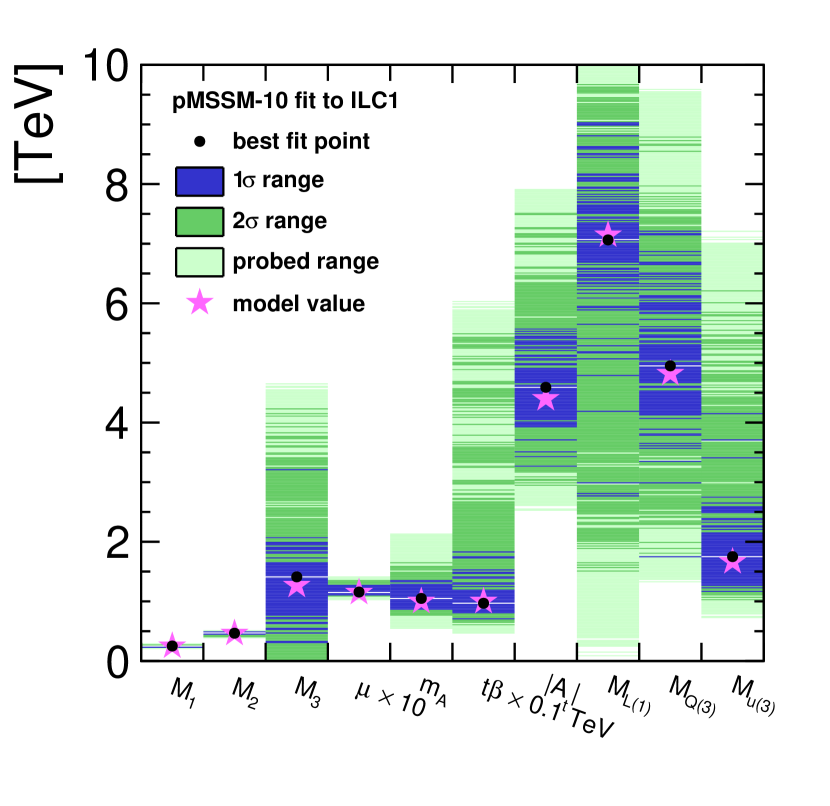
predictionILC1model valuebest fit1σ CL2σ CLmχ~30265.4267+816+1626mχ~40521.4524+2026+2655mχ~2±521.2524+1926+2555mH010011050+310190+610290mA010001050+310190+610290mH±10081056+304176+604276mu~L72297143+20374343+26575603mu~R72037117+20234337+26435577mt~119062003+1857763+3957803mt~249035033+23471993+39472653mb~148995028+23523188+39123488mb~272167130+20304310+26504470mg~15391693+18071273+28271693missing-subexpressionmissing-subexpressionmissing-subexpressionmissing-subexpressionmissing-subexpressionmissing-subexpressionmissing-subexpressionmissing-subexpressionmissing-subexpressionmissing-subexpressionpredictionILC1missing-subexpressionmodel valuebest fit1𝜎 CL2𝜎 CLmissing-subexpressionmissing-subexpressionmissing-subexpressionmissing-subexpressionmissing-subexpressionmissing-subexpressionmissing-subexpressionmissing-subexpressionmissing-subexpressionmissing-subexpressionsubscript𝑚superscriptsubscript~𝜒30265.4267superscriptsubscriptabsent168superscriptsubscriptabsent2616subscript𝑚superscriptsubscript~𝜒40521.4524superscriptsubscriptabsent2620superscriptsubscriptabsent5526subscript𝑚superscriptsubscript~𝜒2plus-or-minus521.2524superscriptsubscriptabsent2619superscriptsubscriptabsent5525subscript𝑚subscript𝐻010011050superscriptsubscriptabsent190310superscriptsubscriptabsent290610subscript𝑚subscript𝐴010001050superscriptsubscriptabsent190310superscriptsubscriptabsent290610subscript𝑚superscript𝐻plus-or-minus10081056superscriptsubscriptabsent176304superscriptsubscriptabsent276604subscript𝑚subscript~𝑢𝐿72297143superscriptsubscriptabsent43432037superscriptsubscriptabsent56032657subscript𝑚subscript~𝑢𝑅72037117superscriptsubscriptabsent43372023superscriptsubscriptabsent55772643subscript𝑚subscript~𝑡119062003superscriptsubscriptabsent7631857superscriptsubscriptabsent8033957subscript𝑚subscript~𝑡249035033superscriptsubscriptabsent19932347superscriptsubscriptabsent26533947subscript𝑚subscript~𝑏148995028superscriptsubscriptabsent31882352superscriptsubscriptabsent34883912subscript𝑚subscript~𝑏272167130superscriptsubscriptabsent43102030superscriptsubscriptabsent44702650subscript𝑚~𝑔15391693superscriptsubscriptabsent12731807superscriptsubscriptabsent16932827missing-subexpressionmissing-subexpressionmissing-subexpressionmissing-subexpressionmissing-subexpression\begin{array}[]{ c c c c c }\hline\cr\hline\cr\text{prediction}&\lx@intercol\hfil\text{ILC1}\hfil\lx@intercol\\ &\text{model value}&\text{best fit}&1\sigma\text{ CL}&2\sigma\text{ CL}\\ \hline\cr\hline\cr m_{\widetilde{\chi}_{3}^{0}}&265.4&267&\ {}_{-16}^{+8}&\ {}_{-26}^{+16}\\ m_{\widetilde{\chi}_{4}^{0}}&521.4&524&\ {}_{-26}^{+20}&\ {}_{-55}^{+26}\\ m_{\widetilde{\chi}_{2}^{\pm}}&521.2&524&\ {}_{-26}^{+19}&\ {}_{-55}^{+25}\\ m_{H_{0}}&1001&1050&\ {}_{-190}^{+310}&\ {}_{-290}^{+610}\\ m_{A_{0}}&1000&1050&\ {}_{-190}^{+310}&\ {}_{-290}^{+610}\\ m_{H^{\pm}}&1008&1056&\ {}_{-176}^{+304}&\ {}_{-276}^{+604}\\ m_{\widetilde{u}_{L}}&7229&7143&\ {}_{-4343}^{+2037}&\ {}_{-5603}^{+2657}\\ m_{\widetilde{u}_{R}}&7203&7117&\ {}_{-4337}^{+2023}&\ {}_{-5577}^{+2643}\\ m_{\widetilde{t}_{1}}&1906&2003&\ {}_{-763}^{+1857}&\ {}_{-803}^{+3957}\\ m_{\widetilde{t}_{2}}&4903&5033&\ {}_{-1993}^{+2347}&\ {}_{-2653}^{+3947}\\ m_{\widetilde{b}_{1}}&4899&5028&\ {}_{-3188}^{+2352}&\ {}_{-3488}^{+3912}\\ m_{\widetilde{b}_{2}}&7216&7130&\ {}_{-4310}^{+2030}&\ {}_{-4470}^{+2650}\\ m_{\widetilde{g}}&1539&1693&\ {}_{-1273}^{+1807}&\ {}_{-1693}^{+2827}\\ \hline\cr\hline\cr\end{array}

Table 16: True and fitted masses as well as their uncertainties from a pMSSM-10 fit to ILC1 observables. All values in GeV.
Refer to caption
(a) without gluino observation
Refer to caption
(b) with gluino observation
Figure 13: Predicted SUSY parameter ranges from the pMSSM-10 fit to ILC1. The magenta star indicates the true model values, while the black dot shows the best fit point.
Refer to caption
(a) without gluino observation
Refer to caption
(b) with gluino observation
Figure 14: Predicted mass ranges from the pMSSM-10 fit to ILC1. The green star indicates the true model values, while the black dot shows the best fit point.

Figure 15 illustrates the result of the corresponding pMSSM-4 fit with M1subscript𝑀1M_{1}, M2subscript𝑀2M_{2}, μ𝜇\mu and tanβ𝛽\tan\beta only. All four parameters can be determined accurately as also shown in Tab. 15. This results in predictions for the masses of the heavier electroweakinos with precisions between 1.6 and 3%.
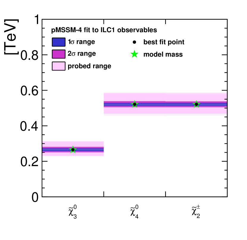
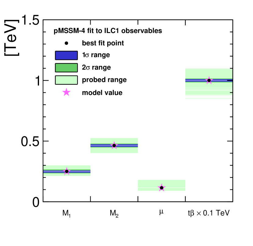
Refer to caption
(a) Fitted masses
Refer to caption
(b) Fitted parameters
Figure 15: Predicted mass and SUSY parameter ranges from the pMSSM-4 fit to ILC1. The green/magenta star indicates the true model values, while the black dot shows the best fit point.

5.2.2 ILC2 Benchmark

In the case of the ILC2 benchmark, the overall situation is similar to the case of ILC1. The minimum χ2superscript𝜒2\chi^{2} as a function of M1subscript𝑀1M_{1}, M2subscript𝑀2M_{2} and μ𝜇\mu and tanβ𝛽\tan\beta is displayed in Fig. 16 for the pMSSM-10 and pMSSM-4. However, this time the I20 running scenario was assumed, c.f. Sec. 4.3. Also here, the resulting curve for the 4-parameter fit is much smoother than for the 10-parameter version due to the much smaller parameter space to be sampled. Like for ILC1, the precision on M2subscript𝑀2M_{2} improves somewhat in the pMSSM-4 fit, while μ𝜇\mu and tanβ𝛽\tan{\beta} are significantly better constrained.
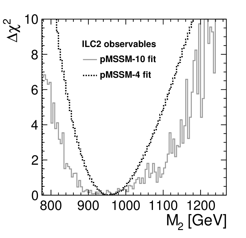
Refer to caption
(a)
Refer to caption
(b)
Refer to caption
(c)
Refer to caption
(d)
Figure 16: ILC2: Minimum χ2superscript𝜒2\chi^{2} as a function of M1subscript𝑀1M_{1}, M2subscript𝑀2M_{2} and μ𝜇\mu and tanβ𝛽\tan\beta in pMSSM-4 fit (dashed black line) and pMSSM-10 fit (solid grey line). For each bin, the minimum χ2superscript𝜒2\chi^{2} of all Markov chain points which have the x𝑥x axis quantity in that bin is plotted.

The resulting best fit values for the pMSSM parameters and their 1 and 2σ𝜎\sigma intervals are compared to the input values in Tab. 17, quantifying the effect which could already be seen qualitatively in Fig. 16. Again constraints on the sfermion sector can be derived due to their loop contributions. In contrast to the perfect agreement of the best fit point with the input parameter values in ILC1, the best fit point for ILC2 visibly overestimates the sfermion mass parameters. However the true values still remain within the 1σ𝜎\sigma interval. Figure 17(b) displays the precisions obtained on the pMSSM-10 parameters. In case of ILC2, the gluino is most likely outside the reach of LHC, therefore M3subscript𝑀3M_{3} is only constrained via its loop effects on the higgsino sector.
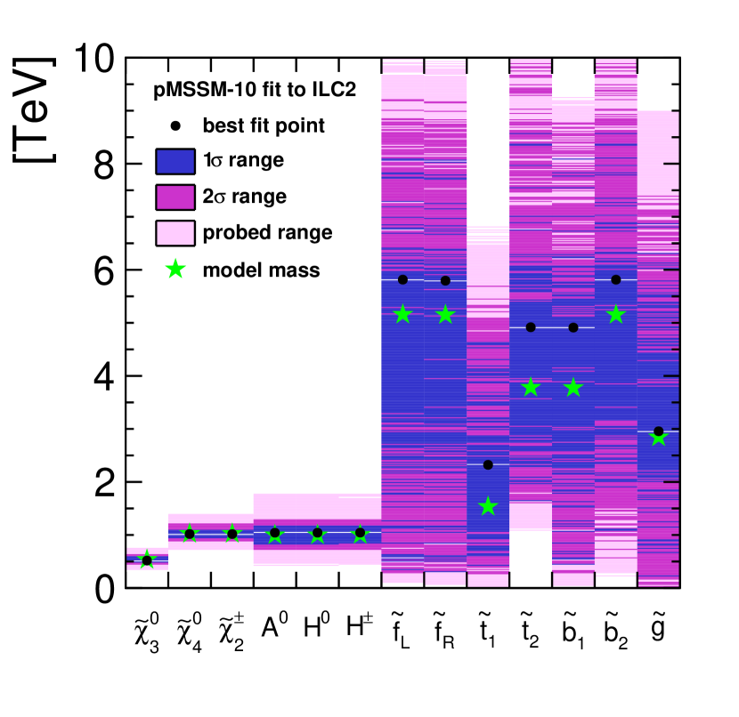
pMSSM-4pMSSM-10parameterILC2 pMSSM truebest fit point1σ CL2σ CLbest fit point1σ CL2σ CLM1520.3520.737.6+38.671.0+79.1502.132.9+91.371.7+130.1M2957.2959.4253.1+55.4100.1+124.1941.071.7+145.4130.9+229.2μ150.0150.00.4+0.40.8+0.7154.47.3+24.78.2+36.6tanβ15.015.00.6+0.71.2+1.714.87.8+38.49.0+48.2mA10001043203+135325+240M3260726842585+49902682+5670ML514657975359+24025544+3511MU(3)139520731805+35181805+4716MQ(3)375748713933+36804608+5030At471459483387+27344050+3250χ20.00260.1627missing-subexpressionmissing-subexpressionmissing-subexpressionmissing-subexpressionmissing-subexpressionmissing-subexpressionmissing-subexpressionmissing-subexpressionmissing-subexpressionmissing-subexpressionpMSSM-4missing-subexpressionmissing-subexpressionpMSSM-10missing-subexpressionmissing-subexpressionparameterILC2 pMSSM truebest fit point1𝜎 CL2𝜎 CLbest fit point1𝜎 CL2𝜎 CLmissing-subexpressionmissing-subexpressionmissing-subexpressionmissing-subexpressionmissing-subexpressionmissing-subexpressionmissing-subexpressionmissing-subexpressionmissing-subexpressionmissing-subexpressionmissing-subexpressionmissing-subexpressionmissing-subexpressionmissing-subexpressionmissing-subexpressionmissing-subexpressionsubscript𝑀1520.3520.7subscriptsuperscriptabsent38.637.6subscriptsuperscriptabsent79.171.0502.1subscriptsuperscriptabsent91.332.9subscriptsuperscriptabsent130.171.7subscript𝑀2957.2959.42subscriptsuperscriptabsent55.453.1subscriptsuperscriptabsent124.1100.1941.0subscriptsuperscriptabsent145.471.7subscriptsuperscriptabsent229.2130.9𝜇150.0150.0subscriptsuperscriptabsent0.40.4subscriptsuperscriptabsent0.70.8154.4subscriptsuperscriptabsent24.77.3subscriptsuperscriptabsent36.68.2𝛽15.015.0subscriptsuperscriptabsent0.70.6subscriptsuperscriptabsent1.71.214.8subscriptsuperscriptabsent38.47.8subscriptsuperscriptabsent48.29.0subscript𝑚𝐴1000missing-subexpressionmissing-subexpressionmissing-subexpression1043subscriptsuperscriptabsent135203subscriptsuperscriptabsent240325subscript𝑀32607missing-subexpressionmissing-subexpressionmissing-subexpression2684subscriptsuperscriptabsent49902585subscriptsuperscriptabsent56702682subscript𝑀𝐿5146missing-subexpressionmissing-subexpressionmissing-subexpression5797subscriptsuperscriptabsent24025359subscriptsuperscriptabsent35115544subscript𝑀𝑈31395missing-subexpressionmissing-subexpressionmissing-subexpression2073subscriptsuperscriptabsent35181805subscriptsuperscriptabsent47161805subscript𝑀𝑄33757missing-subexpressionmissing-subexpressionmissing-subexpression4871subscriptsuperscriptabsent36803933subscriptsuperscriptabsent50304608subscript𝐴𝑡4714missing-subexpressionmissing-subexpressionmissing-subexpression5948subscriptsuperscriptabsent27343387subscriptsuperscriptabsent32504050missing-subexpressionmissing-subexpressionmissing-subexpressionmissing-subexpressionmissing-subexpressionmissing-subexpressionmissing-subexpressionmissing-subexpressionsuperscript𝜒2missing-subexpression0.0026missing-subexpressionmissing-subexpression0.1627missing-subexpressionmissing-subexpressionmissing-subexpressionmissing-subexpressionmissing-subexpressionmissing-subexpressionmissing-subexpressionmissing-subexpressionmissing-subexpressionmissing-subexpression\begin{array}[]{ c c | c c c | c c c }\hline\cr&&\text{pMSSM-4}&&&\text{pMSSM-10}&&\\ \text{parameter}&\text{ILC2 pMSSM true}&\text{best fit point}&1\sigma\text{ CL}&2\sigma\text{ CL}&\text{best fit point}&1\sigma\text{ CL}&2\sigma\text{ CL}\\ \hline\cr\hline\cr M_{1}&520.3&520.7&\ {}^{+38.6}_{-37.6}&\ {}^{+79.1}_{-71.0}&502.1&\ {}^{+91.3}_{-32.9}&\ {}^{+130.1}_{-71.7}\\ M_{2}&957.2&959.42&\ {}^{+55.4}_{-53.1}&\ {}^{+124.1}_{-100.1}&941.0&\ {}^{+145.4}_{-71.7}&\ {}^{+229.2}_{-130.9}\\ \mu&150.0&150.0&\ {}^{+0.4}_{-0.4}&\ {}^{+0.7}_{-0.8}&154.4&\ {}^{+24.7}_{-7.3}&\ {}^{+36.6}_{-8.2}\\ \tan\beta&15.0&15.0&\ {}^{+0.7}_{-0.6}&\ {}^{+1.7}_{-1.2}&14.8&\ {}^{+38.4}_{-7.8}&\ {}^{+48.2}_{-9.0}\\ m_{A}&1000&&&&1043&\ {}^{+135}_{-203}&\ {}^{+240}_{-325}\\ M_{3}&2607&&&&2684&\ {}^{+4990}_{-2585}&\ {}^{+5670}_{-2682}\\ M_{L}&5146&&&&5797&\ {}^{+2402}_{-5359}&\ {}^{+3511}_{-5544}\\ M_{U(3)}&1395&&&&2073&\ {}^{+3518}_{-1805}&\ {}^{+4716}_{-1805}\\ M_{Q(3)}&3757&&&&4871&\ {}^{+3680}_{-3933}&\ {}^{+5030}_{-4608}\\ A_{t}&-4714&&&&-5948&\ {}^{+2734}_{-3387}&\ {}^{+3250}_{-4050}\\ \hline\cr\chi^{2}&&0.0026&&&0.1627&&\\ \hline\cr\hline\cr\end{array}

Table 17: Fitted parameters in ILC2 pMSSM-4 and pMSSM-10. All units in GeV except for tanβ𝛽\tan\beta and χ2superscript𝜒2\chi^{2}.

predictionILC2model massesbest fit1σ2σmχ~30534.6518+7234+11074mχ~4010261018+8276+190134mχ~2±10261018+8276+190134mH010001043+137223+257323mA010001043+137223+257323mH±10031045+135205+255325mu~L51585814+22865474+34065534mu~R51435795+22855495+33855495mt~115352322+23181902+33782062mt~237824917+36633277+49833317mb~137744911+31894471+38694631mb~251545814+27664734+40865254mg~28462955+39252735+44452935missing-subexpressionmissing-subexpressionmissing-subexpressionmissing-subexpressionmissing-subexpressionmissing-subexpressionmissing-subexpressionmissing-subexpressionmissing-subexpressionmissing-subexpressionpredictionILC2missing-subexpressionmodel massesbest fit1𝜎2𝜎missing-subexpressionmissing-subexpressionmissing-subexpressionmissing-subexpressionmissing-subexpressionmissing-subexpressionmissing-subexpressionmissing-subexpressionmissing-subexpressionmissing-subexpressionsubscript𝑚superscriptsubscript~𝜒30534.6518superscriptsubscriptabsent3472superscriptsubscriptabsent74110subscript𝑚superscriptsubscript~𝜒4010261018superscriptsubscriptabsent7682superscriptsubscriptabsent134190subscript𝑚superscriptsubscript~𝜒2plus-or-minus10261018superscriptsubscriptabsent7682superscriptsubscriptabsent134190subscript𝑚subscript𝐻010001043superscriptsubscriptabsent223137superscriptsubscriptabsent323257subscript𝑚subscript𝐴010001043superscriptsubscriptabsent223137superscriptsubscriptabsent323257subscript𝑚superscript𝐻plus-or-minus10031045superscriptsubscriptabsent205135superscriptsubscriptabsent325255subscript𝑚subscript~𝑢𝐿51585814superscriptsubscriptabsent54742286superscriptsubscriptabsent55343406subscript𝑚subscript~𝑢𝑅51435795superscriptsubscriptabsent54952285superscriptsubscriptabsent54953385subscript𝑚subscript~𝑡115352322superscriptsubscriptabsent19022318superscriptsubscriptabsent20623378subscript𝑚subscript~𝑡237824917superscriptsubscriptabsent32773663superscriptsubscriptabsent33174983subscript𝑚subscript~𝑏137744911superscriptsubscriptabsent44713189superscriptsubscriptabsent46313869subscript𝑚subscript~𝑏251545814superscriptsubscriptabsent47342766superscriptsubscriptabsent52544086subscript𝑚~𝑔28462955superscriptsubscriptabsent27353925superscriptsubscriptabsent29354445missing-subexpressionmissing-subexpressionmissing-subexpressionmissing-subexpressionmissing-subexpression\begin{array}[]{ c c c c c }\hline\cr\hline\cr\text{prediction}&\lx@intercol\hfil\text{ILC2}\hfil\lx@intercol\\ &\text{model masses}&\text{best fit}&1\sigma&2\sigma\\ \hline\cr\hline\cr m_{\widetilde{\chi}_{3}^{0}}&534.6&518&\ {}_{-34}^{+72}&\ {}_{-74}^{+110}\\ m_{\widetilde{\chi}_{4}^{0}}&1026&1018&\ {}_{-76}^{+82}&\ {}_{-134}^{+190}\\ m_{\widetilde{\chi}_{2}^{\pm}}&1026&1018&\ {}_{-76}^{+82}&\ {}_{-134}^{+190}\\ m_{H_{0}}&1000&1043&\ {}_{-223}^{+137}&\ {}_{-323}^{+257}\\ m_{A_{0}}&1000&1043&\ {}_{-223}^{+137}&\ {}_{-323}^{+257}\\ m_{H^{\pm}}&1003&1045&\ {}_{-205}^{+135}&\ {}_{-325}^{+255}\\ m_{\widetilde{u}_{L}}&5158&5814&\ {}_{-5474}^{+2286}&\ {}_{-5534}^{+3406}\\ m_{\widetilde{u}_{R}}&5143&5795&\ {}_{-5495}^{+2285}&\ {}_{-5495}^{+3385}\\ m_{\widetilde{t}_{1}}&1535&2322&\ {}_{-1902}^{+2318}&\ {}_{-2062}^{+3378}\\ m_{\widetilde{t}_{2}}&3782&4917&\ {}_{-3277}^{+3663}&\ {}_{-3317}^{+4983}\\ m_{\widetilde{b}_{1}}&3774&4911&\ {}_{-4471}^{+3189}&\ {}_{-4631}^{+3869}\\ m_{\widetilde{b}_{2}}&5154&5814&\ {}_{-4734}^{+2766}&\ {}_{-5254}^{+4086}\\ m_{\widetilde{g}}&2846&2955&\ {}_{-2735}^{+3925}&\ {}_{-2935}^{+4445}\\ \hline\cr\hline\cr\end{array}

Table 18: True and fitted masses as well as their uncertainties from a pMSSM-10 fit to ILC2 observables. All values in GeV.
Refer to caption
(a) Fitted masses
Refer to caption
(b) Fitted parameters
Figure 17: Predicted mass and SUSY parameter ranges from the pMSSM-10 fit to ILC2. The green/magenta star indicates the true model values, while the black dot shows the best fit point.

As in the ILC1 case, the determined parameters can be used to predict the masses of the as-yet unobserved sparticles, as shown for the pMSSM-10 fit in Tab. 18 and Fig. 17(a). Finally, Fig. 18(a) shows the result of the 4 parameter fit of M1subscript𝑀1M_{1}, M2subscript𝑀2M_{2}, μ𝜇\mu, tanβ𝛽\tan\beta. Again, the remaining parameters fixed to model values, based on the assumption that the best fit point of the 10-parameter fit is sufficiently close to the true point that the effect of fixing to the true values is negligible.
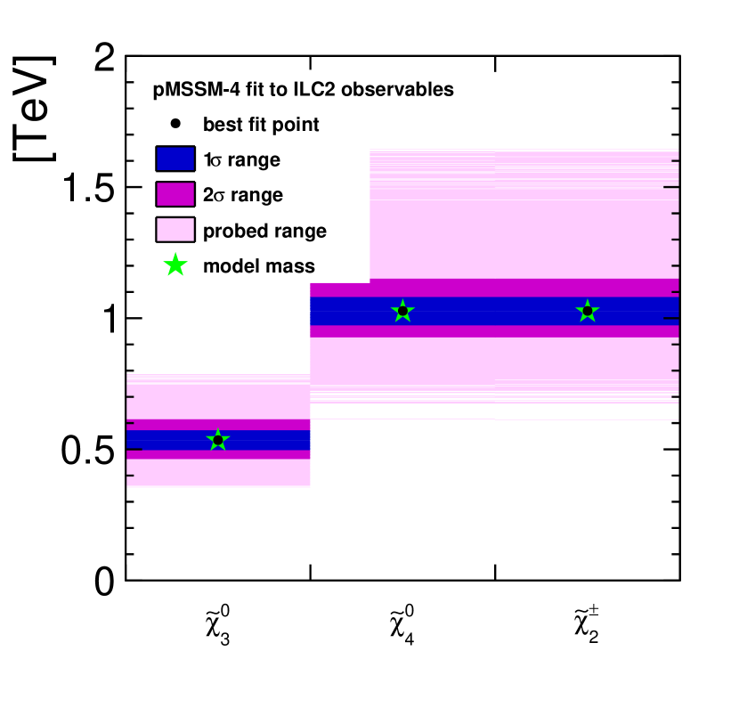
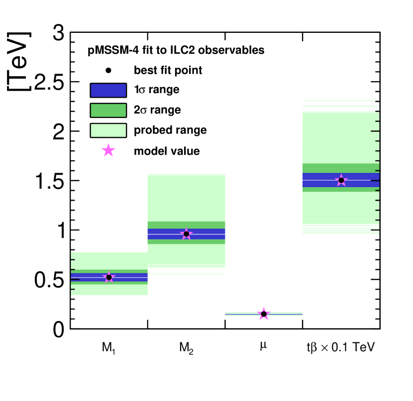
Refer to caption
(a) Fitted masses
Refer to caption
(b) Fitted parameters
Figure 18: Predicted mass and SUSY parameter ranges from the pMSSM-4 fit to ILC2. The green/magenta star indicates the true model values, while the black dot shows the best fit point.

5.2.3 nGMM1 Benchmark

Finally, Fig. 19 shows the minimum χ2superscript𝜒2\chi^{2} as a function of M1subscript𝑀1M_{1}, M2subscript𝑀2M_{2} and μ𝜇\mu and tanβ𝛽\tan\beta in the pMSSM-10 and pMSSM-4 fits to the nGMM1 observables. Also here, the much smaller parameter space to be sampled in case of the 4-dimensional fit leads to much smoother curves than in the 10-dimensional case. Again, the determinations of μ𝜇\mu and tanβ𝛽\tan{\beta} improve significantly. However M1subscript𝑀1M_{1} and M2subscript𝑀2M_{2} exchange their roles compared to the other benchmarks, so that now M1subscript𝑀1M_{1} is somewhat better constrained in the pMSSM-4 fit, while the precision on M2subscript𝑀2M_{2} is nearly identical in the two fits. However, it should be noted that M1subscript𝑀1M_{1} and M2subscript𝑀2M_{2} are less well constrained than in the cases of the ILC1 and ILC2 benchmarks. This results from a combination of the worse experimental resolutions and the larger absolute values of M1subscript𝑀1M_{1} and M2subscript𝑀2M_{2} in case of nGMM1. In this most challenging case, the mass splitting between χ~1±superscriptsubscript~𝜒1plus-or-minus\widetilde{\chi}_{1}^{\pm} and χ~10superscriptsubscript~𝜒10\widetilde{\chi}_{1}^{0} is only 2.5 GeV, which corresponds to less than 2σ𝜎\sigma of the experimental resolution. As discussed in Sec. 3.3, the mass differences mχ~20mχ~10subscript𝑚superscriptsubscript~𝜒20subscript𝑚superscriptsubscript~𝜒10m_{\widetilde{\chi}_{2}^{0}}-m_{\widetilde{\chi}_{1}^{0}} and mχ~1±mχ~10subscript𝑚superscriptsubscript~𝜒1plus-or-minussubscript𝑚superscriptsubscript~𝜒10m_{\widetilde{\chi}_{1}^{\pm}}-m_{\widetilde{\chi}_{1}^{0}} are directly accessible experimentally as the endpoint of the di-lepton or di-jet invariant mass spectrum. Therefore, we consider in this case as alternative input these mass differences in addition to the χ~10superscriptsubscript~𝜒10\widetilde{\chi}_{1}^{0} mass, which also presents a set of observables with minimal correlations. The corresponding precisions are summarized in Tab. 19.
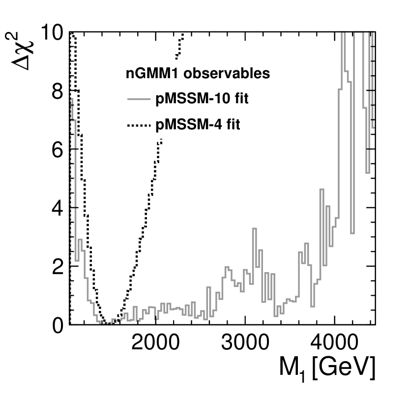
observablenGMM1 model value [GeV]precisionI20 precisionmχ~10154.91.7%1.0%mχ~20mχ~105.32.1%1.4%mχ~1±mχ~102.42.5%1.2%missing-subexpressionmissing-subexpressionmissing-subexpressionmissing-subexpressionmissing-subexpressionmissing-subexpressionmissing-subexpressionmissing-subexpressionobservablenGMM1 model value [GeV]precisionI20 precisionmissing-subexpressionmissing-subexpressionmissing-subexpressionmissing-subexpressionsubscript𝑚superscriptsubscript~𝜒10154.9percent1.7percent1.0subscript𝑚superscriptsubscript~𝜒20subscript𝑚superscriptsubscript~𝜒105.3percent2.1percent1.4subscript𝑚superscriptsubscript~𝜒1plus-or-minussubscript𝑚superscriptsubscript~𝜒102.4percent2.5percent1.2missing-subexpressionmissing-subexpressionmissing-subexpressionmissing-subexpression\begin{array}[]{ c c c c }\hline\cr\hline\cr\text{observable}&\text{nGMM1 model value [GeV]}&\text{precision}&\text{I20 precision}\\ \hline\cr m_{\widetilde{\chi}_{1}^{0}}&154.9&1.7\%&1.0\%\\ m_{\widetilde{\chi}_{2}^{0}}-m_{\widetilde{\chi}_{1}^{0}}&5.3&2.1\%&1.4\%\\ m_{\widetilde{\chi}_{1}^{\pm}}-m_{\widetilde{\chi}_{1}^{0}}&2.4&2.5\%&1.2\%\\ \hline\cr\hline\cr\end{array}

Table 19: Experimental precision on the higgsino mass differences in nGMM1 combined from 500 GeV 500-1 fb for both 𝒫(±0.8,0.3)𝒫plus-or-minus0.8minus-or-plus0.3\mathcal{P}(\pm 0.8,\mp 0.3), as well as scaled to 1600 fb-1 for both polarisations at s=500 GeV𝑠500 GeV\sqrt{s}=500\text{ GeV}, ignoring the data sets with other centre-of-mass energies in the I20 operating scenario. Again, it is assumed that the precisions obtained from the simulations based on the Isajet spectrum can be transfered to the SPheno3.3.9beta spectrum.
Refer to caption
(a)
Refer to caption
(b)
Refer to caption
(c)
Refer to caption
(d)
Figure 19: nGMM1: Minimum χ2superscript𝜒2\chi^{2} as a function of M1subscript𝑀1M_{1}, M2subscript𝑀2M_{2} and μ𝜇\mu and tanβ𝛽\tan\beta in pMSSM-4 fit (dashed black line) and pMSSM-10 fit (solid grey line). For each bin, the minimum χ2superscript𝜒2\chi^{2} of all Markov chain points which have the x𝑥x axis quantity in that bin is plotted.
Refer to caption
Figure 20: nGMM1 χ2superscript𝜒2\chi^{2} parabola for M2subscript𝑀2M_{2} in the 10-parameter fit with mass differences (black, dashed) and the same fit with masses as observables (grey, solid).

As can be seen in Fig. 20, the determination of M2subscript𝑀2M_{2} in the 10-parameter fit improves significantly when instead of the absolute masses the mass differences are used as fit input, especially the upper bound. There is no significant effect on M1subscript𝑀1M_{1}, μ𝜇\mu or tanβ𝛽\tan\beta.

The resulting best fit values for the pMSSM parameters and their 1 and 2σ𝜎\sigma intervals are compared to the input values in Tab. 20, quantifying the effect which could already be seen qualitatively in Fig’s. 19 and 20. As before, constraints on the sfermion sector can be derived due to their loop contributions. In contrast to the perfect agreement of the best fit point with the input parameter values in ILC1, the best fit point for nGMM1 visibly overestimates the sfermion mass parameters. However the true values still remain within the 1σ𝜎\sigma interval. Using the mass differences as input instead of the absolute higgsino masses notably improves the precision on M2subscript𝑀2M_{2}, as expected from the χ2superscript𝜒2\chi^{2} distribution, but it also significantly improves the agreement of the best fit point with the true model parameters. These improvements can also be seen in Fig. 21(b) and 21(d), in particular the better agreement in mAsubscript𝑚𝐴m_{A} and Atsubscript𝐴𝑡A_{t}.

pMSSM-4pMSSM-10pMSSM-10 with mass differencesparametertruebest fit point1σ CL2σ CLbest fit point1σ CL2σ CLbest fit point1σ CL2σ CLM114931501149+173280+4111386145+2386282+28301573282+2091344+5650M217201711158+220279+5301768451+254549+7171710313+137394+277μ150.0150.00.4+0.40.9+0.9154.28.7+7.48.3+12.9149.93.4+11.54.2+15.3tanβ10.010.00.3+0.50.6+1.28.31.3+41.91.9+44.611.23.4+32.54.2+63.9mA200026551449+64931596+114921868567+4018867+6423M3264631733168+42293168+534726772541+38922614+4550ML511547814077+35894456+463054124581+16295118+2319MU(3)138117741086+23841214+4826996500+3540741+4686MQ(3)370140113535+32543697+398238743245+19833370+2356At48576766509+36981702+401245824006+15584390+1750χ20.01380.09270.0668missing-subexpressionmissing-subexpressionmissing-subexpressionmissing-subexpressionmissing-subexpressionmissing-subexpressionmissing-subexpressionmissing-subexpressionmissing-subexpressionmissing-subexpressionmissing-subexpressionmissing-subexpressionmissing-subexpressionpMSSM-4pMSSM-10pMSSM-10 with mass differencesparametertruebest fit point1𝜎 CL2𝜎 CLbest fit point1𝜎 CL2𝜎 CLbest fit point1𝜎 CL2𝜎 CLmissing-subexpressionmissing-subexpressionmissing-subexpressionmissing-subexpressionmissing-subexpressionmissing-subexpressionmissing-subexpressionmissing-subexpressionmissing-subexpressionmissing-subexpressionmissing-subexpressionmissing-subexpressionmissing-subexpressionmissing-subexpressionmissing-subexpressionmissing-subexpressionmissing-subexpressionmissing-subexpressionmissing-subexpressionmissing-subexpressionmissing-subexpressionmissing-subexpressionsubscript𝑀114931501subscriptsuperscriptabsent173149subscriptsuperscriptabsent4112801386subscriptsuperscriptabsent2386145subscriptsuperscriptabsent28302821573subscriptsuperscriptabsent2091282subscriptsuperscriptabsent5650344subscript𝑀217201711subscriptsuperscriptabsent220158subscriptsuperscriptabsent5302791768subscriptsuperscriptabsent254451subscriptsuperscriptabsent7175491710subscriptsuperscriptabsent137313subscriptsuperscriptabsent277394𝜇150.0150.0subscriptsuperscriptabsent0.40.4subscriptsuperscriptabsent0.90.9154.2subscriptsuperscriptabsent7.48.7subscriptsuperscriptabsent12.98.3149.9subscriptsuperscriptabsent11.53.4subscriptsuperscriptabsent15.34.2𝛽10.010.0subscriptsuperscriptabsent0.50.3subscriptsuperscriptabsent1.20.68.3subscriptsuperscriptabsent41.91.3subscriptsuperscriptabsent44.61.911.2subscriptsuperscriptabsent32.53.4subscriptsuperscriptabsent63.94.2subscript𝑚𝐴2000missing-subexpressionmissing-subexpressionmissing-subexpression2655subscriptsuperscriptabsent64931449subscriptsuperscriptabsent1149215961868subscriptsuperscriptabsent4018567subscriptsuperscriptabsent6423867subscript𝑀32646missing-subexpressionmissing-subexpressionmissing-subexpression3173subscriptsuperscriptabsent42293168subscriptsuperscriptabsent534731682677subscriptsuperscriptabsent38922541subscriptsuperscriptabsent45502614subscript𝑀𝐿5115missing-subexpressionmissing-subexpressionmissing-subexpression4781subscriptsuperscriptabsent35894077subscriptsuperscriptabsent463044565412subscriptsuperscriptabsent16294581subscriptsuperscriptabsent23195118subscript𝑀𝑈31381missing-subexpressionmissing-subexpressionmissing-subexpression1774subscriptsuperscriptabsent23841086subscriptsuperscriptabsent48261214996subscriptsuperscriptabsent3540500subscriptsuperscriptabsent4686741subscript𝑀𝑄33701missing-subexpressionmissing-subexpressionmissing-subexpression4011subscriptsuperscriptabsent32543535subscriptsuperscriptabsent398236973874subscriptsuperscriptabsent19833245subscriptsuperscriptabsent23563370subscript𝐴𝑡4857missing-subexpressionmissing-subexpressionmissing-subexpression6766subscriptsuperscriptabsent3698509subscriptsuperscriptabsent401217024582subscriptsuperscriptabsent15584006subscriptsuperscriptabsent17504390missing-subexpressionmissing-subexpressionmissing-subexpressionmissing-subexpressionmissing-subexpressionmissing-subexpressionmissing-subexpressionmissing-subexpressionmissing-subexpressionmissing-subexpressionmissing-subexpressionsuperscript𝜒2missing-subexpression0.0138missing-subexpressionmissing-subexpression0.0927missing-subexpressionmissing-subexpression0.0668missing-subexpressionmissing-subexpressionmissing-subexpressionmissing-subexpressionmissing-subexpressionmissing-subexpressionmissing-subexpressionmissing-subexpressionmissing-subexpressionmissing-subexpressionmissing-subexpressionmissing-subexpressionmissing-subexpression\begin{array}[]{ c c | c c c | c c c | c c c }\hline\cr&&\lx@intercol\hfil\text{pMSSM-4}\hfil\lx@intercol\vrule\lx@intercol&\lx@intercol\hfil\text{pMSSM-10}\hfil\lx@intercol\vrule\lx@intercol&\lx@intercol\hfil\text{pMSSM-10 with mass differences}\hfil\lx@intercol\\ \text{parameter}&\text{true}&\text{best fit point}&1\sigma\text{ CL}&2\sigma\text{ CL}&\text{best fit point}&1\sigma\text{ CL}&2\sigma\text{ CL}&\text{best fit point}&1\sigma\text{ CL}&2\sigma\text{ CL}\\ \hline\cr\hline\cr M_{1}&1493&1501&\ {}^{+173}_{-149}&\ {}^{+411}_{-280}&1386&\ {}^{+2386}_{-145}&\ {}^{+2830}_{-282}&1573&\ {}^{+2091}_{-282}&\ {}^{+5650}_{-344}\\ M_{2}&1720&1711&\ {}^{+220}_{-158}&\ {}^{+530}_{-279}&1768&\ {}^{+254}_{-451}&\ {}^{+717}_{-549}&1710&\ {}^{+137}_{-313}&\ {}^{+277}_{-394}\\ \mu&150.0&150.0&\ {}^{+0.4}_{-0.4}&\ {}^{+0.9}_{-0.9}&154.2&\ {}^{+7.4}_{-8.7}&\ {}^{+12.9}_{-8.3}&149.9&\ {}^{+11.5}_{-3.4}&\ {}^{+15.3}_{-4.2}\\ \tan\beta&10.0&10.0&\ {}^{+0.5}_{-0.3}&\ {}^{+1.2}_{-0.6}&8.3&\ {}^{+41.9}_{-1.3}&\ {}^{+44.6}_{-1.9}&11.2&\ {}^{+32.5}_{-3.4}&\ {}^{+63.9}_{-4.2}\\ m_{A}&2000&&&&2655&\ {}^{+6493}_{-1449}&\ {}^{+11492}_{-1596}&1868&\ {}^{+4018}_{-567}&\ {}^{+6423}_{-867}\\ M_{3}&2646&&&&3173&\ {}^{+4229}_{-3168}&\ {}^{+5347}_{-3168}&2677&\ {}^{+3892}_{-2541}&\ {}^{+4550}_{-2614}\\ M_{L}&5115&&&&4781&\ {}^{+3589}_{-4077}&\ {}^{+4630}_{-4456}&5412&\ {}^{+1629}_{-4581}&\ {}^{+2319}_{-5118}\\ M_{U(3)}&1381&&&&1774&\ {}^{+2384}_{-1086}&\ {}^{+4826}_{-1214}&996&\ {}^{+3540}_{-500}&\ {}^{+4686}_{-741}\\ M_{Q(3)}&3701&&&&4011&\ {}^{+3254}_{-3535}&\ {}^{+3982}_{-3697}&3874&\ {}^{+1983}_{-3245}&\ {}^{+2356}_{-3370}\\ A_{t}&-4857&&&&-6766&\ {}^{+3698}_{-509}&\ {}^{+4012}_{-1702}&-4582&\ {}^{+1558}_{-4006}&\ {}^{+1750}_{-4390}\\ \hline\cr\chi^{2}&&0.0138&&&0.0927&&&0.0668&&\\ \hline\cr\hline\cr\end{array}

Table 20: Fitted parameters in nGMM1: pMSSM-4, pMSSM-10 and pMSSM-10 with mass differences as input. All units in GeV except for tanβ𝛽\tan\beta and χ2superscript𝜒2\chi^{2}.

predictionnGMM1MnGMM1ΔMmodel massbest fit1σ2σbest fit1σ2σmχ~3015221412+454134+6402601603+149283+347349mχ~4018091854+1920264+23643361802+1834146+2710218mχ~2±18081853+229443+6015571801+137349+275433mH020002655+63651355+712515551868+3992528+6372828mA020002655+63651355+712515551868+3992528+6372828mH±20022656+63641336+712415561863+3997523+6377823mu~L51214762+36984282+471845825421+16194721+22395221mu~R51104754+36664294+470645945408+16124708+22325108mt~115191951+15491411+388914711168+3332548+3332868mt~237824029+31202160+390025203894+20262014+23262394mb~137744008+28523448+371237483888+20323168+22323528mb~251544763+36973703+471742635419+16214599+22414739mg~28463361+32593261+455933612924+29762684+35562804missing-subexpressionmissing-subexpressionmissing-subexpressionmissing-subexpressionmissing-subexpressionmissing-subexpressionmissing-subexpressionmissing-subexpressionmissing-subexpressionmissing-subexpressionmissing-subexpressionmissing-subexpressionmissing-subexpressionmissing-subexpressionmissing-subexpressionmissing-subexpressionpredictionnGMM1𝑀nGMM1Δ𝑀missing-subexpressionmissing-subexpressionmodel massbest fit1𝜎2𝜎best fit1𝜎2𝜎missing-subexpressionmissing-subexpressionmissing-subexpressionmissing-subexpressionmissing-subexpressionmissing-subexpressionmissing-subexpressionmissing-subexpressionmissing-subexpressionmissing-subexpressionmissing-subexpressionmissing-subexpressionmissing-subexpressionmissing-subexpressionmissing-subexpressionmissing-subexpressionmissing-subexpressionsubscript𝑚superscriptsubscript~𝜒3015221412superscriptsubscriptabsent134454superscriptsubscriptabsent2606401603superscriptsubscriptabsent283149superscriptsubscriptabsent349347subscript𝑚superscriptsubscript~𝜒4018091854superscriptsubscriptabsent2641920superscriptsubscriptabsent33623641802superscriptsubscriptabsent1461834superscriptsubscriptabsent2182710subscript𝑚superscriptsubscript~𝜒2plus-or-minus18081853superscriptsubscriptabsent443229superscriptsubscriptabsent5576011801superscriptsubscriptabsent349137superscriptsubscriptabsent433275subscript𝑚subscript𝐻020002655superscriptsubscriptabsent13556365superscriptsubscriptabsent155571251868superscriptsubscriptabsent5283992superscriptsubscriptabsent8286372subscript𝑚subscript𝐴020002655superscriptsubscriptabsent13556365superscriptsubscriptabsent155571251868superscriptsubscriptabsent5283992superscriptsubscriptabsent8286372subscript𝑚superscript𝐻plus-or-minus20022656superscriptsubscriptabsent13366364superscriptsubscriptabsent155671241863superscriptsubscriptabsent5233997superscriptsubscriptabsent8236377subscript𝑚subscript~𝑢𝐿51214762superscriptsubscriptabsent42823698superscriptsubscriptabsent458247185421superscriptsubscriptabsent47211619superscriptsubscriptabsent52212239subscript𝑚subscript~𝑢𝑅51104754superscriptsubscriptabsent42943666superscriptsubscriptabsent459447065408superscriptsubscriptabsent47081612superscriptsubscriptabsent51082232subscript𝑚subscript~𝑡115191951superscriptsubscriptabsent14111549superscriptsubscriptabsent147138891168superscriptsubscriptabsent5483332superscriptsubscriptabsent8683332subscript𝑚subscript~𝑡237824029superscriptsubscriptabsent21603120superscriptsubscriptabsent252039003894superscriptsubscriptabsent20142026superscriptsubscriptabsent23942326subscript𝑚subscript~𝑏137744008superscriptsubscriptabsent34482852superscriptsubscriptabsent374837123888superscriptsubscriptabsent31682032superscriptsubscriptabsent35282232subscript𝑚subscript~𝑏251544763superscriptsubscriptabsent37033697superscriptsubscriptabsent426347175419superscriptsubscriptabsent45991621superscriptsubscriptabsent47392241subscript𝑚~𝑔28463361superscriptsubscriptabsent32613259superscriptsubscriptabsent336145592924superscriptsubscriptabsent26842976superscriptsubscriptabsent28043556missing-subexpressionmissing-subexpressionmissing-subexpressionmissing-subexpressionmissing-subexpressionmissing-subexpressionmissing-subexpressionmissing-subexpression\begin{array}[]{ c c | c c c | c c c }\hline\cr\hline\cr\text{prediction}&\lx@intercol\hfil\text{nGMM1}M\hfil\lx@intercol\vrule\lx@intercol&\lx@intercol\hfil\text{nGMM1}\Delta M\hfil\lx@intercol\\ &\text{model mass}\text{best fit}&1\sigma&2\sigma&\text{best fit}&1\sigma&2\sigma\\ \hline\cr\hline\cr m_{\widetilde{\chi}_{3}^{0}}&1522&1412&\ {}_{-134}^{+454}&\ {}_{-260}^{+640}&1603&\ {}_{-283}^{+149}&\ {}_{-349}^{+347}\\ m_{\widetilde{\chi}_{4}^{0}}&1809&1854&\ {}_{-264}^{+1920}&\ {}_{-336}^{+2364}&1802&\ {}_{-146}^{+1834}&\ {}_{-218}^{+2710}\\ m_{\widetilde{\chi}_{2}^{\pm}}&1808&1853&\ {}_{-443}^{+229}&\ {}_{-557}^{+601}&1801&\ {}_{-349}^{+137}&\ {}_{-433}^{+275}\\ m_{H_{0}}&2000&2655&\ {}_{-1355}^{+6365}&\ {}_{-1555}^{+7125}&1868&\ {}_{-528}^{+3992}&\ {}_{-828}^{+6372}\\ m_{A_{0}}&2000&2655&\ {}_{-1355}^{+6365}&\ {}_{-1555}^{+7125}&1868&\ {}_{-528}^{+3992}&\ {}_{-828}^{+6372}\\ m_{H^{\pm}}&2002&2656&\ {}_{-1336}^{+6364}&\ {}_{-1556}^{+7124}&1863&\ {}_{-523}^{+3997}&\ {}_{-823}^{+6377}\\ m_{\widetilde{u}_{L}}&5121&4762&\ {}_{-4282}^{+3698}&\ {}_{-4582}^{+4718}&5421&\ {}_{-4721}^{+1619}&\ {}_{-5221}^{+2239}\\ m_{\widetilde{u}_{R}}&5110&4754&\ {}_{-4294}^{+3666}&\ {}_{-4594}^{+4706}&5408&\ {}_{-4708}^{+1612}&\ {}_{-5108}^{+2232}\\ m_{\widetilde{t}_{1}}&1519&1951&\ {}_{-1411}^{+1549}&\ {}_{-1471}^{+3889}&1168&\ {}_{-548}^{+3332}&\ {}_{-868}^{+3332}\\ m_{\widetilde{t}_{2}}&3782&4029&\ {}_{-2160}^{+3120}&\ {}_{-2520}^{+3900}&3894&\ {}_{-2014}^{+2026}&\ {}_{-2394}^{+2326}\\ m_{\widetilde{b}_{1}}&3774&4008&\ {}_{-3448}^{+2852}&\ {}_{-3748}^{+3712}&3888&\ {}_{-3168}^{+2032}&\ {}_{-3528}^{+2232}\\ m_{\widetilde{b}_{2}}&5154&4763&\ {}_{-3703}^{+3697}&\ {}_{-4263}^{+4717}&5419&\ {}_{-4599}^{+1621}&\ {}_{-4739}^{+2241}\\ m_{\widetilde{g}}&2846&3361&\ {}_{-3261}^{+3259}&\ {}_{-3361}^{+4559}&2924&\ {}_{-2684}^{+2976}&\ {}_{-2804}^{+3556}\\ \hline\cr\hline\cr\end{array}

Table 21: nGMM1: True and fitted masses and their uncertainties from pMSSM-10 fits with the standard set of observables as well as with the higgsino mass differences replacing the χ~20superscriptsubscript~𝜒20\widetilde{\chi}_{2}^{0} and χ~1±superscriptsubscript~𝜒1plus-or-minus\widetilde{\chi}_{1}^{\pm} masses as observables. All values in GeV.
Refer to caption
(a) Fitted masses, standard input
Refer to caption
(b) Fitted parameters, standard input
Refer to caption
(c) Fitted masses, mass difference input
Refer to caption
(d) Fitted parameters, mass difference input
Figure 21: Predicted mass and SUSY parameter ranges from the pMSSM-10 fit to nGMM1 observables - including either χ~20superscriptsubscript~𝜒20\widetilde{\chi}_{2}^{0} and χ~1±superscriptsubscript~𝜒1plus-or-minus\widetilde{\chi}_{1}^{\pm} masses or their mass differences with the LSP. The green/magenta star indicates the true model values, while the black dot shows the best fit point.

Again, the determined parameters can be used to predict the masses of the yet unobserved sparticles, as shown for the pMSSM-10 fit in Tab. 21 and in Fig. 21(a) and 21(c) with standard input and when using the mass differences instead. As expected, the improved precision on M2subscript𝑀2M_{2} when using the mass differences as input leads to improved predictions of the χ~30superscriptsubscript~𝜒30\widetilde{\chi}_{3}^{0} and χ~2±superscriptsubscript~𝜒2plus-or-minus\widetilde{\chi}_{2}^{\pm} masses. In addition, the agreement between the best fit predictions for the heavy Higgs boson masses as well as for all the sfermion masses with their true value improves significantly due to the better agreement in mAsubscript𝑚𝐴m_{A} and Atsubscript𝐴𝑡A_{t}.

Finally, Fig. 22(a) shows the result of the 4 parameter fit of M1subscript𝑀1M_{1}, M2subscript𝑀2M_{2}, μ𝜇\mu, tanβ𝛽\tan\beta. Again, the remaining parameters are fixed to their model values, based on the assumption that the best fit point of the 10-parameter fit is sufficiently close to the true point that the effect of fixing to the true values is negligible. The masses of the heavier electroweakinos are predicted within an 1 σ𝜎\sigma uncertainty of about 150 GeV. This fit has only been run with the standard input, further improvements could be expected when using the mass differences as input also in this fit.
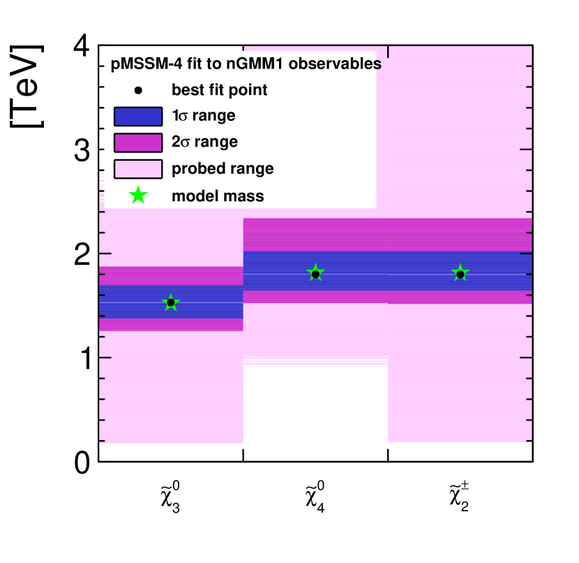
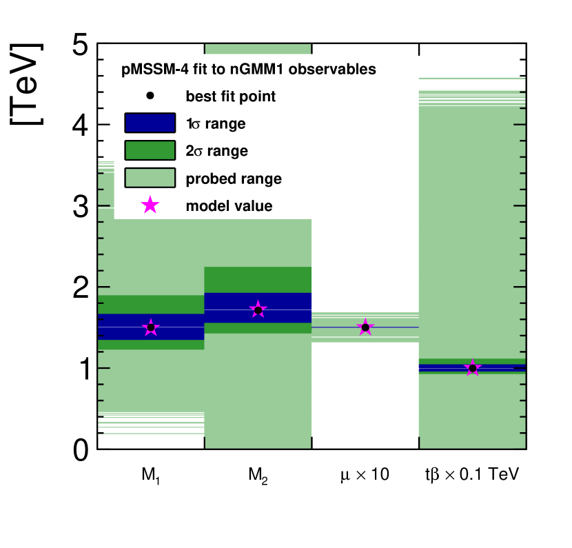
Refer to caption
(a) Fitted masses
Refer to caption
(b) Fitted parameters
Figure 22: Predicted mass and SUSY parameter ranges from the pMSSM-4 fit to nGMM1. The green/magenta star indicates the true model values, while the black dot shows the best fit point.

5.3 Dark Matter in Higgsino Fits

An additional benefit from our fits to MSSM parameters is that it is possible to extract various WIMP dark matter related observables[70]. These include 1. the thermally-produced WIMP relic density Ωχ~TPh2superscriptsubscriptΩ~𝜒TPsuperscript2\Omega_{\tilde{\chi}}^{\rm TP}h^{2}, 2. the spin-dependent (SD) and spin-independent (SI) WIMP-nucleon scattering cross section (e.g. σSI(χp)superscript𝜎SI𝜒𝑝\sigma^{\rm SI}(\chi p)) which is constrained by WIMP direct detection search experiments, and 3. the thermally-averaged WIMP-WIMP annihilation cross-section times relative velocity (evaluated as v0𝑣0v\rightarrow 0) σvdelimited-⟨⟩𝜎𝑣\langle\sigma v\rangle which is constrained by indirect WIMP search results which look for cosmic WIMP-WIMP annihilation to high energy photons and anti-matter. The theory predictions for these observables from IsaReD[73] and IsaReS[74] are listed in Tab. 1. The higgsino-like WIMPs are thermally underproduced as dark matter and if their abundance is augmented via non-thermal WIMP production, then the higgsino-like WIMPs are excluded by direct and indirect WIMP search experiments [71]. However, by requiring naturalness in the QCD sector (i.e. the axionic solution to the strong CP𝐶𝑃CP problem) as well as in the electroweak sector, then we are led to require the presence of axionic dark matter as well. Thus, from naturalness, we expect two dark matter particles: axions as well as higgsino-like WIMPs. In fact, detailed calculations using eight coupled Boltzmann equations (which track axion, WIMP, axino, saxion, gravitino and radiation abundances) suggest that the axions usually dominate the dark matter abundance [72]. Then the diminished presence of higgsinos in the relic DM density leads to consistency with WIMP search results since there are fewer higgsinos present in the relic abundance (typically 10-20%) than is usually assumed (100%).

To obtain these fitted values, we use Fittino [64] together with MicrOmegas [bib:micromegas] and AstroFit [56]. The fitted and scaled relic density is plotted and the 2σ𝜎\sigma confidence interval has been extracted. The centre of the 2σ2𝜎2\sigma confidence level is calculated and used as the mean. The width of the 2σ2𝜎2\sigma range is divided by two to obtain the 1σ𝜎\sigma width assuming the Δχ2Δsuperscript𝜒2\Delta\chi^{2} distribution is parabolic. The distributions are more flat than parabolic so this procedure gives a conservative estimate of the 1σ1𝜎1\sigma width. The relic density distribution from each fit is plotted, assuming a gaussian distribution, in Fig. 23. In case of the pMSSM-10 fit without any further inputs, the relic density is not sufficiently constrained. However this has been traced to be due to fit solutions with extremely low gluino masses of less than 200 GeV. Excluding these points, the blue dashed curves are obtained, which show a very good determination of the relic density agreeing quite well with the theoretical value. The precision improves even further when the pMSSM4 fit is run after the pMSSM10 fit. Such a measurement of the relic density would clearly confirm a possible underabundance of higgsino-like WIMPs.

We also fit the expected values of σSI(χp)superscript𝜎SI𝜒𝑝\sigma^{\rm SI}(\chi p) and σvdelimited-⟨⟩𝜎𝑣\langle\sigma v\rangle which are listed in Tab. 22 (these theory values are somewhat higher than those obtained in Tab. 1 using IsaReS [74] due to Isajet/Spheno spectrum differences and different coding algorithms for direct/indirect detection rates). The σSIsuperscript𝜎SI\sigma^{\rm SI} values can be fit to an accuracy typically better than 1% while the σvdelimited-⟨⟩𝜎𝑣\langle\sigma v\rangle values are typically fit to 10%similar-toabsentpercent10\sim 10\% or worse. By comparing the direct detection rates from WIMP detection experiments to the ILC fitted values for a measured higgsino mass mχsubscript𝑚𝜒m_{\chi}, a direct measurement of WIMP relic density can be made since the WIMP direct detection rates are actually sensitive to ξσSI𝜉superscript𝜎SI\xi\sigma^{\rm SI} where ξ𝜉\xi is the ratio of actual WIMP abundance divided by the total measured abundance Ωa+χh2subscriptΩ𝑎𝜒superscript2\Omega_{a+\chi}h^{2}. Such interplay between ILC results and direct detection results offer direct confirmation that WIMPs would comprise only a portion of dark matter. In addition, indirect WIMP detection rates are proportional to ξ2superscript𝜉2\xi^{2} since they search for WIMP-WIMP annihilation. The interplay of ILC results with indirect WIMP detection rates could offer further confirmation for multicomponent dark matter.
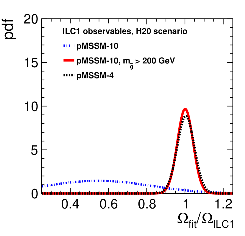
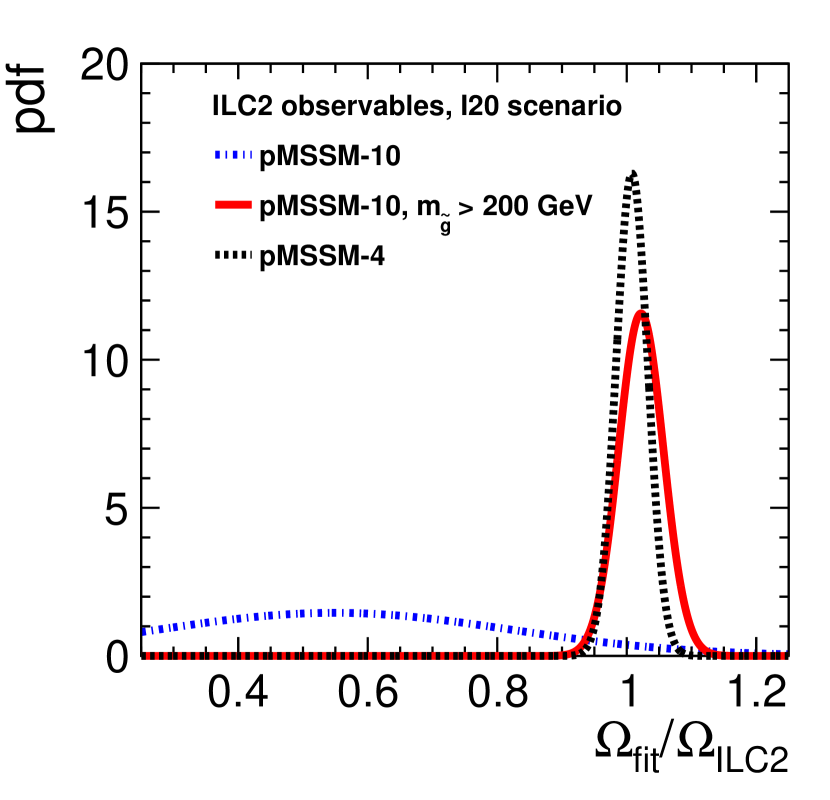
Refer to caption
(a) ILC1
Refer to caption
(b) ILC2
Refer to caption
(c) nGMM1
Figure 23: Fitted relic densities in ILC1, ILC2 and nGMM1 fits.

observableILC1ILC2nGMM1σSI model [109 pb]259.3316.9328.5σSI best fit [109 pb]260.76.9+4.1317.02.1+2.1328.50.9+1.5σv model [1027 cm3s1]15.363.4390.597σv best fit [1027 cm3s1]15.010.88+1.523.5010.523+5.7410.6210.165+0.994missing-subexpressionmissing-subexpressionmissing-subexpressionmissing-subexpressionmissing-subexpressionmissing-subexpressionmissing-subexpressionmissing-subexpressionobservableILC1ILC2nGMM1missing-subexpressionmissing-subexpressionmissing-subexpressionmissing-subexpressionsuperscript𝜎SI model delimited-[]superscript109 pb259.3316.9328.5superscript𝜎SI best fit delimited-[]superscript109 pbsubscriptsuperscript260.74.16.9subscriptsuperscript317.02.12.1subscriptsuperscript328.51.50.9delimited-⟨⟩𝜎𝑣 model delimited-[]superscript1027superscript cm3superscripts115.363.4390.597delimited-⟨⟩𝜎𝑣 best fit delimited-[]superscript1027superscript cm3superscripts1subscriptsuperscript15.011.520.88subscriptsuperscript3.5015.7410.523subscriptsuperscript0.6210.9940.165missing-subexpressionmissing-subexpressionmissing-subexpressionmissing-subexpression\begin{array}[]{ c c c c }\hline\cr\hline\cr\text{observable}&\text{ILC1}&\text{ILC2}&\text{nGMM1}\\ \hline\cr\sigma^{\rm SI}\text{ model }[10^{-9}\text{ pb}]&259.3&316.9&328.5\\ \sigma^{\rm SI}\text{ best fit }[10^{-9}\text{ pb}]&260.7^{+4.1}_{-6.9}&317.0^{+2.1}_{-2.1}&328.5^{+1.5}_{-0.9}\\ \langle\sigma v\rangle\text{ model }[10^{-27}\text{ cm}^{3}\text{s}^{-1}]&15.36&3.439&0.597\\ \langle\sigma v\rangle\text{ best fit }[10^{-27}\text{ cm}^{3}\text{s}^{-1}]&15.01^{+1.52}_{-0.88}&3.501^{+5.741}_{0.523}&0.621^{+0.994}_{-0.165}\\ \hline\cr\hline\cr\end{array}

Table 22: Relic density from MicrOMEGAs and Astrofit, and direct and indirect detection cross sections from Astrofit in the pMSSM-10 fits to ILC1, ILC2 and nGMM1 observables (without the gluino mass measurement). ΩPlancksubscriptΩPlanck\Omega_{\text{Planck}} is taken to be 0.1199 [75].

6 Testing gaugino mass unification

The pMSSM parameters which were extracted in Sec. 5.2 were fitted at the energy scale Q=1𝑄1Q=1 TeV. The scale dependence of the parameters is governed by their renormalization group equations or RGEs. Using the MSSM RGEs, the fitted parameters can be evolved to higher energy scales in order to check hypotheses regarding unification. Specifically, we will test unification of the various gaugino masses which are assumed to unify at Q=mGUT2×1016𝑄subscript𝑚GUTsimilar-to-or-equals2superscript1016Q=m_{\rm GUT}\simeq 2\times 10^{16} GeV (the scale at which gauge couplings unify) in models like NUHM2 and NUHM3 but which would unify at a lower scale in models such as nGMM1. Since in this work we do not subscribe to any particular GUT or string theory, GUT scale threshold corrections to gauge and Yukawa couplings and soft SUSY breaking terms are not imposed.

This section continues the program initiated by Blair et al. of extracting tests of high scale unification from weak scale measurements of SUSY particle properties at ILC[76, 77]. Since the estimates of the achievable precision for the experimental observables used in Sec. 5 are somewhat more pessimistic than the results obtained in Sec. 4, we also discuss the expected impact of the experimental improvements taking the nGMM1 benchmark as an example.

6.1 Method

The running pMSSM-10 weak scale parameters and error bars are extracted using Fittino and SPheno3.3.9beta at Q=1𝑄1Q=1 TeV. Then a random scan of 104superscript10410^{4} samples of the 10 parameters is performed, approximating the parameter PDFs as either Gaussian or flat within ±1σplus-or-minus1𝜎\pm 1\sigma, depending on the shape of their χ2superscript𝜒2\chi^{2} distribution, see e.g. Fig. 19. For each of the sampled points, SPheno was used to calculate the running parameters at each of 21 energy scales between 919191 and 1019superscript101910^{19} GeV. The mean and standard distribution of these parameters’ distributions at each energy scale were used to define confidence bands, as shown in e.g. Fig. 22(b). The unification scale Qunifsubscript𝑄unifQ_{\mathrm{unif}} is determined by fitting linear functions the running parameters in a range close to the visible intersection and extracting the intersection point. With each value for Qunifsubscript𝑄unifQ_{\mathrm{unif}}, a corresponding estimate of M1/2subscript𝑀12M_{1/2} is determined. Gaussian functions can be fitted to the distributions of the resulting values for Qunifsubscript𝑄unifQ_{\mathrm{unif}} and M1/2subscript𝑀12M_{1/2} in order to obtain central values and uncertainties.

For the gluino mass, several scenarios are considered: the determination from loop contributions to the higgsino observables only, a direct observation at the LHC resulting in a precision of 10%percent1010\% on the physical gluino mass, or simply by assuming gaugino mass unification. In the latter case, the extracted mean M1/2subscript𝑀12M_{1/2} and Qunifsubscript𝑄unifQ_{\mathrm{unif}} values can be used to determine the value of M3(Q=1TeV)subscript𝑀3𝑄1TeVM_{3}(Q=1\ {\rm TeV}) and consequently the physical gluino mass. In this case, predictions for the expected value of mg~subscript𝑚~𝑔m_{\tilde{g}} may be made which can serve as a target for future hadron collider searches or compared to the mass of an already-discovered gluino.

6.2 Running gaugino masses for ILC1

The weak scale ILC1 parameters are sampled according to Gaussian distributions for M1subscript𝑀1M_{1} and M2subscript𝑀2M_{2} and uniformly within the 1σ1𝜎1\sigma range for M3subscript𝑀3M_{3}, motivated by the shape of the χ2superscript𝜒2\chi^{2} distributions obtained in the pMSSM-10 fits discussed in Sec. 5.2.1. The resulting running of the gaugino mass parameters in the ILC1 pMSSM-10 fit is plotted in Fig. 24(a). From the plot, it can be seen that M1subscript𝑀1M_{1} and M2subscript𝑀2M_{2} cross near 1016superscript101610^{16} GeV which would verify the prediction of a SUSY GUT model. The uncertainty band for M3subscript𝑀3M_{3} is quite wide but is consistent with the hypothesis of unification of all three gaugino masses at the same energy scale. The extracted unification scale Qunifsubscript𝑄unifQ_{\mathrm{unif}} for M1subscript𝑀1M_{1} and M2subscript𝑀2M_{2} is plotted in Fig. 25(a) from which it can be seen that the distribution follows a Gaussian. The gaugino mass unification scale is found to be Qunif=3.8×10¹⁶subscript𝑄unif3.8superscript1016Q_{\mathrm{unif}}=3.8\times 10^{16} GeV with a 68% confidence range of [3.0×1015,4.9×1017]3.0superscript10154.9superscript1017[3.0\times 10^{15},4.9\times 10^{17}] GeV. From Fig. 25(b), the unified gaugino mass parameter is found to be M1/2=583±40subscript𝑀12plus-or-minus58340M_{1/2}=583\pm 40 GeV in agreement with the GUT scale model model fit.

If it is then assumed that the unification is due to an NUHM2 model, and true model parameter values are assumed for parameters other than M1/2subscript𝑀12M_{1/2}, then instead M3subscript𝑀3M_{3} can be extracted by running down in energy to find the running value of M3(Q=1TeV)subscript𝑀3𝑄1TeVM_{3}(Q=1\ {\rm TeV}). From Fig. 24(b) we obtain M3(Q=1TeV)=1216±76subscript𝑀3𝑄1TeVplus-or-minus121676M_{3}(Q=1\ {\rm TeV})=1216\pm 76 GeV (which agrees with the the weak scale fitted value). Consequently, a prediction for the physical gluino mass can be obtained: mg~=1467±80subscript𝑚~𝑔plus-or-minus146780m_{\tilde{g}}=1467\pm 80 GeV which could then be checked against results from hadron collider searches.
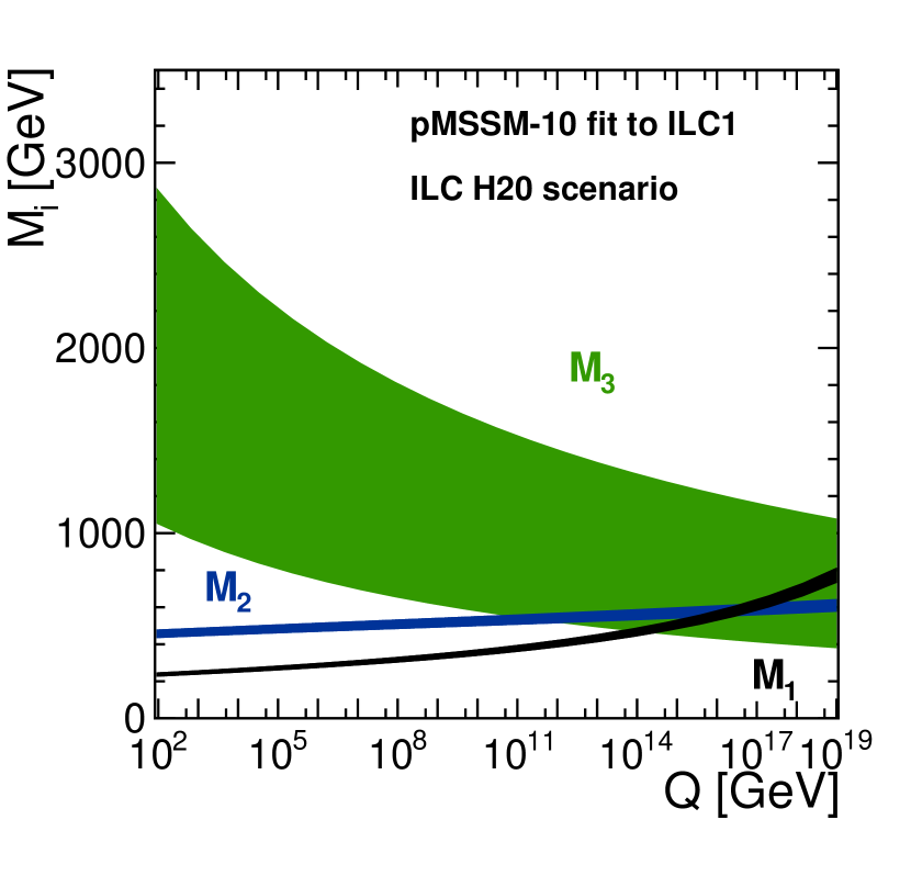
Refer to caption
(a)
Refer to caption
(b)
Figure 24: The running gaugino masses Misubscript𝑀𝑖M_{i} based on the pMSSM-10 fit to ILC1 observables. The bands correspond to one standard deviation. (a) Using M3subscript𝑀3M_{3} at the weak scale as constrained from ILC measurements (b) M3subscript𝑀3M_{3} is assumed to unify with M1subscript𝑀1M_{1} and M2subscript𝑀2M_{2} and then run to the weak scale to gain a prediction for M3subscript𝑀3M_{3}(Q=1𝑄1Q=1 TeV).
Refer to caption
(a) Unification scale Qunifsubscript𝑄unifQ_{\mathrm{unif}}
Refer to caption
(b) unified gaugino mass M1/2subscript𝑀12M_{1/2}
Figure 25: Distribution of the unification scale Qunifsubscript𝑄unifQ_{\mathrm{unif}} and unified gaugino mass M1/2subscript𝑀12M_{1/2} obtained from the running parameters M1subscript𝑀1M_{1} and M2subscript𝑀2M_{2} and their uncertainties from the pMSSM-10 fit to ILC1 observables.

6.3 Running gaugino masses for ILC2

The uncertainties of the weak scale gaugino mass fit parameters are larger in the case of ILC2 as compared to ILC1. Still, the weak scale ILC2 parameters are sampled according to Gaussian distributions for M1subscript𝑀1M_{1} and M2subscript𝑀2M_{2} and uniformly within the 1σ1𝜎1\,\sigma range for M3subscript𝑀3M_{3}, motivated by the shape of the χ2superscript𝜒2\chi^{2} distributions obtained in the pMSSM-10 fits discussed in Sec. 5.2.2. The larger uncertainties are reflected in the running gaugino mass plots in Fig. 26(a) and 26(b). Nevertheless, it is still possible to verify that M1subscript𝑀1M_{1} and M2subscript𝑀2M_{2} unify near the GUT scale. For ILC2, the fitted weak scale error band for M3subscript𝑀3M_{3} is so wide that it is consistent with unification with M1subscript𝑀1M_{1} or M2subscript𝑀2M_{2} at almost any scale.

Refer to caption
(a)
Refer to caption
(b)
Figure 26: The running gaugino masses Misubscript𝑀𝑖M_{i} based on the pMSSM-10 fit to ILC2 observables. The bands correspond to one standard deviation. (a) Using M3subscript𝑀3M_{3} at the weak scale as constrained from ILC measurements (b) M3subscript𝑀3M_{3} is assumed to unify with M1subscript𝑀1M_{1} and M2subscript𝑀2M_{2} and then run to the weak scale to gain a prediction for M3subscript𝑀3M_{3}(Q=1𝑄1Q=1 TeV).
Refer to caption
(a) Unification scale Qunifsubscript𝑄unifQ_{\mathrm{unif}}
Refer to caption
(b) unified gaugino mass M1/2subscript𝑀12M_{1/2}
Figure 27: Distribution of the unification scale Qunifsubscript𝑄unifQ_{\mathrm{unif}} and unified gaugino mass M1/2subscript𝑀12M_{1/2} obtained from the running parameters M1subscript𝑀1M_{1} and M2subscript𝑀2M_{2} and their uncertainties from the pMSSM-10 fit to ILC2 observables.

Using the same methodology as for ILC1, the unification scale for ILC2 where M1=M2subscript𝑀1subscript𝑀2M_{1}=M_{2} is found to be Gaussian with a mean of Qunif=1.5×10¹⁶subscript𝑄unif1.5superscript1016Q_{\mathrm{unif}}=1.5\times 10^{16} GeV with a 68% confidence interval of [5.4×1013,4.4×1018]5.4superscript10134.4superscript1018[5.4\times 10^{13},4.4\times 10^{18}] GeV, as shown in Fig. 27(a). The unified value of M1/2subscript𝑀12M_{1/2} is found in Fig. 27(b) to be Gaussian with M1/2=1220±170subscript𝑀12plus-or-minus1220170M_{1/2}=1220\pm 170 GeV which corresponds to the GUT scale fit model value. If M3subscript𝑀3M_{3} is instead assumed to unify with M1subscript𝑀1M_{1} and M2subscript𝑀2M_{2} at Qunifsubscript𝑄unifQ_{\mathrm{unif}} and the NUHM2 model is adopted, then the extrapolated value of M3subscript𝑀3M_{3} at 111 TeV is found to be M3(Q=1TeV)=2616±582subscript𝑀3𝑄1TeVplus-or-minus2616582M_{3}(Q=1\ {\rm TeV})=2616\pm 582 GeV while the physical gluino mass is found to be mg~=2872±605subscript𝑚~𝑔plus-or-minus2872605m_{\tilde{g}}=2872\pm 605 GeV. Such a large value may serve as a target for gluino pair searches at upgraded hadron colliders.

6.4 Running gaugino masses for nGMM1

The running of the gaugino mass parameters in the nGMM1 benchmark model differs from the running in the ILC1 and ILC2 models. There are two reasons: 1. the underlying model is now a mirage unification model where the gaugino mass parameters unify at an intermediate energy scale and 2. the determination of M1subscript𝑀1M_{1} and M2subscript𝑀2M_{2} from the weak scale fits is much less accurate in nGMM1 as compared to the ILC1 and ILC2 benchmark models.

Figure 28(a) shows the running gaugino masses resultant from the pMSSM-10 fit with absolute masses as input as described in Sec. 5.2.3. Even in this most conservative case, the plot is certainly inconsistent with any sort of GUT scale unification of gaugino masses. From a closer look we notice that the hierarchy between M1subscript𝑀1M_{1} and M2subscript𝑀2M_{2} at Q=1𝑄1Q=1 TeV is not well defined, and that actually the M1subscript𝑀1M_{1} band seems to start above the lower rim of the M2subscript𝑀2M_{2} band. This effect occurs since, motivated by the shape of the χ2superscript𝜒2\chi^{2} landscape of the pMSSM-10 fit (c.f. Fig. 19), M1subscript𝑀1M_{1} and M3subscript𝑀3M_{3} are sampled from a uniform distribution and only M2subscript𝑀2M_{2} is treated with a Gaussian. In addition the 1σ1𝜎1\,\sigma interval for M1subscript𝑀1M_{1} is very asymmetric around the best fit point (c.f. Tab. 20). In combination with the flat sampling, the 1σ1𝜎1\,\sigma band for M1subscript𝑀1M_{1} seems to start much higher than the best fit value for M1subscript𝑀1M_{1} would indicate.

Refer to caption
(a)
Refer to caption
(b)
Figure 28: The running of the gaugino masses after extracting their weak scale values from a fit to nGMM1 observables. The bands correspond to one standard deviation. (a) pMSSM-10 fit result with absolute masses as input from Sec. 5.2.3 (b) estimated effect of improvement from using the full simulation results from Sec. 4.3, and from including a 10% measurement of the gluino mass from HL-LHC (or other future hadron collider). In addition a fit of the pMSSM-4 parameters, and M3subscript𝑀3M_{3} as a fit parameter, is run, as discussed at the beginning of Sec. 5.2. The Markov chain had a length of 105superscript10510^{5} points.

A substantial improvement of the precision can be seen in Fig. 28(b), which shows the analogous result obtained when using the improved experimental precisions presented in Sec. 4.3 plus a 10% measurement of the gluino mass from the HL-LHC (or other future hadron collider). In addition to the improved inputs, the parameter extraction has also been refined: the estimates of M1subscript𝑀1M_{1}, M2subscript𝑀2M_{2} and M3subscript𝑀3M_{3} at the weak scale are obtained from a fit of only the pMSSM-4 parameters and M3subscript𝑀3M_{3}, which could be run subsequently to an initial pMSSM-10 fit as outlined at the beginning of Sec. 5.2. In this case, all parameters can be sampled from Gaussian distributions, as can be seen from Fig. 19. The weak scale hierarchy between M1subscript𝑀1M_{1} and M2subscript𝑀2M_{2} is now well determined, and a clear crossing of all three bands is found at a scale much lower than the GUT scale: around 107108superscript107superscript10810^{7}-10^{8} GeV, consistent with the theory mass unification scale for the model point which occurs at 107superscript10710^{7} GeV.

This is not even the most optimistic case, since further improvements can be expected from using the higgsino mass differences instead as input (c.f. Fig. 21(d)) and from more precise χ~1±superscriptsubscript~𝜒1plus-or-minus\widetilde{\chi}_{1}^{\pm} and χ~20superscriptsubscript~𝜒20\widetilde{\chi}_{2}^{0} masses extracted from scanning the thresholds of χ~1+superscriptsubscript~𝜒1\widetilde{\chi}_{1}^{+}χ~1superscriptsubscript~𝜒1\widetilde{\chi}_{1}^{-} and χ~20superscriptsubscript~𝜒20\widetilde{\chi}_{2}^{0}χ~i0superscriptsubscript~𝜒𝑖0\widetilde{\chi}_{i}^{0} production, respectively. In addition, the consideration of further constraints from improved EWPOs, flavour physics, direct search limits etc. is expected to further improve the weak scale parameter determination.
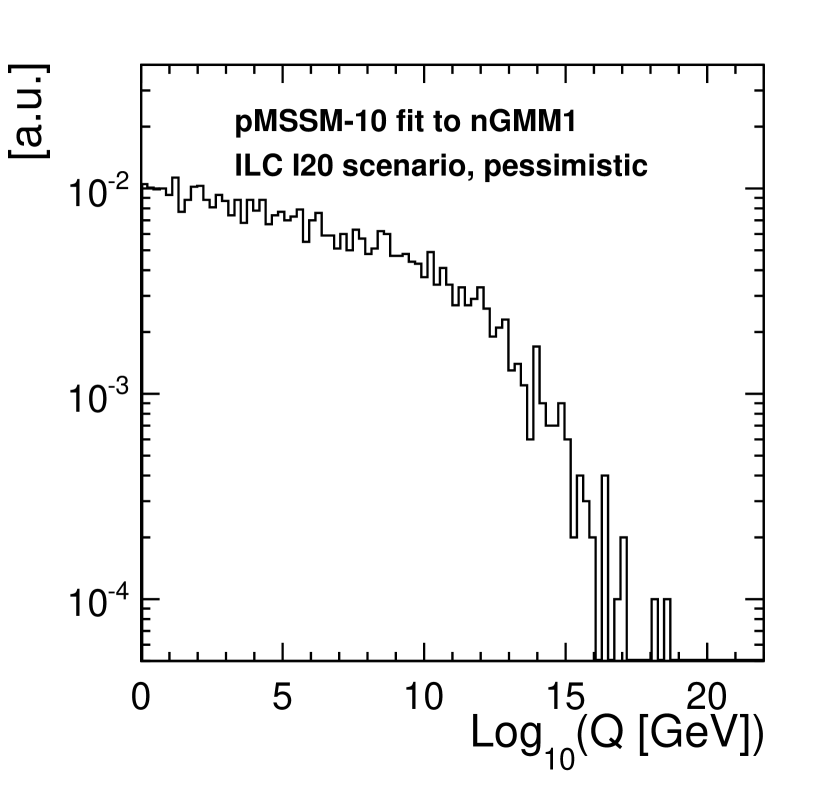
Refer to caption
(a) Unification scale Qunifsubscript𝑄unifQ_{\mathrm{unif}}
Refer to caption
(b) unified gaugino mass M1/2subscript𝑀12M_{1/2}
Figure 29: Distribution of the unification scale Qunifsubscript𝑄unifQ_{\mathrm{unif}} and unified gaugino mass M1/2subscript𝑀12M_{1/2} obtained from the running parameters M1subscript𝑀1M_{1} and M2subscript𝑀2M_{2} and their uncertainties from the pMSSM-10 fit to nGMM1 observables.

For the conservative version of the running masses in Fig. 28(a), we quantify the constraints on the unification scale in Fig. 29a. While the distribution of obtained Qunifsubscript𝑄unifQ_{\mathrm{unif}} values has no clear peak, it increases towards lower unification scales, away from the GUT scale. A unification at 1016similar-toabsentsuperscript1016\sim 10^{16} GeV is excluded with 99.9% probability. The most probable unified value of M1/2subscript𝑀12M_{1/2} was found to be 1600±450plus-or-minus16004501600\pm 450 GeV in Fig. 29b. The drastic improvement in Fig. 28(b) compared to Fig. 28, illustrates the substantial impact which can be expected from further refinements of the underlying analysis.

Due to the extracted gaugino mass unification scale not matching with the GUT scale, there would be important implications for SUSY model building. It is noteworthy that the pMSSM fit and the fit parameter evolution indicate that the underlying model does not have gaugino mass unification, even though the fit of NUHM2 parameters to the nGMM1 observables presented in Sec. 5.1 does not entirely rule NUHM2 out as a possible model.

7 Summary and conclusions

Supersymmetry with radiatively-driven naturalness is especially compelling in that it reconciles electroweak naturalness with (multi-TeV) LHC sparticle mass limits and Higgs boson mass measurements. The most fundamental consequence of radiatively-driven natural SUSY is the prediction of four light higgsinos χ1±superscriptsubscript𝜒1plus-or-minus\chi_{1}^{\pm}, χ1,20superscriptsubscript𝜒120\chi_{1,2}^{0} with mass 100300similar-toabsent100300\sim 100-300 GeV (the lower the better). Such light higgsinos are difficult (but perhaps not impossible) to see at LHC, but would be easily visible at ILC operating with s>2m(higgsino)𝑠2𝑚𝑖𝑔𝑔𝑠𝑖𝑛𝑜\sqrt{s}>2m(higgsino). In this case, the ILC, initially constructed as a Higgs factory, would turn out to be a higgsino factory! Thus, for this highly motivated scenario, ILC could serve as both a SUSY discovery (or confirmation) machine, and a precision microscope.

In this paper we have examined the capability of experiments at the ILC to both discover (or confirm) supersymmetry and to make precision measurements of superparticle properties that would probe the superpotential higgsino mass parameter μ𝜇\mu via direct sparticle mass measurements and in addition provide a measurement of SUSY-breaking gaugino mass parameters via the higgsino mass splittings.

When these measurements are combined with precision Higgs boson measurements, precision fits to both weak scale SUSY and high scale SUSY model parameters can be made. We have investigated the capability of ILC to discover light higgsinos in three natural SUSY benchmark models: two with unified gaugino masses and one with mirage unification of gaugino masses at an intermediate mass scale between mGUTsubscript𝑚GUTm_{\rm GUT} and mweaksubscript𝑚𝑤𝑒𝑎𝑘m_{weak}. Our calculations implement a detailed ILD detector simulation along with event generation from Whizard.

By measuring e+eχ~1+χ~1(νχ~10)+(qq¯χ~10)superscript𝑒superscript𝑒superscriptsubscript~𝜒1superscriptsubscript~𝜒1subscript𝜈superscriptsubscript~𝜒10𝑞superscript¯𝑞superscriptsubscript~𝜒10e^{+}e^{-}\rightarrow\tilde{\chi}_{1}^{+}\tilde{\chi}_{1}^{-}\rightarrow(\ell\nu_{\ell}\tilde{\chi}_{1}^{0})+(q\bar{q}^{\prime}\tilde{\chi}_{1}^{0}) we are able to extract mχ~1±subscript𝑚superscriptsubscript~𝜒1plus-or-minusm_{\tilde{\chi}_{1}^{\pm}} and mχ~10subscript𝑚superscriptsubscript~𝜒10m_{\tilde{\chi}_{1}^{0}} via the m(jj)𝑚𝑗𝑗m(jj) and E(jj)𝐸𝑗𝑗E(jj) distributions, typically to percent level accuracy. By measuring the dilepton mass and energy distributions from e+eχ~20χ~10superscript𝑒superscript𝑒superscriptsubscript~𝜒20superscriptsubscript~𝜒10e^{+}e^{-}\rightarrow\tilde{\chi}_{2}^{0}\tilde{\chi}_{1}^{0} followed by χ~20+χ~10superscriptsubscript~𝜒20superscriptsuperscriptsuperscriptsubscript~𝜒10\tilde{\chi}_{2}^{0}\rightarrow\ell^{+}\ell^{-}\tilde{\chi}_{1}^{0}, we are able to measure mχ~10subscript𝑚superscriptsubscript~𝜒10m_{\tilde{\chi}_{1}^{0}} and mχ~20subscript𝑚superscriptsubscript~𝜒20m_{\tilde{\chi}_{2}^{0}} to typically percent level accuracy. We combine the higgsino mass measurements with precision higgsino pair production cross section measurements using different beam polarizations.

When these precision higgsino measurements are combined with precision Higgs boson measurements, precision fits to both weak scale SUSY and high scale SUSY model parameters can be made. In particular, an indirect measurement of wino and bino SUSY breaking masses can be extracted from the higgsino mass splittings. When extrapolated to high energies, the hypothesis of gaugino mass unification can be tested. If combined with LHC gluino mass measurements, the unification of all three gaugino masses may be explored. Such measurements will shed light on different possibilities for SUSY breaking as may be expected in SUSY GUT models or in models with mixed moduli- and anomaly- (mirage) mediation. In addition, fits of SUSY dark matter observables may shed light on the nature of dark matter, such as confirming or ruling out multi-component dark matter as expected from natural SUSY where both higgsino-like WIMPs and axions are expected to be produced in the early universe.

Thus, in assessing the ILC capabilities in this compelling SUSY extension of the SM, we conclude that ILC can indeed serve as a SUSY discovery machine and precision microscope, offering a window into the intricacies of SUSY breaking and fundamental particle physics and providing insights into the nature of dark matter and cosmology.

8 Acknowledgments

This work was supported in part by the Office of Science, US Department of Energy and by the Deutsche Forschungsgemeinschaft (DFG) through the Collaborative Research Centre SFB 676 “Particles, Strings and the Early Universe”, project B1. We would like to thank the LCC generator working group and the ILD software working group for providing the simulation and reconstruction tools and producing the Monte Carlo samples used in this study. This work has benefited from computing services provided by the ILC Virtual Organization, supported by the national resource providers of the EGI Federation and the Open Science GRID, and of those of the German National Analysis Facility (NAF).

Appendix A Additional Figures and Tables

.

Table 23: Expected number of events for chargino signal and major backgrounds for the electron final state and beam polarization 𝒫+subscript𝒫absent\mathcal{P}_{-+}. The integrated luminosity is assumed to be 500 fb-1. For each benchmark model, the background refers to the other SUSY backgrounds.
χ~1+χ~1χ~10χ~10qq¯eνesubscriptsuperscript~𝜒1subscriptsuperscript~𝜒1subscriptsuperscript~𝜒01subscriptsuperscript~𝜒01𝑞superscript¯𝑞𝑒subscript𝜈𝑒\widetilde{\chi}^{+}_{1}\widetilde{\chi}^{-}_{1}\rightarrow\widetilde{\chi}^{0}_{1}\widetilde{\chi}^{0}_{1}q\bar{q}^{\prime}e\nu_{e} ILC1 ILC2 nGMM1 SM bkg.
500 GeV, 500 fb-1, 𝒫+subscript𝒫absent\mathcal{P}_{-+} Signal Bkg. Signal Bkg. Signal Bkg. e+esuperscript𝑒superscript𝑒absente^{+}e^{-}\rightarrow2f e+esuperscript𝑒superscript𝑒absente^{+}e^{-}\rightarrow4f γγ𝛾𝛾absent\gamma\gamma\rightarrow 2f eγ𝑒𝛾absente\gamma\rightarrow3f γγ𝛾𝛾absent\gamma\gamma\rightarrow4f
Preselection 53963 423992 41962 322011 66118 476646 11906936 14941264 307189572 65344394 61765
Lepton selection 4926 11922 2733 7676 4453 12325 543911 914027 93465142 21607557 1905
BeamCal veto 4869 11752 2707 7602 4414 12188 495890 748137 1284355 3964924 1772
pT>5subscript𝑝𝑇5p_{T}>5 GeV 3146 2323 1242 1110 1337 1109 226624 506571 967020 3804929 1328
Ntrk,jet2subscript𝑁trkjet2N_{\rm trk,jet}\geq 2 2285 324 667 108 515 98 42892 220378 65284 1745715 627
|cosθj|<0.98subscript𝜃𝑗0.98|\cos\theta_{j}|<0.98 2225 314 652 106 504 97 15612 168407 50786 1323463 513
Δϕ<1.0Δitalic-ϕ1.0\Delta\phi<1.0 1544 122 411 30 296 19 1507 34570 11157 533787 51
|cosθjj|<0.2subscript𝜃𝑗𝑗0.2|\cos\theta_{jj}|<0.2 1535 90 405 24 293 17 1360 32195 9471 483002 40
Evis<80subscript𝐸vis80E_{\rm vis}<80 1496 87 402 24 291 17 59 403 1810 7835 2.9
Emiss>400subscript𝐸miss400E_{\rm miss}>400 1485 87 402 24 291 17 12 69 7.1 48 2.0
|cosθmiss|<0.99subscript𝜃miss0.99|\cos\theta_{\rm miss}|<0.99 1463 85 392 23 283 15 5.9 64 0.0 22 2.0
Table 24: Expected number of events for chargino signal and major backgrounds for the muon final state and beam polarization 𝒫+subscript𝒫absent\mathcal{P}_{-+}. The integrated luminosity is assumed to be 500 fb-1. For each benchmark model, the background refers to the other SUSY backgrounds.
χ~1+χ~1χ~10χ~10qq¯μνμsubscriptsuperscript~𝜒1subscriptsuperscript~𝜒1subscriptsuperscript~𝜒01subscriptsuperscript~𝜒01𝑞superscript¯𝑞𝜇subscript𝜈𝜇\widetilde{\chi}^{+}_{1}\widetilde{\chi}^{-}_{1}\rightarrow\widetilde{\chi}^{0}_{1}\widetilde{\chi}^{0}_{1}q\bar{q}^{\prime}\mu\nu_{\mu} ILC1 ILC2 nGMM1 SM bkg.
500 GeV, 500 fb-1, 𝒫+subscript𝒫absent\mathcal{P}_{-+} Signal Bkg. Signal Bkg. Signal Bkg. e+esuperscript𝑒superscript𝑒absente^{+}e^{-}\rightarrow2f e+esuperscript𝑒superscript𝑒absente^{+}e^{-}\rightarrow4f γγ𝛾𝛾absent\gamma\gamma\rightarrow 2f eγ𝑒𝛾absente\gamma\rightarrow3f γγ𝛾𝛾absent\gamma\gamma\rightarrow4f
Preselection 53459 424497 41714 322259 65104 477660 11906936 14941264 307189572 65344394 61765
Lepton selection 5748 32945 3497 21394 6194 34867 1125893 1297965 42676970 2497567 2716
BeamCal veto 5683 32500 3462 21165 6134 34476 1025945 1049378 420779 325406 2475
pT>5subscript𝑝𝑇5p_{T}>5 GeV 3677 3141 1566 1720 1832 1794 99197 345356 101920 146861 1430
Ntrk,jet2subscript𝑁trkjet2N_{\rm trk,jet}\geq 2 2612 710 805 225 690 228 19319 183151 197 10945 509
|cosθj|<0.98subscript𝜃𝑗0.98|\cos\theta_{j}|<0.98 2544 688 784 221 672 223 11089 150507 28 7906 331
Δϕ<1.0Δitalic-ϕ1.0\Delta\phi<1.0 1972 259 532 53 412 40 755 37957 28 874 55
|cosθjj|<0.2subscript𝜃𝑗𝑗0.2|\cos\theta_{jj}|<0.2 1954 118 526 29 406 32 471 37320 0.0 174 51
Evis<80subscript𝐸vis80E_{\rm vis}<80 1905 110 523 28 404 31 59 379 0.0 0.0 22
Emiss>400subscript𝐸miss400E_{\rm miss}>400 1889 110 523 28 404 31 33 39 0.0 0.0 8.0
|cosθmiss|<0.99subscript𝜃miss0.99|\cos\theta_{\rm miss}|<0.99 1862 108 509 28 389 29 33 37 0.0 0.0 7.0

G. Degrassi, S. Heinemeyer, W. Hollik, P. Slavich and G. Weiglein, Eur. Phys. J. C 28 (2003) 133 [hep-ph/0212020]. S. Heinemeyer, W. Hollik and G. Weiglein, Eur. Phys. J. C 9 (1999) 343 [hep-ph/9812472]. S. Heinemeyer, W. Hollik and G. Weiglein, Comput. Phys. Commun.  124 (2000) 76 [hep-ph/9812320].

  • [54] S. Caiazza, “The GridGEMmodule𝐺𝑟𝑖𝑑𝐺𝐸𝑀𝑚𝑜𝑑𝑢𝑙𝑒GridGEMmodule for the ILD TPC and A new algorithm for kinematic edge determination,” PhD Thesis, Universität Hamburg, 2018, doi:10.3204/PUBDB-2018-05289
  • [55] W. Porod, Comput. Phys. Commun.  153, 275 (2003) [arXiv:hep-ph/0301101].
  • [56] N. Nguyen, D. Horns and T. Bringmann, “AstroFit: An Interface Program for Exploring Complementarity in Dark Matter Research,” doi:10.1142/9789814405072_0154 arXiv:1202.1385 [astro-ph.HE].
  • [57] CMS Collaboration [CMS Collaboration], CMS-PAS-HIG-15-004.
  • [58] M. Aaboud et al. [ATLAS Collaboration], Phys. Lett. B 759 (2016) 555 doi:10.1016/j.physletb.2016.06.017 [arXiv:1603.09203 [hep-ex]].
  • [59] M. Aaboud et al. [ATLAS Collaboration], Eur. Phys. J. C 76 (2016) no.11, 585 doi:10.1140/epjc/s10052-016-4400-6 [arXiv:1608.00890 [hep-ex]].
  • [60] The ATLAS collaboration [ATLAS Collaboration], ATLAS-CONF-2017-021.
  • [61] The ATLAS collaboration [ATLAS Collaboration], ATLAS-CONF-2017-037.
  • [62] K. Seidel, F. Simon, M. Tesar and S. Poss, Eur. Phys. J. C 73 (2013) no.8, 2530 doi:10.1140/epjc/s10052-013-2530-7 [arXiv:1303.3758 [hep-ex]].
  • [63] M. Berggren, F. Brümmer, J. List, G. Moortgat-Pick, T. Robens, K. Rolbiecki and H. Sert, Eur. Phys. J. C 73 (2013) no.12, 2660 doi:10.1140/epjc/s10052-013-2660-y [arXiv:1307.3566 [hep-ph]].
  • [64] P. Bechtle, K. Desch and P. Wienemann, Comput. Phys. Commun.  174 (2006) 47 doi:10.1016/j.cpc.2005.09.002 [hep-ph/0412012].
  • [65] H. Baer, A. Mustafayev, S. Profumo, A. Belyaev and X. Tata, Phys. Rev. D 71 (2005) 095008 doi:10.1103/PhysRevD.71.095008 [hep-ph/0412059].
  • [66] S.-L. Lehtinen, “Supersymmetry parameter determination at the International Linear Collider,” PhD Thesis, Hamburg University, 2018.
  • [67] K. Fujii et al., “Physics Case for the International Linear Collider,” arXiv:1506.05992 [hep-ex].
  • [68] T. Barklow, J. Brau, K. Fujii, J. Gao, J. List, N. Walker and K. Yokoya, “ILC Operating Scenarios,” arXiv:1506.07830 [hep-ex].
  • [69] J. Yan, S. Watanuki, K. Fujii, A. Ishikawa, D. Jeans, J. Strube, J. Tian and H. Yamamoto, Phys. Rev. D 94 (2016) no.11, 113002 doi:10.1103/PhysRevD.94.113002 [arXiv:1604.07524 [hep-ex]].
  • [70] E. A. Baltz, M. Battaglia, M. E. Peskin and T. Wizansky, Phys. Rev. D 74 (2006) 103521 doi:10.1103/PhysRevD.74.103521 [hep-ph/0602187].
  • [71] H. Baer, V. Barger, D. Sengupta and X. Tata, Eur. Phys. J. C 78 (2018) no.10, 838 doi:10.1140/epjc/s10052-018-6306-y [arXiv:1803.11210 [hep-ph]].
  • [72] K. J. Bae, H. Baer, A. Lessa and H. Serce, JCAP 1410 (2014) no.10, 082 doi:10.1088/1475-7516/2014/10/082 [arXiv:1406.4138 [hep-ph]].
  • [73] H. Baer, C. Balazs and A. Belyaev, JHEP 0203 (2002) 042.
  • [74] H. Baer, A. Belyaev, T. Krupovnickas and J. O’Farrill, JCAP 0408 (2004) 005 doi:10.1088/1475-7516/2004/08/005 [hep-ph/0405210].
  • [75] P. A. R. Ade et al. [Planck Collaboration], Astron. Astrophys.  594 (2016) A13 doi:10.1051/0004-6361/201525830 [arXiv:1502.01589 [astro-ph.CO]].
  • [76] G. A. Blair, W. Porod and P. M. Zerwas, Phys. Rev. D 63 (2001) 017703 doi:10.1103/PhysRevD.63.017703 [hep-ph/0007107].
  • [77] G. A. Blair, W. Porod and P. M. Zerwas, Eur. Phys. J. C 27 (2003) 263 doi:10.1140/epjc/s2002-01117-y [hep-ph/0210058].
  • [78] P. Bambade et al., “The International Linear Collider: A Global Project,” arXiv:1903.01629 [hep-ex].
  • Conversion to HTML had a Fatal error and exited abruptly. This document may be truncated or damaged.