Double field inflation of generalized dilaton-axion models with a new Fayet-Iliopoulos (FI) term

MAN Ping Kwan, Ellgan^a)†

${Department\;of\;Pure\;and\;Applied\;Physics,\;Waseda\;University}^{\rm a)}$

1 Abstract

We study the inflation dynamics of generalized dilaton-axion models with a new Fayet-Iliopoulos (FI) term. In particular, we find the relationships between the super-potential parameters and the coefficient of natural logarithm of the real part of dilaton-axion fields stored in the Kähler potential based on the vacuum conditions at the end of inflation. We also evaluate the feasible initial field values, their corresponding SUSY breaking scales and the iso-curvature parameters.

2 Introduction

Slow-roll parameters	Range(s)	Spectral indices	Range(s)
${\epsilon}_{V}$	$<0.004$	${n}_{s}-1$	$[-0.0423,-0.0327]$
${\eta}_{V}$	$[-0.021,-0.008]$	$\frac{d{n}_{s}}{d\ln{k}}$	$[-0.008,0.012]$
${\xi}_{V}$	$[-0.0045,0.0096]$	$\frac{d^{2}{n}_{s}}{d\ln{k}^{2}}$	$[-0.003,0.023]$
${H}_{\text{hc}}$	$<2.7\times{10}^{-5}{M}_{\text{pl}}$	${V}_{\text{hc}}$	$<\left(1.7\times{10}^{16}\;\text{GeV}\right)^{4}$

Table 1: Slow roll potential parameters and spectral indices in Planck 2018

Inflation is the vital part for studying the birth of our universe and verifying the consistency of the theory of quantum gravity [Phys.Rev.D23(1981), 347-356, Phys.Lett.91B(1980), 99-102, Mon.Not.Roy.Astron.Soc.195(1981), 467-479]. The latest observation data are shown in Table 1 [5], which are consistent with the slow roll approximation. There are many models satisfying the observation [4, 5], one of which is the most promising model - Starobinsky model (also called $R^{2}$ inflation model), which can be motivated by, for example, modified gravity theory [Phys.Lett.91B(1980), 99-102, 4, 10, 11, 12, 13, 14] and supergravity theory (SUGRA) [15, 16, 17, 18]. Since SUGRA describes high energy physics beyond the Standard model (SM), gravity beyond the $\Lambda$CDM cosmological model and the low energy effective theory of superstring theory, it has been adopted to study the primordial dynamics of the universe evolution. In particular, the extension of Starobinsky model in the new-minimal formulation of SUGRA is dual to the standard counterpart coupled to a massive vector multiplet, or a massless vector multiplet and a Stückelberg chiral multiplet with the Kähler potential in the following form [19, 20, 21]

$$\frac{K\left(T,\bar{T}\right)}{{M}_{\text{pl}}^{2}}=-{\rho}\ln{\left(\frac{T+\bar{T}}{{M}_{\text{pl}}}\right)}+\tilde{\beta}\left(\frac{T+\bar{T}}{{M}_{\text{pl}}}\right),\\$$ (1)

where the last term is the FI term of the gauged $R$-symmetry and spontaneous SUSY breaking occurred after the inflation. [21] showed that this model can be consistent with observations only for ${\rho}=1,2$ with some non-perturbative corrections and SUSY is spontaneously broken at the dS vacuum with gravitino mass in the TeV range. Furthermore, [24] finds that an alternative non-vanishing FI terms [22, 23] can allow inflationary models having the following forms of Kähler potential $K$

$$\frac{K\left(T,\bar{T}\right)}{{M}_{\text{pl}}^{2}}=-{\rho}\ln{\left(\frac{T+\overline{T}}{{M}_{\text{pl}}}\right)}.\\$$ (2)

This Kähler potential model generalizes various models such as no-scale SUGRA [PhenomenologicalSU(1, 1)supergravity, 26, 27, 28, 29, 30, 31] and M theory compactification on a ${G}_{2}$ manifold [32, 33, 34]. The model studied in [24] describes the inflation from the real part of dilaton-axion chiral superfield $T$ with a fixed imaginary part at the dS vacuum. Thus, it is interesting to see how the inflation dynamics changes when the imaginary part also evolves to contribute to the inflation dynamics. That is the main theme of this paper.

In this paper, we are going to study the inflation dynamics of generalized dilaton-axion models, where both the dilaton and its axionic partner simultaneously contribute to the evolution of inflation. The organization of this paper is as follows. In section 3, we give the total potential consisting of $F$ term from the Kähler potential given by Eq.(2) and the Polonyi type super-potential, and $D$ term potential from an alternative FI term [22, 23]. We give the derivatives of the total potential, the possible ranges of parameters under the constraints of dS vacuum and the corresponding SUSY breaking scales in section 4. We summarize our results of dS vacuum in section 5 and the equations of motion (E.O.M.s) of the evolution of dilaton and axion. In section 6, we give the initial conditions and parameters feasible for inflation based on the constraints of Planck observation listed in Table 1 and e-folding number $50$ to $60$. We discuss our results in section 7 and draw conclusions in section 8.

3 General model

Recall the $F$ term potential in $\mathcal{N}=1$ supergravity (SUGRA) is

$${V}_{F}={e}^{\frac{K}{{M}^{2}_{\text{pl}}}}\left({K}^{I\bar{J}}{D}_{I}W{D}_{\bar{J}}\bar{W}-\frac{3}{{M}^{2}_{\text{pl}}}|W|^{2}\right).\\$$ (3)

where

$${K}_{I\bar{J}}\equiv\frac{{\partial}^{2}K}{{\partial}{\Phi}^{I}{\partial}\bar{{\Phi}}^{\bar{J}}},\quad{D}_{I}W\equiv{\partial}_{I}W+\frac{1}{{M}^{2}_{\text{pl}}}\left({\partial}_{I}K\right)W=\frac{{\partial}W}{{\partial}{\Phi}^{I}}+\frac{1}{{M}^{2}_{\text{pl}}}\frac{{\partial}K}{{\partial}{\Phi}^{I}}W,\\$$ (4)

${\Phi}^{I}$ is complex scalar field for all $I$ from $1$ to the dimension of the field space, the upper bar means the complex conjugate of the corresponding variables/ fields, ${K}^{I\bar{J}}$ is the inverse of the Kähler metric ${K}_{I\bar{J}}$ and ${M}_{\text{pl}}$ is the (reduced) Planck mass. Note that the Kähler potential is given by

$$\frac{K\left(T,\bar{T}\right)}{{M}^{2}_{\text{pl}}}=-{\rho}\ln{\left(\frac{T+\bar{T}}{{M}_{\text{pl}}}\right)},\\$$ (5)

while the super-potential is given by

$$W\left(T\right)={\lambda}+{\mu}T,\\$$ (6)

where ${\rho}\in\mathbb{N}$ and ${\lambda},\;{\mu}\in\mathbb{C}$ are constants. Note that the first and second derivatives of the Kähler potential are given by

$${K}_{T}={K}_{\overline{T}}=\frac{-{\rho}{M}^{2}_{\text{pl}}}{T+\overline{T}},\quad{K}_{T\overline{T}}=\frac{{\rho}{M}^{2}_{\text{pl}}}{\left(T+\overline{T}\right)^{2}},\\$$ (7)

The first covariant (Kähler) derivative of potential is

$${D}_{T}W={\mu}-\frac{{\rho}}{T+\overline{T}}\left({\lambda}+{\mu}T\right),\\$$ (8)

and the $F$ term potential is

$${V}_{F}=\frac{-1}{M_{\text{pl}}^{2}}\left(\frac{\bar{T}+T}{M_{\text{pl}}}\right)^{-{\rho}}\left\{\bar{\lambda}\left(\mu\bar{T}+2\lambda+3\mu T\right)+\bar{\mu}\left(\bar{T}(3\lambda+2\mu T)+\lambda T\right)\right\},\\$$ (9)

or in terms of ${\lambda}={\lambda}_{R}+i{\lambda}_{I}$, ${\mu}={\mu}_{R}+i{\mu}_{I}$, ${T}={T}_{R}+i{T}_{I}$, ${\omega}_{1}=2\left({\lambda}_{R}{\mu}_{R}+{\lambda}_{I}{\mu}_{I}\right)$, ${\omega}_{2}=2\left({\lambda}_{I}{\mu}_{R}-{\lambda}_{R}{\mu}_{I}\right)$, ${\omega}_{1}^{2}+{\omega}_{2}^{2}=4\left|{\mu}\right|^{2}\left|{\lambda}\right|^{2}$, ${\omega}_{1}={\iota}_{1}\left|{\mu}\right|^{2}$, ${\omega}_{2}={\iota}_{2}\left|{\mu}\right|^{2}$,

$$\begin{split}{M}_{\text{pl}}^{2}{V}_{F}=&\;\left(\frac{{M}_{\text{pl}}}{2{T}_{R}}\right)^{\rho}\left\{\left({\rho}-3\right)\left(\left|{\lambda}\right|^{2}+{\omega}_{2}{T}_{I}+\left|{\mu}\right|^{2}{T}^{2}_{I}\right)+\left({\rho}-5\right){\omega}_{1}{T}_{R}+\frac{\left({\rho}^{2}-7{\rho}+4\right)}{\rho}\left|{\mu}\right|^{2}{T}^{2}_{R}\right\}.\\ \end{split}$$ (10)

For simplicity, we let

$$A\left({T}_{I}\right)=\frac{1}{{M}^{2}_{\text{pl}}}\left(\frac{{M}_{\text{pl}}}{2}\right)^{\rho}\left({\rho}-3\right)\left(\left|{\lambda}\right|^{2}+{\omega}_{2}{T}_{I}+\left|{\mu}\right|^{2}{T}^{2}_{I}\right),\\$$ (11)

$$B=\frac{1}{{M}^{2}_{\text{pl}}}\left(\frac{{M}_{\text{pl}}}{2}\right)^{\rho}\left({\rho}-5\right){\omega}_{1},\quad C=\frac{1}{{M}^{2}_{\text{pl}}}\left(\frac{{M}_{\text{pl}}}{2}\right)^{\rho}\frac{\left({\rho}^{2}-7\rho+4\right)}{\rho}\left|{\mu}\right|^{2},\\$$ (12)

so that the $F$ term potential becomes

$${V}_{F}=A\left({T}_{I}\right){T}^{-{\rho}}_{R}+B{T}^{1-{\rho}}_{R}+C{T}^{2-{\rho}}_{R}.\\$$ (13)

Even though the vacuum of a $F$ term potential is generally AdS, we can obtain the dS vacuum by introducing an abelian vector multiplet with the simplest Fayet-Iliopoulos (FI) type term [22, 23] and eliminating the auxiliary field of the vector multiplet, which has a positive contribution [24]

$${V}_{D}=\frac{1}{2}g^{2}{\xi}^{2},\\$$ (14)

where $g$ is the gauge coupling and $\xi$ is the real FI constant. Hence, in the rest of this paper, we investigate the properties and inflation dynamics of the total potential $V={V}_{F}+{V}_{D}$.

4 Derivatives of the total potential

To find our present universe after inflation, we set up some constraints on the derivatives of the $F$ term potential to find the minimum as follows. The first derivatives are

$$\begin{split}\frac{{\partial}{V}}{{\partial}{T}_{R}}=&\;-{\rho}A\left({T}_{I}\right){T}^{-{\rho}-1}_{R}+\left(1-{\rho}\right)B{T}^{-{\rho}}_{R}+\left(2-{\rho}\right)C{T}^{1-{\rho}}_{R},\\ \end{split}$$ (15)

$$\begin{split}\frac{{\partial}{V}}{{\partial}{T}_{I}}=&\;\frac{1}{{M}^{2}_{\text{pl}}}\left(\frac{M_{\text{pl}}}{2T_{R}}\right)^{{\rho}}\left({\rho}-3\right)\left({\omega}_{2}+2\left|{\mu}\right|^{2}{T}_{I}\right),\\ \end{split}$$ (16)

while the second derivatives are

$$\begin{split}\frac{{\partial}^{2}{V}}{{\partial}{T}^{2}_{R}}=&\;\left({\rho}+1\right)\rho A\left({T}_{I}\right){T}^{-{\rho}-2}_{R}+{\rho}\left({\rho}-1\right)B{T}^{-{\rho}-1}_{R}+\left({\rho}-1\right)\left({\rho}-2\right)C{T}^{-{\rho}}_{R},\\ \end{split}$$ (17)

$$\begin{split}\frac{{\partial}^{2}{V}}{{\partial}{T}_{R}{\partial}{T}_{I}}=\frac{{\partial}^{2}{V}}{{\partial}{T}_{I}{\partial}{T}_{R}}=&\;\frac{-2}{M_{\text{pl}}^{3}}\left(\frac{M_{\text{pl}}}{2T_{R}}\right)^{{\rho}+1}({\rho}-3){\rho}\left({\omega}_{2}+2\left|\mu\right|^{2}{T}_{I}\right),\\ \end{split}$$ (18)

$$\begin{split}\frac{{\partial}^{2}{V}}{{\partial}{T}^{2}_{I}}=&\;\frac{2}{{M}^{2}_{\text{pl}}}\left(\frac{M_{\text{pl}}}{2T_{R}}\right)^{{\rho}}\left({\rho}-3\right)\left|\mu\right|^{2}.\\ \end{split}$$ (19)

The minimum points are the solutions of the following equations

$$\begin{split}\frac{{\partial}{V}}{{\partial}{T}_{R}}=&\;-{T}^{-{\rho}-1}_{R}\left\{\rho A\left({T}_{I}\right)+\left({\rho}-1\right)B{T}_{R}+\left({\rho}-2\right)C{T}^{2}_{R}\right\}=0\\ \Rightarrow\;{T}_{R}=&\;\frac{-\left(\rho-1\right)B\pm\sqrt{\left(\rho-1\right)^{2}B^{2}-4\rho\left(\rho-2\right)A\left({T}_{I}\right)C}}{2\left(\rho-2\right)C},\\ \end{split}$$ (20)

$$\frac{{\partial}{V}}{{\partial}{T}_{I}}=\frac{1}{{M}^{2}_{\text{pl}}}\left(\frac{M_{\text{pl}}}{2T_{R}}\right)^{{\rho}}({\rho}-3)\left({\omega}_{2}+2\left|{\mu}\right|^{2}{T}_{I}\right)=0\quad\Rightarrow\quad{T}_{I}=\frac{-{\omega}_{2}}{2\left|{\mu}\right|^{2}}=-\frac{{\iota}_{2}}{2}\quad\text{or}\quad\rho=3,\\$$ (21)

4.1 Suppose $\rho\neq 3$.

When ${T}_{I}=\frac{-{\omega}_{2}}{2\left|{\mu}\right|^{2}}={T}_{I0}$, we have

$$A\left({T}_{I0}\right)=\frac{\rho-3}{{M}^{2}_{\text{pl}}}\left(\frac{{M}_{\text{pl}}}{2}\right)^{\rho}\left(\left|{\lambda}\right|^{2}-\frac{{\omega}^{2}_{2}}{4\left|{\mu}\right|^{2}}\right)=\frac{\rho-3}{{M}^{2}_{\text{pl}}}\left(\frac{{M}_{\text{pl}}}{2}\right)^{\rho}\frac{{\omega}^{2}_{1}}{4\left|{\mu}\right|^{2}},\\$$ (22)

and $B$ and $C$ are given by Eq.(12). The critical values of ${T}_{R}$ are given by

$${T}_{R0}=\frac{\rho\left[-\left(\rho-1\right)\left(\rho-5\right)\pm\left(\rho+1\right)\right]}{2\left(\rho-2\right)\left({\rho}^{2}-7{\rho}+4\right)}\frac{{\omega}_{1}}{\left|{\mu}\right|^{2}}=\frac{-{\rho}\left({\rho}-3\right)}{2\left({\rho}^{2}-7{\rho}+4\right)}\frac{{\omega}_{1}}{\left|{\mu}\right|^{2}}\quad\text{or}\quad\frac{-{\rho}}{2\left({\rho}-2\right)}\frac{{\omega}_{1}}{\left|{\mu}\right|^{2}}.\\$$ (23)

Defining

$${T}_{R0-}=\frac{-{\rho}\left({\rho}-3\right){\iota}_{1}}{2\left({\rho}^{2}-7{\rho}+4\right)}\quad\text{and}\quad{T}_{R0+}=\quad\frac{-{\rho}{\iota}_{1}}{2\left({\rho}-2\right)},$$ (24)

we know that the positivity of ${T}_{R0}$ give the ranges of ${\rho}$ as shown in Table 2.

Case(s)	${T}_{R0-}>0$	${T}_{R0+}>0$
${\omega}_{1}>0\;\left({\iota}_{1}>0\right)$	$0<{\rho}<\frac{\left(7-\sqrt{33}\right)}{2},\;3<{\rho}<\frac{\left(7+\sqrt{33}\right)}{2}$	$0<{\rho}<2$
${\omega}_{1}<0\;\left({\iota}_{1}<0\right)$	${\rho}<0,\;\frac{\left(7-\sqrt{33}\right)}{2}<{\rho}<3,\;{\rho}>\frac{\left(7+\sqrt{33}\right)}{2}$	${\rho}<0,\;{\rho}>2$

Table 2: Possible ranges for satisfying the positivity of ${T}_{R0}$

To check whether the potential is physical at the critical points, the mass matrix evaluated at $\left({T}_{R0-},{T}_{I0}\right)$ is

$$\left.\begin{pmatrix}\frac{{\partial}^{2}{V}}{{\partial}{T}^{2}_{R}}&\frac{{\partial}^{2}{V}}{{\partial}{T}_{R}{\partial}{T}_{I}}\\ \frac{{\partial}^{2}{V}}{{\partial}{T}_{I}{\partial}{T}_{R}}&\frac{{\partial}^{2}{V}}{{\partial}{T}_{I}{\partial}{T}_{I}}\end{pmatrix}\right|_{\left({T}_{R0-},{T}_{I0}\right)}=\frac{2\left|{\mu}\right|^{2}}{{M}^{2}_{\text{pl}}}\left[\frac{\left({\rho}^{2}-7{\rho}+4\right){M}_{\text{pl}}}{-{\rho}\left({\rho}-3\right){\iota}_{1}}\right]^{\rho}\begin{pmatrix}\frac{-\left({\rho}+1\right)\left({\rho}^{2}-7{\rho}+4\right)}{{\rho}\left({\rho}-3\right)}&0\\ 0&\left({\rho}-3\right)\\ \end{pmatrix},$$ (25)

which has two positive eigenvalues if $3<{\rho}<\frac{7+\sqrt{33}}{2}$. The corresponding square masses of ${T}_{R}$ and ${T}_{I}$ (evaluated at $\left({T}_{R0-},{T}_{I0}\right)$) are

$$\left.{M}_{{T}_{R}}^{2}\right|_{\left({T}_{R0-},{T}_{I0}\right)}=\frac{2\left|{\mu}\right|^{2}}{{M}_{\text{pl}}^{2}}\left[\frac{\left({\rho}^{2}-7{\rho}+4\right){M}_{\text{pl}}}{-{\rho}\left({\rho}-3\right){\iota}_{1}}\right]^{\rho}\frac{\left({\rho}+1\right)\left({\rho}^{2}-7{\rho}+4\right)}{-{\rho}\left({\rho}-3\right)},\\$$ (26)

$$\left.{M}_{{T}_{I}}^{2}\right|_{\left({T}_{R0-},{T}_{I0}\right)}=\frac{2\left|{\mu}\right|^{2}}{{M}_{\text{pl}}^{2}}\left[\frac{\left({\rho}^{2}-7{\rho}+4\right){M}_{\text{pl}}}{-{\rho}\left({\rho}-3\right){\iota}_{1}}\right]^{\rho}\left({\rho}-3\right),\\$$ (27)

while their ratio is

$$\left.\left(\frac{{M}_{{T}_{R}}}{{M}_{{T}_{I}}}\right)^{2}\right|_{\left({T}_{R0-},{T}_{I0}\right)}=\frac{\left({\rho}+1\right)\left({\rho}^{2}-7{\rho}+4\right)}{-{\rho}\left({\rho}-3\right)^{2}}.\\$$ (28)

The counterpart evaluated $\left({T}_{R0+},{T}_{I0}\right)$

$$\left.\begin{pmatrix}\frac{{\partial}^{2}{V}}{{\partial}{T}^{2}_{R}}&\frac{{\partial}^{2}{V}}{{\partial}{T}_{R}{\partial}{T}_{I}}\\ \frac{{\partial}^{2}{V}}{{\partial}{T}_{I}{\partial}{T}_{R}}&\frac{{\partial}^{2}{V}}{{\partial}{T}_{I}{\partial}{T}_{I}}\end{pmatrix}\right|_{\left({T}_{R0+},{T}_{I0}\right)}=\frac{2\left|{\mu}\right|^{2}}{{M}^{2}_{\text{pl}}}\left[\frac{\left({\rho}-2\right){M}_{\text{pl}}}{-{\rho}{\iota}_{1}}\right]^{\rho}\begin{pmatrix}\frac{\left({\rho}+1\right)\left({\rho}-2\right)}{{\rho}}&0\\ 0&\left({\rho}-3\right)\\ \end{pmatrix}.$$ (29)

which has two positive eigenvalues if ${\rho}>3$ and the corresponding square masses of ${T}_{R}$ and ${T}_{I}$ (evaluated at $\left({T}_{R0+},{T}_{I0}\right)$) are

$$\left.{M}_{{T}_{R}}^{2}\right|_{\left({T}_{R0+},{T}_{I0}\right)}=\frac{2\left|{\mu}\right|^{2}}{{M}_{\text{pl}}^{2}}\left[\frac{\left({\rho}-2\right){M}_{\text{pl}}}{-{\rho}{\iota}_{1}}\right]^{\rho}\frac{\left({\rho}+1\right)\left({\rho}-2\right)}{{\rho}},\\$$ (30)

$$\left.{M}_{{T}_{I}}^{2}\right|_{\left({T}_{R0+},{T}_{I0}\right)}=\frac{2\left|{\mu}\right|^{2}}{{M}_{\text{pl}}^{2}}\left[\frac{\left({\rho}-2\right){M}_{\text{pl}}}{-{\rho}{\iota}_{1}}\right]^{{\rho}}\left({{\rho}}-3\right),\\$$ (31)

while their ratio is

$$\left.\left(\frac{{M}_{{T}_{R}}}{{M}_{{T}_{I}}}\right)^{2}\right|_{\left({T}_{R0+},{T}_{I0}\right)}=\frac{\left({{\rho}}+1\right)\left({{\rho}}-2\right)}{{{\rho}}\left({{\rho}}-3\right)}.\\$$ (32)

Combining with the ranges given by the positivity of ${T}_{R0}$, we can finalize the possible ranges to produce a dS vacuum as shown in Table 3.

Case(s)	${T}_{R0-}>0,\;{\lambda}_{1,2}>0$	${T}_{R0+}>0,\;{\lambda}_{1,2}>0$
${\omega}_{1}>0\;\left({\iota}_{1}>0\right)$	$3<{{\rho}}<\frac{7+\sqrt{33}}{2}$	$\times$
${\omega}_{1}<0\;\left({\iota}_{1}<0\right)$	$\times$	${{\rho}}>3$

Table 3: Possible ranges for satisfying the positivity of ${T}_{R0}$ and positive eigenvalues of the mass matrix ${\lambda}_{1},{\lambda}_{2}$

Now, based on the physically feasible ranges, we can obtain the corresponding gravitino mass and the $F$ term and $D$ term SUSY breaking scales.

4.1.1 Suppose ${\omega}_{1}>0$, $3<{{\rho}}<\frac{7+\sqrt{33}}{2}$.

The gravitino mass evaluated at $\left({T}_{R0-},{T}_{I0}\right)$ is

$$\begin{split}{M}_{3/2-}\equiv&\;\left.\frac{{e}^{\frac{K}{2{M}_{\text{pl}}^{2}}}}{{M}_{\text{pl}}^{2}}\left|W\left({T}\right)\right|\right|_{-}=\frac{1}{{M}_{\text{pl}}^{2}}\left(\frac{{M}_{\text{pl}}({\rho}-2)\left({\rho}^{2}-7{\rho}+4\right)}{-\left({\rho}-3\right){\rho}{\iota}_{1}}\right)^{{\rho}/2}\\ &\;\times\left|\frac{\left({\rho}^{3}-10{\rho}^{2}+21{\rho}-8\right){\iota}_{1}{\mu}}{2\left({\rho}-2\right)\left({\rho}^{2}-7{\rho}+4\right)}\right|,\\ \end{split}$$ (33)

which forms the following ratios with

$$\left.\left(\frac{{M}_{{T}_{R}}}{{M}_{3/2}}\right)^{2}\right|_{\left({T}_{R0-},{T}_{I0}\right)}=\frac{-8\left({\rho}+1\right)\left({\rho}^{2}-7{\rho}+4\right)^{3}}{\left({\rho}-2\right)^{\left({\rho}-2\right)}{\rho}\left({\rho}-3\right)\left({\rho}^{3}-10{\rho}^{2}+21{\rho}-8\right)^{2}}\left(\frac{{M}_{\text{pl}}}{{\iota}_{1}}\right)^{2},\\$$ (34)

The $F$ term SUSY breaking scale evaluated at $\left({T}_{R0-},{T}_{I0}\right)$ is

$$\begin{split}\left.{F}_{T}\right|_{-}\equiv\left.{e}^{\frac{K}{2{M}_{\text{pl}}^{2}}}\left|{D}_{T}W\left(T\right)\right|\right|_{-}=&\;\left(\frac{{M}_{\text{pl}}({\rho}-2)\left({\rho}^{2}-7{\rho}+4\right)}{-({\rho}-3){\rho}{\iota}_{1}}\right)^{{\rho}/2}\\ &\;\times\left|\frac{\left({\rho}-7\right)\left({\rho}-2\right)\left({\rho}-1\right){\mu}}{2\left({\rho}-3\right)}\right|.\\ \end{split}$$ (35)

while the $D$ term SUSY breaking scale evaluated at $\left({T}_{R0-},{T}_{I0}\right)$ is

$$\begin{split}\left.\frac{1}{2}g^{2}{\xi}^{2}\right|_{-}\equiv&\;\frac{{\iota}_{1}\left|{\mu}\right|^{2}}{{\rho}{M}_{\text{pl}}}\left(\frac{\left({\rho}^{2}-7{\rho}+4\right){M}_{\text{pl}}}{-({\rho}-3){\rho}{\iota}_{1}}\right)^{{\rho}-1}.\\ \end{split}$$ (36)

4.1.2 Suppose ${\omega}_{1}<0$, ${\rho}>3$.

The gravitino mass evaluated at $\left({T}_{R0+},{T}_{I0}\right)$ is

$$\begin{split}{M}_{3/2+}\equiv&\;\left.\frac{{e}^{\frac{K}{2{M}_{\text{pl}}^{2}}}}{{M}_{\text{pl}}^{2}}\left|W\left({T}\right)\right|\right|_{+}=\frac{1}{{M}_{\text{pl}}^{2}}\left(\frac{({\rho}-2){M}_{\text{pl}}}{-{\rho}{\iota}_{1}}\right)^{{\rho}/2}\times\left|\frac{-{\iota}_{1}{\mu}}{\left({\rho}-2\right)}\right|,\\ \end{split}$$ (37)

and the $F$ term SUSY breaking scale evaluated at $\left({T}_{R0+},{T}_{I0}\right)$ is

$$\left.{F}_{T}\right|_{+}\equiv\left.{e}^{\frac{K}{2{M}_{\text{pl}}^{2}}}\left|{D}_{T}W\left(T\right)\right|\right|_{+}=\left(\frac{({\rho}-2){M}_{\text{pl}}}{-{\rho}{\iota}_{1}}\right)^{{\rho}/2}\times\left|0\right|=0.\\$$ (38)

while the $D$ term SUSY breaking scale evaluated at $\left({T}_{R0+},{T}_{I0}\right)$ is

$$\begin{split}\left.\frac{1}{2}g^{2}{\xi}^{2}\right|_{+}\equiv&\;\frac{3{\iota}_{1}^{2}\left|{\mu}\right|^{2}}{{M}_{\text{pl}}^{2}\left({\rho}-2\right)^{2}}\left(\frac{\left({\rho}-2\right){M}_{\text{pl}}}{-{\rho}{\iota}_{1}}\right)^{\rho}.\\ \end{split}$$ (39)

4.2 Suppose ${\rho}=3$.

The total potential becomes

$${V}=-\frac{M_{\text{pl}}}{3\left(\bar{T}+T\right)^{2}}\left[3\mu\bar{\lambda}+\bar{\mu}\left(2\mu\bar{T}+3\lambda+2\mu T\right)\right]+\frac{1}{2}g^{2}{\xi}^{2},\\$$ (40)

or in terms of ${\lambda}={\lambda}_{R}+i{\lambda}_{I}$, ${\mu}={\mu}_{R}+i{\mu}_{I}$, ${T}={T}_{R}+i{T}_{I}$, ${\omega}_{1}=2\left({\lambda}_{R}{\mu}_{R}+{\lambda}_{I}{\mu}_{I}\right)$, ${\omega}_{2}=2\left({\lambda}_{I}{\mu}_{R}-{\lambda}_{R}{\mu}_{I}\right)$,

$${V}\left({T}_{R}\right)=\frac{-M_{\text{pl}}}{8{T}_{R}^{3}}\left(\frac{8}{3}\left|{\mu}\right|^{2}{T}_{R}^{2}+2{T}_{R}{\omega}_{1}\right)+\frac{1}{2}g^{2}{\xi}^{2},\\$$ (41)

which is independent of the imaginary part of $T$, ${T}_{I}$. This model does not form a double field inflation model since the second derivative of ${V}$ with respect to ${T}_{I}$, $\frac{{\partial}^{2}{V}}{{\partial}{T}_{I}^{2}}$ is equal to zero, but it can be considered as a single field model if we fix ${T}_{I}$ to some real values. To consider it as a single field model and study the properties of minimum point, we first find the first and second derivatives

$$\frac{{\partial}{V}}{{\partial}{T}_{R}}=\frac{M_{\text{pl}}}{6{T}_{R}^{3}}\left(2\left|{\mu}\right|^{2}{T}_{R}+3{\omega}_{1}\right)$$ (42)

$$\frac{{\partial}^{2}{V}}{{\partial}{T}_{R}^{2}}=\frac{-M_{\text{pl}}}{6{T}_{R}^{4}}\left(4\left|{\mu}\right|^{2}{T}_{R}+9{\omega}_{1}\right)$$ (43)

Finding the minimum point by taking $\frac{{\partial}{V}}{{\partial}{T}_{R}}=0$, we have

$$\frac{{\partial}{V}}{{\partial}{T}_{R}}=0\quad\Rightarrow\quad{T}_{R}=\frac{-3{\omega}_{1}}{2\left|{\mu}\right|^{2}}=\frac{-3{\iota}_{1}}{2}=:{T}_{R0}.\\$$ (44)

The second derivative evaluated at ${T}_{R}={T}_{R0}$ is

$$\left.\frac{{\partial}^{2}{V}}{{\partial}{T}_{R}^{2}}\right|_{{T}_{R}={T}_{R0}}=-\frac{8\left|{\mu}\right|^{2}{M}_{\text{pl}}}{81{\iota}_{1}^{3}}.$$ (45)

The positivity of ${T}_{R}$ and $\left.\frac{{\partial}^{2}{V}}{{\partial}{T}_{R}^{2}}\right|_{{T}_{R}={T}_{R0}}$ requires ${\omega}_{1}<0$. The gravitino mass evaluated at ${T}_{R}={T}_{R0}$ is

$$\begin{split}{M}_{3/2}\equiv&\;\left.\frac{{e}^{\frac{K}{2{M}_{\text{pl}}^{2}}}}{{M}_{\text{pl}}^{2}}\left|W\left({T}\right)\right|\right|_{{T}_{R}={T}_{R0}}=\frac{1}{M_{\text{pl}}^{2}}\left(\frac{{M}_{\text{pl}}}{-3{\iota}_{1}}\right)^{3/2}\times\left|\frac{-2{\omega}_{1}+i\left({\omega}_{2}+2\left|{\mu}\right|^{2}{T}_{I}\right)}{2\bar{\mu}}\right|.\\ \end{split}$$ (46)

The $F$ term SUSY breaking scale (evaluated at ${T}_{R}={T}_{R0}$) is

$$\begin{split}\left.{F}_{T}\right|_{0}\equiv&\;\left.{e}^{\frac{K}{2{M}_{\text{pl}}^{2}}}\left|{D}_{T}W\left(T\right)\right|\right|_{{T}_{R}={T}_{R0}}=\left(\frac{{M}_{\text{pl}}}{-3{\iota}_{1}}\right)^{3/2}\times\left|\frac{i{\mu}}{2{\omega}_{1}}\left({\omega}_{2}+2\left|{\mu}\right|^{2}{T}_{I}\right)\right|,\\ \end{split}$$ (47)

while the $D$ term SUSY breaking scale (evaluated at ${T}_{R}={T}_{R0}$) is

$$\left.\frac{1}{2}g^{2}{\xi}^{2}\right|_{0}=-\frac{{M}_{\text{pl}}\left|{\mu}\right|^{4}}{9{\omega}_{1}}=-\frac{{M}_{\text{pl}}\left|{\mu}\right|^{2}}{9{\iota}_{1}}.\\$$ (48)

5 A short summary of total potentials and required tools for inflation analysis

5.1 Suppose ${\rho}\neq 3$.

5.1.1 Total potentials

By using Eq.(3), (27), (30) and Table 2, the total potentials (normalized by $\left|{\mu}\right|^{2}$) are given by $V={V}_{F}+{V}_{D}$, where

$$\frac{{V}_{F}\left({T}_{R},{T}_{I}\right)}{\left|{\mu}\right|^{2}}=\frac{1}{{M}_{\text{pl}}^{2}}\left(\frac{{M}_{\text{pl}}}{2{T}_{R}}\right)^{\rho}\left\{\left({\rho}-3\right)\left[\frac{\left({\iota}_{1}^{2}+{\iota}_{2}^{2}\right)}{4}+{\iota}_{2}{T}_{I}+{T}_{I}^{2}\right]+\left({\rho}-5\right){\iota}_{1}{T}_{R}+\frac{\left({\rho}^{2}-7{\rho}+4\right)}{\rho}{T}_{R}^{2}\right\},\\$$ (49)

and

$$\frac{{V}_{D}}{\left|{\mu}\right|^{2}}=\frac{g^{2}{\xi}^{2}}{2\left|{\mu}\right|^{2}}=\frac{{\iota}_{1}}{{\rho}{M}_{\text{pl}}}\left(\frac{\left({\rho}^{2}-7{\rho}+4\right){M}_{\text{pl}}}{-\left({\rho}-3\right){\rho}{\iota}_{1}}\right)^{{\rho}-1},\\$$ (50)

if ${\omega}_{1}>0$ and $3<{\rho}<\frac{7+\sqrt{33}}{2}$, or

$$\frac{{V}_{D}}{\left|{\mu}\right|^{2}}=\frac{g^{2}{\xi}^{2}}{2\left|{\mu}\right|^{2}}=\frac{3{\iota}_{1}^{2}}{{M}_{\text{pl}}^{2}\left({\rho}-2\right)^{2}}\left(\frac{\left({\rho}-2\right){M}_{\text{pl}}}{-{\rho}{\iota}_{1}}\right)^{\rho}.\\$$ (51)

if ${\omega}_{1}<0$ and ${\rho}>3$.

5.1.2 SUGRA Lagrangian setup

We are going to find the corresponding adiabatic and iso-curvature perturbation for double field models. During inflation, since the non-zero vacuum expectation values of fermions break the Lorentz symmetry, which is not physical during inflation, we assume that only bosons contribute to the background of inflation dynamics. Hence, we consider the bosonic part of the Lagrangian, which is given by [35]

$$\mathcal{L}=\sqrt{-g}\mathcal{L}_{\text{SUGRA}}=\sqrt{-g}\left[\frac{{M}^{2}_{\text{pl}}}{2}R-{K}_{i\bar{j}}{\triangledown}_{\mu}{\phi}^{i}{\triangledown}^{\mu}{\bar{\phi}}^{\bar{j}}-V\right],\\$$ (52)

where $V={V}_{F}+{V}_{D}$ while ${V}_{F}$ and ${V}_{D}$ are $F$ term potential and $D$ term potential respectively. The kinetic term in $\mathcal{L}_{\text{SUGRA}}$ can be written as

$${K}_{i\bar{j}}{\triangledown}_{\mu}{\phi}^{i}{\triangledown}^{\mu}{\bar{\phi}}^{\bar{j}}=\frac{{\rho}{M}^{2}_{\text{pl}}}{\left(T+\bar{T}\right)^{2}}{\triangledown}_{\mu}T{\triangledown}^{\mu}{\bar{T}}=\frac{{\rho}{M}^{2}_{\text{pl}}}{4{T}_{R}^{2}}\left({\triangledown}_{\mu}{T}_{R}{\triangledown}^{\mu}{T}_{R}+{\triangledown}_{\mu}{T}_{I}{\triangledown}^{\mu}{T}_{I}\right).\\$$ (53)

If we treat $\mathcal{L}$ in Eq.(52) in the Jordan frame, by Eq.(78), we obtain

$$f\left({\phi}^{I}\right)=f\left({\phi}^{1},{\phi}^{2}\right)=\frac{1}{2}{M}^{2}_{\text{pl}},\quad{\phi}^{1}={T}_{R},\quad{\phi}^{2}={T}_{I},\quad\tilde{\mathcal{G}}_{IJ}=\frac{{\rho}{M}^{2}_{\text{pl}}}{2{T}_{R}^{2}}{\delta}_{IJ},\\$$ (54)

for all $I,J\in\left\{1,2\right\}$. Since $f\left({\phi}^{I}\right)$ is a constant, the metric in the field space in the Jordan frame $\tilde{\mathcal{G}}_{IJ}$ is the same as that in the Einstein frame ${\mathcal{G}}_{IJ}$. Thus, The conformal factor becomes

$${\Omega}^{2}=1,\\$$ (55)

and the metric of the field space in the Einstein frame is

$${\mathcal{G}}_{IJ}=\frac{{\rho}{M}^{2}_{\text{pl}}}{2{T}_{R}^{2}}{\delta}_{IJ}.\\$$ (56)

We expand the fields to the first order around its classical background values

$${T}_{R}\left({x}^{\mu}\right)={T}_{Rb}\left(t\right)+{\delta}{T}_{R}\left({x}^{\mu}\right),\quad\text{and}\quad{T}_{I}\left({x}^{\mu}\right)={T}_{Ib}\left(t\right)+{\delta}{T}_{I}\left({x}^{\mu}\right),\\$$ (57)

The norm of the velocity vector is given by the background components of the fields as follows

$$\dot{\sigma}^{2}=\mathcal{G}_{IJ}\dot{\varphi}^{I}\dot{\varphi}^{J}=\frac{{\rho}{M}^{2}_{\text{pl}}}{2{T}_{Rb}^{2}}\left(\dot{T}_{Rb}^{2}+\dot{T}_{Ib}^{2}\right)\quad\Rightarrow\quad\dot{\sigma}=\frac{{M}_{\text{pl}}}{\left|{T}_{Rb}\right|}\sqrt{\frac{\rho}{2}}\sqrt{\dot{T}_{Rb}^{2}+\dot{T}_{Ib}^{2}},\\$$ (58)

where the norm $\dot{\sigma}$ is defined to be positive. Since the background components of fields depend on cosmic time $t$ only, we can easily obtain the Laplacian as

$$\square\phi=-\left(\ddot{\phi}+3H\dot{\phi}\right),\quad\forall{\phi}\in\left\{{T}_{Rb},{T}_{Ib}\right\},\\$$ (59)

and hence the equations of motion (E.O.M.)s of ${T}_{Rb}$ and ${T}_{Ib}$ are given by

$$\begin{split}-\left(\ddot{T}_{Rb}+3H\dot{T}_{Rb}\right)-\left(\frac{-1}{{T}_{Rb}}\dot{T}_{Rb}^{2}+\frac{1}{{T}_{Rb}}\dot{T}_{Ib}^{2}\right)-\frac{2{T}_{Rb}^{2}}{{\rho}{M}_{\text{pl}}^{2}}\left.{V}_{{T}_{R}}\right|_{b}=&\;0,\\ -\left(\ddot{T}_{Ib}+3H\dot{T}_{Ib}\right)-\left(\frac{-1}{{T}_{Rb}}\dot{T}_{Rb}\dot{T}_{Ib}-\frac{1}{{T}_{Rb}}\dot{T}_{Rb}\dot{T}_{Ib}\right)-\frac{2{T}_{Rb}^{2}}{{\rho}{M}_{\text{pl}}^{2}}\left.{V}_{{T}_{I}}\right|_{b}=&\;0,\\ \end{split}$$ (60)

where $\left.{V}_{{T}_{R}}\right|_{b}$ and $\left.{V}_{{T}_{I}}\right|_{b}$ are the first derivatives of the potential with respect to ${T}_{R}$ and ${T}_{I}$ evaluated at the background respectively and the dot over ${T}_{Rb}$ and ${T}_{Ib}$ means the derivatives of the corresponding background fields with respect to cosmic time $t$.

5.2 Suppose ${\rho}=3$.

5.2.1 Total potentials and slow-roll parameters

Note that the total potential (normalized by $\left|{\mu}\right|^{2}$) are given by

$$\frac{{V}\left({T}_{R}\right)}{\left|{\mu}\right|^{2}}=\frac{-M_{\text{pl}}}{8{T}_{R}^{3}}\left(\frac{8}{3}{T}_{R}^{2}+2{T}_{R}{\iota}_{1}\right)-\frac{{M}_{\text{pl}}}{9{\iota}_{1}},\\$$ (61)

which is independent of ${T}_{I}$. Hence,

$$\frac{{\partial}V}{{\partial}{T}_{I}}=\frac{{\partial}^{2}V}{{\partial}{T}_{R}{\partial}{T}_{I}}=\frac{{\partial}^{2}V}{{\partial}{T}_{I}{\partial}{T}_{R}}=\frac{{\partial}^{2}V}{{\partial}{T}_{I}^{2}}=0,\quad\forall\left({T}_{R},{T}_{I}\right)\in\mathbb{R}^{2}.$$ (62)

5.2.2 Equations of motion

The bosonic part of Lagrangian and the kinetic terms of ${\rho}=3$ case are given by Eq.(60). Hence, the E.O.M.s of ${T}_{R}$ and ${T}_{I}$ become

$$\begin{split}-\left(\ddot{T}_{Rb}+3H\dot{T}_{Rb}\right)-\left(\frac{-1}{{T}_{Rb}}\dot{T}_{Rb}^{2}+\frac{1}{{T}_{Rb}}\dot{T}_{Ib}^{2}\right)-\frac{2{T}_{Rb}^{2}}{{\rho}{M}_{\text{pl}}^{2}}\left.{V}_{{T}_{R}}\right|_{b}=&\;0,\\ -\left(\ddot{T}_{Ib}+3H\dot{T}_{Ib}\right)-\left(\frac{-1}{{T}_{Rb}}\dot{T}_{Rb}\dot{T}_{Ib}-\frac{1}{{T}_{Rb}}\dot{T}_{Rb}\dot{T}_{Ib}\right)=&\;0.\\ \end{split}$$ (63)

We will adopt Eq. (63) to evaluate their corresponding evolutions.

6 Numerical calculations

6.1 Suppose ${\rho}\neq 3$.

$\left|{\mu}\right|/{M}_{\text{pl}}^{2}$	${N}_{\text{hc}}$	${{T}_{R}}^{\prime}(N=0)$	${{T}_{I}}^{\prime}(N=0)$
$3\times{10}^{-4}$	$0$	${10}^{-5}$	${10}^{-5}$

Table 4: Fixed values for numerical calculations

We are going to show the feasible parameters for inflation, and the corresponding ${\beta}_{\text{iso}}$ and $\cos{\left(\Delta\right)}$ are evaluated based on that parameters. Recall ${\beta}_{\text{iso}}$ and $\cos{\left(\Delta\right)}$ are given by

$${\beta}_{\text{iso}}=\frac{{T}_{\mathcal{SS}}\left({N}_{\text{hc}},\;{N}_{\text{end}}\right)^{2}}{1+{T}_{\mathcal{SS}}\left({N}_{\text{hc}},\;{N}_{\text{end}}\right)^{2}+{T}_{\mathcal{RS}}\left({N}_{\text{hc}},\;{N}_{\text{end}}\right)^{2}},\\$$ (64)

$$\cos{\left(\Delta\right)}=\frac{{T}_{\mathcal{RS}}\left({N}_{\text{hc}},\;{N}_{\text{end}}\right)^{2}}{\sqrt{1+{T}_{\mathcal{RS}}\left({N}_{\text{hc}},\;{N}_{\text{end}}\right)^{2}}}$$ (65)

First, we find the initial conditions based on the constraints of ${\epsilon}_{V}$, ${\eta}_{V}$, ${n}_{s}$, ${V}_{\text{hc}}$ listed in Table 1 and the initial conditions listed on Table 4, and extract some points for path evolution. Next, we set some fixed parameters as shown in Table 4, while various sets of parameters are listed in Table 6 for ${\rho}=4$, Table 6 for ${\rho}=5$ and Table 8 for ${\rho}=6$ respectively.

6.1.1 Suppose ${\omega}_{1}>0,\;3<{\rho}<\frac{7+\sqrt{33}}{2}$.

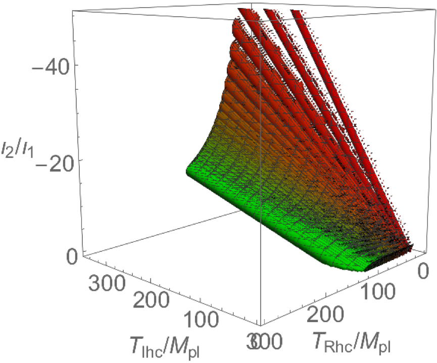
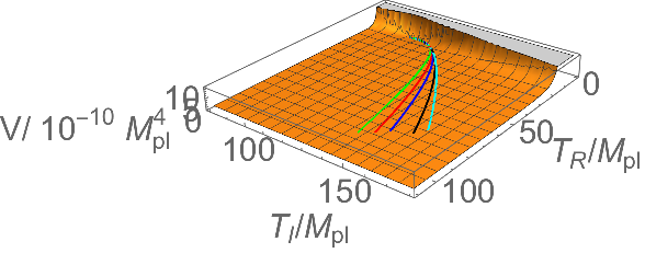
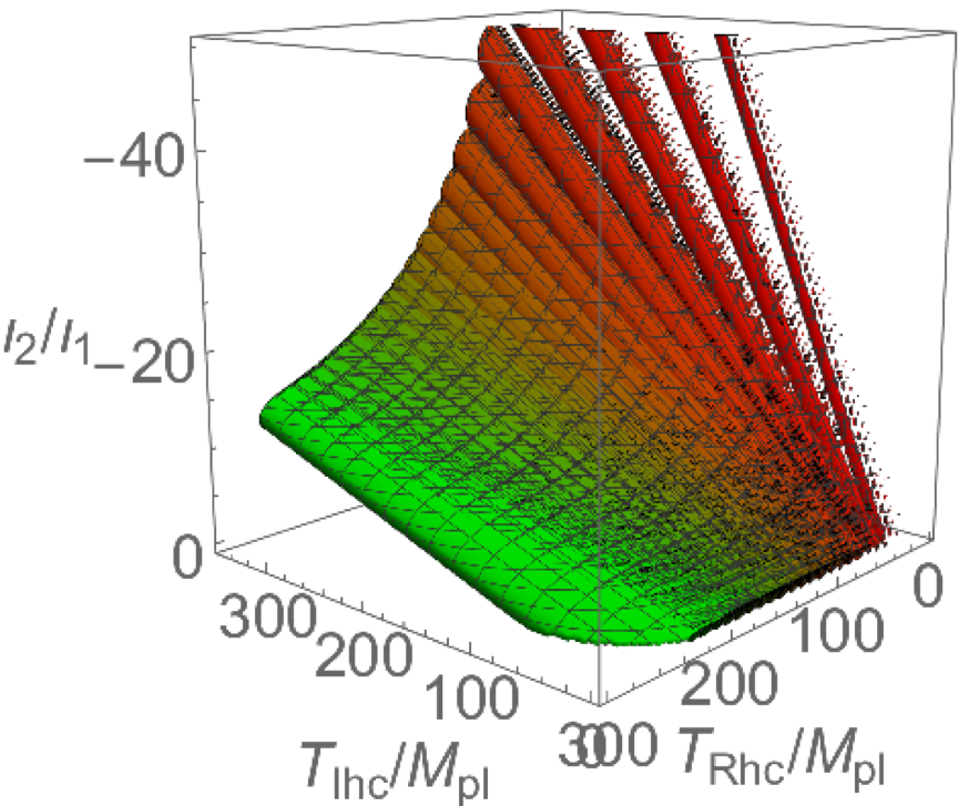
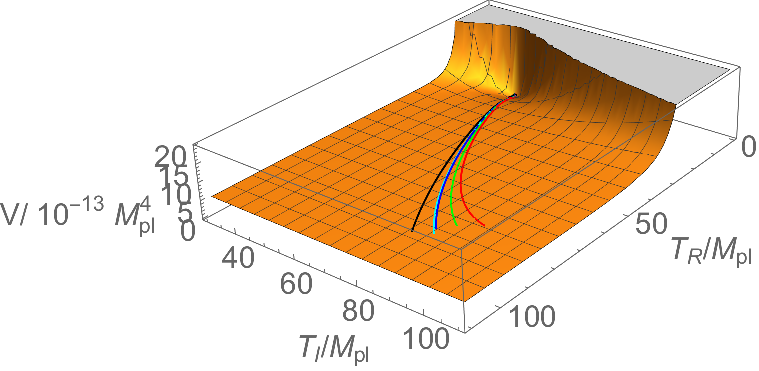
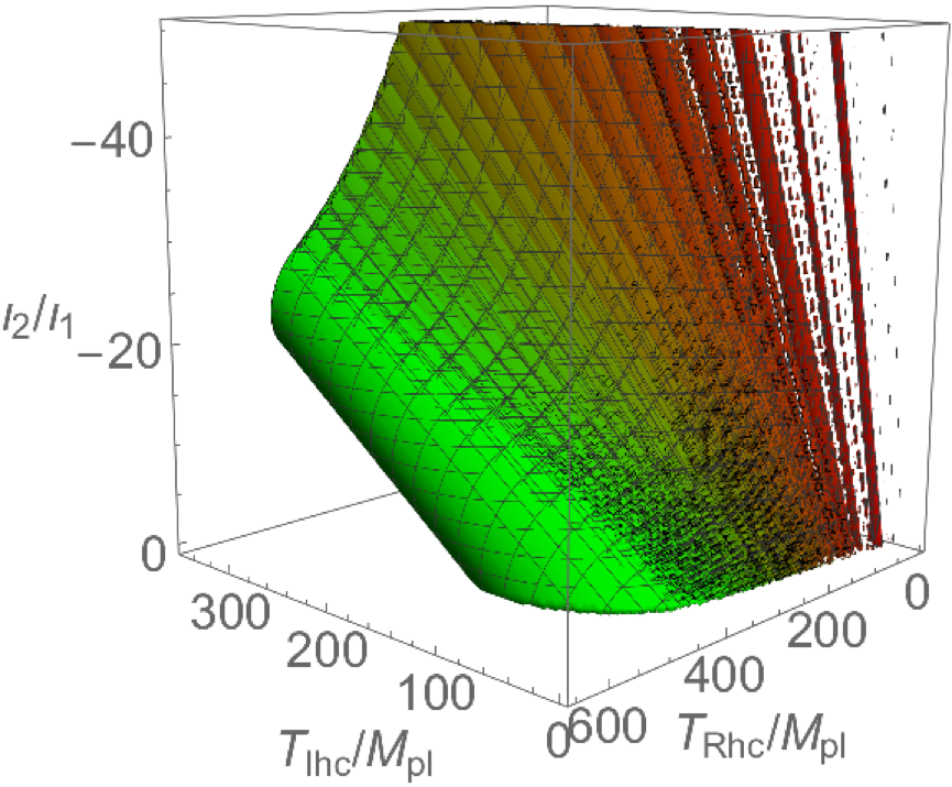
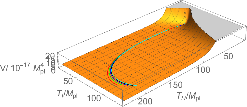
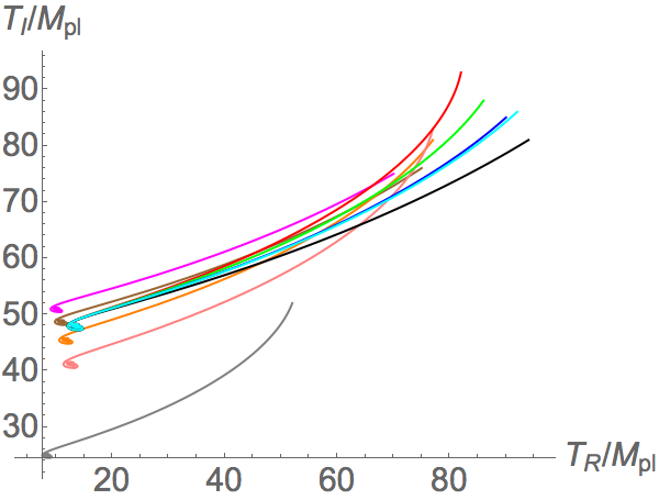
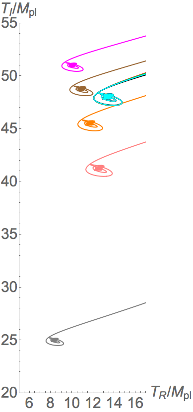
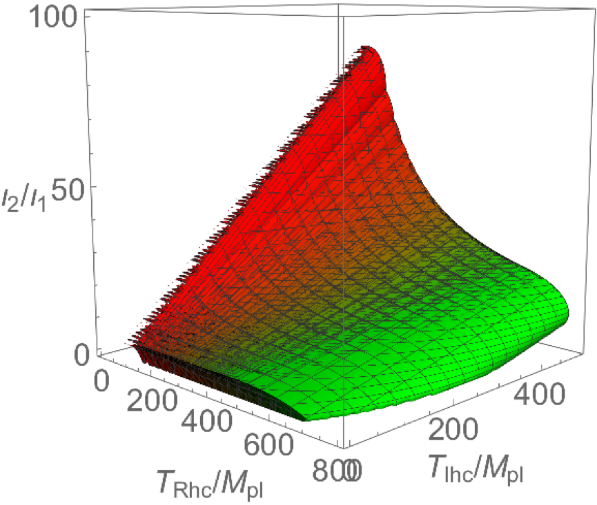
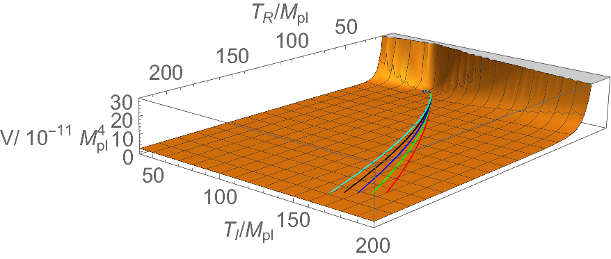
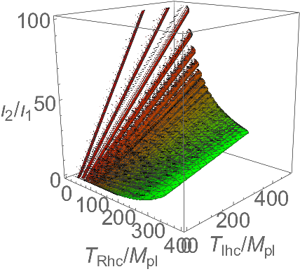
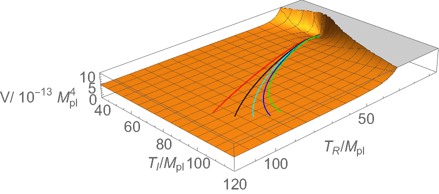
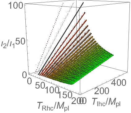
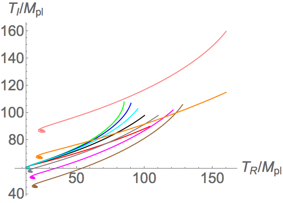
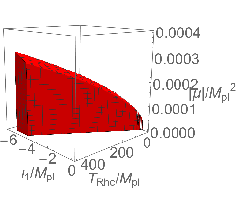
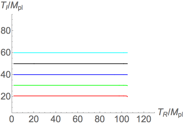
Figure 1: Left: Regions of possible values of ${T}_{R\text{hc}}$, ${T}_{I\text{hc}}$ ${\iota}_{2}/{\iota}_{1}$ for inflation based on the constraints listed in Table 1 at various integers ${\rho}$, a fixed $\left|{\mu}\right|=3\times{10}^{-4}{M}_{\text{pl}}^{2}$ and ${\omega}_{1}>0$ $\left({\iota}_{1}>0\right)$. Each ”C” shaped tube moves from red color to green color as ${\iota}_{1}$ increases. Please pay attention to the direction of magnitude of each axis in each graph. $1$st row: ${\rho}=4$, from ${\iota}_{1}=9{M}_{\text{pl}}$ (red) to ${\iota}_{1}=49{M}_{\text{pl}}$ (green) with an increment of $2{M}_{\text{pl}}$; $2$nd row: ${\rho}=5$, from ${\iota}_{1}=6{M}_{\text{pl}}$ (red) to ${\iota}_{1}=46{M}_{\text{pl}}$ (green) with an increment of $2{M}_{\text{pl}}$; $3$rd row: ${\rho}=6$, from ${\iota}_{1}=1{M}_{\text{pl}}$ (red) to ${\iota}_{1}=21{M}_{\text{pl}}$ (green) with an increment of $1{M}_{\text{pl}}$. (These regions are restricted by Table 1 only without the e-folding constraints $50\leq{N}_{\text{end}}-{N}_{\text{hc}}\leq 60$. ) Right: The trajectories of background fields on the potential surface. $1$st row: ${\rho}=4$, $2$nd row: ${\rho}=5$, $3$rd row: ${\rho}=6$. Various colors of the paths correspond to the parameter sets lised on Table 6, 6 and 8 respectively.

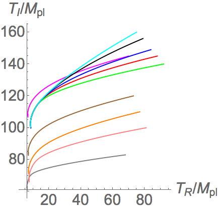
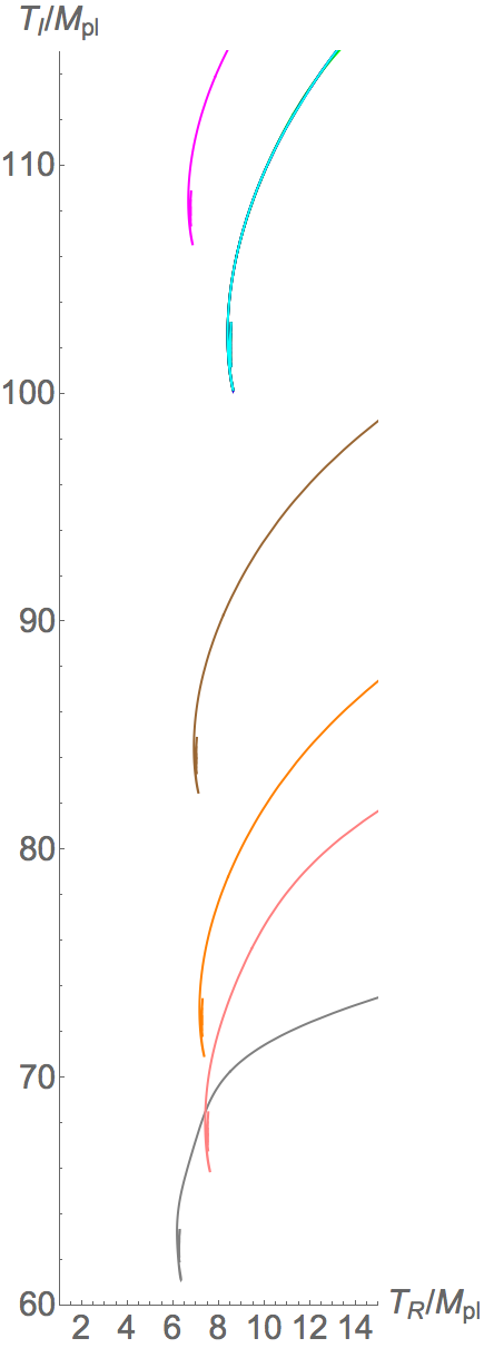
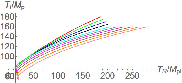
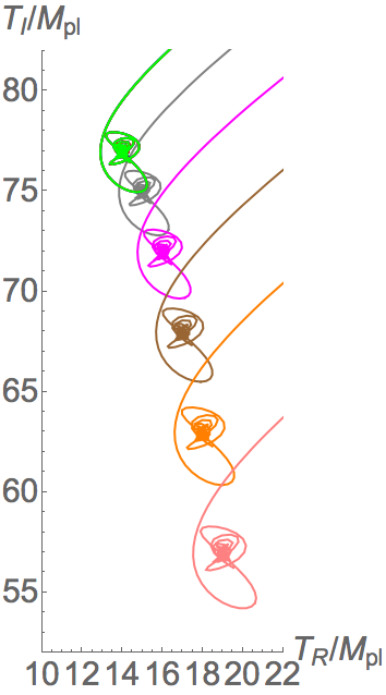
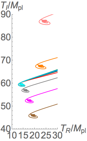
Figure 2: Evolution paths of inflation dynamics at ${\omega}_{1}>0\;\left({\iota}_{1}>0\right)$. $1$st row: ${\rho}=4$, $2$nd row: ${\rho}=5$, $3$rd row: ${\rho}=6$. Various colors refer to various parameter sets listed on Table 6, 6 and 8 correspondingly.

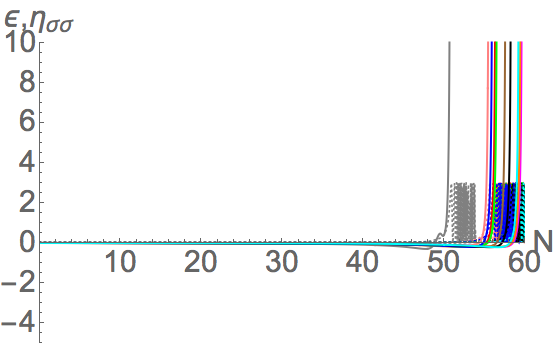
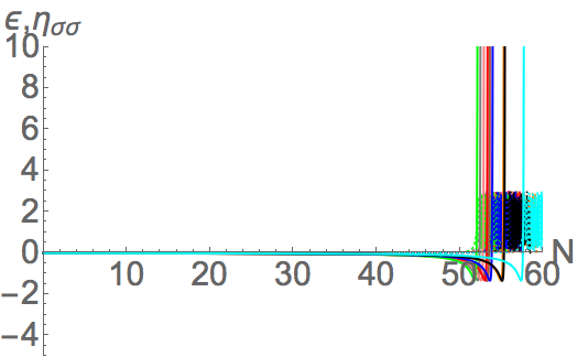
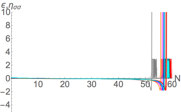
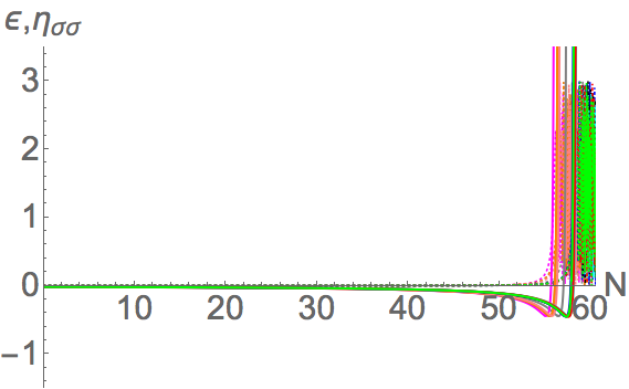
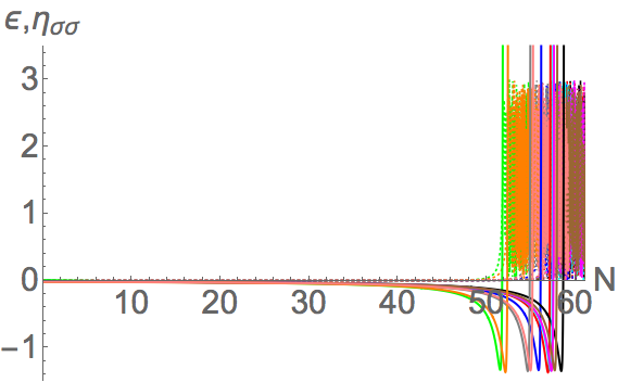
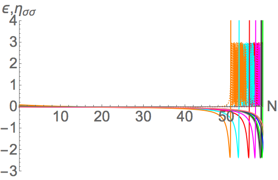
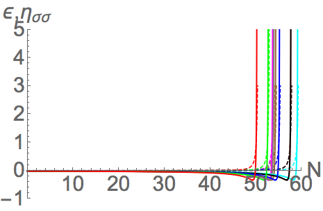
Figure 3: Evolutions of slow-roll parameters ${\epsilon}$ and ${\eta}_{\sigma\sigma}$ at ${\omega}_{1}>0\;\left({\iota}_{1}>0\right)$. $1$st row: ${\rho}=4$, $2$nd row: ${\rho}=5$, $3$rd row: ${\rho}=6$. Various colors refer to various parameter sets listed on Table 6, 6 and 8 correspondingly. Dotted lines represent the evolutions of $\epsilon$ while the solid lines represent the counterpart of ${\eta}_{{\sigma}{\sigma}}$.

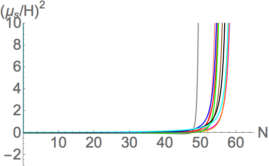
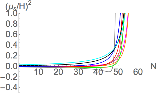
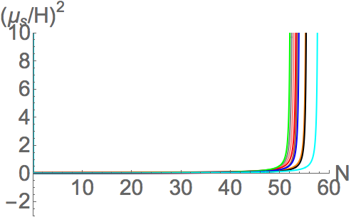
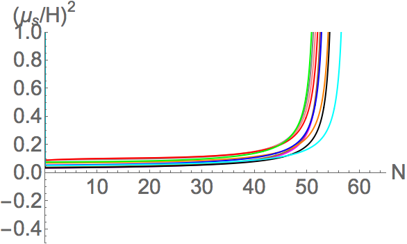
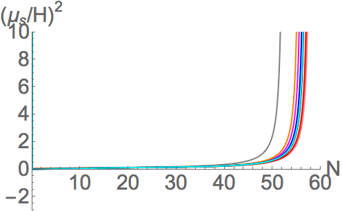
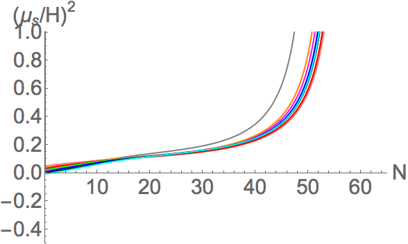
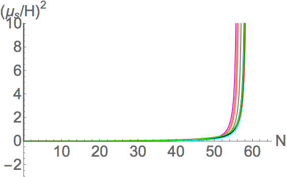
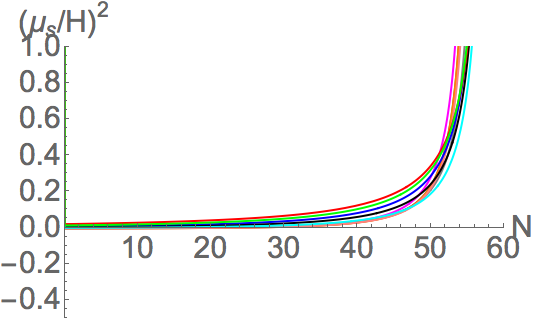
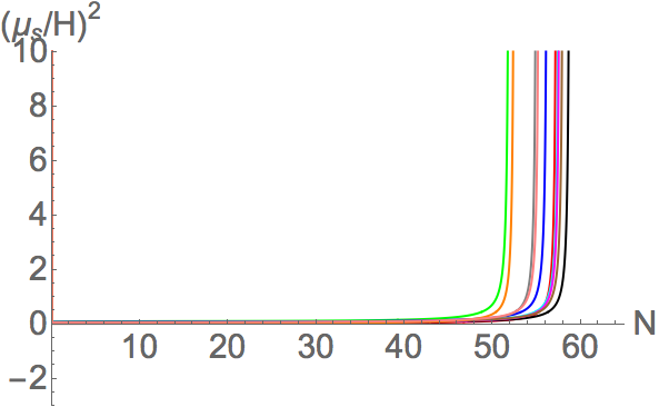
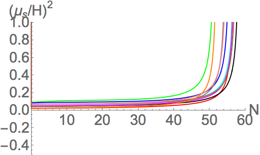
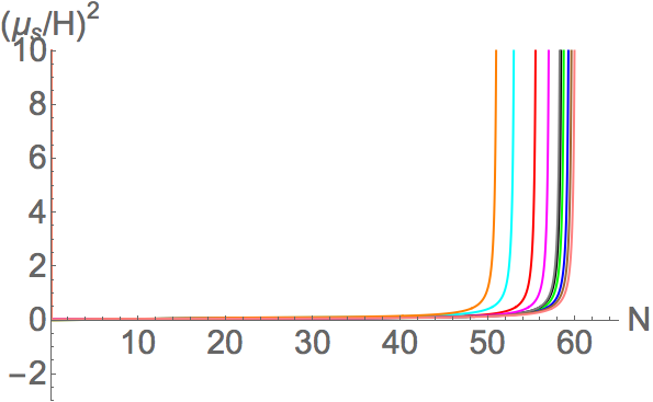
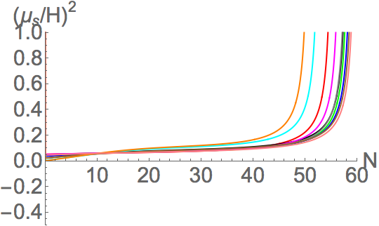
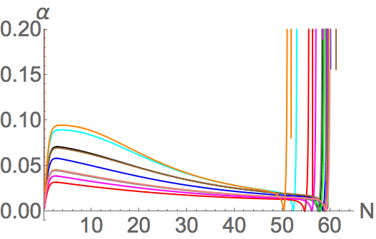
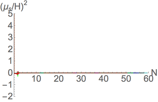
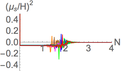
Figure 4: Square of effective mass per Hubble parameter $\left({\mu}_{s}/H\right)^{2}$ at ${\omega}_{1}>0\;\left({\iota}_{1}>0\right)$. $1$st row: ${\rho}=4$, $2$nd row: ${\rho}=5$, $3$rd row: ${\rho}=6$. The graphs on the right hand side (R.H.S.) are the close shots of that on the left hand side (L.H.S.) near zero. Various colors refer to various parameter sets listed on Table 6, 6 and 8 correspondingly.

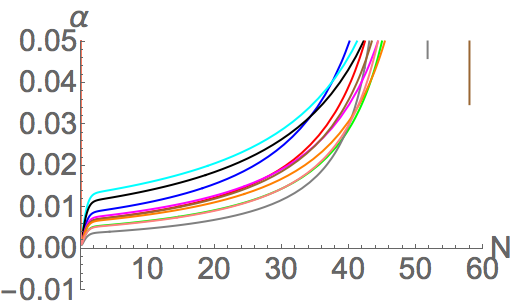
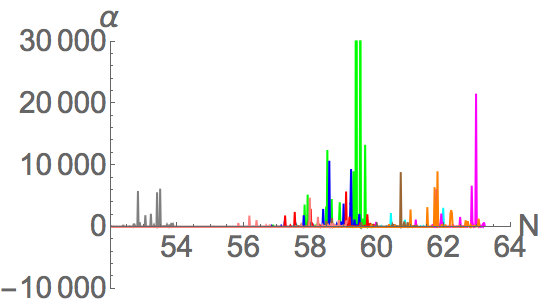
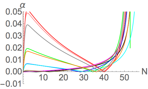
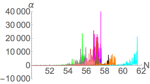
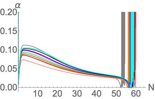
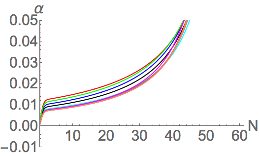
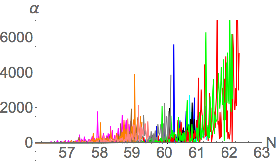
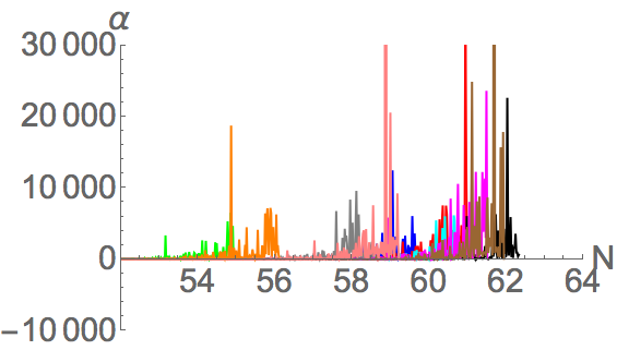
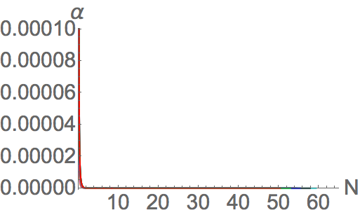
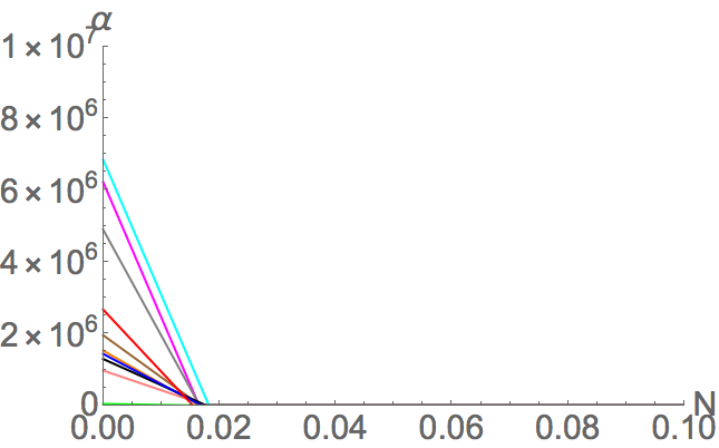
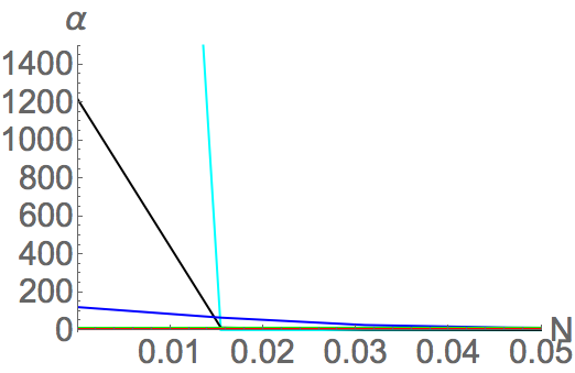
Figure 5: 2 times of turn rate per Hubble parameter ${\alpha}=2{\omega}/H$ at ${\omega}_{1}>0\;\left({\iota}_{1}>0\right)$. $1$st row: ${\rho}=4$, $2$nd row: ${\rho}=5$, $3$rd row: ${\rho}=6$. Left graphs show the overall evolutions, while right graphs focus on the changes at the end of inflation. Various colors refer to various parameter sets listed on Table 8, 10 and 10 correspondingly.

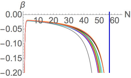
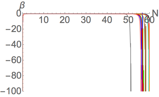
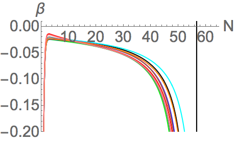
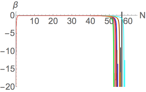
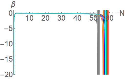
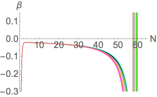
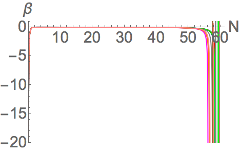
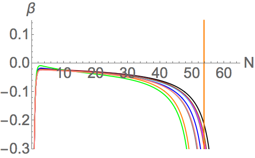
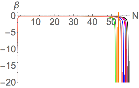
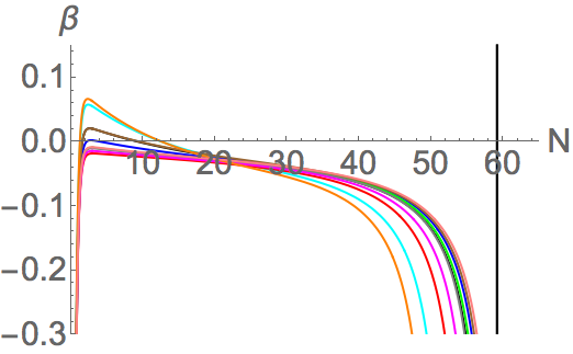
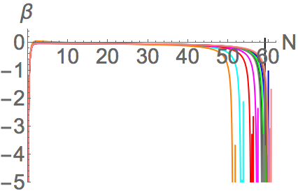
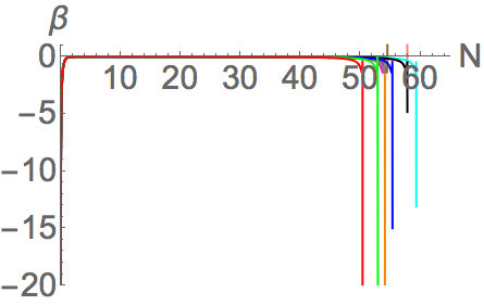
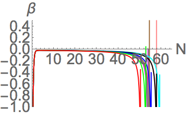
Figure 6: $\beta$ at ${\omega}_{1}>0\;\left({\iota}_{1}>0\right)$. $1$st row: ${\rho}=4$, $2$nd row: ${\rho}=5$, $3$rd row: ${\rho}=6$. The graphs on the right hand side (R.H.S.) are the close shots of that on the left hand side (L.H.S.). Various colors refer to various parameter sets listed on Table 8, 10 and 10 correspondingly.

In Figure 1, we show the possible positive values of ${T}_{R\text{hc}}$, ${T}_{I\text{hc}}$ and ${\iota}_{2}/{\iota}_{1}$ based on the Planck observation constraints listed in Table 1 at various ${\rho}=4,5,6$. The ”C” shape tube regions gradually change the color from red to green as ${\iota}_{1}$ gradually increases with a constant increment (For details, please refer to the description of Figure 1). We extract some of the possible parameters satisfying the e-folding constraints $50\leq{N}_{\text{end}}-{N}_{\text{hc}}\leq 60$ as listed in Table 6, 6 and 8, and their corresponding evolution paths are plotted in Figure 2. The colors correspond to the counterparts of the paths shown in Figure 2. One can see that for ${\rho}=4$, the background fields move towards their corresponding minimum point (dS vacuum point) in a nearly straight line, turn to the minimum point with a larger turn rate and then oscillate around the minimum point. As ${\rho}$ increases gradually up to $6$, the background fields greatly turn in the initial stage, move towards their corresponding minimum point and finally oscillate around the minimum point.

Next, in Figure 3, we can see the evolutions of $\epsilon$ and ${\eta}_{{\sigma}{\sigma}}$ of all the listed parameter sets in Table 6, 6 and 8. Basically, starting from very small positive values, all the $\epsilon$ (dotted) lines evolve and keep at a close-to-zero value, surge to 3 after $50$ e-folding and then oscillate between $0$ and $3$. Also, ${\eta}_{{\sigma}{\sigma}}$ (solid) lines start from a value very close to zero, evolve around zero and then sharply increase at the end of inflation. That means the background fields roll slowly initially and then run at an increasing rate, which is consistent with the mechanism of inflation. In Figure 4, after dropping sharply from a large positive value to a small positive value, the effective mass square of the entropy perturbation $\left({\mu}_{s}/H\right)^{2}$, which is given by Eq.(113), remains light and physical. This shows that the trajectories roll from the plateau. Since ${\mu}_{s}^{2}$ is related to the curvature of the potential in the direction orthogonal to the trajectory, light mass square means the curvature orthogonal to the trajectory is small at the initial stage. When the background fields roll off the ridge and reach $50$ e-folding, the entropy mass square largely grows because the curvature orthogonal to the trajectory is large and the turn rate becomes significant as the background field oscillates around their corresponding minimum points.

Color	${\iota}_{1}$	${\iota}_{2}/{\iota}_{1}$	${M}_{3/2-}/{M}_{\text{pl}}$	$\left.{F}_{T}\right|_{-}/{M}_{\text{pl}}$	${T}_{R\text{end}}$	${T}_{I\text{end}}$	${T}_{R\text{hc}}$	${T}_{I\text{hc}}$	${N}_{\text{end}}$	${N}_{\text{stop}}$	${\beta}_{\text{iso}}$	$\cos{\left(\Delta\right)}$
Gray	$25$	$-5$	$1.2\times{10}^{-4}$	$6.912\times{10}^{-5}$	$6.25$	$62.5$	$68$	$83$	$50.4485$	$53.8960$	$1.87873\times{10}^{-39}$	$2.2983\times{10}^{-5}$
Magenta	$27$	$-8$	$1.1111\times{10}^{-4}$	$5.9259\times{10}^{-5}$	$6.75$	$108$	$70$	$145$	$59.3514$	$63.2240$	$5.48281\times{10}^{-40}$	$2.86372\times{10}^{-5}$
Brown	$28$	$-6$	$1.0714\times{10}^{-4}$	$5.5102\times{10}^{-5}$	$7$	$84$	$73$	$120$	$57.3194$	$61.1881$	$5.32875\times{10}^{-39}$	$2.58454\times{10}^{-5}$
Orange	$29$	$-5$	$1.0344\times{10}^{-4}$	$5.1367\times{10}^{-5}$	$7.25$	$72.5$	$77$	$110$	$59.1943$	$63.0620$	$6.85479\times{10}^{-38}$	$2.52503\times{10}^{-5}$
Pink	$30$	$-4.5$	$5\times{10}^{-4}$	$4.8\times{10}^{-5}$	$7.5$	$67.5$	$81$	$100$	$55.2191$	$59.0726$	$1.11729\times{10}^{-39}$	$2.15684\times{10}^{-5}$
Red	$34$	$-6$	$4.41176\times{10}^{-4}$	$3.73702\times{10}^{-5}$	$8.5$	$102$	$88$	$145$	$56.0756$	$59.9293$	$5.14412\times{10}^{-37}$	$2.08999\times{10}^{-5}$
Green	$34$	$-6$	$4.41176\times{10}^{-4}$	$3.73702\times{10}^{-5}$	$8.5$	$102$	$92$	$140$	$56.2624$	$59.9871$	$1.35243\times{10}^{-42}$	$1.94259\times{10}^{-5}$
Blue	$34$	$-6$	$4.41176\times{10}^{-4}$	$3.73702\times{10}^{-5}$	$8.5$	$102$	$84$	$149$	$55.6707$	$59.5427$	$4.45289\times{10}^{-40}$	$2.29009\times{10}^{-5}$
Black	$34$	$-6$	$4.41176\times{10}^{-4}$	$3.73702\times{10}^{-5}$	$8.5$	$102$	$79$	$156$	$57.9958$	$61.0403$	$4.68586\times{10}^{-43}$	$3.08396\times{10}^{-5}$
Cyan	$34$	$-6$	$4.41176\times{10}^{-4}$	$3.73702\times{10}^{-5}$	$8.5$	$102$	$75$	$160$	$58.9596$	$62.0001$	$2.30095\times{10}^{-41}$	$4.50112\times{10}^{-5}$

Table 5: Feasible parameter sets for inflation for ${\omega}_{1}>0$ (or ${\iota}_{1}>0$) and ${\rho}=4$. Recall the unit of each variable is the following. $\left[{\iota}_{1}\right]={M}_{\text{pl}}$, $\left[{M}_{3/2-}\right]={M}_{\text{pl}}$, $\left[\left.{F}_{T}\right|_{-}\right]={M}_{\text{pl}}^{2}$, $\left[{T}_{R\text{end}}\right]=\left[{T}_{I\text{end}}\right]=\left[{T}_{R\text{hc}}\right]=\left[{T}_{I\text{hc}}\right]={M}_{\text{pl}}$. ${N}_{\text{end}}$ is the e-folding number when ${\epsilon}=1$, which represents the end of inflation. ${N}_{\text{stop}}$ means the e-folding number that we stop the numerical calculation.

Color	${\iota}_{1}$	${\iota}_{2}/{\iota}_{1}$	${M}_{3/2-}/{10}^{-5}{M}_{\text{pl}}$	$\left.{F}_{T}\right|_{-}/{10}^{-5}{M}_{\text{pl}}^{2}$	${T}_{R\text{end}}$	${T}_{I\text{end}}$	${T}_{R\text{hc}}$	${T}_{I\text{hc}}$	${N}_{\text{end}}$	${N}_{\text{stop}}$	${\beta}_{\text{iso}}$	$\cos{\left(\Delta\right)}$
Gray	$10$	$-5$	$19.7028$	$2.47431$	$8.3333$	$25$	$52$	$52$	$52.3575$	$55.9694$	$2.66698\times{10}^{-36}$	$5.87517\times{10}^{-5}$
Magenta	$12$	$-8.5$	$14.9884$	$1.56856$	$10$	$51$	$70$	$75$	$53.4696$	$57.5777$	$2.34071\times{10}^{-38}$	$7.95594\times{10}^{-5}$
Brown	$13$	$-7.5$	$13.2927$	$1.28409$	$10.8333$	$48.75$	$75$	$76$	$53.4769$	$57.4120$	$3.60886\times{10}^{-38}$	$9.36358\times{10}^{-5}$
Orange	$14$	$-6.5$	$11.8942$	$1.0669$	$11.6667$	$45.5$	$77$	$81$	$55.1485$	$59.2092$	$1.17279\times{10}^{-37}$	$1.31272\times{10}^{-4}$
Pink	$15$	$-5.5$	$10.7249$	$0.897895$	$12.5$	$41.25$	$77$	$83$	$52.765$	$56.8757$	$4.02109\times{10}^{-35}$	$3.01275\times{10}^{-5}$
Red	$16$	$-6$	$9.73528$	$0.764106$	$13.3333$	$48$	$82$	$93$	$53.206$	$57.3168$	$2.04007\times{10}^{-36}$	$2.65296\times{10}^{-5}$
Green	$16$	$-6$	$9.73528$	$0.764106$	$13.3333$	$48$	$86$	$88$	$51.9849$	$55.8550$	$5.58572\times{10}^{-37}$	$9.72256\times{10}^{-5}$
Blue	$16$	$-6$	$9.73528$	$0.764106$	$13.3333$	$48$	$90$	$85$	$53.8209$	$57.6154$	$2.09012\times{10}^{-38}$	$2.90824\times{10}^{-4}$
Black	$16$	$-6$	$9.73528$	$0.764106$	$13.3333$	$48$	$94$	$81$	$55.2881$	$58.4560$	$7.36786\times{10}^{-37}$	$6.65673\times{10}^{-5}$
Cyan	$16$	$-6$	$9.73528$	$0.764106$	$13.3333$	$48$	$92$	$86$	$57.56$	$61.5649$	$2.27647\times{10}^{-39}$	$3.40788\times{10}^{-4}$

Table 6: Feasible parameter sets for inflation for ${\omega}_{1}>0$ (or ${\iota}_{1}>0$) and ${\rho}=5$. Recall the unit of each variable is the following. $\left[{\iota}_{1}\right]={M}_{\text{pl}}$, $\left[{M}_{3/2-}\right]={M}_{\text{pl}}$, $\left[\left.{F}_{T}\right|_{-}\right]={M}_{\text{pl}}^{2}$, $\left[{T}_{R\text{end}}\right]=\left[{T}_{I\text{end}}\right]=\left[{T}_{R\text{hc}}\right]=\left[{T}_{I\text{hc}}\right]={M}_{\text{pl}}$. ${N}_{\text{end}}$ is the e-folding number when ${\epsilon}=1$, which represents the end of inflation. ${N}_{\text{stop}}$ means the e-folding number that we stop the numerical calculation.

Color	${\iota}_{1}$	${\iota}_{2}/{\iota}_{1}$	${M}_{3/2-}/{10}^{-5}{M}_{\text{pl}}$	$\left.{F}_{T}\right|_{-}/{10}^{-5}{M}_{\text{pl}}^{2}$	${T}_{R\text{end}}$	${T}_{I\text{end}}$	${T}_{R\text{hc}}$	${T}_{I\text{hc}}$	${N}_{\text{end}}$	${N}_{\text{stop}}$	${\beta}_{\text{iso}}$	$\cos{\left(\Delta\right)}$
Gray	$3$	$-5$	$5.0114$	$0.3251$	$13.5$	$7.5$	$66$	$30$	$52.2627$	$54.3395$	$2.39368\times{10}^{-37}$	$8.4469\times{10}^{-6}$
Magenta	$4$	$-6$	$2.81893$	$0.1372$	$18$	$12$	$92$	$40$	$56.1668$	$58.2761$	$6.7651\times{10}^{-37}$	$9.20973\times{10}^{-6}$
Brown	$5$	$-7$	$1.8041$	$0.07023$	$22.5$	$17.5$	$118$	$50$	$57.7282$	$59.8035$	$5.1486\times{10}^{-38}$	$9.9622\times{10}^{-6}$
Orange	$6$	$-8$	$1.2529$	$0.04064$	$27$	$24$	$142$	$60$	$55.6072$	$57.7068$	$5.51104\times{10}^{-39}$	$1.01895\times{10}^{-5}$
Pink	$7$	$-9$	$0.920467$	$0.0255952$	$31.5$	$31.5$	$170$	$70$	$57.8876$	$59.9947$	$3.22952\times{10}^{-40}$	$1.2694\times{10}^{-5}$
Red	$9$	$-10$	$0.556826$	$0.0120427$	$40.5$	$45$	$214$	$101$	$57.5722$	$59.6827$	$2.29669\times{10}^{-41}$	$6.38619\times{10}^{-6}$
Green	$9$	$-10$	$0.556826$	$0.0120427$	$40.5$	$45$	$210$	$105$	$56.6762$	$58.7541$	$4.01603\times{10}^{-37}$	$4.91618\times{10}^{-6}$
Blue	$9$	$-10$	$0.556826$	$0.0120427$	$40.5$	$45$	$206$	$110$	$56.6968$	$58.8117$	$7.46009\times{10}^{-38}$	$3.73375\times{10}^{-6}$
Black	$9$	$-10$	$0.556826$	$0.0120427$	$40.5$	$45$	$202$	$115$	$57.0605$	$59.1691$	$3.21796\times{10}^{-39}$	$2.89628\times{10}^{-6}$
Cyan	$9$	$-10$	$0.556826$	$0.0120427$	$40.5$	$45$	$199$	$118$	$56.9827$	$59.0902$	$5.66193\times{10}^{-39}$	$2.46863\times{10}^{-6}$

Table 7: Feasible parameter sets for inflation for ${\omega}_{1}>0$ (or ${\iota}_{1}>0$) and ${\rho}=6$. Recall the unit of each variable is the following. $\left[{\iota}_{1}\right]={M}_{\text{pl}}$, $\left[{M}_{3/2-}\right]={M}_{\text{pl}}$, $\left[\left.{F}_{T}\right|_{-}\right]={M}_{\text{pl}}^{2}$, $\left[{T}_{R\text{end}}\right]=\left[{T}_{I\text{end}}\right]=\left[{T}_{R\text{hc}}\right]=\left[{T}_{I\text{hc}}\right]={M}_{\text{pl}}$. ${N}_{\text{end}}$ is the e-folding number when ${\epsilon}=1$, which represents the end of inflation. ${N}_{\text{stop}}$ means the e-folding number that we stop the numerical calculation.

Color	${\iota}_{1}$	${\iota}_{2}/{\iota}_{1}$	${M}_{3/2+}/{10}^{-6}{M}_{\text{pl}}$	${T}_{R\text{end}}$	${T}_{I\text{end}}$	${T}_{R\text{hc}}$	${T}_{I\text{hc}}$	${N}_{\text{end}}$	${N}_{\text{stop}}$	${\beta}_{\text{iso}}$	$\cos{\left(\Delta\right)}$
Red	$-14$	$11$	$2.67857$	$14$	$77$	$185$	$180$	$58.3165$	$62.6594$	$9.9157\times{10}^{-40}$	$1.31875\times{10}^{-5}$
Green	$-14$	$11$	$2.67857$	$14$	$77$	$190$	$175$	$58.1038$	$62.4462$	$4.82523\times{10}^{-39}$	$1.14167\times{10}^{-5}$
Blue	$-14$	$11$	$2.67857$	$14$	$77$	$195$	$170$	$58.0405$	$61.3501$	$3.07253\times{10}^{-40}$	$1.02649\times{10}^{-5}$
Black	$-14$	$11$	$2.67857$	$14$	$77$	$200$	$165$	$58.1267$	$61.4364$	$1.49867\times{10}^{-40}$	$9.46949\times{10}^{-6}$
Cyan	$-14$	$11$	$2.67857$	$14$	$77$	$205$	$160$	$58.3628$	$61.6725$	$6.49472\times{10}^{-38}$	$8.89825\times{10}^{-6}$
Gray	$-15$	$10$	$2.5$	$150$	$75$	$220$	$160$	$57.2553$	$60.5650$	$7.23189\times{10}^{-35}$	$7.98833\times{10}^{-6}$
Magenta	$-16$	$9$	$2.34375$	$144$	$72$	$233$	$160$	$55.8962$	$59.2060$	$2.04449\times{10}^{-35}$	$7.30653\times{10}^{-6}$
Brown	$-17$	$8$	$2.20588$	$136$	$68$	$250$	$160$	$56.3214$	$59.6312$	$2.21076\times{10}^{-39}$	$6.80653\times{10}^{-6}$
Orange	$-18$	$7$	$2.08333$	$126$	$63$	$265$	$160$	$56.3138$	$59.6237$	$3.33083\times{10}^{-36}$	$6.41033\times{10}^{-6}$
Pink	$-19$	$6$	$1.97368$	$114$	$57$	$280$	$160$	$56.5409$	$59.8508$	$4.60472\times{10}^{-36}$	$6.10035\times{10}^{-6}$

Table 8: Feasible parameter sets for inflation for ${\omega}_{1}<0$ (or ${\iota}_{1}<0$) and ${\rho}=4$. Note that the $F$ term SUSY breaking scale is $0$ for all real values of parameters and fields. Recall the unit of each variable is the following. $\left[{\iota}_{1}\right]={M}_{\text{pl}}$, $\left[{M}_{3/2+}\right]={M}_{\text{pl}}$, $\left[{T}_{R\text{end}}\right]=\left[{T}_{I\text{end}}\right]=\left[{T}_{R\text{hc}}\right]=\left[{T}_{I\text{hc}}\right]={M}_{\text{pl}}$. ${N}_{\text{end}}$ is the e-folding number when ${\epsilon}=1$, which represents the end of inflation. ${N}_{\text{stop}}$ means the e-folding number that we stop the numerical calculation.

6.1.2 Suppose ${\omega}_{1}<0,\;{\rho}>3$.

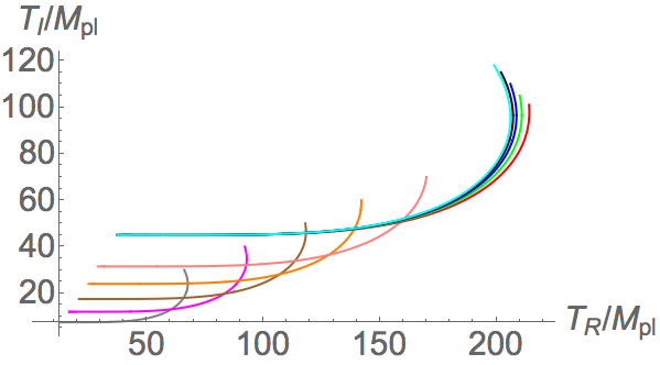
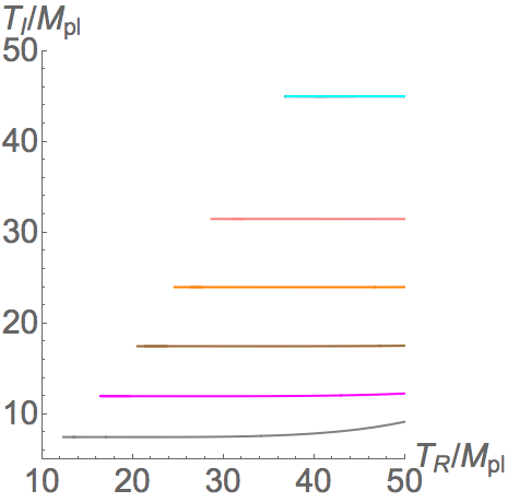
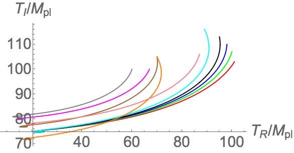
Figure 7: Left: Regions of possible values of ${T}_{R\text{hc}}$, ${T}_{I\text{hc}}$ ${\iota}_{2}/{\iota}_{1}$ for inflation based on the constraints listed in Table 1 at various integers ${\rho}$, a fixed $\left|{\mu}\right|=3\times{10}^{-4}{M}_{\text{pl}}^{2}$ and ${\omega}_{1}<0$ $\left({\iota}_{1}<0\right)$. Each ”C” like cylinder moves from red color to green color as ${\iota}_{1}$ increases. Please pay attention to the direction of magnitude of each axis in each graph. $1$st row: ${\rho}=4$, from ${\iota}_{1}=-12{M}_{\text{pl}}$ (red) to ${\iota}_{1}=-52{M}_{\text{pl}}$ (green) with an increment of $2{M}_{\text{pl}}$; $2$nd row: ${\rho}=5$, from ${\iota}_{1}=-6{M}_{\text{pl}}$ (red) to ${\iota}_{1}=-46{M}_{\text{pl}}$ (green) with an increment of $2{M}_{\text{pl}}$; $3$rd row: ${\rho}=6$, from ${\iota}_{1}=-6{M}_{\text{pl}}$ (red) to ${\iota}_{1}=-46{M}_{\text{pl}}$ (green) with an increment of $2{M}_{\text{pl}}$. (These regions are restricted by Table 1 only without the e-folding constraints $50\leq{N}_{\text{end}}-{N}_{\text{hc}}\leq 60$. ) Right: The trajectories of background fields on the potential surface. $1$st row: ${\rho}=4$, $2$nd row: ${\rho}=5$, $3$rd row: ${\rho}=6$. Various colors of the paths correspond to the parameter sets lised on Table 8, 10 and 10 respectively.

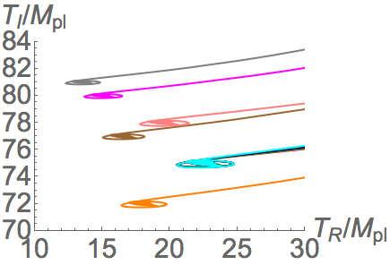
Figure 8: Evolution paths of inflation dynamics at ${\omega}_{1}<0\;\left({\iota}_{1}<0\right)$. $1$st row: ${\rho}=4$, $2$nd row: ${\rho}=5$, $3$rd row: ${\rho}=6$. Various colors refer to various parameter sets listed on Table 8, 10 and 10 correspondingly.

Figure 9: Evolutions of slow-roll parameters at ${\omega}_{1}<0\;\left({\iota}_{1}<0\right)$. $1$st row: ${\rho}=4$, $2$nd row: ${\rho}=5$, $3$rd row: ${\rho}=6$. Various colors refer to various parameter sets listed on Table 8, 10 and 10 correspondingly. Dotted lines represent the evolutions of $\epsilon$ while the solid lines represent the counterpart of ${\eta}_{{\sigma}{\sigma}}$.

Figure 10: Square of effective mass per Hubble parameter $\left({\mu}_{s}/H\right)^{2}$ at ${\omega}_{1}<0\;\left({\iota}_{1}<0\right)$. $1$st row: ${\rho}=4$, $2$nd row: ${\rho}=5$, $3$rd row: ${\rho}=6$. The graphs on the right hand side (R.H.S.) are the close shots of that on the left hand side (L.H.S.) near zero. Various colors refer to various parameter sets listed on Table 8, 10 and 10 correspondingly.

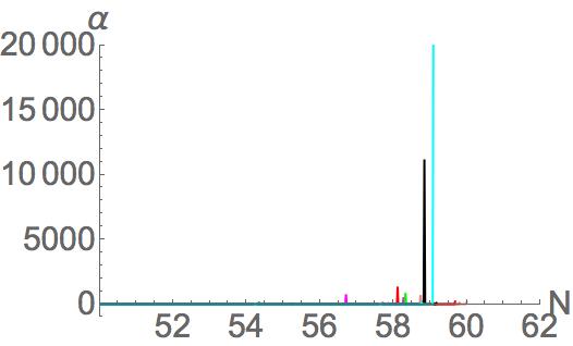
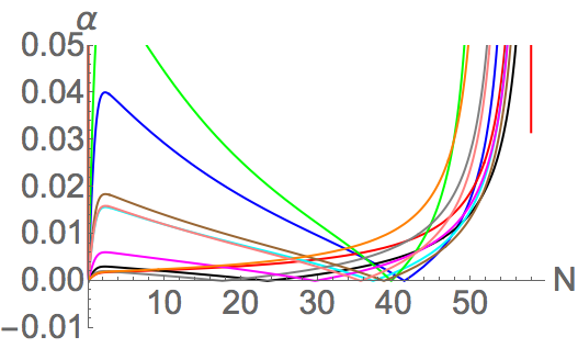
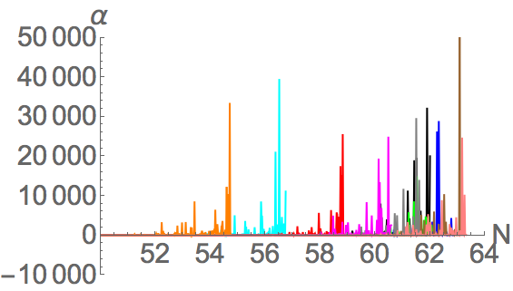
Figure 11: 2 times of turn rate per Hubble parameter ${\alpha}=2{\omega}/H$ at ${\omega}_{1}<0\;\left({\iota}_{1}<0\right)$. $1$st row: ${\rho}=4$, $2$nd row: ${\rho}=5$, $3$rd row: ${\rho}=6$. The graphs on the right hand side (R.H.S.) are the close shots of that on the left hand side (L.H.S.). Various colors refer to various parameter sets listed on Table 8, 10 and 10 correspondingly. Left graphs show the overall evolutions, while right graphs are the closed shots at the end of inflation.

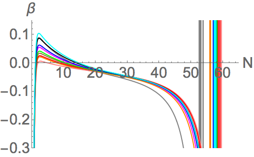
Figure 12: $\beta$ at ${\omega}_{1}<0\;\left({\iota}_{1}<0\right)$. $1$st row: ${\rho}=4$, $2$nd row: ${\rho}=5$, $3$rd row: ${\rho}=6$. The graphs on the right hand side (R.H.S.) are the close shots of that on the left hand side (L.H.S.). Various colors refer to various parameter sets listed on Table 8, 10 and 10 correspondingly.

Color	${\iota}_{1}$	${\iota}_{2}/{\iota}_{1}$	${M}_{3/2+}/{10}^{-7}{M}_{\text{pl}}$	${T}_{R\text{end}}$	${T}_{I\text{end}}$	${T}_{R\text{hc}}$	${T}_{I\text{hc}}$	${N}_{\text{end}}$	${N}_{\text{stop}}$	${\beta}_{\text{iso}}$	$\cos{\left(\Delta\right)}$
Red	$-17$	$7$	$3.97837$	$14.1667$	$59.5$	$104$	$90$	$57.1196$	$61.1125$	$3.38902\times{10}^{-38}$	$4.03578\times{10}^{-5}$
Green	$-17$	$7$	$3.97837$	$14.1667$	$59.5$	$85$	$108$	$51.7453$	$54.9271$	$3.61843\times{10}^{-37}$	$1.98477\times{10}^{-5}$
Blue	$-17$	$7$	$3.97837$	$14.1667$	$59.5$	$90$	$107$	$56.0768$	$59.6890$	$8.03244\times{10}^{-37}$	$3.27246\times{10}^{-5}$
Black	$-17$	$7$	$3.97837$	$14.1667$	$59.5$	$100$	$98$	$58.6238$	$62.3304$	$7.06245\times{10}^{-41}$	$1.10696\times{10}^{-4}$
Cyan	$-17$	$7$	$3.97837$	$14.1667$	$59.5$	$95$	$103$	$57.4204$	$60.9148$	$1.34988\times{10}^{-37}$	$1.23669\times{10}^{-4}$
Gray	$-19$	$6$	$3.36704$	$95$	$57$	$110$	$98$	$54.8516$	$58.5579$	$3.8036\times{10}^{-39}$	$7.51476\times{10}^{-5}$
Magenta	$-21$	$5$	$2.89767$	$87.5$	$52.5$	$121$	$102$	$57.5109$	$61.5113$	$7.10984\times{10}^{-38}$	$2.02087\times{10}^{-4}$
Brown	$-23$	$4$	$2.52805$	$76.6667$	$46$	$128$	$106$	$57.8894$	$61.9445$	$2.08549\times{10}^{-37}$	$6.69631\times{10}^{-5}$
Orange	$-27$	$5$	$1.98762$	$112.5$	$67.5$	$160$	$115$	$52.3259$	$56.1155$	$6.41039\times{10}^{-37}$	$2.44855\times{10}^{-5}$
Pink	$-29$	$6$	$1.78559$	$145$	$87$	$160$	$160$	$55.1624$	$59.2207$	$3.48978\times{10}^{-36}$	$7.42136\times{10}^{-5}$

Table 9: Feasible parameter sets for inflation for ${\omega}_{1}<0$ (or ${\iota}_{1}<0$) and ${\rho}=5$. Note that the $F$ term SUSY breaking scale is $0$ for all real values of parameters and fields. Recall the unit of each variable is the following. $\left[{\iota}_{1}\right]={M}_{\text{pl}}$, $\left[{M}_{3/2+}\right]={M}_{\text{pl}}$, $\left[{T}_{R\text{end}}\right]=\left[{T}_{I\text{end}}\right]=\left[{T}_{R\text{hc}}\right]=\left[{T}_{I\text{hc}}\right]={M}_{\text{pl}}$. ${N}_{\text{end}}$ is the e-folding number when ${\epsilon}=1$, which represents the end of inflation. ${N}_{\text{stop}}$ means the e-folding number that we stop the numerical calculation.

Color	${\iota}_{1}$	${\iota}_{2}/{\iota}_{1}$	${M}_{3/2+}/{10}^{-8}{M}_{\text{pl}}$	${T}_{R\text{end}}$	${T}_{I\text{end}}$	${T}_{R\text{hc}}$	${T}_{I\text{hc}}$	${N}_{\text{end}}$	${N}_{\text{stop}}$	${\beta}_{\text{iso}}$	$\cos{\left(\Delta\right)}$
Gray	$-18$	$9$	$6.85871$	$121.5$	$81$	$60$	$100$	$58.2101$	$61.6281$	$8.06083\times{10}^{-35}$	$6.77743\times{10}^{-5}$
Magenta	$-20$	$8$	$5.55556$	$120$	$80$	$67$	$100$	$56.9523$	$60.5887$	$7.4834\times{10}^{-35}$	$8.14647\times{10}^{-5}$
Brown	$-22$	$7$	$4.59137$	$115.5$	$77$	$70$	$105$	$59.5551$	$63.1895$	$2.44999\times{10}^{-35}$	$1.01176\times{10}^{-5}$
Orange	$-24$	$6$	$3.85802$	$108$	$72$	$70$	$105$	$50.9481$	$54.7494$	$2.71462\times{10}^{-35}$	$1.01176\times{10}^{-5}$
Pink	$-26$	$6$	$3.28731$	$117$	$78$	$87$	$106$	$59.907$	$63.3246$	$5.44139\times{10}^{-37}$	$4.42432\times{10}^{-5}$
Red	$-30$	$5$	$2.46914$	$22.5$	$75$	$101$	$103$	$55.4472$	$58.8651$	$4.7257\times{10}^{-37}$	$8.54936\times{10}^{-5}$
Green	$-30$	$5$	$2.46914$	$22.5$	$75$	$100$	$107$	$58.682$	$62.0998$	$3.2964\times{10}^{-37}$	$3.88947\times{10}^{-5}$
Blue	$-30$	$5$	$2.46914$	$22.5$	$75$	$98$	$110$	$59.2057$	$62.8400$	$1.28312\times{10}^{-34}$	$2.44867\times{10}^{-5}$
Black	$-30$	$5$	$2.46914$	$22.5$	$75$	$95$	$113$	$58.3676$	$62.0021$	$1.44804\times{10}^{-36}$	$1.58228\times{10}^{-5}$
Cyan	$-30$	$5$	$2.46914$	$22.5$	$75$	$89$	$116$	$52.9635$	$56.7473$	$1.58416\times{10}^{-34}$	$9.00233\times{10}^{-6}$

Table 10: Feasible parameter sets for inflation for ${\omega}_{1}<0$ (or ${\iota}_{1}<0$) and ${\rho}=6$. Note that the $F$ term SUSY breaking scale is $0$ for all real values of parameters and fields. Recall the unit of each variable is the following. $\left[{\iota}_{1}\right]={M}_{\text{pl}}$, $\left[{M}_{3/2+}\right]={M}_{\text{pl}}$, $\left[{T}_{R\text{end}}\right]=\left[{T}_{I\text{end}}\right]=\left[{T}_{R\text{hc}}\right]=\left[{T}_{I\text{hc}}\right]={M}_{\text{pl}}$. ${N}_{\text{end}}$ is the e-folding number when ${\epsilon}=1$, which represents the end of inflation. ${N}_{\text{stop}}$ means the e-folding number that we stop the numerical calculation.

Similar to the cases ${\omega}_{1}>0$, in Figure 7, we show the possible positive values of ${T}_{R\text{hc}}$, ${T}_{I\text{hc}}$ and ${\iota}_{2}/{\iota}_{1}$ based on the Planck observation constraints listed in Table 1 at various ${\rho}=4,5,6$. The ”C” shape tube regions gradually change the color from red to green as ${\iota}_{1}$ gradually decreases with a constant increment (For details, please refer to the description of Figure 7). We also extract some of the possible parameters satisfying the e-folding constraints $50\leq{N}_{\text{end}}-{N}_{\text{hc}}\leq 60$ as listed in Table 8, 10 and 10, and their corresponding evolution paths are plotted in Figure 8. One can see that for ${\rho}=4$, the paths move towards their corresponding minimum point (dS vacuum point) in a nearly a straight line, turn to the minimum point with a larger turn rate and then oscillate around the minimum point. However, the extent of turning is smaller than that of the evolution paths at ${\omega}_{1}>0$ and ${\rho}=4$. As ${\rho}$ increases gradually up to $6$, the paths change its shape into the form like turning greatly in the initial stage, moving towards their corresponding minimum point and finally oscillating around the minimum point.

Next, in Figure 9, we can see the evolutions of $\epsilon$ and ${\eta}_{{\sigma}{\sigma}}$ of all the listed parameter sets in Table 8, 10 and 10. Basically, starting from very small positive values, all the $\epsilon$ (dotted) lines evolve and keep at a close-to-zero value, surge to 3 after $50$ e-folding and then oscillate between $0$ and $3$. Also, ${\eta}_{{\sigma}{\sigma}}$ lines start from a value very close to zero, evolve around zero and then sharply increase at the end of inflation. In Figure 4, after dropping sharply from a large positive value to a small positive value, the effective mass square of the entropy perturbation $\left({\mu}_{s}/H\right)^{2}$ remains light and physical. This shows that the trajectory rolls from the plateau, where the field space curvature orthogonal to the trajectory is small in the initial stage, to the minimum point, where the entropy mass square largely grows.

6.2 Suppose ${\rho}=3$.

Figure 13: Left: A region of possible values of ${T}_{R\text{hc}}/{M}_{\text{pl}}$, ${\iota}_{1}/{M}_{\text{pl}}$ and $\left|{\mu}\right|/{M}_{\text{pl}}^{2}$ for inflation based on the constraints listed in Table 1. Right: The evolution of background fields on the potential surface. The colors of the lines correspond to the parameter sets listed in Table 1.

Figure 14: Evolution paths of inflation dynamics at ${\rho}=3$. Various colors refer to various parameter sets listed on Table 12.

Figure 15: Evolutions of slow-roll parameters ${\epsilon}$ and ${\eta}_{{\sigma}{\sigma}}$ for ${\rho}=3$. Various colors refer to various parameter sets listed on Table 12. Dotted lines represent the evolutions of $\epsilon$ while the solid lines represent the counterpart of ${\eta}_{{\sigma}{\sigma}}$.

Figure 16: Left: Evolutions of the turn rate per Hubble parameter ${\alpha}\left(N\right)=2{\omega}\left(N\right)/H\left(N\right)$. Right: A close shot of evolutions of $\alpha\left(N\right)$ for ${\rho}=3$. Various colors refer to various parameter sets listed on Table 12.

Figure 17: Left: Evolutions of ${\beta}\left(N\right)$. Right: A closed shot of evolutions of $\beta\left(N\right)$ for ${\rho}=3$. Various colors refer to various parameter sets listed on Table 12.

The total potential is given by Eq.(61). The possible initial ${T}_{R\text{hc}}$, ${\iota}_{1}={\omega}_{1}/\left|{\mu}\right|^{2}$ and $\left|{\mu}\right|$ are shown in Figure 13. Also, the parameters of possible inflation are given by Table 12. The evolutions of the background fields ${T}_{R}$ and ${T}_{I}$ are evaluated by their E.O.M.s Eq. (63). Basically, the paths are straight lines from the initial starting points. Next, for slow-roll parameters as shown in Figure 15, starting from a value very close to zero, they keep its low value and become significant after $50$ e-folding, which is consistent with the usual inflation mechanism. Apart from these, from Figure 16, we can see that turn rates drop rapidly and keep nearly zero as the background fields roll off the ridge. This shows that the fields turn for a little while and roll straight off the ridge. Furthermore, in Figure 18, we can know that the evolutions of the effective mass square of the entropy perturbation $\left({\mu}_{s}/H\right)^{2}$ remains nearly zero.

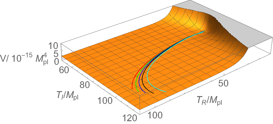
7 Discussion

7.1 The scale of the potential

Referring to Figure 1 and 7, one can see that the evolution paths exist at different energy scales. In fact, there are two main parameters affecting the potential scale. One is $\left|{\mu}\right|$, and another is ${\rho}$. Referring to Eq.(49), (50) and (51), one can see that the potential is directly proportional to $\left|{\mu}\right|^{2}$, while the powers of $\left(\frac{{M}_{\text{pl}}}{2{T}_{R}}\right)^{\rho}$ in Eq.(49), $\left(\frac{\left({\rho}^{2}-7\rho+4\right){M}_{\text{pl}}}{-\left(\rho-3\right)\rho{\iota}_{1}}\right)^{\rho-1}$ in Eq.(50) and $\left(\frac{\left({\rho}^{2}-7\rho+4\right){M}_{\text{pl}}}{-\left(\rho-3\right)\rho{\iota}_{1}}\right)^{\rho-1}$ in Eq.(51) show ${\rho}$ is related to the power of some field values and parameters. Since $\left|{\mu}\right|$ is held in a fixed scale $O\left({10}^{-4}\right){M}_{\text{pl}}$, the difference lies in various ${\rho}$. Since the scale of field values is $O\left({10}^{2}\right){M}_{\text{pl}}$, the potential scale decreases by ${10}^{-2}$ times as ${\rho}$ increases by $1$.

7.2 Turn rate for ${\rho}\neq 3$

In Figure 2 and 8, one can see that there are path patterns with various extent of turning. This can be tracked by Figure 5 (and 11) respectively. For example, for ${\omega}_{1}>0$ and ${\rho}=4$, when the background fields roll off from the initial point, there is no rigorous turning until the end of inflation, leading to the evolution of $2\omega/H$ close to zero. As they gradually approach to their corresponding minimum points, Hubble scale $H$ reduces gradually and the turning becomes rigorous, resulting in the gradual rise of $2\omega/H$. Finally, when they oscillate around their minimum points, the turning becomes sharply rigorous, leading to the sudden surge of $2\omega/H$. Similar arguments can also be made for other cases by tracking the evolution paths and the variations of $2\omega/H$.

7.3 The turning for ${\rho}=3$ and the afterward evolution

From Figure 18, since the initial speeds of background fields have the small scale ${10}^{-5}{M}_{\text{pl}}$, it is not obvious to see the turning. Hence, we demonstrate the inflation path with the greatest possible initial speed of ${T}_{I}$. The parameter sets are shown in Table 12 and their corresponding evolution paths are shown in Figure 19. We can significantly see that the background fields move along ${T}_{I}$ a little while and turn towards the decreasing ${T}_{R}$ direction. However, ${\alpha}\left(N\right)$ is reduced as the initial speed of background fields increases. That is because the turn rate per Hubble parameter is mainly inversely proportional to the resultant field rate. Hence, even though it is not significant to see the turning in the field evolution graph, the initial ${\alpha}\left(N\right)$ is comparatively large, and vice versa. After that, the background fields keep its ${T}_{I}$ coordinate when they continue rolling. This is because Hubble parameter and $\dot{T}_{R}/{T}_{R}$ in Eq.(63) act as friction terms to stabilize the curve at a constant ${T}_{I}$ coordinate.

Color	$\left|{\mu}\right|/{M}_{\text{pl}}^{2}$	${\iota}_{1}/{M}_{\text{pl}}$	${M}_{3/2+}/{M}_{\text{pl}}$	${T}_{R\text{end}}/{M}_{\text{pl}}$	${T}_{R\text{hc}}/{M}_{\text{pl}}$	${T}_{I\text{hc}}/{M}_{\text{pl}}$	${N}_{\text{end}}$	${N}_{\text{stop}}$	${\beta}_{\text{iso}}$	$\cos{\left(\Delta\right)}$
Gray	${10}^{-4}$	$-2$	$1.36083\times{10}^{-5}$	$3$	$225$	$80$	$53.7825$	$54.1041$	$7.54744\times{10}^{-36}$	$3.28888\times{10}^{-6}$
Magenta	${10}^{-4}$	$-2.5$	$1.21716\times{10}^{-5}$	$3.75$	$280$	$80$	$53.5343$	$53.8559$	$1.36149\times{10}^{-34}$	$2.63095\times{10}^{-5}$
Brown	${10}^{-4}$	$-3$	$1.11111\times{10}^{-5}$	$4.5$	$340$	$80$	$54.1961$	$54.5177$	$1.68237\times{10}^{-37}$	$2.19281\times{10}^{-6}$
Orange	${10}^{-4}$	$-4$	$9.6225\times{10}^{-6}$	$6$	$450$	$80$	$53.7825$	$54.1041$	$2.19583\times{10}^{-35}$	$1.64444\times{10}^{-6}$
Pink	${10}^{-4}$	$-5$	$8.60663\times{10}^{-6}$	$7.5$	$600$	$80$	$57.5058$	$57.8274$	$7.62281\times{10}^{-36}$	$1.31667\times{10}^{-6}$
Red	${10}^{-4}$	$-1$	$1.9245\times{10}^{-5}$	$1.5$	$105$	$20$	$50.061$	$50.3826$	$7.23759\times{10}^{-34}$	$6.57141\times{10}^{-6}$
Green	${10}^{-4}$	$-1$	$1.9245\times{10}^{-5}$	$1.5$	$110$	$20$	$52.5417$	$52.9298$	$5.27718\times{10}^{-32}$	$6.57574\times{10}^{-6}$
Blue	${10}^{-4}$	$-1$	$1.9245\times{10}^{-5}$	$1.5$	$115$	$20$	$55.0234$	$55.3450$	$8.40563\times{10}^{-35}$	$6.57969\times{10}^{-6}$
Black	${10}^{-4}$	$-1$	$1.9245\times{10}^{-5}$	$1.5$	$120$	$20$	$57.5058$	$57.8274$	$1.87223\times{10}^{-35}$	$6.58331\times{10}^{-6}$
Cyan	${10}^{-4}$	$-1$	$1.9245\times{10}^{-5}$	$1.5$	$123$	$20$	$58.9956$	$59.3172$	$2.43366\times{10}^{-33}$	$6.58534\times{10}^{-6}$

Table 11: Feasible parameter sets for inflation for ${\rho}=3$. In these sets, ${T^{\prime}}_{R\text{hc}}={T^{\prime}}_{I\text{hc}}={10}^{-5}{M}_{\text{pl}}$. ${N}_{\text{end}}$ is the e-folding number when ${\epsilon}=1$, which represents the end of inflation. ${N}_{\text{stop}}$ means the e-folding number that we stop the numerical calculation.

Color	$\left|{\mu}\right|/{M}_{\text{pl}}^{2}$	${\iota}_{1}/{M}_{\text{pl}}$	${T}_{R\text{end}}/{M}_{\text{pl}}$	${T}_{R\text{hc}}/{M}_{\text{pl}}$	${T}_{I\text{hc}}/{M}_{\text{pl}}$	${T^{\prime}}_{R\text{hc}}/{M}_{\text{pl}}$	${T^{\prime}}_{I\text{hc}}/{M}_{\text{pl}}$	${N}_{\text{end}}$	${N}_{\text{stop}}$	${\beta}_{\text{iso}}$	$\cos{\left(\Delta\right)}$
Cyan	${10}^{-4}$	$-1$	$1.5$	$105$	$60$	${10}^{-5}$	${10}^{-3}$	$50.061$	$50.3826$	$9.20002\times{10}^{-36}$	$3.28604\times{10}^{-4}$
Black	${10}^{-4}$	$-1$	$1.5$	$105$	$50$	${10}^{-5}$	${10}^{-2}$	$50.061$	$50.3826$	$1.82773\times{10}^{-30}$	$3.2857\times{10}^{-3}$
Blue	${10}^{-4}$	$-1$	$1.5$	$105$	$40$	${10}^{-5}$	${10}^{-1}$	$50.061$	$50.3826$	$4.48765\times{10}^{-39}$	$3.28483\times{10}^{-2}$
Green	${10}^{-4}$	$-1$	$1.5$	$105$	$30$	${10}^{-5}$	$1$	$50.0607$	$50.3823$	$1.87863\times{10}^{-9}$	$3.203\times{10}^{-1}$
Red	${10}^{-4}$	$-1$	$1.5$	$105$	$20$	${10}^{-5}$	$2$	$50.0599$	$50.3815$	$6.73078\times{10}^{-7}$	$5.7951\times{10}^{-1}$

Table 12: Parameter sets for showing the significant turning in ${\rho}=3$ case. The difference of each parameter sets lie in ${T^{\prime}}_{I\text{hc}}/{M}_{\text{pl}}$, the initial rate of ${T}_{I}$ and the initial coordinate of ${T}_{I}$. ${N}_{\text{end}}$ is the e-folding number when ${\epsilon}=1$, which represents the end of inflation. ${N}_{\text{stop}}$ means the e-folding number that we stop the numerical calculation.

Figure 18: Left: Evolutions of $\left({\mu}_{s}/H\right)^{2}$ for ${{\rho}}=3$. Right: A close shot from $0$ to $4$ e-foldings. Various colors refer to various parameter sets listed on Table 12.

7.4 The smallness of ${\beta}_{\text{iso}}$ and $\cos{\left({\Delta}\right)}$

To understand the smallness of ${\beta}_{\text{iso}}$ and $\cos{\left({\Delta}\right)}$, we should consider the reason of smallness of ${T}_{\mathcal{SS}}$ and ${T}_{\mathcal{RS}}$, since they are related by Eq.(64) and (65). By Eq.(118) and (119) (or by Eq.(116) and (117)), we can see that ${T}_{\mathcal{SS}}$ and ${T}_{\mathcal{RS}}$ depend on the strengths of ${\alpha}$ (turn rate per Hubble parameter) and ${\beta}$. By Figure 5, 6, 11 and 12, we can see ${\alpha}\left(N\right)$ is nearly zero, while ${\beta}\left(N\right)$ keeps negative from ${N}_{\text{hc}}$ to ${N}_{\text{end}}$. These show that ${T}_{\mathcal{SS}}$ becomes exponentially suppressed and there is very small contribution by each $dN$ in the integration of ${T}_{\mathcal{RS}}$, leading to smallness of ${T}_{\mathcal{SS}}$ and ${T}_{\mathcal{RS}}$, and so are ${\beta}_{\text{iso}}$ and $\cos{\left({\Delta}\right)}$.

Figure 19: Field evolution at different $\alpha\left(N\right)$ (Left) and their corresponding initial turn rate per Hubble parameter (Right). Here, the field value ${T}_{I}$ does not affect the strength of $\alpha\left(N\right)$. Thus, for obvious observation, we evaluate at different ${T}_{I}$. Various colors refer to various parameter sets listed on Table 12.

8 Conclusion

We studied the inflation dynamics of generalized dilaton-axion models with a new Fayet-Iliopoulos (FI) term not requiring gauging R-symmetry, where both dilaton ${T}_{R}$ and its axionic partner ${T}_{I}$ are responsible for contributing the evolution of inflation. We found that to obtain dS vacuum at the end of inflation, integer ${\rho}$ in the generalized Kähler potential is constrained at different cases of ${\omega}_{1}$. Particularly, when ${\rho}=3$, the axionic partner does not contribute to the inflation as it is absent in the total potential. We also evaluated the feasible initial conditions to produce successful inflation based on Planck observation and e-folding constraint and showed different evolution paths with various turning patterns of the background field. This shows that apart from slow roll parameters, spectral index and inflation energy scale, the change of turn rates can also be one of the fingerprints to identify the specific inflation pattern in double field model verification. Finally, we gave the predictions of iso-curvature mode contributions such as ${\beta}_{\text{iso}}$ and $\cos{\Delta}$.

9 Acknowledgement

The author thanks Prof. Hiroyuki ABE very much for suggestion and useful discussions. The author is supported by AY 2019 Scholarship for Young Doctoral Students, Waseda University.

Appendix A Christoffel symbols and curvatures of field spaces

Given that the metric of the field space in the Einstein frame is given by

$$\mathcal{G}_{IJ}=\frac{{\rho}{M}_{\text{pl}}^{2}}{2{T}_{R}^{2}}{\delta}_{IJ}\quad\forall\;I,J\in\left\{1,2\right\},\\$$ (66)

the non-zero Christoffel symbols defined by

$${\Gamma}^{I}_{JK}=\frac{1}{2}\mathcal{G}^{IL}\left(\mathcal{G}_{LJ,K}+\mathcal{G}_{LK,J}-\mathcal{G}_{JK,L}\right),\\$$ (67)

are

$$-{\Gamma}^{1}_{11}={\Gamma}^{1}_{22}=-{\Gamma}^{2}_{12}=-{\Gamma}^{2}_{21}=\frac{1}{{T}_{R}}.\\$$ (68)

The non-zero curvature tensors defined by

$${R}^{I}_{JKL}={\partial}_{K}{\Gamma}^{I}_{JL}+{\Gamma}^{I}_{CK}{\Gamma}^{C}_{JL}-\left({\partial}_{L}{\Gamma}^{I}_{JK}+{\Gamma}^{I}_{CL}{\Gamma}^{C}_{JK}\right),\\$$ (69)

are

$$-{R}^{1}_{212}={R}^{1}_{221}={R}^{2}_{112}=-{R}^{2}_{121}=\frac{1}{{T}_{R}^{2}},\\$$ (70)

which gives the Ricci tensor defined by ${R}_{JL}=\mathcal{G}^{K}_{I}{R}^{I}_{JKL}={R}^{I}_{JIL}$ as

$${R}_{11}={R}_{22}=-\frac{1}{{T}_{R}^{2}},\\$$ (71)

and the curvature scalar, defined by $R\equiv\mathcal{G}^{IJ}{R}_{IJ}$, as

$$R=-\frac{4}{{\rho}{M}_{\text{pl}}^{2}}.\\$$ (72)

Appendix B A formalism of Double Field Inflation

In this section, we follow the derivation in [6] and [9]. Note that in the Jordan frame, the Lagrangian is

$${S}_{\text{Jordan}}=\int d^{4}x\sqrt{-\tilde{g}}\left[f\left({\phi}^{I}\right)\tilde{R}-\frac{1}{2}\tilde{\mathcal{G}}_{IJ}\tilde{g}^{{\mu}{\nu}}\tilde{\triangledown}_{\mu}{\phi}^{I}\tilde{\triangledown}_{\nu}{\phi}^{J}-\tilde{V}\left({\phi}^{I}\right)\right].\\$$ (73)

where $f\left({\phi}^{I}\right)$ is the non-minimal coupling function and $\tilde{V}\left({\phi}^{I}\right)$ is the potential for the scalar fields in the Jordan frame. To change the equation in Jordan frame into the counterpart in Einstein frame, we define a spacetime metric in the Einstein frame ${g}_{{\mu}{\nu}}\left(x\right)$ as

$${g}_{{\mu}{\nu}}\left(x\right)={\Omega}^{2}\left(x\right)\tilde{g}_{{\mu}{\nu}}\left(x\right),\\$$ (74)

where the conformal factor ${\Omega}^{2}\left(x\right)$ is given by

$${\Omega}^{2}\left(x\right)=\frac{2}{{M}^{2}_{\text{pl}}}f\left({\phi}^{I}\left(x\right)\right).\\$$ (75)

Then, the action in Jordan frame becomes that in Einstein frame, which is given by

$${S}_{\text{Einstein}}=\int d^{4}x\sqrt{-{g}}\left[\frac{{M}^{2}_{\text{pl}}}{2}{R}-\frac{1}{2}{\mathcal{G}}_{IJ}{g}^{{\mu}{\nu}}{\triangledown}_{\mu}{\phi}^{I}{\triangledown}_{\nu}{\phi}^{J}-{V}\left({\phi}^{I}\right)\right].\\$$ (76)

and the potential in the Einstein frame becomes

$$V\left({\phi}^{I}\right)=\frac{\tilde{V}\left({\phi}^{I}\right)}{{\Omega}^{4}\left(x\right)}=\frac{{M}^{4}_{\text{pl}}}{4f^{2}\left({\phi}^{I}\right)}\tilde{V}\left({\phi}^{I}\right).\\$$ (77)

The coefficients $\mathcal{G}_{{I}{J}}$ of the non-canonical kinetic terms in the Einstein frame depend on the non-minimal coupling function $f\left({\phi}^{I}\right)$ and its derivatives. They are given by

$$\mathcal{G}_{{I}{J}}\left({\phi}^{K}\right)=\frac{{M}^{2}_{\text{pl}}}{2f\left({\phi}^{L}\right)}\left[\tilde{\mathcal{G}}_{{I}{J}}\left({\phi}^{K}\right)+\frac{3}{f\left({\phi}^{L}\right)}{f}_{,I}{f}_{,J}\right],\\$$ (78)

where ${f}_{,I}=\frac{{\partial}{f}}{{\partial}{\phi}^{I}}$. Varying the action in Einstein frame with respect to ${g}_{{\mu}{\nu}}\left(x\right)$, we have the Einstein equations

$${R}_{{\mu}{\nu}}-\frac{1}{2}{g}_{{\mu}{\nu}}R=\frac{1}{{M}^{2}_{\text{pl}}}{T}_{{\mu}{\nu}},\\$$ (79)

where

$${T}_{{\mu}{\nu}}=\mathcal{G}_{{I}{J}}{\partial}_{\mu}{\phi}^{I}{\partial}_{\nu}{\phi}^{J}-{g}_{{\mu}{\nu}}\left[\frac{1}{2}\mathcal{G}_{{K}{L}}{\partial}_{\gamma}{\phi}^{K}{\partial}^{\gamma}{\phi}^{L}+V\left({\phi}^{K}\right)\right].\\$$ (80)

Varying Eq. (77) with respect to ${\phi}^{I}$, we obtain the equation of motion for ${\phi}^{I}$

$$\square{\phi}^{I}+{g}^{{\mu}{\nu}}{\Gamma}^{I}_{{J}{K}}{\partial}_{\mu}{\phi}^{J}{\partial}_{\nu}{\phi}^{K}-\mathcal{G}^{{I}{K}}{V}_{,K}=0,\\$$ (81)

where $\square{\phi}^{I}={g}^{{\mu}{\nu}}{\phi}^{I}_{;{\mu}{\nu}}$ and ${\Gamma}^{I}_{{J}{K}}$ is the Christoffel symbol for the field space manifold in terms of $\mathcal{G}_{{I}{J}}$ and its derivative. Expanding each scalar field to the first order around its classical background value,

$${\phi}^{I}\left({x}^{\mu}\right)={\varphi}^{I}\left(t\right)+{\delta}{\phi}^{I}\left({x}^{\mu}\right),\\$$ (82)

and perturbing a spatially flat Friedmann-Robertson-Walker (FRW) metric,

$$ds^{2}={g}_{{\mu}{\nu}}d{x}^{\mu}d{x}^{\nu}=-\left(1+2A\right)dt^{2}+2a\left({\partial}_{i}B\right)d{x}^{i}dt+a^{2}\left[\left(1-2{\psi}\right){\delta}_{ij}+2{\partial}_{i}{\partial}_{j}E\right]d{x}^{i}d{x}^{j},\\$$ (83)

where $a\left(t\right)$ is the scale factor. To the zeroth order, the $00$ and $ij$ components of the Einstein equations become

$$H^{2}=\frac{1}{3{M}^{2}_{\text{pl}}}\left[\frac{1}{2}\mathcal{G}_{{I}{J}}\dot{\varphi}^{I}\dot{\varphi}^{J}+V\left({\varphi}^{I}\right)\right],\\$$ (84)

$$\dot{H}=-\frac{1}{2{M}^{2}_{\text{pl}}}\mathcal{G}_{{I}{J}}\dot{\varphi}^{I}\dot{\varphi}^{J},\\$$ (85)

where $H=\frac{\dot{a}\left(t\right)}{a\left(t\right)}$ is the Hubble parameter, and the field field space metric is calculated at the zeroth order, $\mathcal{G}_{{I}{J}}=\mathcal{G}_{{I}{J}}\left({\varphi}^{K}\right)$. Introducing the number of e-folding $N=\ln{a}$ with $dN=Hdt$, the above Einstein equation becomes

$$3{M}^{2}_{\text{pl}}-\frac{1}{2}\mathcal{G}_{{I}{J}}{{\varphi}^{I}}^{\prime}{{\varphi}^{J}}^{\prime}=\frac{V\left({\varphi}^{I}\right)}{H^{2}},\\$$ (86)

$$\frac{H^{\prime}}{H}=-\frac{1}{2{M}^{2}_{\text{pl}}}\mathcal{G}_{{I}{J}}{{\varphi}^{I}}^{\prime}{{\varphi}^{J}}^{\prime},\\$$ (87)

where the prime ^′ means the derivative with respect to $N$. For any vector in the field space $A^{I}$, we define a covariant derivative with respect to the field-space metric as usual by

$$\mathcal{D}_{J}{A}^{I}={\partial}_{J}{A}^{I}+{\Gamma}^{I}_{{J}{K}}{A}^{K},\\$$ (88)

and the time derivative with respect to the cosmic time $t$ is given by

$$\mathcal{D}_{t}{A}^{I}\equiv\dot{\varphi}^{J}\mathcal{D}_{J}{A}^{I}=\dot{A}^{I}+{\Gamma}^{I}_{{J}{K}}\dot{\varphi}^{J}{A}^{K}=H\left({{A}^{I}}^{\prime}+{\Gamma}^{I}_{{J}{K}}{{\varphi}^{J}}^{\prime}{A}^{K}\right).\\$$ (89)

Now, we define the length of the velocity vector for the background fields as

$$|\dot{\varphi}^{I}|\equiv\dot{\sigma}=\sqrt{\mathcal{G}_{{P}{Q}}\dot{\varphi}^{P}\dot{\varphi}^{Q}}\quad\Rightarrow\quad|{{\varphi}^{I}}^{\prime}|\equiv{\sigma}^{\prime}=\sqrt{\mathcal{G}_{{P}{Q}}{{\varphi}^{P}}^{\prime}{{\varphi}^{Q}}^{\prime}}.$$ (90)

Introducing the unit vector of the velocity vector of the background fields

$$\hat{\sigma}^{I}\equiv\frac{\dot{\varphi}^{I}}{\dot{\sigma}}=\frac{{{\varphi}^{I}}^{\prime}}{{\sigma}^{\prime}}=\frac{{{\varphi}^{I}}^{\prime}}{\sqrt{\mathcal{G}_{{P}{Q}}{{\varphi}^{P}}^{\prime}{{\varphi}^{Q}}^{\prime}}}$$ (91)

the $00$ and $ij$ components of the Einstein equations become

$$H^{2}=\frac{1}{3{M}^{2}_{\text{pl}}}\left[\frac{1}{2}\dot{\sigma}^{2}+V\right]\quad\Leftrightarrow\quad 3{M}^{2}_{\text{pl}}-\frac{1}{2}{{\sigma}^{\prime}}^{2}=\frac{V\left({\varphi}^{I}\right)}{H^{2}}\quad\Leftrightarrow\quad\frac{V}{{M}_{\text{pl}}^{2}H^{2}}=\left(3-{\epsilon}\right),\\$$ (92)

$$\dot{H}=-\frac{1}{2{M}^{2}_{\text{pl}}}\dot{\sigma}^{2}\quad\Leftrightarrow\quad\frac{H^{\prime}}{H}=-\frac{1}{2{M}^{2}_{\text{pl}}}{{\sigma}^{\prime}}^{2}\quad\Leftrightarrow\quad\frac{\dot{\sigma}^{2}}{{M}_{\text{pl}}^{2}H^{2}}=2{\epsilon},\\$$ (93)

and the equation of motion of ${\phi}^{I}$ in the zeroth order is

$$\ddot{\sigma}+3H\dot{\sigma}+{V}_{,\sigma}=0\quad\Leftrightarrow\quad\frac{\ddot{\sigma}}{H\dot{\sigma}}=-3-\frac{3-{\epsilon}}{2{\epsilon}}\frac{d}{dN}\left(\ln{V}\right),\\$$ (94)

where

$${V}_{,\sigma}\equiv\hat{\sigma}^{I}{V}_{,I}.\\$$ (95)

and ${\epsilon}$ is the first order Hubble slow-roll parameter defined in Eq.(98). Now, we define a quantity $\hat{s}^{{I}{J}}$ to obtain the field component orthogonal to $\hat{\sigma}^{I}$

$$\hat{s}^{{I}{J}}\equiv\mathcal{G}^{{I}{J}}-\hat{\sigma}^{I}\hat{\sigma}^{J},\\$$ (96)

which obeys the following relations with $\hat{\sigma}^{I}$

$$\begin{split}\hat{\sigma}_{I}\hat{\sigma}^{I}=1,\\ \hat{s}^{{I}{J}}\hat{s}_{{I}{J}}=\mathcal{N}-1,\\ \hat{s}^{I}_{\;A}\hat{s}^{A}_{\;J}=\hat{s}^{I}_{\;J},\\ \hat{\sigma}_{I}\hat{s}^{{I}{J}}=0\quad\forall J.\\ \end{split}$$ (97)

The slow-roll parameters are given by

$$\epsilon\equiv-\frac{\dot{H}}{H^{2}}=\frac{3\dot{\sigma}^{2}}{\dot{\sigma}^{2}+2V}\quad\Leftrightarrow\quad\frac{\dot{\sigma}^{2}}{V}=\frac{2{\epsilon}}{3-{\epsilon}},\\$$ (98)

and

$${\eta}_{{\sigma}{\sigma}}\equiv{M}^{2}_{\text{pl}}\frac{\mathcal{M}_{{\sigma}{\sigma}}}{V}\quad\text{and}\quad{\eta}_{{s}{s}}\equiv{M}^{2}_{\text{pl}}\frac{\mathcal{M}_{{s}{s}}}{V},\\$$ (99)

where $\mathcal{M}^{I}_{J}$ is the effective mass squared matrix given by

$$\begin{split}{\mathcal{M}}^{I}_{J}\equiv&\;\mathcal{G}^{IK}\left(\mathcal{D}_{J}\mathcal{D}_{K}V\right)-\mathcal{R}^{I}_{LMJ}\dot{\varphi}^{L}\dot{\varphi}^{M},\\ {\mathcal{M}}_{{\sigma}{J}}\equiv&\;\hat{\sigma}_{I}\mathcal{M}^{I}_{J}=\hat{\sigma}^{K}\left(\mathcal{D}_{K}\mathcal{D}_{J}V\right),\\ {\mathcal{M}}_{{\sigma}{\sigma}}\equiv&\;\hat{\sigma}_{I}\hat{\sigma}^{J}\mathcal{M}^{I}_{J}=\hat{\sigma}^{K}\hat{\sigma}^{J}\left(\mathcal{D}_{K}\mathcal{D}_{J}V\right),\\ {\mathcal{M}}_{{s}{J}}\equiv&\;\hat{s}_{I}\mathcal{M}^{I}_{J}=\hat{s}_{I}\left(\mathcal{G}^{IK}\left(\mathcal{D}_{J}\mathcal{D}_{K}V\right)-\mathcal{R}^{I}_{LMJ}\dot{\varphi}^{L}\dot{\varphi}^{M}\right),\\ {\mathcal{M}}_{{s}{s}}\equiv&\;\hat{s}_{I}\hat{s}^{J}\mathcal{M}^{I}_{J}=\hat{s}_{I}\hat{s}^{J}\left(\mathcal{G}^{IK}\left(\mathcal{D}_{J}\mathcal{D}_{K}V\right)-\mathcal{R}^{I}_{LMJ}\dot{\varphi}^{L}\dot{\varphi}^{M}\right),\\ \end{split}$$ (100)

and $\hat{s}^{I}$ is defined in the following argument. Now we define the turn-rate vector ${\omega}^{I}$ as the covariant rate of change of the unit vector $\hat{\sigma}^{I}$

$${\omega}^{I}\equiv\mathcal{D}_{t}\hat{\sigma}^{I}=-\frac{1}{\dot{\sigma}}{V}_{,K}\hat{s}^{{I}{K}}=\frac{-1}{H{\sigma}^{\prime}}{V}_{,K}\hat{s}^{{I}{K}}.\\$$ (101)

Since ${\omega}^{I}\propto\hat{s}^{{I}{K}}$, we have

$${\omega}^{I}\hat{\sigma}_{I}=0.\\$$ (102)

We can also find

$$\mathcal{D}_{t}\hat{s}^{{I}{J}}=-\hat{\sigma}^{I}{\omega}^{J}-\hat{\sigma}^{J}{\omega}^{I}.\\$$ (103)

Also, we introduce a new unit vector $\hat{s}^{I}$ pointing in the direction of the turn-rate, ${\omega}^{I}$, and a new projection operator ${\gamma}^{{I}{J}}$

$$\hat{s}^{I}\equiv\frac{{\omega}^{I}}{\omega},\\$$ (104)

$${\gamma}^{{I}{J}}\equiv{\mathcal{G}}^{{I}{J}}-\hat{\sigma}^{I}\hat{\sigma}^{J}-\hat{s}^{I}\hat{s}^{J}.\\$$ (105)

where ${\omega}=|{\omega}^{I}|$ is the magnitude of the turn-rate vector. The new unit vector $\hat{s}^{I}$ and the new projection operator ${\gamma}^{{I}{J}}$ also satisfy

$$\begin{split}\hat{s}^{{I}{J}}=&\hat{s}^{I}\hat{s}^{J}+{\gamma}^{{I}{J}},\\ {\gamma}^{{I}{J}}{\gamma}_{{I}{J}}=&\mathcal{N}-2,\\ \hat{s}^{{I}{J}}\hat{s}_{J}=&\hat{s}^{I},\\ \hat{\sigma}_{I}\hat{s}^{I}=&\hat{\sigma}_{I}{\gamma}^{{I}{J}}=\hat{s}_{I}{\gamma}^{{I}{J}}=0\quad\forall J.\end{split}$$ (106)

We then find

$${\mathcal{D}}_{t}\hat{s}^{I}=-{\omega}\hat{\sigma}^{I}-{\Pi}^{I},\\ {\mathcal{D}}_{t}{\gamma}^{{I}{J}}=\hat{s}^{I}{\gamma}^{J}+\hat{s}^{J}{\gamma}^{I},\\$$ (107)

where

$${\Pi}^{I}\equiv\frac{1}{\omega}{\mathcal{M}}_{{\sigma}{K}}{\gamma}^{{I}{K}},\\$$ (108)

and hence

$$\hat{\sigma}_{I}{\Pi}^{I}=\hat{s}_{I}{\Pi}^{I}=0,\\$$ (109)

Now, we define the curvature and entropic perturbations as follows

$$\mathcal{R}={\psi}+\frac{H}{\dot{\sigma}}\hat{\sigma}_{J}{\delta}{\phi}^{J}=\frac{H}{\dot{\sigma}}{Q}_{\sigma},\\$$ (110)

$$\mathcal{S}=\frac{H}{\dot{\sigma}}{Q}_{s},\\$$ (111)

whose E.O.M.s are given by [9]

$$\begin{split}\ddot{Q}_{\sigma}+3H\dot{Q}_{\sigma}+\left[\left(\frac{k}{a}\right)^{2}+\mathcal{M}_{{\sigma}{\sigma}}-{\omega}^{2}-\frac{1}{{M}_{\text{pl}}^{2}a^{3}}\frac{d}{dt}\left(\frac{a^{3}\dot{\sigma}^{2}}{H}\right)\right]{Q}_{\sigma}=&\;2\frac{d}{dt}\left({\omega}{Q}_{s}\right)-2\left(\frac{{V}_{,\sigma}}{\dot{\sigma}}+\frac{\dot{H}}{H}\right){\omega}{Q}_{s},\\ \ddot{Q}_{s}+3H\dot{Q}_{s}+\left[\left(\frac{k}{a}\right)^{2}+\mathcal{M}_{ss}+3{\omega}^{2}\right]{Q}_{s}=&\;4{M}_{\text{pl}}^{2}\frac{\omega}{\dot{\sigma}}\frac{k^{2}}{a^{2}}{\Psi},\\ \end{split}$$ (112)

where $\Psi$ is the gauge-invariant Bardeen potential [7, 8], $\mathcal{M}_{{\sigma}{\sigma}}$ and $\mathcal{M}_{ss}$ are given by Eq.(100) and

$${\mu}_{s}^{2}=\mathcal{M}_{ss}+3{\omega}^{2},\\$$ (113)

is an effective square mass of entropy perturbations. After the first horizon crossing, the co-moving wave number $k$ obeys $\frac{k}{aH}<1$. Hence, the curvature and entropic perturbations satisfy the following equations

$$\dot{\mathcal{R}}={\alpha}H\mathcal{S}+O\left(\frac{k^{2}}{a^{2}H^{2}}\right),\\$$ (114)

$$\dot{\mathcal{S}}={\beta}H\mathcal{S}+O\left(\frac{k^{2}}{a^{2}H^{2}}\right),\\$$ (115)

which allows us to write the transfer functions

$${T}_{\mathcal{RS}}\left({t}_{\text{hc}},t\right)=\int^{t}_{{t}_{\text{hc}}}d{t}^{\prime}{\alpha}\left(t^{\prime}\right)H\left(t^{\prime}\right){T}_{\mathcal{SS}}\left({t}_{\text{hc}},t^{\prime}\right),\\$$ (116)

$${T}_{\mathcal{SS}}\left({t}_{\text{hc}},t\right)=\exp\left[\int^{t}_{{t}_{\text{hc}}}{dt^{\prime}}{\beta}\left(t^{\prime}\right)H\left(t^{\prime}\right)\right].\\$$ (117)

where ${t}_{\text{hc}}$ is the time of the first horizon crossing. Being changed from the cosmic time $t$ into the number of e-folding $N=\ln{a}$, where $dN=Hdt$, ${T}_{\mathcal{RS}}\left({t}_{\text{hc}},t\right)$ and ${T}_{\mathcal{SS}}\left({t}_{\text{hc}},t\right)$ become

$${T}_{\mathcal{RS}}\left({N}_{\text{hc}},N\right)=\int^{N}_{{N}_{\text{hc}}}{dN^{\prime}}{\alpha}\left(N^{\prime}\right){T}_{\mathcal{SS}}\left({N}_{\text{hc}},N^{\prime}\right),\\$$ (118)

and

$${T}_{\mathcal{SS}}\left({N}_{\text{hc}},N\right)=\exp\left[\int^{N}_{{N}_{\text{hc}}}{dN^{\prime}}{\beta}\left(N^{\prime}\right)\right].\\$$ (119)

Now that the E.O.M.s of curvature and entropic perturbations are [6]

$$\dot{\mathcal{R}}=2{\omega}\mathcal{S}+O\left(\frac{k^{2}}{a^{2}H^{2}}\right),\\$$ (120)

and

$$\dot{Q}_{s}\simeq-\frac{{\mu}^{2}_{s}}{3H}{Q}_{s},\\$$ (121)

where the effective squared mass of the entropy perturbation can be written as that relative to the Hubble scale as

$${\mu}^{2}_{s}={\mathcal{M}}_{ss}+3{\omega}^{2}\quad\Leftrightarrow\quad\frac{{\mu}^{2}_{s}}{H^{2}}=\left(3-{\epsilon}\right){\eta}_{ss}+\frac{3}{4}{\alpha}^{2},\\$$ (122)

and $\simeq$ means slow-roll approximation and ${\alpha}$ is given in Eq.(123). Comparing with Eq.(110), (111), (114) and (115) with Eq.(120) and (121) [6], we obtain

$${\alpha}\left(t\right)=\frac{2{\omega}\left(t\right)}{H\left(t\right)}\quad\Leftrightarrow\quad{\alpha}\left(N\right)=\frac{2{\omega}\left(N\right)}{H\left(N\right)},\\$$ (123)

and

$${\beta}=-\frac{{\mu}^{2}_{s}}{3H^{2}}-{\epsilon}-\frac{\ddot{\sigma}}{H\dot{\sigma}}=-{\eta}_{ss}\left(1-\frac{1}{3}{\epsilon}\right)+\left(3-{\epsilon}\right)+\frac{3-{\epsilon}}{2{\epsilon}}\frac{d}{dN}\left({\ln{V}}\right)-\frac{1}{4}{\alpha}^{2},\\$$ (124)

Note that the power spectrum for the gauge invariant curvature perturbation is given by

$$\langle\mathcal{R}\left(\mathbb{k}_{1}\right)\mathcal{R}\left(\mathbb{k}_{2}\right)\rangle=\left(2\pi\right)^{3}{\delta}^{\left(3\right)}\left(\mathbb{k}_{1}+\mathbb{k}_{2}\right){P}_{\mathcal{R}}\left({k}_{1}\right),\\$$ (125)

where ${P}_{\mathcal{R}}\left(k\right)=|\mathcal{R}|^{2}$. The dimensionless power spectrum is

$${\mathcal{P}}_{\mathcal{R}}=\frac{k^{3}}{2{\pi}^{2}}|\mathcal{R}|^{2},\\$$ (126)

and the spectral index is defined as

$${n}_{s}\equiv 1+\frac{d\ln{\mathcal{P}}_{\mathcal{R}}}{d\ln{k}_{\text{hc}}},\\$$ (127)

where ${k}_{\text{hc}}=a\left({t}_{\text{hc}}\right)H\left({t}_{\text{hc}}\right)$ represents the pivot scale at the first horizon crossing ${t}_{\text{hc}}$, which is related to the cosmic time $t$ by

$$\frac{d\ln{k}}{dt}=\frac{d\left(aH\right)}{dt}=\frac{\dot{a}}{a}+\frac{\dot{H}}{H}=H\left(1+\frac{\dot{H}}{H^{2}}\right)=\left(1-{\epsilon}\right)H.\\$$ (128)

Using the transfer function, we can relate the power spectra of adiabatic and entropic perturbations at time ${t}_{\text{hc}}$ to its value at some later time $t>{t}_{\text{hc}}$ with the corresponding pivot scale $k$ as

$$\begin{split}{\mathcal{P}}_{\mathcal{R}}\left(k\right)=&\;{\mathcal{P}}_{\mathcal{R}}\left({k}_{\text{hc}}\right)\left[1+{T}^{2}_{\mathcal{RS}}\left({t}_{\text{hc}},t\right)\right],\\ {\mathcal{P}}_{\mathcal{S}}\left(k\right)=&\;{\mathcal{P}}_{\mathcal{R}}\left({k}_{\text{hc}}\right){T}^{2}_{\mathcal{SS}}\left({t}_{\text{hc}},t\right),\\ \end{split}$$ (129)

The transfer functions are given by

$$\begin{split}\frac{1}{H\left({t}_{\text{hc}}\right)}\frac{{\partial}{T}_{\mathcal{RS}}\left({t}_{\text{hc}},t\right)}{{\partial}{t}_{\text{hc}}}&=\;-{\alpha}\left({t}_{\text{hc}}\right)-{\beta}\left({t}_{\text{hc}}\right){T}_{\mathcal{SS}}\left({t}_{\text{hc}},{t}\right),\\ \frac{1}{H\left({t}_{\text{hc}}\right)}\frac{{\partial}{T}_{\mathcal{SS}}\left({t}_{\text{hc}},t\right)}{{\partial}{t}_{\text{hc}}}&=\;-{\beta}\left({t}_{\text{hc}}\right){T}_{\mathcal{SS}}\left({t}_{\text{hc}},t\right).\\ \end{split}$$ (130)

In term of the number of e-folding $N$, the above differential equation becomes

$$\begin{split}\frac{{\partial}{T}_{\mathcal{RS}}\left({N}_{\text{hc}},N\right)}{{\partial}{N}_{\text{hc}}}&=\;-{\alpha}\left({N}_{\text{hc}}\right)-{\beta}\left({N}_{\text{hc}}\right){T}_{\mathcal{SS}}\left({N}_{\text{hc}},N\right),\\ \frac{{\partial}{T}_{\mathcal{SS}}\left({N}_{\text{hc}},N\right)}{{\partial}{N}_{\text{hc}}}&=\;-{\beta}\left({N}_{\text{hc}}\right){T}_{\mathcal{SS}}\left({N}_{\text{hc}},N\right).\\ \end{split}$$ (131)

The spectral index for the power spectrum of the adiabatic fluctuations becomes

$${n}_{s}\simeq{n}_{s}\left({t}_{\text{hc}}\right)+\frac{1}{H}\left(\frac{{\partial}{T}_{\mathcal{RS}}}{{\partial}{t}_{\text{hc}}}\right)\sin{2\Delta},\\$$ (132)

where

$${n}_{s}\left({t}_{\text{hc}}\right)=1-6{\epsilon}\left({t}_{\text{hc}}\right)+2{\eta}_{{\sigma}{\sigma}}\left({t}_{\text{hc}}\right),\\$$ (133)

and the trigonometric functions for ${T}_{\mathcal{RS}}$ are defined as

$$\sin{\Delta}\equiv\;\frac{1}{\sqrt{1+T^{2}_{\mathcal{RS}}}},\quad\cos{\Delta}\equiv\frac{{T}_{\mathcal{RS}}}{\sqrt{1+{T}^{2}_{\mathcal{RS}}}},\quad\tan{\Delta}\equiv\;\frac{1}{T_{\mathcal{RS}}}.\\$$ (134)

The iso-curvature fraction is given by

$${\beta}_{\text{iso}}\equiv\frac{{\mathcal{P}}_{\mathcal{S}}}{{\mathcal{P}}_{\mathcal{R}}+{\mathcal{P}}_{\mathcal{S}}}=\frac{T^{2}_{\mathcal{SS}}}{1+T^{2}_{\mathcal{SS}}+T^{2}_{\mathcal{RS}}},\\$$ (135)

which can be used for compared with the recent observables in Planck collaboration. Also, the tensor-to-scalar ratio is given by

$$r\simeq\frac{16{\epsilon}}{1+T^{2}_{\mathcal{RS}}}.\\$$ (136)

References

• [1] Alan H. Guth, Inflationary universe: A possible solution to the horizon and flatness problems, Phys. Rev. D23 (1981), 347-356
• [2] A. A. Starobinsky, A new type of isotropic cosmological models without singularity, Phys. Lett. B91 (1980), 99-102
• [3] K. Sato, First-order phase transition of a vacuum and the expansion of the Universe, Mon. Not. Roy. Astron. Soc. 195 (1981), 467-479
• [4] Jerome Martin, Christophe Ringeval, Vincent Vennin, Encyclopaedia Inflationaris, Phys.Dark Univ. 5-6 (2014), 75-235, arXiv: 1303.3787
• [5] Planck Collaboration, Planck 2018 results. X. Constraints on inflation, 2018, arXiv: 1807.06211
• [6] David I. Kaiser, Edward A. Mazenc, and Evangelos I. Sfakianakis, Primordial bispectrum from multifield inflation with nonminimal couplings, Physical Review D 87, 064004 (2013), arXiv: 1210.7487
• [7] Bruce A. Bassett, Shinji Tsujikawa, and David Wands, Inflation dynamics and reheating, Review of Modern Physics 78 (2006) 537, arXiv: astro-ph/0507632
• [8] Karim A. Malik, David Wands, Cosmological perturbations, Physics Reports Volume 475, Issues 1-4, 2009, pages 1-51, arXiv: 0809.4944
• [9] Katelin Schutz, Evangelos I. Sfakianakis, David I. Kaiser, Multifield inflation after Planck: iso-curvature modes from non-minimal couplings, Physical Review D 89, 064044 (2014), arXiv: 1310.8285
• [10] L. Sebastiani, G. Cognola, R.Myrzakulov, S.D. Odintsov, S. Zerbini, Nearly Starobinsky inflation from modified gravity, Phys. Rev. D 89, 023518 (2014), arXiv: 1311.0744
• [11] S.D. Odintsov, V.K. Oikonomou, Singular deformations of nearly R2superscript𝑅2R^{2} inflation potentials, Classical and Quantum Gravity 32 (2015) 235011, arXiv: 1504.01772
• [12] L. Sebastiani, G. Cognola, R.Myrzakulov, S.D. Odintsov, S. Zerbini, Spotting deviations from R2superscript𝑅2{R}^{2} inflation, JCAP 05 (2016) 060, arXiv:1603.05537
• [13] S. Nojiri, S.D. Odintsov, V.K. Oikonomou, Modified Gravity Theories on a Nutshell: Inflation, Bounce and Late-time Evolution, Phys.Rept. 692 (2017) 1-104, arXiv: 1705.11098
• [14] S.D. Odintsov, V.K. Oikonomou, L. Sebastiani, Unification of Constant-roll Inflation and Dark Energy with Logarithmic R2-corrected and Exponential F(R) Gravity, Nucl. Phys. B Vol. 923 (2017) 608-632, arXiv: 1708.08346
• [15] M. Kawasaki, Masahide Yamaguchi, T. Yanagida, Natural chaotic inflation in supergravity, Phys. Rev. Lett. 85 (2000), 3572-3575, arXiv: hep-ph/0004243
• [16] Renata Kallosh, Andrei Linde, Tomas Rube, General inflaton potentials in supergravity, Phys. Rev. D 83 (2011), 043507, arXiv: 1011.5945
• [17] Sergio Ferrara, Renata Kallosh, Andrei Linde, Massimo Porrati, Minimal supergravity models of inflation, Phys. Rev. D 88 (2013), 085038, arXiv: 1307.7696
• [18] Fotis Farakos, Rikard von Unge, Naturalness and chaotic inflation in supergravity models of inflation, JHEP 08(2014)168, arXiv: 1404.3739
• [19] F. Farakos, A. Kehagias, A. Riotto, On the Starobinsky Model of Inflation from Supergravity, Nuclear Physics B 876 (2013) 187-200, arXiv: 1307.1137
• [20] Sergio Ferrara, Renata Kallosh, Andrei Linde and Massimo Porrati, Higher order corrections in minimal supergravity models of inflation, JCAP 11 (2013) 046, arXiv: 1309.1085
• [21] I. Antoniadis, A. Chatrabhuti, H. Isono, R. Knoops, Inflation from Supergravity with Gauged R-symmetry in de Sitter Vacuum, Eur. Phys. J. C (2016) 76:680, arXiv: 1608.02121
• [22] Niccoló Cribiori, Fotis Farakos, Magnus Tournoy, and Antoine Van Proeyen, Fayet-Iliopoulos terms in supergravity without gauged R-symmetry, JHEP 04 (2018) 032, arXiv: 1712.08601
• [23] Sergei M. Kuzenko, Taking a vector supermultiplet apart: Alternative Fayet-Iliopoulos-type terms, Physics Letters B 781 (2018) 723-727, arXiv: 1801.04794
• [24] Yermek Aldabergenov, Auttakit Chatrabhuti, Sergei V. Ketov, Generalized dilaton-axion models of inflation, de Sitter vacua and spontaneous SUSY breaking in supergravity, Eur. Phys. J. C (2019) 79: 713, arXiv: 1907.10373
• [25] John R. Ellis, C. Kounnas, Dimitri V. Nanopoulos, Phenomenological SU(1,1)𝑆𝑈11SU(1,1) supergravity, Nuclear Physics B 241 (1984) 406-428
• [26] John Eillis, Macros A.G. Garcia, Dimitri V. Nanopoulos and Keith A. Olive, Phenomenological aspects of no-scale inflation models, JCAP 1510 (10) 003, 2015, arXiv: 1503.08867
• [27] John Ellis, Marcos A. G. Garcia, Dimitri V. Nanopoulos, Keith A. Olive, No-scale inflation, Classical and Quantum Gravity, 33(9), 094001 (2016), arXiv: 1507.02308
• [28] John Ellis, Dimitri V. Nanopoulos, Keith A. Olive, From R2superscript𝑅2R^{2} gravity to no-scale supergravity, Physical Review D 97, 043530 (2018), arXiv: 1711.11051
• [29] John Ellis, Balakrishnan Nagaraj, Dimitri V. Nanopoulos, Keith A. Olive, De Sitter vacua in no-scale supergravity, JHEP 11 (2018) 110, arXiv: 1809.10114
• [30] John Ellis, Dimitri V. Nanopoulos, Keith A. Olive, Sarunas Verner, A general classification of Starobinsky like inflationary avatars of SU(2,1)/SU(2)×U(1)𝑆𝑈21𝑆𝑈2𝑈1SU(2,1)/SU(2)\times U(1) No-Scale Supergravity, JHEP 03 (2019) 099, arXiv: 1812.02192
• [31] John Ellis, Dimitri V. Nanopoulos, Keith A. Olive and Sarunas Verner, Unified no-scale attractors, JCAP 09 (2019) 040, arXiv: 1906.10176
• [32] M. J. Duff, S. Ferrara, Generalized mirror symmetry and trace anomalies, Classical and Quantum Gravity 28 065005 (2011), arXiv: 1009.4439
• [33] M. J. Duff, S. Ferrara, Four curious supergravities, Physical Review D 83, 046007 (2011), arXiv: 1010.3173
• [34] Sergio Ferrara, Renata Kallosh, Seven-Disk Manifold, alpha-attractors and B-modes, Physical Review D 94, 126015 (2016), arXiv: 1610.04163
• [35] Calcagni, Gianluca, Classical and Quantum Cosmology, Graduate Texts in Physics, Springer, 2017