Active learning in the geometric block model

Abstract

The geometric block model is a recently proposed generative model for random graphs that is able to capture the inherent geometric properties of many community detection problems, providing more accurate characterizations of practical community structures compared with the popular stochastic block model. Galhotra et al. recently proposed a motif-counting algorithm for unsupervised community detection in the geometric block model that is proved to be near-optimal. They also characterized the regimes of the model parameters for which the proposed algorithm can achieve exact recovery. In this work, we initiate the study of active learning in the geometric block model. That is, we are interested in the problem of exactly recovering the community structure of random graphs following the geometric block model under arbitrary model parameters, by possibly querying the labels of a limited number of chosen nodes. We propose two active learning algorithms that combine the idea of motif-counting with two different label query policies. Our main contribution is to show that sampling the labels of a vanishingly small fraction of nodes (sub-linear in the total number of nodes) is sufficient to achieve exact recovery in the regimes under which the state-of-the-art unsupervised method fails. We validate the superior performance of our algorithms via numerical simulations on both real and synthetic datasets.

1 Introduction

Community detection (or graph clustering) is one of the most important tasks in machine learning and data mining. In this problem, it is assumed that each node (or vertex) in a network (or graph) belongs to one of the underlying communities (or clusters), and that the topology of the network depends on these latent group memberships (or labels). The goal is to recover the communities by partitioning the nodes into different classes that match the labels up to a permutation. This problem has many applications, such as clustering in social networks (?), detecting protein complexes in protein interaction networks (?), identifying customer interests in recommendation systems (?), and performing image classification and segmentation (?).

The stochastic block model (SBM) is a popular random graph model for community detection that generalizes the well-known Erdös-Renyi model (?; ?). In the SBM, the probability of having an edge between a pair of nodes depends only on the labels of the corresponding two nodes. In its simplest version, the SBM contains two communities of equal sizes, such that a pair of nodes from the same community are connected with probability $p$, and nodes from different communities are connected with probability $q$. Prior works (see (?) for an overview), have established the limits of unsupervised methods to achieve exact community detection in terms of the relative difference between $p$ and $q$.

I has then become an important question in practice to understand if we can still recover the correct community memberships in the regimes where unsupervised methods fail, by querying the labels of a small subset of nodes. The process of actively querying the labels of a subset of nodes, referred to as active learning, is a very useful tool for many machine learning applications where the acquisition of labeled data is expensive and/or time consuming (?). In the active learning framework, we are allowed to query node labels up to a budget constraint in order to improve overall clustering accuracy. The authors of (?) showed that a sub-linear number of queries is sufficient to achieve exact recovery below the limit (in terms of difference between $p$ and $q$) for unsupervised methods in the SBM, and that the number of queries needed for exact recovery depends on how far we are below the limit – hence providing a smooth trade-off between query complexity and clustering hardness in the SBM.

While the SBM has gained a lot of popularity to benchmark the performance of clustering algorithms due to its ease of tractability, it fails to capture very important properties of real networks, such as “transitivity” (‘friends having common friends’) (?; ?). Consider any three nodes in a graph, $x$, $y$, and $z$. Given the existence of edges between $x$ and $y$, and between $y$ and $z$, (partial) transitivity dictates that it is more likely than not that there also exists an edge between $x$ and $z$. However, under the SBM, a generalization of the Erdös-Renyi graph model, edges are assumed to be independent of each other, conditioned on their respective node labels. Hence, in the SBM, the existence of edges $(x,y)$ and $(y,z)$ does not affect the probability of having edge $(x,z)$, failing to capture transitivity.

In order to account for the apparent transitivity of many real networks, the authors of (?) proposed a random graph community detection model termed geometric block model (GBM). The GBM combines elements of the SBM with the well studied random geometric graph (RGG) model that has found important practical applications e.g., in wireless networking (?; ?; ?; ?). In the GBM, the probability that and edge exists between two nodes depends, not only on the associated node labels, but also on their relative distance in the latent feature space. The authors in (?) experimentally validated the benefit of the GBM compared with the SBM to more accurately model real-world networks. In their follow up work (?), they proposed a state-of-the-art near-optimal motif-counting algorithm that can achieve exact recovery with high probability when the GBM parameters are above the limit of unsupervised methods. Interestingly, as we illustrate in Section 2.1, such limit is much higher than in the SBM, showing that clustering in the GBM is fundamentally harder than in the SBM, and hence that in many practical settings, unsupervised methods will not be sufficient to accurately cluster real-world networks.

1.1 Contributions

Motivated by the advantage of the GBM to characterize of real-world networks and by the increased difficulty in clustering GBM based networks, in this work we initiate the study of active learning in the GBM.

We propose two active learning algorithms for the GBM that exactly recover the community memberships with high probability using a sub-linear number of queries, even when we are below the limit of the state-of-the-art unsupervised algorithm in (?). Similar to the result of (?) on the SBM, our results offer a smooth trade-off between the query complexity and the hardness of clustering in the GBM. Both algorithms exploit the idea of motif-counting to remove cross-cluster edges, while combining it with active learning in a different way. The first algorithm combines motif-counting with the minimax optimal graph-based active learning algorithm $S^{2}$ (?). The second algorithm exploits the result on the number of disjoint components in random geometric graphs, which involves the Stein-Chen inequality for Poisson approximations (?). This is different from the result of (?), which analyzes the connectivity of random annular graphs. Interestingly, our analysis also slightly improves the limit for unsupervised methods derived in (?).

We test our algorithms extensively on both synthetic and real-world data. They improve the accuracy of the method in (?) from roughly $0.78$ to $0.92$ by querying no more than $4{\%}$ of the nodes in two real-world datasets. We remark that this accuracy is much higher than that of the spectral method, which can only achieve roughly $0.6$ accuracy on these same datasets. We also compare with the $S^{2}$ algorithm, which attains a slightly higher accuracy, but using at least $10$ times more queries.

1.2 Related work

Active learning on arbitrary graphs– Active learning on graphs has attracted significant attention in the recent research literature. Most previous works do not assume any knowledge of the underlying statistical model, and hence their performance guarantees depend on the parameters of the graph into consideration (?; ?; ?; ?; ?). While these approaches are fairly general, they tend be too pessimistic in settings where prior knowledge about the statistical model is available. In our work, we exploit the use of the minimax optimal graph-based active learning algorithm $S^{2}$ (?) in combination with the prior knowledge of the underlying GBM.

Modeling transitivity– Prior attempts to include transitivity in random graph models include the Euclidean random graph (?), where edges between nodes are randomly and independently drawn as a function of the distance between the corresponding nodes’ feature random variables. Differently from the GBM, clustering in this model requires, in addition to the graph, the values of the nodes’ feature variables. Another transitivity driven model is the Gaussian mixture block model (?), where node features are modeled via a Gaussian random vector with mean depending on the associated node label and identical variance. Two nodes are then connected by an edge if and only if their distance is smaller then some threshold. However, the authors of (?) only use this model to empirically validate their proposed unsupervised clustering method. No theoretical results have yet been proved for this model.

Finally, we note that while out of the scope of this paper, the use of hypergraphs provides another way to model transitivity, and that recent works have studied the generalization of the SBM in the hypergraph setting (?; ?; ?; ?; ?).

2 Notation and the geometric block model

We use boldface upper case letters $\mathbf{A}$ to denote matrices and $[n]$ to denote the discrete set $\{1,2,...,n\}$. We use the standard asymptotic notation $f(n)=O(g(n))$ to denote that $\lim\limits_{n\rightarrow\infty}|\frac{f(n)}{g(n)}|\leq C$ for some constant $C\geq 0$. We also use $f(n)=o(g(n))$ to denote that $\lim\limits_{n\rightarrow\infty}|\frac{f(n)}{g(n)}|=0$.

We start by introducing the definition of the random geometric graph (RGG) model, which appeared as an alternative to the popular Erdös-Renyi graph.

Definition 2.1 (RGG, $2$ dimensional torus case).

A random graph under $RGG(n,r)$ is a graph with $n$ nodes, where each node $u\in[n]$ is associated with a latent feature vector $X_{u}\sim Unif[0,1]$. Letting the distance between $X_{u}$ and $X_{v}$ be defined as $d_{uv}=\min(|X_{u}-X_{v}|,1-|X_{u}-X_{v}|)$, then, nodes $u,v$ are connected by an edge under $RGG(n,r)$ if and only if $d_{uv}\leq r$.

Let $r\triangleq\frac{\theta\log(n)}{n}$ for some constant $\theta$. It is known that a random graph under $RGG(n,r)$ is connected with high probability if and only if $\theta>1$ (?). Next, we provide the definition of the GBM, which depends on the RGG in a similar manner as the SBM depends on the Erdös-Renyi graph.

Definition 2.2 (GBM, $2$ dimensional torus case (?; ?)).

A random graph under GBM$(n,\sigma,\theta_{1},\theta_{2})$ is a graph $G=(V,E)$ such that $V=[n]$ can be partitioned into two equal size components $V_{1}$ and $V_{2}$ determined by the label assignment $\sigma$. Specifically, $\sigma(i)=j$ if and only if $i\in V_{j},\;\forall i\in[n],j=1,2$. Each node $u\in V$ is associated with a feature vector $X_{u}\sim Unif[0,1]$ independently from each other. Letting the distance between $X_{u}$ and $X_{v}$ be defined as $d_{uv}=\min(|X_{u}-X_{v}|,1-|X_{u}-X_{v}|)$, then, $(u,v)\in E$ if and only if $d_{uv}\leq\left(\theta_{1}\mathbf{1}\{\sigma(u)=\sigma(v)\}+\theta_{2}\mathbf{1}\{\sigma(u)\neq\sigma(v)\}\right)\frac{\log(n)}{n},$ where $\theta_{1}\geq\theta_{2}$ are constants independent of $n$.

Remark 2.1.

Note that each cluster in GBM$(n,\sigma,\theta_{1},\theta_{2})$ can be seen as a $RGG(n/2,\theta_{1}\frac{\log(n)}{n})$.

Remark 2.2.

Note that we focus on the $\frac{\log(n)}{n}$ scaling regime as this is the critical regime for unsupervised exact recovery. As shown in (?; ?), if $\theta_{1}-\theta_{2}<0.5$ or $\theta_{1}<1$, then no unsupervised method can correctly recover the community memberships with high probability. Thus, in the rest of the paper focus on the most relevant setting of Definition 2.2.

Note that in the GBM, a pair of nodes from the same community are connected with probability $\frac{2\theta_{1}\log(n)}{n}$, and nodes from different communities are connected with probability $\frac{2\theta_{2}\log(n)}{n}$. We refer to these two probabilities as the marginal distributions of the GBM. Similarly, the marginal distributions of the SBM are $\frac{a\log(n)}{n},\frac{b\log(n)}{n}$.

2.1 Limits of unsupervised learning in the GBM and in the SBM

In this section, we compare the limits of unsupervised clustering on SBM and GBM by setting the marginal distributions of both models to be the same, and show how clustering in the GBM is fundamentally harder than in the SBM.

We first focus on the GBM. In order to achieve exact recovery, the algorithm of (?) requires the parameters of the GBM to satisfy certain sophisticated constraints. Due to space limitations, we only list Table 1 for some examples of GBM parameter values that satisfy such constraints. The complete description of the corresponding theorem is stated in the Supplemental material.

$\theta_{2}$	1	2	3	4	5
min $\theta_{1}$	8.96	12.63	15.9	18.98	21.93

Table 1: The minimum $\theta_{1}$ for given $\theta_{2}$ such that the algorithm in (?) would work.

We now turn to the SBM. It is known that the state-of-the-art unsupervised method for the SBM requires $(\sqrt{a}-\sqrt{b})^{2}\geq 2$ to achieve exact recovery. We set $b=2\theta_{2}$ and $a=2\theta_{1}$ to make sure the marginal distributions are the same as in the GBM.

$\frac{b}{2}$	1	2	3	4	5
min $\frac{a}{2}$	4	5.83	7.46	9	10.47

Table 2: The minimum $a$ for given $b$ such that the best unsupervised method for SBM would work.

From Table 1 and 2, we can observe that exact recovery under the GBM requires much denser connections within clusters than for the case of the SBM, implying that clustering under the GBM is much harder than under the SBM. This also means that many networks in practice, which are shown to follow the GBM more closely than the SBM (?), will likely fall in the regimes where unsupervised methods cannot achieve exact recovery, further motivating the importance of active learning for community detection in real-world networks that exhibit transitivity.

3 Active learning algorithms in the GBM

In what follows, we present two active learning algorithms for the GBM, whose pseudocode is given described in Algrothm 3.1 and 3.2. Both algorithms are composed of two phases: a first unsupervised phase that builds on the motif-counting technique of  (?) to remove cross-cluster edges, and a second phase that queries a subset of node labels until recovering the underlying clusters.

Phase 1 of Algorithm 3.1 removes as many cross-cluster edges as possible while preserving intra-cluster connectivity with high probability. During Phase 2, the $S^{2}$ algorithm is used to identify the remaining cross-cluster edges . In contrast, Algorithm 3.2 adopts a more aggressive edge removing policy during Phase 1. That is, it removes all cross-cluster edges with high probability. Note that in this case, intra-cluster connectivity may no be preserved. Nevertheless, during Phase 2, querying the label of one node for each disjoint component is sufficient to recover the underlying clusters.

One of the key elements of Phase 1 in the proposed algorithms is the motif-counting technique used in (?). Here, a motif is simply defined as a configuration of triplets (triangles) in the graph. For any edge $(u,v)$, we count the number of triangles that cover edge $(u,v)$. It is shown in (?) that this triangle count is statistically different when $\sigma(u)=\sigma(v)$ compared to $\sigma(u)\neq\sigma(v)$. More importantly, this count is also related to the distance of node features $d_{uv}$. We will discuss this more precisely in Section 4.

Input: Graph $G=(V,E)$, threshold $E_{T}$.

Output : Estimated labels $\hat{\sigma}$

Duplicate $G$ by $G_{r}$

Phase 1:

for $(u,v)\in E$ do

       Calculate the number of triangles $T^{uv}$ that cover the edge $(u,v)$ on $G$, remove $(u,v)$ from $G_{r}$ if $T^{uv}\leq nE_{T}$.

      

end for

Phase 2: Apply $S^{2}$ to $G_{r}$ to get $\hat{\sigma}$. Terminate when we find $2$ disjoint components.

Algorithm 3.1 (Motif-counting with $S^{2}$).

Input: Graph $G=(V,E)$, parameter $t_{1}$.

Output : Estimated labels $\hat{\sigma}$

Duplicate $G$ by $G_{r}$

Phase 1:

for $(u,v)\in E$ do

       Calculate the number of triangles $T^{uv}$ that cover the edge $(u,v)$ on $G$, remove $(u,v)$ from $G_{r}$ if $T^{uv}\leq(2\theta_{2}+t_{1})\log(n)$.

      

end for

Phase 2:

Query one node for each disjoint components in $G_{r}$ and assign labels according to queried nodes for each disjoint components.

Algorithm 3.2 (Aggressive edge removing approach).

In the following section, we show that under the assumption that $\theta_{1}\geq 2\theta_{2}$ and $\theta_{1}\geq 2$, both Algorithm 3.1 and Algorithm 3.2 guarantee exact recovery with sub-linear query complexity. However, note that if $\theta_{1}<2$, the underlying clusters may already contain disconnected components and, consequently, Algorithm 3.1 may not be able to preserve intra-cluster connectivity, requiring additional queries to achieve exact recovery. In this case, it is better to directly use Algorithm 3.2 even if exact recovery with sub-linear query complexity can no longer be guaranteed.

Finally, in the numerical results of Section 5, we show that under the assumption of perfect knowledge of the underlying GBM, Algorithm 3.2 has practically lower query complexity than Algorithm 3.2. However, when dealing with real datasets for which the parameters of the underlying GBM are not available, Algorithm 3.1 is shown to be more robust to the uncertainty of the GBM parameters.

4 Analysis of algorithms

In this section, we provide theoretical guarantees for our algorithms, and sketch the associated proofs. Detailed proofs are deferred to the supplementary material. We first state the result for the triangle count distribution.

Lemma 4.1 (Lemma 11 and Lemma 12 in (?)).

Assume $\theta_{1}\geq 2\theta_{2}$. Let $\mathbf{A}$ be the adjacency matrix of GBM$(n,\sigma,\theta_{1},\theta_{2})$. For any pair of nodes $u,v$ with $A_{uv}=1$, let $d_{uv}=x\triangleq\phi\frac{\log(n)}{n}$ and let the count of the triangles that cover edge $(u,v)$ be $T^{uv}(x)\triangleq\left|\left\{z\in V:A_{uz}=A_{vz}=1\right\}\right|$. If $\sigma(u)\neq\sigma(v)$, then

$$T^{uv}(x)\sim Bin(n-2,2\theta_{2}\frac{\log(n)}{n}).$$

If $\sigma(u)=\sigma(v)$, then

$$T^{uv}(x)\sim Bin(\frac{n}{2}-2,(2\theta_{1}-\phi)\frac{\log(n)}{n})$$

$$+\mathbf{1}\{\phi\leq 2\theta_{2}\}Bin(\frac{n}{2},(2\theta_{2}-\phi)\frac{\log(n)}{n}).$$

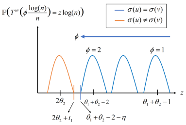
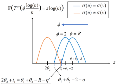
Lemma 4.1 shows that indeed the triangle count is an informative metric to distinguish the cases of $\sigma(u)=\sigma(v)$ and $\sigma(u)\neq\sigma(v)$. It is also strongly related to the distance of node features $d_{uv}$. See Figure 2a for the visualization.

4.1 Analysis of Algorithm 3.1

We begin by stating the theoretical guarantee of Algorithm 3.1 under the assumption that $\theta_{1}\geq 2\theta_{2}$, and $\theta_{1}\geq 2$.

Theorem 4.2.

Define

$$t_{1}=\inf\left\{t\geq 0:(2\theta_{2}+t)\log(\frac{2\theta_{2}+t}{2\theta_{2}})-t>1\right\},$$ (1)

Under the assumption that $\theta_{1}>2\theta_{2}\geq 2$, set in Algorithm 3.1

$$\eta=\inf\left\{t\geq 0:(\theta_{1}+\theta_{2}-2-t)\log(\frac{\theta_{1}+\theta_{2}-2-t}{\theta_{1}+\theta_{2}-2})+t>1\right\}$$

$$E_{T}=(\theta_{1}+\theta_{2}-2-\eta)\frac{\log(n)}{n}.$$ (2)

If $\theta_{1}-\theta_{2}-2-\eta>t_{1}$, then after Phase 1 in Algorithm 3.1, we already recover the communities up to a permutation with probability at least $1-o(1)$. If $t_{1}>\theta_{1}-\theta_{2}-2-\eta>0$, after Phase 2, with probability at least $1-o(1)$, Algorithm 3.1 will recover the communities up to a permutation with query complexity at most

$$O(n^{1-\epsilon}\log(n)^{3}+\log(n)),$$ (3)

where

$$\epsilon=(\theta_{1}+\theta_{2}-2-\eta)\log(\frac{\theta_{1}+\theta_{2}-2-\eta}{2\theta_{2}})-(\theta_{1}-\theta_{2}-2-\eta).$$

Theorem 4.3.

Under the assumption that $2\theta_{2}\leq 2$, $\theta_{1}\geq 2$, setting

$$\eta=\inf\left\{t\geq 0:(2\theta_{1}-2-t)\log(\frac{2\theta_{1}-2-t}{2\theta_{1}-2})+t>2\right\}$$

$$E_{T}=\frac{1}{2}(2\theta_{1}-2-\eta)\frac{\log(n)}{n},$$ (4)

the same theoretical guarantees for Algorithm  3.1, stated in Theorem 4.2, can be derived by redefining $\epsilon$ in (3) as:

$$\epsilon=(\frac{1}{2}(2\theta_{1}-2-\eta))\log(\frac{\frac{1}{2}(2\theta_{1}-2-\eta)}{2\theta_{2}})-(\frac{1}{2}(2\theta_{1}-2-\eta)-2\theta_{2}).$$

Remark 4.1.

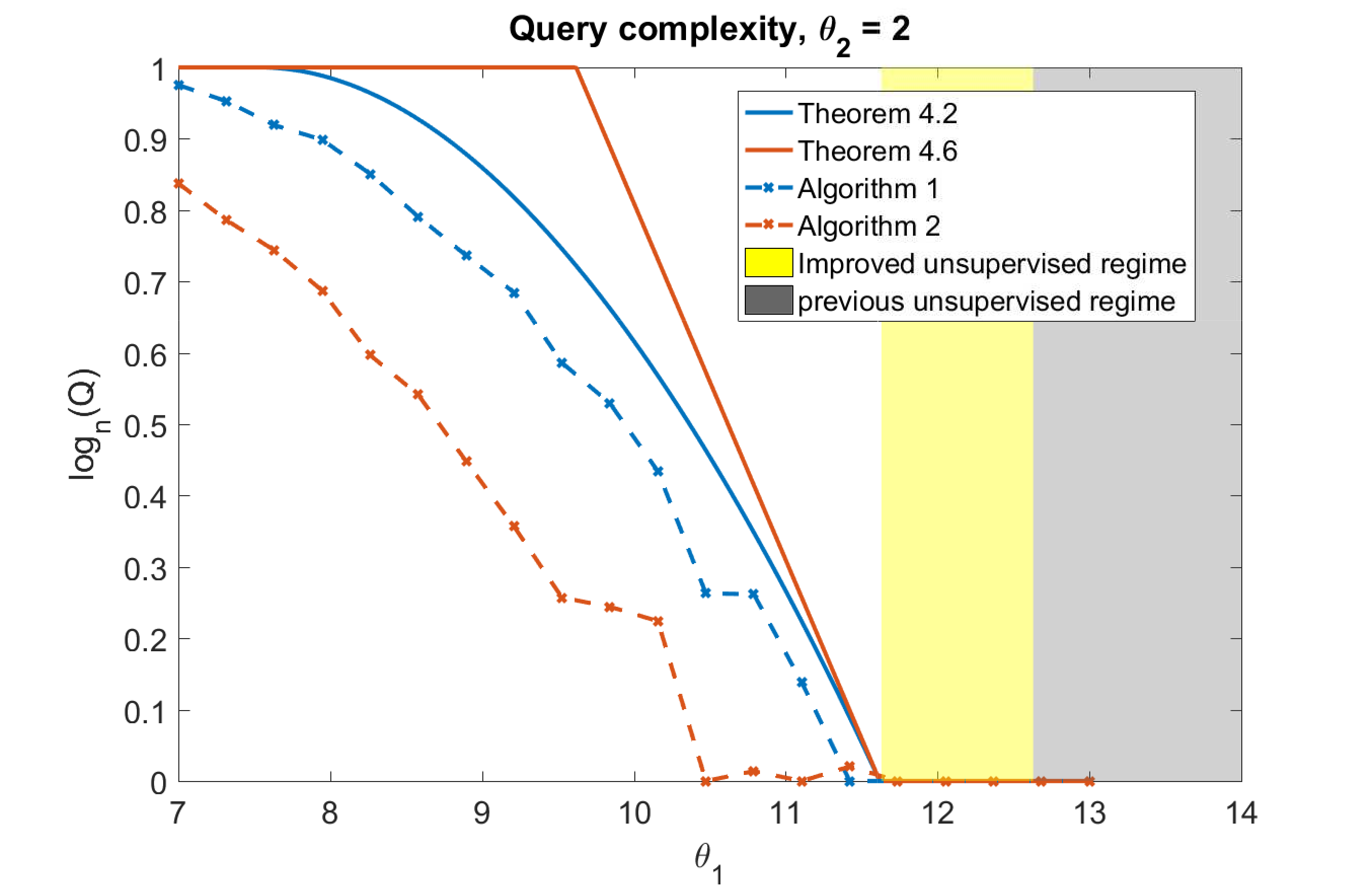
Note that for any fixed $\theta_{2}$ such that $\theta_{1}\geq 2\theta_{2}$ with $\theta_{1}\geq 2$, $1-\epsilon$ decays as $\theta_{1}$ grows. Thus, Algorithm 3.1 provides a smooth trade-off between clustering hardness and query complexity. Interestingly, we show that when $\theta_{1}-\theta_{2}-2-\eta>t_{1}$, we can achieve exact recovery without any queries. We numerically show that this result gives an improvement over the previously known bound for unsupervised methods given in (?) for a wide range of $\theta_{2}$ (See Figure 1).

Figure 1: The minimum gap between $\theta_{1}$ and $\theta_{2}$ permitted by our Theorem 4.2 versus the state-of-the-art bound of (?) in the unsupervised setting.

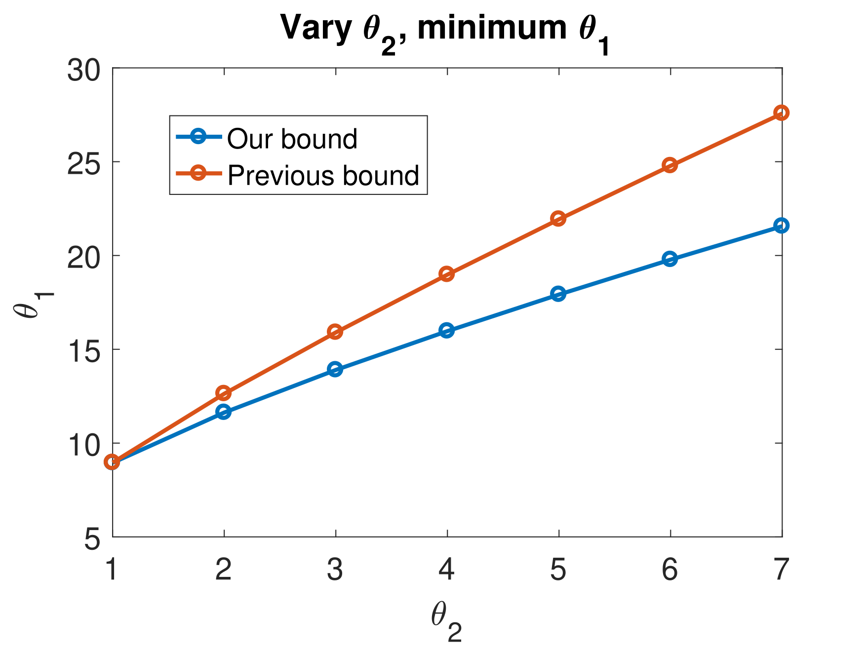
In the following, we focus on proving Theorem 4.2, since Theorem 4.3 can be proved analogously. In order to prove Theorem 4.2, we will use the theoretical guarantee of the $S^{2}$ algorithm and two technical lemmas.

Theorem 4.4 (Simplified Theorem 3 in (?)).

Let $C$ be the set of cross-cluster edges in graph $G$ with latent labels $\mathbf{\sigma}$. Let $\partial C$ be the set of nodes associated with at least $1$ cross-cluster edge. Suppose that each cluster is connected and has diameter at most $D$. If the $S^{2}$ algorithm uses at least

$$\frac{\log(2/\delta)}{\log(2)}+\lceil\log_{2}(n)\rceil+(\min(|\partial C|,|C|)-1)(\lceil\log_{2}(2D+1)\rceil+1)$$

queries, then with probability at least $1-\delta$ the $S^{2}$, the algorithm will recover the clusters exactly.

Remark 4.2.

We note that while the original analysis in (?) only uses the term $|\partial C|$ in the query complexity, the authors of (?) slightly improve it by including the term $\min(|\partial C|,|C|)$, which better serves our analysis.

Lemma 4.5.

Assume $\theta_{2}\geq 1$. Let

$$\eta=\inf\left\{t\geq 0:(\theta_{1}+\theta_{2}-2-t)\log(\frac{\theta_{1}+\theta_{2}-2-t}{\theta_{1}+\theta_{2}-2})+t>1\right\}.$$

Then, by choosing $E_{T}=(\theta_{1}+\theta_{2}-2-\eta)\frac{\log(n)}{n}$, Phase 1 of Algorithm 3.1 is guaranteed to generate a graph $G_{r}$ whose underlying communities are connected.

Lemma 4.6.

Assume $\theta_{2}\geq 1$ and set $E_{T}$ as in Lemma 4.5. Let $C$ be the set of cross-cluster edges in $G_{r}$. If $\theta_{1}-\theta_{2}-2-\eta>t_{1},$, then with probability at least $1-o(1)$, we have $|C|=0$. If $t_{1}>\theta_{1}-\theta_{2}-2-\eta>0,$, we have

$$|C|\leq\frac{\theta_{2}}{2}n^{1-\epsilon}(\log(n))^{2}$$

with probability at least $1-o(1)$, where

$$\epsilon=(\theta_{1}+\theta_{2}-2-\eta)\log(\frac{\theta_{1}+\theta_{2}-2-\eta}{2\theta_{2}})-(\theta_{1}-\theta_{2}-2-\eta)$$

Remark 4.3.

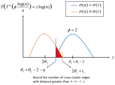
Note that while Lemma 4.5 characterizes the threshold in Phase 1 of Algorithm 3.1 that guarantees removing the most cross-cluster edges while maintaining intra-cluster connectivity, Lemma 4.6 provides a bound on the number of remaining cross-cluster edges. Such bound, together with the result stated in Theorem 4.4, is one of the key ingredients in the evaluation of the query complexity bound of Algorithm 3.1. A graphical interpretation of the parameters $t_{1}$ and $\eta$, as well as of the key steps of the proof of Lemma 4.6 is provided in Figures 2a and 2b.

We are now ready to provide the proof of Theorem 4.2.

Proof.

The first half of Theorem 4.2 directly follows from Lemma 4.5 and  4.6. Hence, in the following, we focus on the case $t_{1}>\theta_{1}-\theta_{2}-2-\eta>0$. From Lemma 4.5, we know that with probability at least $1-o(1)$ of the underlying clusters of graph $G_{r}$ (the graph returned by Phase 1) are still connected among each other. Then, by Theorem 4.4, we know that with probability at least $1-\delta$, using at most

$$\frac{\log(2/\delta)}{\log(2)}+\lceil\log_{2}(n)\rceil+(\min(|\partial C|,|C|)-1)(\lceil\log_{2}(n+1)\rceil+1)$$

queries, we can recover the communities. Finally, by Lemma 4.6, we know that with probability at least $1-o(1)$, $\min(|\partial C|,|C|)\leq|C|\leq\frac{\theta_{2}}{2}n^{1-\epsilon}\log(n)^{2}$. Hence, by union bound over all error events, we know that with probability at least $1-o(1)$, we can recover the communities with at most

$$O(n^{1-\epsilon}\log(n)^{3}+\log(n))$$

queries, by simply choosing $\delta=\frac{1}{n}$. ∎

(a) Case for $\theta_{1}-\theta_{2}-2-\eta>t_{1}$

(b) Case for $\theta_{1}-\theta_{2}-2-\eta<t_{1}$. Key idea of Lemma 4.6

(c) Case for $\theta_{1}-\theta_{2}-2-\eta<t_{1}$. Key idea of Lemma 4.8

Figure 2: Figure (a) illustrates Lemma 4.1 and the intuition behind parameters $t_{1}$ and $\eta$. Figure (b) illustrates the main idea behind the proof of Lemma 4.6. We use the error probability (red area) to compute the expected number of cross-cluster edges that are kept after Phase 1 of Algorithm 3.1. Then, we use Markov inequality to give the high probability bound for the number of cross-cluster edges in $G_{r}$. Figure (c) illustrate the idea of parameter $R$, which is chosen to be the largest number such that $T^{uv}(R\frac{\log(n)}{n})\geq 2\theta_{2}+t_{1}$ for intra-cluster edges (blue) with high probability.

4.2 Analysis of Algorithm 3.2

The next theorem provides the theoretical guarantee of Algorithm 3.2 under the assumption that $\theta_{1}\geq 2\theta_{2}$, and $\theta_{2}>1$.

Theorem 4.7.

Assume $\theta_{1}\geq 2\theta_{2}$, $\theta_{2}\geq 1$, and $2\theta_{2}+t_{1}>\theta_{1}+\theta_{2}-2-\eta$. With probability at least $1-o(1)$, Algorithm 3.2 exactly recovers the underlying clusters with query complexity at most

$$\frac{3}{2}n^{1-R/2}+2,$$

where

$$R= \sup_{\min(\theta_{1}-\theta_{2}-t_{1},2)>r>0}\Bigg{\{}(2\theta_{2}+t_{1})\log(\frac{2\theta_{2}+t_{1}}{\theta_{1}+\theta_{2}-r})$$

$$+(\theta_{1}+\theta_{2}-r-(2\theta_{2}+t_{1}))>1\Bigg{\}}.$$

Note that if $2\theta_{2}+t_{1}<\theta_{1}+\theta_{2}-2-\eta$, since Algorithm 3.2 sets the threshold for the triangle count to $2\theta_{2}+t_{1}$, it is immediate to note (see Figure 2a) that all cross-cluster edges will be removed while preserving all intra-cluster edges whose distance $\phi\frac{\log(n)}{n}$ is less than $2\frac{\log(n)}{n}$. In order to proof Theorem 4.7, we need the following lemmas.

Lemma 4.8.

Assume $\theta_{1}\geq 2\theta_{2}$, $\theta_{2}\geq 1$ and $2\theta_{2}+t_{1}>\theta_{1}+\theta_{2}-2-\eta$. All intra-cluster edges with distance less than $R$ will not be removed in $G_{r}$, where

$$R= \sup_{\min(\theta_{1}-\theta_{2}-t_{1},2)>r>0}\Bigg{\{}(2\theta_{2}+t_{1})\log(\frac{2\theta_{2}+t_{1}}{\theta_{1}+\theta_{2}-r})$$

$$+(\theta_{1}+\theta_{2}-r-(2\theta_{2}+t_{1}))>1\Bigg{\}}$$

Figure 2c provides a graphical illustration of $R$. The key idea is to find the largest $R$ such that all intra-cluster edges with distance smaller than $R$ will not be removed with high probability during Phase 1 of Algorithm 3.2.

Next, we characterize the number of disjoint components created in each cluster by Phase 1 of Algorithm 3.2. To this end (see Remark 2.1), we resort to the following lemma.

Lemma 4.9 (Modification of Theorem 8.1 in (?)).

Given a random geometric graph $RGG(n,\tau)$ with $2\tau<1$, let $\mathcal{C}_{n,\tau}$ be the probability mass function of the number of disjoint components $-1$ of $RGG(n,\tau)$, and let $\Pi_{\lambda}$ denote a Poisson distribution with parameter $\lambda$. Let $d_{TV}(\mu,\nu)\triangleq\frac{1}{2}\sum_{x=0}^{\infty}|\mu(x)-\nu(x)|$ be the total variation of the two probability mass functions $\mu$ and $\nu$ on $\mathbb{N}$. We then have

$$d_{TV}(\mathcal{C}_{n,\tau},\Pi_{\lambda_{n}(\tau)})\leq B_{n}(\tau),$$

where

$$\lambda_{n}(\tau)=n(1-\tau)^{n},\;B_{n}(\tau)=n(1-\tau)^{n}-(n-1)(1-\frac{\tau}{1-\tau})^{n}$$

The key idea of the proof of Theorem 8.1 in (?) is observing that the number of disjoint components can be related to the indicator functions of the spacing of uniform random variables. Note that these indicator functions are nothing but properly correlated Bernoulli random variables which can be approximated by a Poisson random variable where the total variation can be bounded via Stein-Chen’s method (?). See more details in (?), and the modification for our setting in the supplementary material.

Lemma 4.10 (Poisson tail bound (?)).

Let $X\sim\Pi_{\lambda}$ be a Poisson random variable with parameter $\lambda$. For all $y>0$,

$$\mathbb{P}\left(X\geq\lambda+y\right)\leq\exp\left(-\frac{y^{2}}{2(\lambda+y)}\right).$$

We are now ready to state the sketch of the proof of Theorem 4.7. First, we use Lemma 4.8 to find the largest distance $R$ such that, with high probability, all intra-cluster edges with distance smaller than $R$ will not be removed during Phase 1 of Algorithm 3.2. Next, we note that the number of disjoint components in $G_{r}$ can be upper bounded by twice the number of disjoint components in an RGG$(\frac{n}{2},R\frac{\log(n)}{n})$. Using Lemma 4.9, we approximate the number of disjoint components in RGG$(\frac{n}{2},R\frac{\log(n)}{n})$ as a Poisson random variable with parameter given in Lemma 4.9. Combining Lemma 4.9 and 4.10, we are able to establish an upper bound on the number of disjoint components in $G_{r}$, which directly leads to the query complexity bound. The rigorous proof of Theorem 4.7 is deferred to the supplementary material.

5 Experimental Results

5.1 Synthetic Datasets

(a)

(b)

Figure 3: Query Complexity of our active learning algorithms in the GBM, where we use $Q$ to denote the query complexity. Results are averaged over $20$ independent trials. The light yellow shaded area indicates the improvement of our approach compared with  (?)(grey shaded area) in the unsupervised setting. For Theorem 4.2 and 4.7, we only plot the main term in the theoretical bounds, $n^{1-\epsilon}$ and $n^{1-R/2}$.

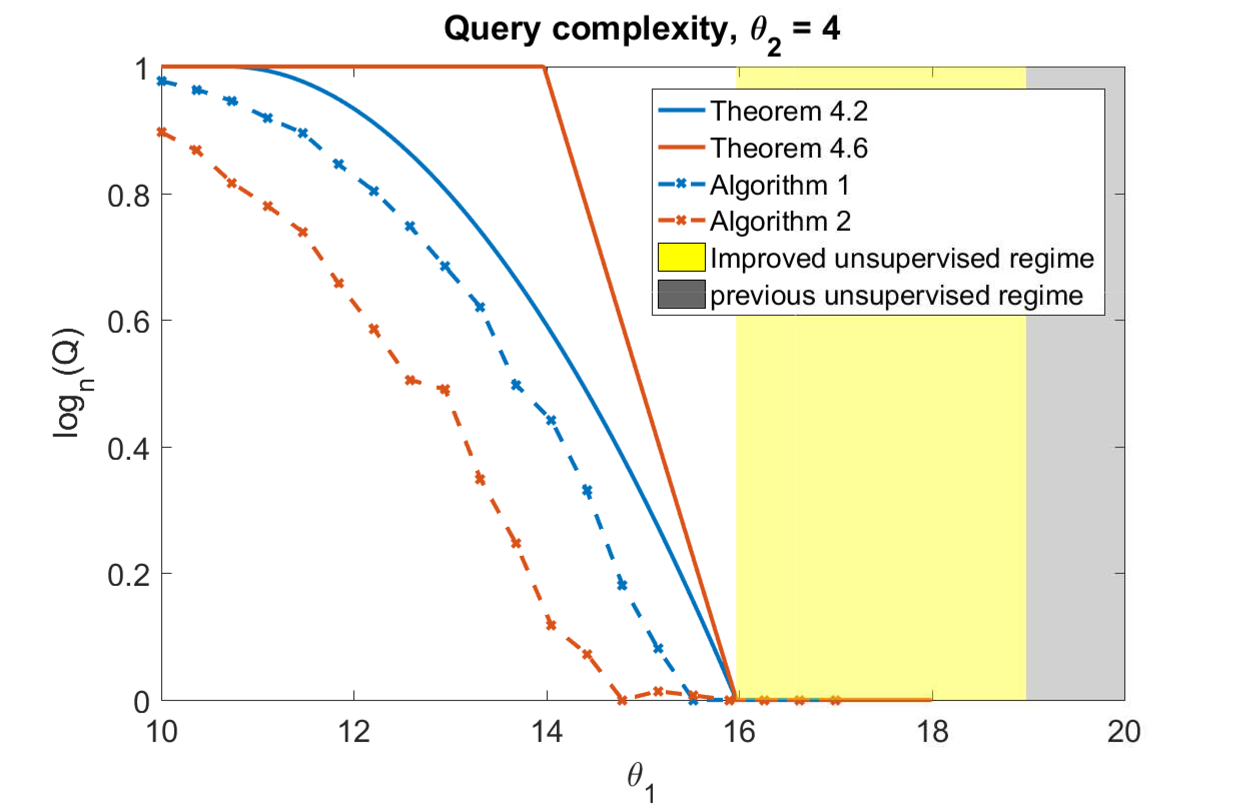
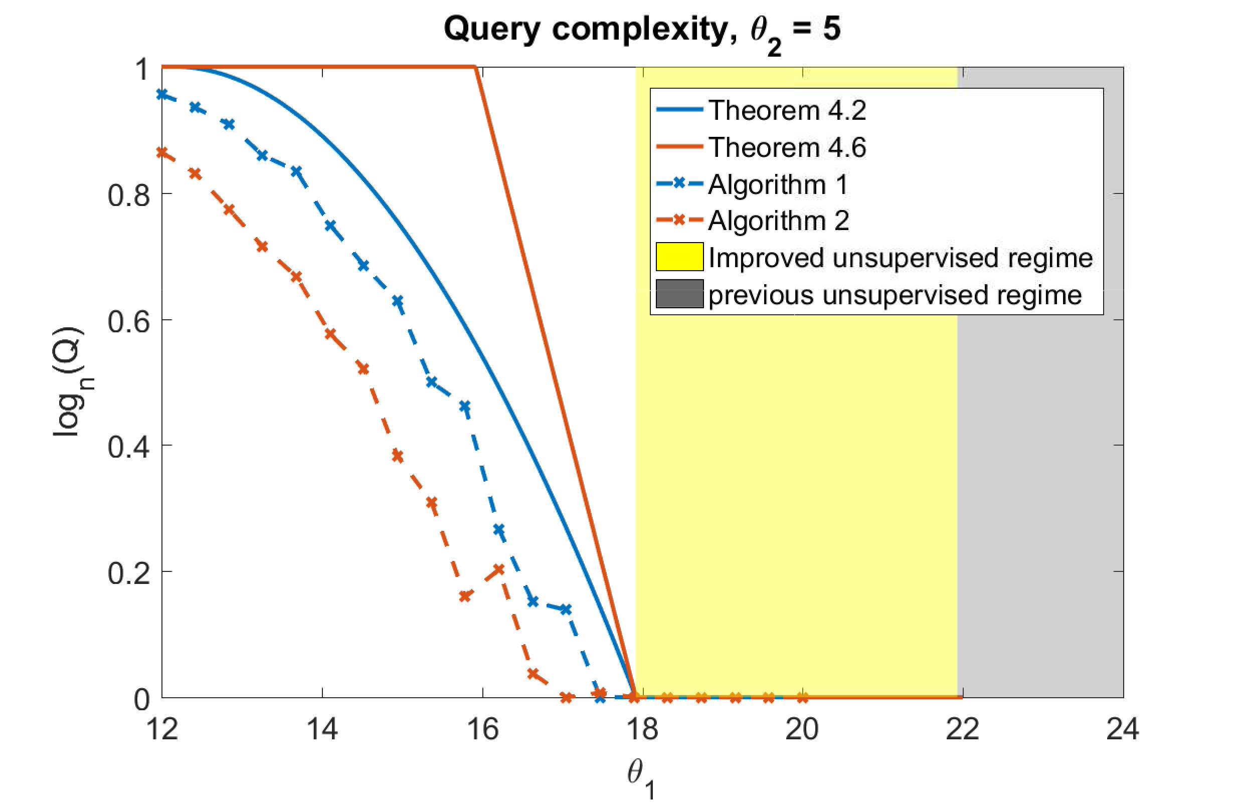
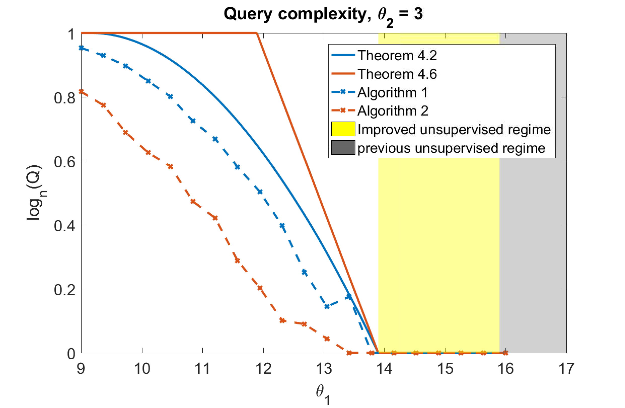
We generate random graphs using a GBM$(n,\sigma,\theta_{1},\theta_{2})$ where $n=1000$ and $\sigma$ is chosen arbitrarily among the equal-size community assignment. We plot the query complexity as a function of $\theta_{1}$ for some fixed $\theta_{2}$ in Figure 3. The figures for the other choices of $\theta_{2}$ are deferred to the supplementary material. Figure 3 plots the logarithm of the query complexity (i.e $\log_{n}(Q)$) as a function of $\theta_{1}$ for a given $\theta_{2}$. Figure 3 shows that our results improve the previously known bound for unsupervised methods given in (?) for a wide range of $\theta_{2}$, as already stated in Section 4, and our theorems capture the behavior of the query complexity for both Algorithm 3.1 and  3.2.

As expected, from Figure 3, we observe that for a fixed $\theta_{2}$, as $\theta_{1}$ decreases, we need more queries in order to achieve exact recovery. This number of queries is a very little fraction of the total number nodes, especially as $n$ grows large. For example, in our experiment we set $n=1000$. Then, using $n^{0.5}$ queries means we only use around $32$ queries, which is just $3\%$ of the total number of nodes.

Interestingly, Theorem 4.2 offers a lower query complexity bound compared with Theorem 4.7. However, from Figure 3, we can see that Algorithm 3.2 has a lower query complexity in practice, which implies that our Theorem 4.7 can be improved. In fact, in our analysis of the number of disjoint components, we only take into account the edges that with high probability will not be removed. However, there are still some edges which will be removed only with constant probability, and each of them could potentially reduce the number of disjoint components by $1$. Nevertheless, this analysis is much more complicated since these edges are not independent, and hence is left for future work.

5.2 Real Datasets

We use the following real datasets:

• Political Blogs (PB): (?) It contains a list of political blogs from the 2004 US Election classified as liberal or conservative, and links between blogs. The clusters are of roughly the same size $(586,636)$ with a total of $1222$ nodes and $16714$ edges.

• LiveJournal (LJ): (?) The LiveJournal dataset is a free online blogging social network of around $4$ million users. We extract the top two clusters of sizes (1430, 936) which consist of around $11.5$K edges.

Experimental Setting: For real-world networks $G=(V,E)$, it is hard to obtain an exact threshold as the actual values of $\theta_{1}$ and $\theta_{2}$ are unknown. Hence, following the idea proposed in (?), we use a similar but much more intuitive approach compared with (?), which consists of 3 phases. In the first phase, we set a threshold $T_{1}$. We remove all edges $(u,v)$ covered by less than $T_{1}$ triangles, and we identify $\mathcal{V}_{0}$ as the largest connected component of the obtained graph. In the second phase, we directly apply the $S^{2}$ algorithm on $\mathcal{V}_{0}$ and terminate it when we find $2$ non-singleton disjoint components in $\mathcal{V}_{0}$. Finally, in the third phase, we take majority voting to decide the cluster of $w\in V\setminus\mathcal{V}_{0}$ based on all $u\in\mathcal{V}_{0}$ such that the edge $(u,w)$ exists. Note that, in contrast with the unsupervised method used in (?), where two more hyperparameters $T_{2}$ and $T_{3}$ are required, our active learning method only needs one hyperparameter $T_{1}$. We use GMPS18 to denote the unsupervised method in (?) and Spectral to denote the standard spectral method. All results are averaged over $100$ independent trials.

Method	Accuracy		Query complexity ($\%$)
	PB	LJ	PB	LJ
Ours	$0.931$	$0.912$	$3.7$$\%$	$0.88$$\%$
Spectral	$0.53$	$0.64$	$0$	$0$
GMPS18	$0.788$	$0.777$	$0$	$0$
$S^{2}$	$0.97$	$0.999$	$47.2$$\%$	$9.2$$\%$

Table 3: Performance on real-world dataset.

For our method, we choose $T_{1}=30$ for the Political Blogs dataset and $T_{1}=5$ for the LiveJournal dataset. From Table 3, we can see that our active learning method only queries $3.7\%$ of nodes and significantly improves the accuracy from $0.788$ to $0.931$ in the Political Blogs dataset. Also, note that if we directly apply $S^{2}$ without using triangle counting, it will query 47.2$\%$ of nodes before termination. Apparently, this is too expensive in terms of query complexity. A similar result can also be observed on the LiveJournal dataset. Hence, combining triangle counting is necessary for obtaining a practical solution in the active learning framework when we have a limited query budget.

Supplement

6 Main theorem for unsupervised method

Theorem 6.1 (Restating Theorem 4,12 in (?)).

Assume $\theta_{1}\geq 2\theta_{2}$. Define

$$t_{1}=\inf\left\{t\geq 0:(2\theta_{2}+t)\log(\frac{2\theta_{2}+t}{2\theta_{2}})-t>1\right\}$$

$$t_{2}=\inf\left\{t\geq 0:(2\theta_{2}-t)\log(\frac{2\theta_{2}-t}{2\theta_{2}})+t>1\right\}$$

$$t_{3}=\sup\Bigg{\{}t:(4\theta_{2}+2t_{1})\log(\frac{4\theta_{2}+2t_{1}}{2\theta_{1}-t})$$

$$+2\theta_{1}-t-4\theta_{2}-2t_{1}>2\text{ and }0\leq t\leq 2\theta_{1}-4\theta_{2}-2t_{1}\Bigg{\}}$$

$$t_{4}=\inf\Bigg{\{}t:(4\theta_{2}-2t_{2})\log(\frac{4\theta_{2}-2t_{2}}{2\theta_{1}-t})$$

$$+2\theta_{1}-t-4\theta_{2}+2t_{2}>2\text{ and }$$

$$\max\{2\theta_{2},2\theta_{1}-4\theta_{2}+2t_{2}\}\leq t\leq\theta_{1}\Bigg{\}}$$ (5)

Then by choosing $E_{L}=(2\theta_{2}-t_{2})\frac{\log(n)}{n}$ and $E_{R}=(2\theta_{2}+t_{1})\frac{\log(n)}{n}$, we can recover the correct partition with probability at least $1-o(1)$ if $\theta_{1}-t_{4}+t_{3}>2$ or $\theta_{1}>\max\{1+t_{4},2\}$.

In the paper (?), their edge removing policy is different from both of our Algorithm 3.1 and Algorithm 3.2. For any edge $(u,v)$, it will be removed if the triangle count fall in the interval $[nE_{L},nE_{R}]$.

7 Proof of Lemma 4.5

Lemma.

Assume $\theta_{2}>1$. Let

$$\eta=\inf\left\{t\geq 0:(\theta_{1}+\theta_{2}-2-t)\log(\frac{\theta_{1}+\theta_{2}-2-t}{\theta_{1}+\theta_{2}-2})+t>1\right\}$$

Then by choosing $E_{T}=(\theta_{1}+\theta_{2}-2-\eta)\frac{\log(n)}{n}$, the underlying communities remains connected in graph $G_{r}$.

Remark 7.1.

Note that we need

$$\eta=\inf\Bigg{\{}t\geq 0:(\theta_{1}+\theta_{2}-2-t)\log(\frac{\theta_{1}+\theta_{2}-2-t}{\theta_{1}+\theta_{2}-2})+t$$

$$\geq 1+\frac{2\log\log(n)}{\log(n)}+\frac{1}{n}\frac{2(2\theta_{1}-2)t}{\theta_{1}+\theta_{2}-2}\Bigg{\}}.$$

However, since

$$\frac{2\log\log(n)}{\log(n)}+\frac{1}{n}\frac{2(2\theta_{1}-2)t}{\theta_{1}+\theta_{2}-2}\simeq o(1)$$

when $n$ is sufficiently large, we choose, for simplicity, $\eta$ as stated in Lemma 4.5.

Before proving Lemma 4.5, we need to introduce the following useful lemma

Lemma 7.1.

Given $\theta_{1}\geq 1$. With probability at least $1-\frac{1}{n}$, the number of both in-cluster and total edges are $O(n\log(n))$.

Proof.

This has been proved in (?). We include the proof here for completeness. Without loss of generality, let $u\in V_{1}$. For the other arbitrary node $v\in V_{1}$, the probability of $(u,v)\in E$ is $\frac{2\theta_{1}\log(n)}{n}$. Thus the number of in-cluster edges associate with $u$ is $Bin(\frac{n}{2}-1,\frac{2\theta_{1}\log(n)}{n})$. Hence by standard Chernoff bound, for any $c\geq 1$ we have

$$\mathbb{P}\left(Bin(\frac{n}{2}-1,\frac{2\theta_{1}\log(n)}{n})\geq(1+c)(\frac{n}{2}-1)(\frac{2\theta_{1}\log(n)}{n})\right)$$

$$\leq\exp\left(-\frac{c}{3}(\frac{n}{2}-1)(\frac{2\theta_{1}\log(n)}{n})\right)$$

$$=\exp\left(-\frac{c}{3}(1-o(1))\theta_{1}\log(n))\right)$$

$$=n^{-(1-o(1))\frac{c}{3}\theta_{1}}\stackrel{{\scriptstyle(a)}}{{\leq}}n^{-(1-o(1))\frac{c}{3}},$$

where (a) is due to our assumption $\theta_{1}\geq 1$. Hence if we choose $c>6$, then with probability at least $1-\frac{1}{n^{2}}$ the number of in-cluster edges associate with $u$ is $O(\log(n))$. By union bound over all nodes, we know that with probability at least $1-\frac{1}{n}$, the number of in-cluster edges is $O(n\log(n))$. For the number of total edges, we can apply the same argument or simply by the fact that $\theta_{1}\geq\theta_{2}$. ∎

Now we are ready to prove Lemma 4.5.

Proof.

From the classical connectivity result of RGG$(\frac{n}{2},\theta\frac{\log(n)}{n})$, we need $\theta>2$ in order to have $2$ connected components with high probability. Note that the critical radius of $RGG(\frac{n}{2},\theta\frac{\log(n)}{n})$ is:

$$\theta\frac{\log(n)}{n}=\frac{\log(\frac{n}{2})}{\frac{n}{2}},$$

which means $\theta=2-\frac{2\log(2)}{\log(n)}=2-o(1)$. For simplicity we will set the critical value to be $2$ which is sufficient for the connectivity.

Hence if we will not remove any edges such that $d_{uv}\leq\frac{2\log(n)}{n}$, then the underlying communities remain connected in graph $G_{r}$.

From Lemma 4.1 we know that for an in-cluster edge $(u,v)$ with distance $x=\frac{\phi\log(n)}{n}$, the number of triangles covering such edge is

$$T^{uv}(x)\sim Bin(\frac{n}{2}-2,(2\theta_{1}-\phi)\frac{\log(n)}{n})$$

$$+\mathbf{1}\{\phi\leq 2\theta_{2}\}Bin(\frac{n}{2},(2\theta_{2}-\phi)\frac{\log(n)}{n}).$$

Note that the mean of both Binomial decreases as $\phi$ increases. Hence for any threshold $t$ independent of $\phi$, we have:

$$\mathbb{P}\left(T^{uv}(\phi\frac{\log(n)}{n})\geq t\right)\geq\mathbb{P}\left(T^{uv}(2\frac{\log(n)}{n})\geq t\right).$$

for all $\phi\leq 2$ when $\sigma(u)=\sigma(v)$. Now by assumption we have $2\theta_{2}\geq 2$. Then from Lemma 4.1 we know that

$$T^{uv}(\frac{2\log(n)}{n})\sim Bin(\frac{n}{2}-2,(2\theta_{1}-2)\frac{\log(n)}{n})$$

$$+Bin(\frac{n}{2},(2\theta_{2}-2)\frac{\log(n)}{n}).$$

Hence it is sufficient to derive the threshold based on the distribution of $T^{uv}(\frac{2\log(n)}{n})$. Next, from Lemma 7.1 we know that with probability at least $1-\frac{1}{n}$, the number of total edges will be $O(n\log(n))$. Denoting $p=(2\theta_{1}-2)\frac{\log(n)}{n}$, and $q=(2\theta_{2}-2)\frac{\log(n)}{n}$, by Chernoff bound we have:

$$\mathbb{P}\left(T^{uv}(\frac{2\log(n)}{n})\leq nE_{T}\right)$$

$$\leq\inf_{\xi>0}\exp(\xi nE_{T})(1-p+pe^{-\xi})^{\frac{n}{2}-2}(1-q+qe^{-\xi})^{\frac{n}{2}}$$

$$=\inf_{\xi>0}\exp(\xi nE_{T}+(\frac{n}{2}-2)\log(1+p(e^{-\xi}-1))+\frac{n}{2}(1+q(e^{-\xi}-1)))$$

$$\stackrel{{\scriptstyle(a)}}{{\leq}}\inf_{\xi>0}\exp(\xi nE_{T}+(\frac{n}{2}-2)\log(\exp(p(e^{-\xi}-1)))$$

$$+\frac{n}{2}\log(\exp(q(e^{-\xi}-1))))$$

$$=\inf_{\xi>0}\exp(\xi nE_{T}+(\frac{n}{2}-2)(p(e^{-\xi}-1))+\frac{n}{2}(q(e^{-\xi}-1)))$$

$$\stackrel{{\scriptstyle(b)}}{{\leq}}\exp\Bigg{(}-\Bigg{[}(\theta_{1}+\theta_{2}-2-\eta)\log(\frac{\theta_{1}+\theta_{2}-2-\eta}{\theta_{1}+\theta_{2}-2})$$

$$+\eta-\frac{1}{n}\frac{2\eta(2\theta_{1}-2)}{\theta_{1}+\theta_{2}-2}\Bigg{]}\log(n)\Bigg{)}$$

$$\stackrel{{\scriptstyle(c)}}{{\leq}}\frac{1}{n(\log(n))^{2}}$$

where for (a) we use $1+x\leq e^{x},\forall x\in\mathbb{R}$. For (b) we simply choose $\xi=-\log(\frac{\theta_{1}+\theta_{2}-2-\eta}{\theta_{1}+\theta_{2}-2})$. Inequality (c) follows by our choice of $\eta$. See Remark 7.1 for the detail discussion. Then, by union bound over all edges, we know that, the probability that exists at least one edge $(u,v)$ with $\sigma(u)=\sigma(v)$ and distance $x\leq\frac{2\log(n)}{n}$ such that its associated triangle count satisfies $T^{uv}(x)\leq nE_{T}$, is smaller or equal than $O(\frac{n\log(n)}{n(\log(n))^{2}})$. From this, it follows immediately that all the edges $(u,v)$ with $\sigma(u)=\sigma(v)$ have $T^{uv}(x)\geq nE_{T}$ with probability $1-O(\frac{n\log(n)}{n(\log(n))^{2}})=1-o(1)$, if $x\leq\frac{2\log(n)}{n}$. Combining this with the fact that the random geometric graph with $\frac{n}{2}$ nodes will be connected with high probability if the threshold is greater than $\frac{2\log(n)}{n}$, we complete the proof. ∎

8 Proof of Lemma 4.6

Lemma.

Assume $\theta_{2}>1$ and set $E_{T}$ as in Lemma 4.5. Let $C$ be the set of cross-cluster edges in $G_{r}$. If

$$\theta_{1}-\theta_{2}-2-\eta>t_{1},$$

then with probability at least $1-o(1)$ we have $|C|=0$. If

$$t_{1}>\theta_{1}-\theta_{2}-2-\eta>0,$$

then we have

$$|C|\leq\frac{\theta_{2}}{2}n^{1-\epsilon}(\log(n))^{2}$$

with probability at least $1-o(1)$, where

$$\epsilon=(\theta_{1}+\theta_{2}-2-\eta)\log(\frac{\theta_{1}+\theta_{2}-2-\eta}{2\theta_{2}})-(\theta_{1}-\theta_{2}-2-\eta)$$

To prove the first half of this lemma, we need the next lemma from (?) which provides a bound on the triangle count of any edge $(u,v)$ such that $\sigma(u)\neq\sigma(v)$. Note that when $\sigma(u)\neq\sigma(v)$ the distribution of the triangle count for $(u,v)$ is independent of $d_{uv}$ (see Lemma 4.1). Hence, to simplify the notation, we just use $T^{uv}$ to denote the triangle count when we condition on $\sigma(u)\neq\sigma(v)$.

Lemma 8.1 (Simplified Lemma 13 in (?)).

Suppose the graph is generated from GBM$(n,\sigma,\frac{\theta_{1}\log(n)}{n},\frac{\theta_{2}\log(n)}{n})$. For each edge $(u,v)$ such that $\sigma(u)\neq\sigma(v)$, the associated triangle count $T^{uv}$ is less than $(2\theta_{2}+t_{1})\log(n)$ with probability at least $1-\frac{1}{n\log(n)^{2}}$.

Now we are ready to prove Lemma 4.6

Proof.

The proof of the case $\theta_{1}-\theta_{2}-2-\eta>t_{1}$ follows directly from Lemma 4.5, Lemma 8.1, Lemma 7.1 and Lemma 4.1. Recall that for any edge $(u,v)$ such that $\sigma(u)\neq\sigma(v)$, $T^{uv}$ is a Binomial random variable with mean $2(1-\frac{2}{n})\theta_{2}\log(n)$. Note that $\theta_{1}-\theta_{2}-2-\eta>t_{1}$ is equivalent to $\theta_{1}+\theta_{2}-2-\eta>2\theta_{2}+t_{1}$. By Lemma 8.1 we know that $T^{uv}$ is less than $(2\theta_{2}+t_{1})\log(n)$ with probability at least $1-\frac{1}{n\log(n)^{2}}$. This implies that $T^{uv}$ is larger than $nE_{T}=(\theta_{1}+\theta_{2}-2-\eta)\log(n)$ with probability at most $\frac{1}{n\log(n)^{2}}$. Then by Lemma 7.1 we know that the number of cross-edges is at most $O(n\log(n))$ with probability at least $1-\frac{1}{n}$. Applying the union bound over all cross-edges, we show that setting the threshold to $nE_{T}$ with $E_{T}$ as in Lemma 4.5, we will remove all cross-cluster edges if $\theta_{1}-\theta_{2}-2-\eta>t_{1}$.

Now we prove the result for the case $t_{1}>\theta_{1}-\theta_{2}-2-\eta>0$. First we compute the first moment of $|C|$. Let $\mathbf{A}^{(r)}$ be the adjacency matrix of $G_{r}$. By the edge removing policy in our algorithm, we have

$$\mathbb{E}\left[|C|\right]=\mathbb{E}\left[\sum_{u<v,\sigma(u)\neq\sigma(v)}A_{uv}^{(r)}\right]=(\frac{n}{2})^{2}\mathbb{P}\left(A_{uv}^{(r)}=1\right)$$

where the last equality is due to symmetry of the cross-edges. Then by Bayes’ rule we have

$$\mathbb{P}\left(A_{uv}^{(r)}=1\right) =\mathbb{P}\left(A_{uv}^{(r)}=1\big{|}A_{uv}=1\right)\mathbb{P}\left(A_{uv}=1\right)$$

$$+\mathbb{P}\left(A_{uv}^{(r)}=1\big{|}A_{uv}=0\right)\mathbb{P}\left(A_{uv}=0\right)$$

$$=\mathbb{P}\left(A_{uv}^{(r)}=1\big{|}A_{uv}=1\right)\mathbb{P}\left(A_{uv}=1\right),$$

where the last equality follows the fact that with probability $1$, $A_{uv}=0$ implies $A_{uv}^{(r)}=0$ since we do not add edges. It is easy to see that

$$\mathbb{P}\left(A_{uv}=1\right)=\frac{2\theta_{2}\log(n)}{n}$$

from the generative model. For the other probability, based on Lemma 4.1 and our edge removing policy we have

$$\mathbb{P}\left(A_{uv}^{(r)}=1\big{|}A_{uv}=1\right)=\mathbb{P}\left(T^{uv}\leq nE_{T}\right)$$

Hence so far we have

$$\mathbb{E}|C|=\frac{\theta_{2}n\log(n)}{2}\mathbb{P}\left(T^{uv}\leq nE_{T}\right)$$ (6)

In order to get the more explicit result, we can further upper bound $\mathbb{P}\left(T^{uv}\leq nE_{T}\right)$ by Chernoff bound as following. For simplicity we denote $q^{\prime}=\frac{2\theta_{2}\log(n)}{n}$.

$$\mathbb{P}\left(T^{uv}\leq nE_{T}\right)\leq\inf_{\xi>0}\exp(\xi nE_{T})(1+q^{\prime}(e^{-\xi}-1))^{n-2}$$

$$=\inf_{\xi>0}\exp(\xi nE_{T}+(n-2)\log(1+q^{\prime}(e^{-\xi}-1)))$$

$$\leq\inf_{\xi>0}\exp(\xi nE_{T}+(n-2)\log(\exp(q^{\prime}(e^{-\xi}-1))))$$

$$=\inf_{\xi>0}\exp(\xi nE_{T}+(n-2)q^{\prime}(e^{-\xi}-1))$$

$$\leq\exp\Bigg{(}-\Bigg{[}(\theta_{1}+\theta_{2}-2-\eta)\log(\frac{\theta_{1}+\theta_{2}-2-\eta}{2\theta_{2}})$$

$$-(\theta_{1}-\theta_{2}-2-\eta)+\frac{2(\theta_{1}-\theta_{2}-2-\eta)}{n}\Bigg{]}\log(n)\Bigg{)}$$

$$\stackrel{{\scriptstyle(a)}}{{\leq}}n^{-\epsilon}$$ (7)

Note that inequality (a) is due to our choice of $\epsilon$ and the assumption $(\theta_{1}-\theta_{2}-2-\eta)>0$. Using (8) we can upper bound (6) as following:

$$\mathbb{E}\left[|C|\right]\leq\frac{\theta_{2}}{2}n^{1-\epsilon}\log(n)$$ (8)

Then, applying Markov inequality:

$$\mathbb{P}\left(|C|\geq\mathbb{E}\left[|C|\right]\log(n)\right)\leq\frac{1}{\log(n)}=o(1)$$ (9)

and combining (9) with (8), we can show that with probability at least $1-o(1)$, $|C|\leq\frac{\theta_{2}}{2}n^{1-\epsilon}(\log(n))^{2}$ which completes the proof. ∎

9 Proof of Lemma 4.8

Lemma.

Assume $\theta_{1}\geq 2\theta_{2}$, $\theta_{2}\geq 1$, and $2\theta_{2}+t_{1}>\theta_{1}+\theta_{2}-2-\eta$. All the in-cluster edges with distance in feature space less than $R$ will not be removed in $G_{r}$, where

$$R= \sup_{\min(\theta_{1}-\theta_{2}-t_{1},2)>r>0}\Bigg{\{}(2\theta_{2}+t_{1})\log(\frac{2\theta_{2}+t_{1}}{\theta_{1}+\theta_{2}-r})$$ (10)

$$+(\theta_{1}+\theta_{2}-r-(2\theta_{2}+t_{1}))>1\Bigg{\}}$$ (11)

Proof.

From Lemma 4.1 we know that for an in-cluster edge $(u,v)$ with distance $x=\frac{\phi\log(n)}{n}$, the number of triangles covering such edge is

$$T^{uv}(x)\sim Bin(\frac{n}{2}-2,(2\theta_{1}-\phi)\frac{\log(n)}{n})$$

$$+\mathbf{1}\{\phi\leq 2\theta_{2}\}Bin(\frac{n}{2},(2\theta_{2}-\phi)\frac{\log(n)}{n}).$$

Also, the probability that such edge being removed is monotonically increasing in $x$ from the similar argument in the proof of Lemma 4.5. Then from assumption we know that we can only guarantee to keep all edges with distance $R<2\leq 2\theta_{2}$ with high probability for some $R$. In order to choose the best possible $R$, similarly to Lemma 4.5, we leverage again the tail bound of Poisson Binomial distribution. More specifically, let us denote $p=(2\theta_{1}-\phi)\frac{\log(n)}{n}$ and $q=(2\theta_{2}-\phi)\frac{\log(n)}{n}$. The probability that an in-cluster edge $(u,v)$ with $d_{uv}=x=\phi\frac{\log(n)}{n}$ will be removed is

$$\mathbb{P}\left(T^{uv}(x)\leq(2\theta_{2}+t_{1})\log(n)\right)$$

$$\leq\inf_{\xi>0}\exp(\xi(2\theta_{2}+t_{1})\log(n)+(\frac{n}{2}-2)\log(1-p+pe^{-\xi})$$

$$+\frac{n}{2}\log(1-q+qe^{-\xi}))$$

$$\leq\inf_{\xi>0}\exp(\xi(2\theta_{2}+t_{1})\log(n)+(\frac{n}{2}-2)p(e^{-\xi}-1)+\frac{n}{2}q(e^{-\xi}-1))$$

$$\stackrel{{\scriptstyle(a)}}{{\leq}}\exp\bigg{(}-[(2\theta_{2}+t_{1})\log(\frac{(2\theta_{2}+t_{1})}{\theta_{1}+\theta_{2}-\phi})+(2\theta_{2}+t_{1})$$

$$-(\theta_{1}+\theta_{2}-\phi)]\log(n)$$

$$+\frac{4\theta_{1}-2\phi}{\theta_{1}+\theta_{2}-\phi}[(\theta_{1}+\theta_{2}-\phi)-(2\theta_{2}+t_{1})]\frac{\log(n)}{n}\bigg{)}$$

$$\stackrel{{\scriptstyle(b)}}{{\leq}}\frac{1}{n\log(n)^{2}}$$

Note that for inequality (a), we choose $\xi=-\log(\frac{2\theta_{2}+t_{1}}{\theta_{1}+\theta_{2}-\phi})$. This is a valid choice for all $0<\phi<\theta_{1}-\theta_{2}-t_{1}$. Let $M=\min(\theta_{1}-\theta_{2}-t_{1},2)$. Now we want to choose the best possible $\phi=R$ for the inequality (b) to hold:

$$R=\sup_{M>\phi>0}\Bigg{\{}(2\theta_{2}+t_{1})\log(\frac{(2\theta_{2}+t_{1})}{\theta_{1}+\theta_{2}-\phi})+(2\theta_{2}+t_{1})-(\theta_{1}+\theta_{2}-\phi)$$

$$-\frac{1}{n}\frac{4\theta_{1}-2\phi}{\theta_{1}+\theta_{2}-\phi}[(\theta_{1}+\theta_{2}-\phi)-(2\theta_{2}+t_{1})]-\frac{2\log(\log(n))}{\log(n)}\geq 1\Bigg{\}}.$$

Note that the last two terms in the above expression are $o(1)$. Hence, for $n$ large enough we can ignore them, from which (10) follows immediately. Next, note that our assumption $2\theta_{2}+t_{1}>\theta_{1}+\theta_{2}-2-\eta$ already implies that $R$ given in (10) is such that $R<2$. See Figure 2c for the illustration. Hence, by using Lemma 7.1, which states that that the number of in-cluster edges is $O(n\log(n))$ with probability at least $1-\frac{1}{n}$, by recalling from Section 7 that the probability of removing an edge with distance smaller than $R<2$ is at most $\frac{1}{n(\log(n))^{2}}$, and by applying union bound over all in-cluster edges, it follows immediately that with probability at least $1-o(1)$ all in-cluster edges with distance less then $R$ will not be removed. This completes the proof. ∎

10 Proof of Lemma 4.9

Lemma (Modification of Theorem 8.1 in (?)).

Given a random geometric graph, $RGG(n,\tau)$, with $2\tau<1$, let $\mathcal{C}_{n,\tau}$ be the probability mass function of the number of disjoint components $-1$ of $RGG(n,\tau)$ and let $\Pi_{\lambda}$ denote a Poisson distribution with parameter $\lambda$. Let $d_{TV}(\mu,\nu)\triangleq\frac{1}{2}\sum_{x=0}^{\infty}|\mu(x)-\nu(x)|$ be the total variation of the two probability mass functions $\mu$ and $\nu$ on $\mathbb{N}$. Then we have

$$d_{TV}(\mathcal{C}_{n,\tau},\Pi_{\lambda_{n}(\tau)})\leq B_{n}(\tau),$$

where

$$\lambda_{n}(\tau)=n(1-\tau)^{n},\;B_{n}(\tau)=n(1-\tau)^{n}-(n-1)(1-\frac{\tau}{1-\tau})^{n}$$

Remark 10.1.

This is a slight modification of Theorem 8.1 in (?). In fact, in (?) the authors assume that the nodes are distributed on an unit length interval rather than on a unit length circle as in our setting. In the following we show how the modification can be done for our case. Note that although we are aware that the authors of (?) pointed out that the result for the unit length circle had been already established in (?), we have no access to that paper and hence we prove it here again for completeness.

Proof.

Let us first assume that we are in the same setting as (?), where the nodes are uniformly distributed on the unit length interval. Let $X_{1},...,X_{n}$ denote the ordered node positions, i.e. $0\leq X_{1}\leq X_{2}\leq...\leq X_{n}\leq 1$. Further, let $L_{i}$ be the spacing, i.e. $L_{i}=X_{i}-X_{i-1},\;\forall i=1,...,n+1$ where we let $X_{0}=0$ and $X_{n+1}=1$. It is clear that $\sum_{i=1}^{n+1}L_{i}=1$. Next, let $\chi_{i}(\tau)=\mathbf{1}\{L_{i}>\tau\},\forall i=2,...,n$. It is clear that $\sum_{i=2}^{n}\chi_{i}(\tau)+1$ is exactly the number of disjoint components and thus $\sum_{i=2}^{n}\chi_{i}(\tau)$ has probability mass function $\mathcal{C}_{n,\tau}$. Theorem 8.1 in (?) shows that

$$d_{TV}(\mathcal{C}_{n,\tau},\Pi_{\lambda_{n}^{\prime}(\tau)})\leq B_{n}^{\prime}(\tau),$$

$$\lambda_{n}^{\prime}(\tau)=(n-1)(1-\tau)^{n},$$

$$B_{n}^{\prime}(\tau)=(n-1)(1-\tau)^{n}-(n-2)(1-\frac{\tau}{1-\tau})^{n}$$

Now we turn back to our setting, where the nodes are uniformly distributed on the unit length circle. We observe that by unraveling our circle at an arbitrary place, we obtain the unit length interval and the nodes can be still ordered as $X_{1},...,X_{n}$. Similarly we can define the spacing to be $L_{i}=X_{i}-X_{i-1},\;\forall i=1,...,n+1$. However, beside defining $\chi_{i}(\tau)=\mathbf{1}\{L_{i}>\tau\},\forall i=2,...,n$, we also define $\chi_{1}=\mathbf{1}\{L_{1}+L_{n+1}>\tau\}$. Note that $L_{1}+L_{n+1}$ is exactly the distance of $X_{1}$ to $X_{n}$ in the circle. Also note that by symmetry, $\chi_{1}$ is identically distributed as $\chi_{2}(\tau),...,\chi_{n}(\tau)$. Thus the number of disjoint components in our case would be $\sum_{i=1}^{n}\chi_{i}(\tau)+1$ and hence we sum one more indicator random variable $\chi_{1}(\tau)$ compare to the case in (?). Hence, following the same proof of Theorem 8.1 in (?) we have Lemma 4.9. ∎

11 Proof of Theorem 4.7

Theorem.

Assume $\theta_{1}\geq 2\theta_{2}$, $\theta_{2}\geq 1$, and $2\theta_{2}+t_{1}>\theta_{1}+\theta_{2}-2-\eta$. With probability at least $1-o(1)$, Algorithm 3.2 exactly recovers the clusters with query complexity at most

$$\frac{3}{2}n^{1-R/2}+2,$$

where

$$R= \sup_{\min(\theta_{1}-\theta_{2}-t_{1},2)>r>0}\Bigg{\{}(2\theta_{2}+t_{1})\log(\frac{2\theta_{2}+t_{1}}{\theta_{1}+\theta_{2}-r})$$

$$+(\theta_{1}+\theta_{2}-r-(2\theta_{2}+t_{1}))>1\Bigg{\}}.$$

Proof.

From Lemma 8.1, we know that with probability at least $1-o(1)$ we remove all cross-cluster edges in Phase 1. Hence in the following, we will focus on bounding the query complexity of our Algorithm 3.2.

Let $Z$ be the number of disjoint components in $G_{r}$ and let $C_{n/2}(R\frac{\log(n)}{n})+1$ be the number of disjoint components in $RGG(\frac{n}{2},R\frac{\log(n)}{n})$, where $R$ is chosen according to Lemma 4.8. Note that $C_{n}(\tau)\sim\mathcal{C}_{n,\tau}$. It is obvious that for all $t$,

$$\mathbb{P}\left(Z<t\right)\leq\mathbb{P}\left(2(C_{n/2}(R\frac{\log(n)}{n})+1)<t\right)$$ (12)

due to our choice of $R$. Then by Lemma 4.9 we have

$$d_{TV}(\mathcal{C}_{\tilde{n},\tau},\Pi_{\lambda_{\tilde{n}}(\tau)})\leq B_{\tilde{n}}(\tau),\;\tilde{n}=\frac{n}{2},\;\tau=R\frac{\log(n)}{n}$$

Note that

$$B_{\tilde{n}}(\tau)=\tilde{n}(1-\tau)^{\tilde{n}}-(\tilde{n}-1)(1-\frac{\tau}{1-\tau})^{\tilde{n}}$$

$$=\tilde{n}\left[(1-\tau)^{\tilde{n}}-(1-\frac{\tau}{1-\tau})^{\tilde{n}}\right]+(1-\frac{\tau}{1-\tau})^{\tilde{n}}$$

$$\stackrel{{\scriptstyle(a)}}{{=}}\tilde{n}(-\tau+\frac{\tau}{1-\tau})\tau^{\tilde{n}-1}\left[1+\frac{1}{1-\tau}+(\frac{1}{1-\tau})^{2}+\cdots+(\frac{1}{1-\tau})^{\tilde{n}-1}\right]$$

$$+(1-\frac{\tau}{1-\tau})^{\tilde{n}}$$

$$=\tilde{n}\tau^{\tilde{n}+1}\left[\frac{1}{1-\tau}+(\frac{1}{1-\tau})^{2}+\cdots+(\frac{1}{1-\tau})^{\tilde{n}}\right]+(1-\frac{\tau}{1-\tau})^{\tilde{n}}$$

$$=\tilde{n}\tau^{\tilde{n}+1}\frac{1-(1-\tau)^{-\tilde{n}}}{1-\tau-1}+(1-\frac{\tau}{1-\tau})^{\tilde{n}}$$

$$=\tilde{n}\tau^{\tilde{n}}[(1-\tau)^{-\tilde{n}}-1]+(1-\frac{\tau}{1-\tau})^{\tilde{n}}$$

$$\stackrel{{\scriptstyle(b)}}{{\leq}}\tilde{n}\tau^{\tilde{n}}\exp(\tilde{n}\tau)+(1-\frac{\tau}{1-\tau})^{\tilde{n}}$$

where for the equality (a) we use the simple algebra fact $x^{n}-y^{n}=(x-y)(x^{n-1}+x^{n-2}y+...+y^{n-1})$. The inequality (b) follows from the elementary fact $1+x\leq\exp(x)\;\forall x\in\mathbb{R}$. The first term can be further simplify as

$$\tilde{n}\tau^{\tilde{n}}\exp(\tilde{n}\tau)=\exp(\frac{R\log(n)}{2}+\log(\frac{n}{2})+\frac{n}{2}\log(\frac{R\log(n)}{n}))$$

$$=\exp(\frac{R\log(n)}{2}+\log(\frac{n}{2})+\frac{n}{2}\log(R\log(n))-\frac{n}{2}\log(n))=o(1)$$

The second term can be bounded as

$$(1-\frac{\tau}{1-\tau})^{\tilde{n}}\leq\exp(-\tilde{n}\frac{\tau}{1-\tau})=\exp(-\frac{R\log(n)}{2(1-\tau)})=o(1)$$

due to the fact $1-\tau=1-o(1)$. Together we have $B_{\tilde{n}}(\tau)=o(1)$. Thus we have

$$\mathbb{P}\left(2(C_{n/2}(R\frac{\log(n)}{n})+1)<t\right)$$

$$\leq\mathbb{P}\left(2(\Pi_{\lambda_{\tilde{n}}(R\frac{\log(n)}{n})}+1)<t\right)+o(1)\;\forall t$$ (13)

Then we can apply Lemma 4.10 to bound the tail probability of Poisson. Choose $y=\frac{1}{2}\lambda$ we have

$$\mathbb{P}\left(\Pi_{\lambda}\geq\lambda+y\right)\leq\exp(-\frac{y^{2}}{2(\lambda+y)})=\exp(-\frac{\lambda}{12})$$ (14)

Moreover we have

$$\lambda_{\tilde{n}}(R\frac{\log(n)}{n})=\tilde{n}(1-\frac{R\log(n)}{n})^{\tilde{n}}$$

It is easy to upper and lower bound this value as following

$$\tilde{n}(1-\frac{R\log(n)}{n})^{\tilde{n}}\leq\frac{n}{2}\exp(-\frac{R\log(n)}{2})=\frac{n^{1-R/2}}{2}$$ (15)

$$\tilde{n}(1-\frac{R\log(n)}{n})^{\tilde{n}}\geq\frac{n}{2}\exp(-\tilde{n}\frac{\tau}{1-\tau})$$

$$=\frac{n}{2}\exp(-(1+o(1))\frac{R\log(n)}{2})=\frac{n^{(1-(1+o(1))R/2)}}{2}$$ (16)

where we use the elementary inequality $1-x\geq\exp(1-\frac{x}{1-x})\;\forall x<1$ and the fact that $1-\tau=1-o(1)$. By our choice of $R$ we know that $1-R/2>0$. Thus plugging the lower bound (16) into (14) we get $\exp(-\frac{\lambda}{12})=o(1)$ by choosing $\lambda=\lambda_{\tilde{n}}(R\frac{\log(n)}{n})$. This means that with probability at least $1-o(1)$ we have

$$\Pi_{\lambda_{\tilde{n}}(R\frac{\log(n)}{n})}\leq\frac{3}{2}\lambda_{\tilde{n}}(R\frac{\log(n)}{n})\leq\frac{3}{4}n^{1-R/2}$$

Combine this with (12) and  (11) we have shown that with probability at least $1-o(1)$, the number of disjoint components in $G_{r}$ is at most

$$\frac{3}{2}n^{1-R/2}+2,$$

and this completes the proof. ∎

12 The $S^{2}$ algorithm

Here we include the original $S^{2}$ algorithm in (?) for completeness. Here we use $f(x)$ to denote the label of node $x$.

Input : Graph $G$, query complexity budget $\mathcal{Q}(\delta)$

Output : A partition of $V$

Main Algorithm: $L\leftarrow\emptyset$

while 1 do

       $x\leftarrow$ Uniformly at random pick an unlabeled node.

       do

             Add $(x,f(x))$ to $L$

             Remove all hyperedges containing nodes with different label from $G$.

             if more than $\mathcal{Q}(\delta)$ queries are used then

                   Return the remaining connected components of $G$ or LabelCompletion$(G,L)$

             end if

            

      while $x\leftarrow MSSP(G,L)$ exists

end while

Algorithm 12.3 ($S^{2}$).

Input : Graph $G$, label list $L$

Output : The midpoint of shortest-shortest path

Main Algorithm:

for each $v,u\in L$ such that $u,v$ has different label do

       $P_{v,u}\leftarrow$ shortest path between $v,u$ in $G$.

       $l_{u,v}\leftarrow$ length of $P_{u,v}$.($=\infty$ if doesn’t exist)

      

end for

$(v^{*},u^{*})=\arg\min l_{u,v}$

if $(v^{*},u^{*})$ exists and $l_{v^{*},u^{*}}\geq 2$  then

       Return the midpoint of $P_{v^{*},u^{*}}$.

      

else

       Return $\emptyset$

      

end if

Algorithm 12.4 (MSSP).

Note that the subroutine LabelCompletion$(G,L)$ is described in (?) which will perform a certain kind of label propagation algorithm. This is not needed if the query budget is greater then the requirement stated in the theorem of $S^{2}$. The authors of (?) extend the $S^{2}$ algorithms to hypergraph setting and more challenging and practical noisy query model.

13 Additional experimental results

(a)

(b)

Figure 4: Additional simulations on the other choice of $\theta_{2}$.

References

- [Abbe et al. 2018] Abbe, E.; Boix, E.; Ralli, P.; and Sandon, C. 2018. Graph powering and spectral robustness. arXiv preprint.
- [Abbe 2017] Abbe, E. 2017. Community detection and stochastic block models: recent developments. The Journal of Machine Learning Research 18(1):6446–6531.
- [Adamic and Glance 2005] Adamic, L. A., and Glance, N. 2005. The political blogosphere and the 2004 us election: divided they blog. In Proceedings of the 3rd international workshop on Link discovery, 36–43. ACM.
- [Ahn, Lee, and Suh 2016] Ahn, K.; Lee, K.; and Suh, C. 2016. Community recovery in hypergraphs. In 2016 54th Annual Allerton Conference on Communication, Control, and Computing (Allerton), 657–663. IEEE.
- [Cesa-Bianchi et al. 2013] Cesa-Bianchi, N.; Gentile, C.; Vitale, F.; and Zappella, G. 2013. Active learning on trees and graphs. arXiv preprint.
- [Chen and Yuan 2006] Chen, J., and Yuan, B. 2006. Detecting functional modules in the yeast protein–protein interaction network. Bioinformatics 22(18):2283–2290.
- [Chen 1975] Chen, L. H. 1975. Poisson approximation for dependent trials. The Annals of Probability 534–545.
- [Chien, Lin, and Wang 2018] Chien, I.; Lin, C.-Y.; and Wang, I.-H. 2018. Community detection in hypergraphs: Optimal statistical limit and efficient algorithms. In International Conference on Artificial Intelligence and Statistics, 871–879.
- [Chien, Lin, and Wang 2019] Chien, I.; Lin, C.-Y.; and Wang, I.-H. 2019. On the minimax misclassification ratio of hypergraph community detection. IEEE Transactions on Information Theory.
- [Chien, Zhou, and Li 2019] Chien, I. E.; Zhou, H.; and Li, P. 2019. : Active learning over hypergraphs with pointwise and pairwise queries. In The 22nd International Conference on Artificial Intelligence and Statistics, 2466–2475.
- [Clément Canonne 2019] Clément Canonne. 2019. A short note on poisson tail bounds.
- [Cohn, Atlas, and Ladner 1994] Cohn, D.; Atlas, L.; and Ladner, R. 1994. Improving generalization with active learning. Machine learning 15(2):201–221.
- [Dasarathy, Nowak, and Zhu 2015] Dasarathy, G.; Nowak, R.; and Zhu, X. 2015. S2: An efficient graph based active learning algorithm with application to nonparametric classification. In Conference on Learning Theory, 503–522.
- [Devroye et al. 2011] Devroye, L.; György, A.; Lugosi, G.; Udina, F.; et al. 2011. High-dimensional random geometric graphs and their clique number. Electronic Journal of Probability 16:2481–2508.
- [Fortunato 2010] Fortunato, S. 2010. Community detection in graphs. Physics reports 486(3-5):75–174.
- [Gadde et al. 2016] Gadde, A.; Gad, E. E.; Avestimehr, S.; and Ortega, A. 2016. Active learning for community detection in stochastic block models. In 2016 IEEE International Symposium on Information Theory (ISIT), 1889–1893. IEEE.
- [Galhotra et al. 2018] Galhotra, S.; Mazumdar, A.; Pal, S.; and Saha, B. 2018. The geometric block model. In Thirty-Second AAAI Conference on Artificial Intelligence.
- [Galhotra et al. 2019] Galhotra, S.; Mazumdar, A.; Pal, S.; and Saha, B. 2019. Connectivity in random annulus graphs and the geometric block model. The International Conference on Randomization and Computation.
- [Ghoshdastidar, Dukkipati, and others 2017] Ghoshdastidar, D.; Dukkipati, A.; et al. 2017. Consistency of spectral hypergraph partitioning under planted partition model. The Annals of Statistics 45(1):289–315.
- [Goel et al. 2005] Goel, A.; Rai, S.; Krishnamachari, B.; et al. 2005. Monotone properties of random geometric graphs have sharp thresholds. The Annals of Applied Probability 15(4):2535–2552.
- [Gu and Han 2012] Gu, Q., and Han, J. 2012. Towards active learning on graphs: An error bound minimization approach. In 2012 IEEE 12th International Conference on Data Mining, 882–887. IEEE.
- [Guillory and Bilmes 2009] Guillory, A., and Bilmes, J. A. 2009. Label selection on graphs. In Advances in Neural Information Processing Systems, 691–699.
- [Gupta and Kumar 1999] Gupta, P., and Kumar, P. R. 1999. Critical power for asymptotic connectivity in wireless networks. In Stochastic analysis, control, optimization and applications. Springer. 547–566.
- [Han and Makowski 2008] Han, G., and Makowski, A. M. 2008. Connectivity in one-dimensional geometric random graphs: Poisson approximations, zero-one laws and phase transitions.
- [Holland and Leinhardt 1971] Holland, P. W., and Leinhardt, S. 1971. Transitivity in structural models of small groups. Comparative group studies 2(2):107–124.
- [Holland, Laskey, and Leinhardt 1983] Holland, P. W.; Laskey, K. B.; and Leinhardt, S. 1983. Stochastic blockmodels: First steps. Social networks 5(2):109–137.
- [Maehara 1990] Maehara, H. 1990. On the intersection graph of random arcs on the cycle. Random Graphs’ 87.
- [Mossel, Neeman, and Sly 2015] Mossel, E.; Neeman, J.; and Sly, A. 2015. Consistency thresholds for the planted bisection model. In Proceedings of the forty-seventh annual ACM symposium on Theory of computing, 69–75. ACM.
- [Paul, Milenkovic, and Chen 2018] Paul, S.; Milenkovic, O.; and Chen, Y. 2018. Higher-order spectral clustering under superimposed stochastic block model. arXiv preprint.
- [Penrose and others 2003] Penrose, M., et al. 2003. Random geometric graphs, volume 5. Oxford university press.
- [Sahebi and Cohen 2011] Sahebi, S., and Cohen, W. 2011. Community-based recommendations: a solution to the cold start problem. In Workshop on Recommender Systems and the Social Web (RSWEB).
- [Sankararaman and Baccelli 2018] Sankararaman, A., and Baccelli, F. 2018. Community detection on euclidean random graphs. In Proceedings of the Twenty-Ninth Annual ACM-SIAM Symposium on Discrete Algorithms, 2181–2200. SIAM.
- [Shi and Malik 2000] Shi, J., and Malik, J. 2000. Normalized cuts and image segmentation. Departmental Papers (CIS) 107.
- [Wasserman, Faust, and others 1994] Wasserman, S.; Faust, K.; et al. 1994. Social network analysis: Methods and applications, volume 8. Cambridge university press.
- [Yang and Leskovec 2015] Yang, J., and Leskovec, J. 2015. Defining and evaluating network communities based on ground-truth. Knowledge and Information Systems 42(1):181–213.
- [Zhu, Lafferty, and Ghahramani 2003] Zhu, X.; Lafferty, J.; and Ghahramani, Z. 2003. Combining active learning and semi-supervised learning using gaussian fields and harmonic functions. In ICML 2003 workshop on the continuum from labeled to unlabeled data in machine learning and data mining, volume 3.