Localization properties of a two-channel 3D Anderson model

Abstract

We study two coupled 3D lattices, one of them featuring uncorrelated on-site disorder and the other one being fully ordered, and analyze how the interlattice hopping affects the localization-delocalization transition of the former and how the latter responds to it. We find that moderate hopping pushes down the critical disorder strength for the disordered channel throughout the entire spectrum compared to the usual phase diagram for the 3D Anderson model. In that case, the ordered channel begins to feature an effective disorder also leading to the emergence of mobility edges but with higher associated critical disorder values. Both channels become pretty much alike as their hopping strength is further increased, as expected. We also consider the case of two disordered components and show that in the presence of certain correlations among the parameters of both lattices, one obtains a disorder-free channel decoupled from the rest of the system.

I Introduction

Put forward many decades ago and named after its discoverer, Anderson localization is one of the most groundbreaking outcomes in condensed matter physics anderson58 , having been covered in a wide context in recent years evers08 . In a nutshell, it implies that the wavefunction of noninteracting quantum particles becomes trapped around a finite region of 1D and 2D lattices given any amount of randomness in the on-site energy distribution abrahams79 , what dramatically affects the transport properties of the system. In 3D (and higher-dimensional) lattices, there is a localization-delocalization transition for critical values of the disorder strength, with well defined mobility edges abrahams79 . Many experiments performed on ultracold atoms have characterized such transition kondov11 ; jendrzejewski12 ; semeghini15 .

Things get even more involved when disorder happens to feature embedded positional correlations. Early works showed that short-range correlations are capable of inducing extended states in 1D flores89 ; dunlap90 , while long-range-correlated disorder was found to support a continuous band of extended states in the middle of the band, featuring an Anderson-type transition with sharp mobility edges demoura98 ; izrailev99 . An extended phase was also reported in a 2D disordered model featuring correlated impurities hilke03 . Coexistence between localized and extended states has also been addressed for a tight-binding model involving electron-mass position dependence souza19 .

Another class of low-dimensional disordered models that has been enjoying a great deal of attention is that of ladderlike (laterally-coupled) disordered chains heinrichs02 ; heinrichs03 ; romer04 ; sedrakyan04 ; roemer05 ; diaz07 ; bagci07 ; sil08prl ; sil08prb ; demoura10 ; zhang10 ; guo11 ; rodriguez12 ; xie12 ; nguyen12 ; zhao12 ; guo13 ; weinmann14 ; bordia16 ; mastropietro17 ; zhao17 ; almeida18DFS , traditionally used for studying electronic transport in double-stranded DNA molecules (see, e.g., roemer05 ; diaz07 ; bagci07 ). In sil08prl it was reported that a ladder made of two coupled Aubry-André chains displays a metal-insulator at multiple Fermi-energy levels. Shortly after, it was shown in Ref. sil08prb (see also demoura10 ) that two-leg random ladders may exhibit a band of Bloch-type extended states provided the on-site potentials and interchain coupling strengths obey a set of correlations. The emergence of such disorder-free subspaces was generalized to many-leg ladders in rodriguez12 and guo13 , the latter for a random binary layer model, and may find applications in quantum information processing as well almeida18DFS .

Coupled lattices also emerge, in an effective way, when spin-orbit coupling is taken into account in the Anderson model asada02 . In such, electron transport is affected by its intrinsic angular momentum as spin-up and spin-down channels are now coupled, what adds another dimension to the problem. Interest in this class of models (featuring broken SU(2) symmetry evers08 ) burst with the findings that inclusion of spin-orbit coupling allows for an Anderson transition in 2D hikami80 . This have been investigated numerically on various settings asada02 ; evangelou87 ; ando89 ; merkt98 ; orso17 , including noninteracting particles with higher spins su18 . An accurate estimate of the critical exponent $\nu$ associated to the localization-length divergence can be found in asada02 for the symplectic university class. Physical implementations in optical lattices have also been discussed orso17 ; zhou13 as significant progress has been made in tuning synthetic spin-orbit coupling for cold atoms huang16 .

Some interest has also been directed toward ladder models featuring channels with different degrees and/or types of disorder zhang10 ; guo11 ; zhao12 ; guo13 . For instance, Zhang et al. zhang10 addressed the case of an ordered chain coupled to a disordered one and reported that every eigenstate of the system becomes outright localized given the disorder is uncorrelated, even though particle transport is enhanced (suppressed) in the disordered (ordered) component. They also investigated the case of long-range correlated disorder and described a quantum phase transition taking place at a critical interchain coupling strength. Two-channel models also find support in the context of polaritons, e.g. mixed particles of light and matter, where each component may come with different degrees of disorder due to their very nature xie12 .

Thus a bilayered graph, in general, may be spanned intrinsically (such as in the presence of spin-orbit coupling) or not. As far as Anderson localization is concerned though, what matter the most are the system dimensionality and its underlying symmetries given the phenomena is primarily driven by interference. In this work, we aim to address the interplay between an Anderson Hamiltonian and an integrable one. More specifically, we investigate the localization properties arising from coupling two 3D simple-cubic lattices (see Fig. 1), one being an ordered channel and the other one featuring on-site uncorrelated disorder. Note that our system can simply be seen as a 3D Anderson model featuring a two-level system per site. The main goal here is to find out, from each channel’s point of view, how the coupling affects the localization-delocalization phase diagram of the disordered channel as well as how this transition takes place in the (hitherto) ordered channel. We do that by evaluating the participation ratio properly defined for each channel. We find out that moderate interchannel hopping strength, while decreasing the critical disorder strengths associated to the disordered channel only, does not necessarily lead the full (bilayered) lattice to a localized phase as one is able to find delocalized states in the middle of the spectrum band which is mostly dominated by eigenstates overlapping with the ordered channel. Furthermore, we deal with two disordered channels with correlated parameters in order to span a disorder-free channel thereby extending the framework made for the 1D ladder framework sil08prb to 3D.

This work is organized as follows. In Sec. II we introduce the Hamiltonian model for the 3D bilayered lattice. Then in Sec. III we evaluate the localization properties of the system via exact numerical diagonalization and analyze its phase diagrams. Following that we work out analytically the requirements for generating an uncoupled ordered channel out of two coupled 3D disordered channels in Sec. IV. Conclusions are drawn in Sec. V

II Model

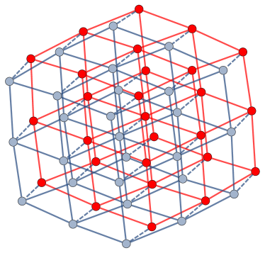
Figure 1: Two-channel 3D Anderson lattice (with $L=3$). An ordered system is coupled to a fully disordered one via $U$ (dashed edges). The latter features on-site potentials $\epsilon_{i}$ falling randomly within $[-W/2,W/2]$ [say, red (dark) vertices]. Here, we set the intra-lattice couplings (solid edges) to $t\equiv 1$. Note that the full Hilbert space is $2N$-dimensional, with $N=L^{3}$.

The Hamiltonian describing a single particle (e.g. an electron) hopping through a 3D bilayered lattice, with $N=L^{3}$ sites each, reads $\hat{H}=\hat{H}_{1}+\hat{H}_{2}+\hat{H}_{I}$, where

$$\hat{H}_{\ell}=\sum_{i}\epsilon_{\ell,i}\hat{c}_{\ell,i}^{\dagger}\hat{c}_{\ell,i}+t\sum_{\langle i,j\rangle}\left(\hat{c}_{\ell,i}^{\dagger}\hat{c}_{\ell,j}+\mathrm{H.c.}\right)$$ (1)

is the local tight-binding Hamiltonian for each layer ($\ell=1,2$), with $t$ and $\epsilon_{\ell,i}$ being, respectively, the intra-hopping strength and the on-site potential, and $\hat{c}_{\ell,i}$ ($\hat{c}_{\ell,i}^{\dagger}$) denoting the fermionic annihilation (creation) operator at site $i$ of the $\ell$-th layer. The sum in the second term of Eq. (1) runs over nearest-neighbors sites of a simple cubic lattice. The coupling between both channels is accounted by

$$\hat{H}_{I}=\sum_{i}U_{i}\left(\hat{c}_{1,i}^{\dagger}\hat{c}_{2,i}+\mathrm{H.c.}\right),$$ (2)

where $U_{i}$ is the inter-layer hopping strength.

At this point, we are to make a few assumptions towards the parameters of the system. First, note that $t$ is constant for both layers, and we set it as our energy unit ($t\equiv 1$). For now, we also set $U_{i}=U$ uniform and assume that one of the layers features no disorder at all, with $\epsilon_{1,i}=0$ whereas $\epsilon_{2,i}$ is taken out of a box distribution within $[-W/2,W/2]$, $W$ being the disorder strength. This configuration is depicted in Fig. 1.

For $U=0$, both layers are decoupled. The ordered one features extended wave functions over the whole the energy spectrum. On the other hand, layer 2 itself is a 3D Anderson model for which a transition between extended and localized states takes place for a given critical value of disorder strength $W_{c}$ that depends on the energy level and lattice topology. For instance, $W_{c}=0$ for 1D and 2D at any energy level, meaning that every eigenstate of the system is exponentially localized even in the presence of the tiniest amount of disorder abrahams79 . For higher dimensions, say, in a simple cubic lattice, the transition is found for $W_{c}/t\approx 16.53$ at the middle of the band ($E=0$) slevin14 . The mobility edge, that is the critical energy above which the particles are free to move has been estimated using ultracold atoms in optical lattices semeghini15 .

III Localization properties

Hereafter we are interested in the case $U\neq 0$. Were both layers ordered (say, setting $\epsilon_{2,i}=0$ as well), things would be straightforward to deal with. In this particular scenario, the Hamiltonian can be handled out analytically in Fourier space, that is $\hat{H}|\psi_{\vec{k},\sigma}\rangle=E_{\vec{k},\sigma}|\psi_{\vec{k},\sigma}\rangle$ where the eigenvalues are

$$E_{\vec{k},\sigma}=\sigma U+\frac{1}{N}\sum_{\langle i,j\rangle}e^{i\vec{k}\cdot(\vec{R}_{i}-\vec{R}_{j})},$$ (3)

$\sigma=\pm 1$, $\vec{R}_{i}$ is the position vector of the $i$-th vertice in the lattice, and $\vec{k}$ is the reciprocal lattice vector satisfying $\vec{k}\cdot\vec{R}_{i}=2\pi n$, where $n$ is an integer. The eigenvectors are

$$|\psi_{\vec{k},\sigma}\rangle=\frac{1}{2N}\sum_{i=1}^{N}e^{i\vec{k}\cdot\vec{R}_{i}}\left(\hat{c}_{1,i}^{{\dagger}}+\sigma\hat{c}_{2,i}^{{\dagger}}\right)|\emptyset\rangle,$$ (4)

with $|\emptyset\rangle$ being the vacuum state and $|i\rangle_{\ell}=\hat{c}_{\ell,i}^{{\dagger}}|\emptyset\rangle$ denoting a single particle located at the $i$-th site of the $\ell$-th channel. Given Eq. (4) it is readily seen that for any eigenstate the probability of finding the particle at a given location is $1/2N$, due to the extended character of the Bloch wavefunctions.

Basically, when linking up two identical ordered systems like discussed above, one gets two effective uncoupled lattices, with local energies $+U$ and $-U$, respectively, and featuring the same dispersion profile [see Eq. (3)]. The states that form those effective structures are even symmetric and anti-symmetric combinations of $|i\rangle_{1}$ and $|i\rangle_{2}$, and then there are two bands of propagating modes at our disposal. At the end of this paper, we show that a band of extended states can be activated even when we couple two disordered lattices, as long as their parameters obey a certain class of correlations.

Our main goal now is to see about how the coupling between the ordered ($\epsilon_{1,i}=0$) and disordered ($\epsilon_{2,i}\in[-W/2,W/2]$) lattices affects the localization-delocalization transition of the full system. At a first glance, we are led to think that the channels may push each other out, meaning that transport in the ordered (disordered) lattice is suppressed (enhanced). At least, that is the outcome for a 1D ladder chain in the case of uncorrelated disorder zhang10 . Here, however, things should get more involved as the 3D Anderson model features mobility edges. To get into further details regarding our bilayered 3D model, we will resort to exact numerical diagonalization of the Hamiltonian in order to obtain the quantities of interest.

Let $|\psi_{k}\rangle=\sum_{i=1}^{N}\left(a_{k,i}|i\rangle_{1}+b_{k,i}|i\rangle_{2}\right)$ be the eigenstate associated to level $E_{k}$. Thus, the probability to find the particle in lattice 1 (lattice 2), that is the ordered (disordered) channel, for a given energy level, is given by $P_{1}(E_{k})=\sum_{i}|a_{k,i}|^{2}$ ($P_{2}(E_{k})=\sum_{i}|b_{k,i}|^{2}$). Observe that $P_{1}(E_{k})+P_{2}(E_{k})=1$. The degree of localization can be characterized through the participation ratio, here defined as

$$R_{1}(E_{k}) =\frac{P_{1}(E_{k})}{\sum_{i=1}^{N}|a_{k,i}|^{4}},$$ (5)

$$R_{2}(E_{k}) =\frac{P_{2}(E_{k})}{\sum_{i=1}^{N}|b_{k,i}|^{4}}.$$ (6)

A localized eigenstate is characterized by $R_{\ell}(E_{k})/N\rightarrow 0$ in the limit $N\rightarrow\infty$ and the ratio converges to a finite value if the the state happens to be extended. In what follows, the energy band is divided into twenty intervals, $(\mathrm{max}\{E_{k}\}-\mathrm{min}\{E_{k}\})/20$, so that the quantities $P_{\ell}(E)$ and $R_{\ell}(E)$ are averages taken over the states allocated within a small window around $E$. We further average them out over $m$ independent samples for each chosen values of $L$, $U$, and $W$.

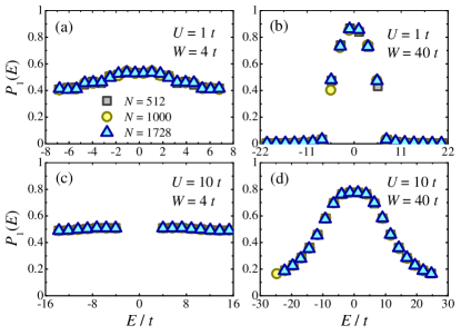
Figure 2: Probability of finding the particle at lattice 1 (ordered), $P_{1}(E)$, averaged over a set of eigenstates surrounding $E$ for (a,b) $U=1t$ and (c,d) $U=10t$, with disorder strengths $W=4t$ and $W=40t$ in each case. Results are obtained for lattice sizes $N=512$ ($L=8$), $N=1000$ ($L=10$), and $N=1728$ ($L=12$), averaged over $m=40$, $20$, and $12$ independent realizations of disorder, respectively.

We start off discussing the overall occupation probability for one of the lattices, say $P_{1}(E)$, accounting for the ordered channel. Results are shown in Fig. 2 for $U=1t$ and $U=10t$, considering two disorder strengths and different system sizes $N$. From Eq. (4), valid for $U\neq 0$ and $W=0$, we get the idea that in the weak disorder regime ($W\ll U$) there should still be likely to find the particle in any of the channels with almost equal probability. Already for $W=4t$, though, and interchannel hopping strength $U=1t$, one starts noticing that the outskirts of the band become slightly less involved with the ordered channel [see Fig. 2(a)]. This reaches a serious level in the presence of intense disorder [Fig. 2(b)] to the point the very center of the band is almost entirely populated by the ordered lattice whilst the disordered counterpart dominates for higher energies (in absolute values), as imposed by $W$. In other words, the eigenstates tend to be no longer mixed upon increasing $W$, except for those lying in between as we depart from the middle of the band. In general, those properties above still stand for higher hopping strengths, as displayed in Fig. 2 for $U=10t$. However, note in Fig. 2(c) that there is an energy gap as $U$ mixes the channels up a great deal and pushes two subbands apart [cf. Eq. (3)]. When $W$ is increased [Fig. 2(d)], the gap is closed as eigenstates featuring higher overlaps with the ordered channel once again move to the center of the band, although the probability distribution over $E$ is not so as sharp as we have seen in Fig. 2(b) due to the value of $U$. We also mention that all those properties are valid regardless of the system size $2N=2L^{3}$.

The above analysis, while revealing some interesting aspects over the population mixedness of the eigenstates in relation to the coupling between ordered and disordered lattices, does not really tell about their localization strength. To do so, we must proceed with a finite-size scaling analysis for the participation ratio. Considering that $R_{\ell}(E_{k})\sim N^{\alpha}$, with $\alpha\in[0,1]$, the state is said to be completely delocalized when $\alpha=1$ and localized otherwise. (One should bear in mind that it is still possible to find several localization profiles for the wavefunctions in that region.)

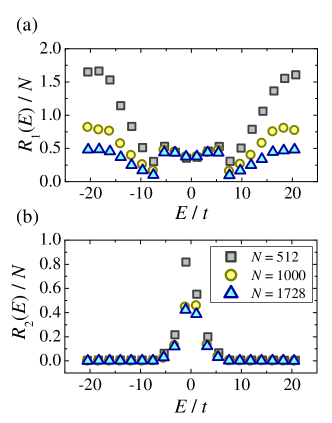
Figure 3: Rescaled participation ratios (a) $R_{1}(E)/N$ (ordered channel) and (b) $R_{2}(E)/N$ (disordered channel) averaged over a set of eigenstates surrounding $E$ for $U=1t$ and $W=40t$. Once again, results are shown for lattice sizes $N=512$ ($L=8$), $N=1000$ ($L=10$), and $N=1728$ ($L=12$), averaged over $m=40$, $20$, and $12$ independent realizations of disorder, respectively.

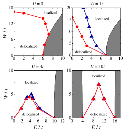
Figure 4: Localization-delocalization phase diagrams for (ordered) channel 1 (blue triangles) and (disordered) channel 2 (red circles) for $U/t=0,1,4,$ and $10$ evaluated via finite-size scaling analysis of $R_{1}(E)$ and $R_{2}(E)$ for $N=512,1000,$ and $1728$ (averaged over $m=40$, $20$, and $12$ samples, respectively). Gray-shaded areas stand for band gaps. Lines are for guiding the eye.

As an example, in Fig. 3 we display the one-lattice participation ratio (divided by $N$), as defined in Eqs. (5) and (6) for $U=1$ and strong disorder ($W=40$), what eventually enforces localization for both lattices in the entire spectrum. Therein we have checked that $\alpha<1$ as expected. To extract some information over the degree of localization though, we must look after the value of $R_{\ell}(E_{k})$ itself. Although lattice 1 (the ordered channel 1) is now effectively disordered, its associated coefficients $\{a_{k,i}\}$ are such that they combine to form a set of localized states featuring a much larger localization length than those associated to lattice 2 in the outskirts of the band [where channel 2 dominates (cf. Fig. 2(b))]. In that region, we checked that the corresponding $\alpha$ is close to zero for both lattices.

We then used the above criteria for the participation ratio to construct the $W-E$ phase diagrams shown in Fig. 4. In the absence of interchannel coupling ($U=0$), we recover the standard phase diagram for the 3D Anderson model (which is lattice 2, only) featuring a critical disorder strength $W_{c}/t$ of about 16.5 at $E=0$, above which the system is localized. But then as we set $U/t=1$ thereby connecting lattices 1 and 2, the latter becomes more sensitive to disorder as the reentrant pattern is gone. A localization-delocalization transition is also induced in in channel 1 (hitherto ordered) for higher values of $W_{c}$. For intermediate values of $W_{c}$, although the wavefunction components of lattice 2 suggests a localized phase, lattice 1 still holds the system in the delocalized phase, especially for energies around the band center, filled out with eigenstates mostly overlapping with the ordered channel. Both channels happen to feature about the same behavior when $U/t=4$ due to the band mixing leading to low values of critical disorder strength overall. For $U/t=10$, the coupling between both lattices is such that one can barely tell them apart. Each subband [notice the gap taking place around the middle of the spectrum; see Fig. 2(c)] features a transition around $W_{c}/t=7$ at its center. In this strong-$U$ regime each channel, on its own, is thus able to provide valuable information over the whole lattice.

IV Disorder-free subspace

So far we have been dealing with the localization properties of a disordered 3D lattice coupled to a ordered one. In this last section, though, we consider both lattices to feature on-site disorder and show analytically, following Ref. sil08prb , that certain correlations among parameters $\epsilon_{1,i}$, $\epsilon_{2,i}$, and $U_{i}$ [cf. Eqs. (1) and (2)] can effectively decouple both channels, thereby spanning a disorder-free subspace. In the following procedure, the intra-lattice hopping strength $t\equiv 1$, still.

Each (two-level-like) cell formed from states $|i\rangle_{1}$ and $|i\rangle_{2}$ features the local Hamiltonian

$$H_{i}^{(\mathrm{cell})}=\begin{pmatrix}\epsilon_{1,i}&U_{i}\\ U_{i}&\epsilon_{2,i}\end{pmatrix},$$ (7)

which can be put in diagonal form via

$$|+\rangle_{i} =\sin\theta_{i}|i\rangle_{1}+\cos\theta_{i}|i\rangle_{2},$$ (8)

$$|-\rangle_{i} =\cos\theta_{i}|i\rangle_{1}-\sin\theta_{i}|i\rangle_{2},$$ (9)

with correponding eigenvalues

$$E_{i}^{\pm}=\frac{1}{2}\left(\epsilon_{1,i}+\epsilon_{2,i}\pm\sqrt{4U_{i}^{2}+\Delta_{i}^{2}}\right),$$ (10)

where $\Delta_{i}=\epsilon_{2,i}-\epsilon_{1,i}$ is the local energy detuning and

$$\theta_{i}=\tan^{-1}\left(\frac{2U_{i}}{\sqrt{4U_{i}^{2}+\Delta_{i}^{2}}+\Delta_{i}}\right).$$ (11)

Rewriting the system Hamiltonian in terms of operators $\alpha_{i}^{(\mu)\dagger}\equiv|\mu\rangle_{i}\langle\emptyset|$ $(i=1,\ldots,N)$, with $\mu=\pm$, we get

$$H= \sum_{i,\mu}E_{i}^{\mu}\alpha_{i}^{(\mu)\dagger}\alpha_{i}^{(\mu)}+\sum_{\langle i,j\rangle,\mu}J_{ij}^{(\mathrm{intra})}\left(\alpha_{i}^{(\mu)\dagger}\alpha_{j}^{(\mu)}+\mathrm{H.c.}\right)$$

$$+\sum_{\langle i,j\rangle}J_{ij}^{(\mathrm{inter})}\left(\alpha_{i}^{(+)\dagger}\alpha_{j}^{(-)}+\mathrm{H.c.}\right),$$ (12)

where

$$J_{ij}^{(\mathrm{intra})} =t\cos(\theta_{i}-\theta_{j}),$$ (13)

$$J_{ij}^{(\mathrm{inter})} =t\sin(\theta_{i}-\theta_{j}).$$ (14)

The above description keeps the intraconnectivity pattern of each subsystem while establishes more interconnections per (effective) site.

If we want one of the channels – that is the positive or the negative branch – to be free of (diagonal) disorder, the first step is to place all of its local energies at the same level, say, zero for simplicity. Then, given $U_{i}=\pm\sqrt{\epsilon_{1,i}\epsilon_{2,i}}$ (with $\epsilon_{1,i},\epsilon_{2,i}>0$) one has $E_{i}^{+}=\epsilon_{1,i}+\epsilon_{2,i}$ and $E_{i}^{-}=0$ for all $i$ [see Eq. (10)]. In this case, we arrive at a similar situation as before, where a disordered lattice (positive branch) is coupled to a ordered one (negative branch). Then, we further need to decouple them, by arranging for $J_{ij}^{(\mathrm{inter})}=0$, what implies that $\theta_{i}-\theta_{j}=n\pi$ for any integer $n$. From Eq. (11) we thus see that $\tan\theta_{i}=\tan\theta_{j}$ for all $i$ and $j$. As, given $U_{i}=\sqrt{\epsilon_{1,i}\epsilon_{2,i}}$ (with no loss of generality), $\tan\theta_{i}=2\sqrt{\epsilon_{1,i}/\epsilon_{2,i}}$, it is then required that $\epsilon_{2,i}/\epsilon_{1,i}=\epsilon$, what makes $U_{i}/\epsilon_{1,i}=\sqrt{\epsilon}$, with fixed $\epsilon>0$ over the entire lattice sil08prb . This set of correlations entails $J_{ij}^{(\mathrm{intra})}=t$ and, finally, we obtain two independent effective lattices, a clean one and another featuring on-site disorder with $E_{i}^{+}=\epsilon_{1,i}(1+\epsilon)$, for which results of Anderson localization theory in 3D are known.

V Conclusions

We explored the localization-delocalization transition in a bilayered (two-channel) Anderson model in three dimensions. First we considered one of the lattices being ordered, with the other one featuring diagonal uncorrelated disorder, and discussed about the role of their coupling upon the mobility edges of each channel separately, evaluated through the participation ratio. In summary, for moderate interchannel coupling the ordered channel begins to feature effective on-site fluctuations leading to relatively weak disorder when compared to the other (already disordered) channel. Strong coupling leads to mixing between both channels and they thus happen to feature almost the same critical disorder strengths along the spectrum.

Following that, we also considered two coupled disordered 3D lattices and showed how to create an effective channel completely free of disorder. The very coexistence between localized and delocalized states that emerges from the above and similar frameworks provides with the idea of engineering extended states in a disordered background hilke03 ; sil08prb ; rodriguez12 ; guo13 ; almeida18DFS . While individual chains with correlated disorder already offers a great deal of selective transport properties – that can be used, for instance, in entanglement distribution almeida17pra ; almeida19qip and quantum-state transfer almeida18ann ; junior19 protocols – laterally-coupled channels add more possibilities, given the strength of the interchain hopping as it is able to mix modes with totally different profiles.

To some extent, this work was also motivated by the fact that recent advances in ultracold atoms in optical lattices have reached higher levels of local control gross17 , not to mention such platforms had already had success in probing Anderson localization phenomenon in 3D kondov11 ; jendrzejewski12 ; semeghini15 . Further extensions of our work should include non-trivial topologies, such as complex networks with small-world characteristics for they display remarkable localization properties zhu00 ; giraud05 ; cardoso08 . It would thus be interesting to see about how concatenating many channels made up of those affects the dynamical properties of the whole system and evaluate its robustness against disorder and other kinds of noise.

References

- (1) P. W. Anderson, Phys. Rev. 109, 1492 (1958).
- (2) F. Evers and A. D. Mirlin, Rev. Mod. Phys. 80, 1355 (2008).
- (3) E. Abrahams, P. W. Anderson, D. C. Licciardello, and T. V. Ramakrishnan, Phys. Rev. Lett. 42, 673 (1979).
- (4) S. S. Kondov, W. R. McGehee, J. J. Zirbel, and B. DeMarco, Science 334, 66 (2011).
- (5) F. Jendrzejewski et al., Nat. Phys. 8, 398 (2012).
- (6) G. Semeghini et al., Nat. Phys. 11, 554 (2015).
- (7) J. C. Flores, J. Phys. Condens. Matter 1, 8471 (1989).
- (8) D. H. Dunlap, H.-L. Wu, and P. W. Phillips, Phys. Rev. Lett. 65, 88 (1990).
- (9) F. A. B. F. de Moura and M. L. Lyra, Phys. Rev. Lett. 81, 3735 (1998).
- (10) F. M. Izrailev and A. A. Krokhin, Phys. Rev. Lett. 82, 4062 (1999).
- (11) M. Hilke, Phys. Rev. Lett. 91, 226403 (2003).
- (12) A. M. C. Souza and R. F. S. Andrade, Physica A 525, 628 (2019).
- (13) J. Heinrichs, Phys. Rev. B 66, 155434 (2002).
- (14) J. Heinrichs, Phys. Rev. B 68, 155403 (2003).
- (15) R. A. Römer and H. Schulz-Baldes, Europhys. Lett. 68, 247 (2004).
- (16) T. Sedrakyan and A. Ossipov Phys. Rev. B 70, 214206 (2004).
- (17) R. A. Roemer and M. S. Turner, Biophys. J. 89, 2187 (2005).
- (18) E. Díaz, A. Sedrakyan, D. Sedrakyan, and F. Domínguez-Adame Phys. Rev. B 75, 014201 (2007)
- (19) V. M. K. Bagci and A. A. Krokhin Phys. Rev. B 76, 134202 (2007)
- (20) S. Sil, S. K. Maiti, and A. Chakrabarti, Phys. Rev. Lett. 101, 076803 (2008).
- (21) S. Sil, S. K. Maiti, and A. Chakrabarti, Phys. Rev. B 78, 113103 (2008).
- (22) F. A. B. F. de Moura, R. A. Caetano, and M. L. Lyra, Phys. Rev. B 81, 125104 (2010).
- (23) W. Zhang, R. Yang, Y. Zhao, S. Duan, P. Zhang, and S. E. Ulloa, Phys. Rev. B 81, 214202 (2010).
- (24) A.-M. Guo and S.-J. Xiong, Phys, Rev. B 83, 245108 (2011).
- (25) A. Rodriguez, A. Chakrabarti, and R. A. Römer, Phys. Rev. B 86 085119 (2012).
- (26) H. Y. Xie, V. E. Kravtsov, and M. Müller, Phys. Rev. B 86, 014205 (2012).
- (27) B. P. Nguyen and K. Kim, J. Phys.: Condens. Matter 24, 135303 (2012).
- (28) Y. Zhao, S. Duan, and W. Zhang, J. Phys.: Condens. Matter 24, 245502 (2012).
- (29) A.-M. Guo, S.-J. Xiong, X. C. Xie, and Q.-f. Sun, J. Phys.: Condens. Matter 25, 415501 (2013).
- (30) D. Weinmann and S. N. Evangelou, Phys. Rev. B 90, 155411 (2014).
- (31) P. Bordia, H. P. Luschen, S. S. Hodgman, M. Schreiber, I. Bloch, and U. Schneider, Phys. Rev. Lett. 116, 140401 (2016).
- (32) V. Mastropietro, Phys. Rev. B 95, 075155 (2017).
- (33) Y. Zhao, S. Ahmed, and J. Sirker, Phys. Rev. B 95, 235152 (2017).
- (34) G. M. A. Almeida, A. M. C. Souza, F. A. B. F. de Moura, and M. L. Lyra, Phys. Lett A 383, 125847 (2019).
- (35) Y. Asada, K. Slevin, and T. Ohtsuki, Phys. Rev. Lett. 89, 256601 (2002).
- (36) S. Hikami, A. I. Larkin, and Y. Nagaoka, Prog. Theor. Phys. 63, 707 (1980).
- (37) S. N. Evangelou and T. Ziman, J. Phys. C 20, L235 (1987).
- (38) T. Ando, Phys. Rev. B 40, 5325 (1989).
- (39) R. Merkt, M. Janssen, and B. Huckestein, Phys. Rev. B 58, 4394 (1998).
- (40) G. Orso, Phys. Rev. Lett. 118, 105301 (2017).
- (41) Ying Su and X. R. Wang, Phys. Rev. B 98, 224204 (2018).
- (42) L. Zhou, H. Pu, and W. Zhang, Phys. Rev. A 87, 023625 (2013).
- (43) L. Huang, Z. Meng, P. Wang, P. Peng, S.-L. Zhang, L. Chen, D. Li, Q. Zhou, and J. Zhang, Nat. Phys. 12, 540 (2016).
- (44) K. Slevin and T. Ohtsuki, New J. Phys. 16, 015012 (2014).
- (45) G. M. A. Almeida, F. A. B. F. de Moura, T. J. G. Apollaro, and M. L. Lyra, Phys. Rev. A 96, 032315 (2017).
- (46) G. M. A. Almeida, F. A. B. F. de Moura, and M. L. Lyra, Quant. Inf. Proc. 18, 41 (2019).
- (47) G. M. A. Almeida, C. V. C. Mendes, M. L. Lyra, F. A. B. F. de Moura, Ann. Phys. 398, 180 (2018).
- (48) P. R. S. Júnior, G. M. A. Almeida, M. L. Lyra, and F. A. B. F. de Moura, Phys. Lett. A 383, 1845 (2019).
- (49) C. Gross and I. Bloch, Science 357, 995 (2017).
- (50) C.-P. Zhu and S.-J Xiong, Phys. Rev. B 62, 14780 (2000).
- (51) O. Giraud, B. Georgeot, and D. L. Shepelyansky, Phys Rev. E 72, 036203 (2005).
- (52) A. L. Cardoso, R. F. S. Andrade, and A. M. C. Souza, Phys. Rev. B 78, 214202 (2008).