A Distributed Quasi-Newton Algorithm for Primal and Dual Regularized Empirical Risk Minimization

Abstract

We propose a communication- and computation-efficient distributed optimization algorithm using second-order information for solving empirical risk minimization (ERM) problems with a nonsmooth regularization term. Our algorithm is applicable to both the primal and the dual ERM problem. Current second-order and quasi-Newton methods for this problem either do not work well in the distributed setting or work only for specific regularizers. Our algorithm uses successive quadratic approximations of the smooth part, and we describe how to maintain an approximation of the (generalized) Hessian and solve subproblems efficiently in a distributed manner. When applied to the distributed dual ERM problem, unlike state of the art that takes only the block-diagonal part of the Hessian, our approach is able to utilize global curvature information and is thus magnitudes faster. The proposed method enjoys global linear convergence for a broad range of non-strongly convex problems that includes the most commonly used ERMs, thus requiring lower communication complexity. It also converges on non-convex problems, so has the potential to be used on applications such as deep learning. Computational results demonstrate that our method significantly improves on communication cost and running time over the current state-of-the-art methods.

1 Introduction

We consider using multiple machines to solve the following regularized problem

$$\min_{{\boldsymbol{w}}\in\mathbb{R}^{d}}\quad P\left({\boldsymbol{w}}\right)\coloneqq\xi\left(X^{\top}{\boldsymbol{w}}\right)+g\left({\boldsymbol{w}}\right),$$ (1)

where $X$ is a $d$ by $n$ real-valued matrix, and $g$ is a convex, closed, and extended-valued proper function that can be nondifferentiable, or its dual problem

$$\min_{{\boldsymbol{\alpha}}\in\mathbb{R}^{n}}\quad D\left({\boldsymbol{\alpha}}\right)\coloneqq g^{*}\left(X{\boldsymbol{\alpha}}\right)+\xi^{*}\left(-{\boldsymbol{\alpha}}\right),$$ (2)

where for any given function $f(\cdot)$, $f^{*}$ denotes its convex conjugate

$$f^{*}\left(z\right)\coloneqq\max_{y}\quad z^{\top}y-f\left(y\right).$$

Each column of $X$ represents a single data point or instance, and we assume that the set of data points is partitioned and spread across $K>1$ machines (i.e. distributed instance-wise). We write $X$ as

$$X\coloneqq\left[X_{1},X_{2},\dotsc,X_{K}\right]$$ (3)

where $X_{k}$ is stored exclusively on the $k$th machine. The dual variable ${\boldsymbol{\alpha}}$ is formed by concatenating ${\boldsymbol{\alpha}}_{1},{\boldsymbol{\alpha}}_{2},\dotsc,{\boldsymbol{\alpha}}_{K}$ where ${\boldsymbol{\alpha}}_{k}$ is the dual variable corresponding to $X_{k}$. We let $\mathcal{I}^{X}_{1},\dotsc,\mathcal{I}^{X}_{K}$ denote the indices of the columns of $X$ corresponding to each of the $X_{k}$ matrices. We further assume that $\xi$ shares the same block-separable structure and can be written as follows:

$$\xi\left(X^{\top}{\boldsymbol{w}}\right)=\sum_{k=1}^{K}\xi_{k}\left(X_{k}^{\top}{\boldsymbol{w}}\right),$$ (4)

and therefore in (2), we have

$$\xi^{*}\left(-{\boldsymbol{\alpha}}\right)=\sum_{k=1}^{K}\xi^{*}_{k}\left(-{\boldsymbol{\alpha}}_{k}\right).$$ (5)

For the ease of description and unification, when solving the primal problem, we also assume that there exists some partition $\mathcal{I}^{g}_{1},\dotsc,\mathcal{I}^{g}_{K}$ of $\{1,\dotsc,d\}$ and $g$ is block-separable according to the partition:

$$g\left({\boldsymbol{w}}\right)=\sum_{k=1}^{K}g_{k}\left({\boldsymbol{w}}_{\mathcal{I}^{g}_{k}}\right),$$ (6)

though our algorithm can be adapted for non-separable $g$ with minimal modification, see the preliminary version Lee et al. (2018).

When we solve the primal problem (1), $\xi$ is assumed to be a differentiable function with Lipschitz continuous gradients, and is allowed to be nonconvex. On the other hand, when the dual problem (2) is considered, for recovering the primal solution, we require strong convexity on $g$ and convexity on $\xi$, and $\xi$ can be either nonsmooth but Lipschitz continuous (within the area of interest), or Lipschitz continuously differentiable. Note that strong convexity of $g$ implies that $g^{*}$ is Lipschitz-continuously differentiable (Hiriart-Urruty and Lemaréchal, 2001, Part E, Theorem 4.2.1 and Theorem 4.2.2), making (2) have the same structure as (1) such that both problems have one smooth and one nonsmooth term. There are several reasons for considering the alternative dual problem. First, when $\xi$ is nonsmooth, the primal problem becomes hard to solve as both terms are nonsmooth, meanwhile in the dual problem, $\xi^{*}$ is guaranteed to be smooth. Second, the number of variables in the primal and the dual problem are different. In our algorithm whose spatial and temporal costs are positively correlated to the number of variables, when the data set has much higher feature dimension than the number of data points, solving the dual problem can be more economical.

The bottleneck in performing distributed optimization is often the high cost of communication between machines. For (1) or (2), the time required to retrieve $X_{k}$ over a network can greatly exceed the time needed to compute $\xi_{k}$ or its gradient with locally stored $X_{k}$. Moreover, we incur a delay at the beginning of each round of communication due to the overhead of establishing connections between machines. This latency prevents many efficient single-core algorithms such as coordinate descent (CD) and stochastic gradient and their asynchronous parallel variants from being employed in large-scale distributed computing setups. Thus, a key aim of algorithm design for distributed optimization is to improve the communication efficiency while keeping the computational cost affordable. Batch methods are preferred in this context, because fewer rounds of communication occur in distributed batch methods.

When the objective is smooth, many batch methods can be used directly in distributed environments to optimize them. For example, Nesterov’s accelerated gradient (AG) (Nesterov, 1983) enjoys low iteration complexity, and since each iteration of AG only requires one round of communication to compute the new gradient, it also has good communication complexity. Although its supporting theory is not particularly strong, the limited-memory BFGS (LBFGS) method (Liu and Nocedal, 1989) is popular among practitioners of distributed optimization. It is the default algorithm for solving $\ell_{2}$-regularized smooth ERM problems in Apache Spark’s distributed machine learning library (Meng et al., 2016), as it is empirically much faster than AG (see, for example, the experiments in Wang et al. (2019)). Other batch methods that utilize the Hessian of the objective in various ways are also communication-efficient under their own additional assumptions (Shamir et al., 2014; Zhang and Lin, 2015; Lee et al., 2017; Zhuang et al., 2015; Lin et al., 2014).

However, when the objective is nondifferentiable, neither LBFGS nor Newton’s method can be applied directly. Leveraging curvature information from the smooth part ($\xi$ in the primal or $g^{*}$ in the dual) can still be beneficial in this setting. For example, the orthant-wise quasi-Newton method OWLQN (Andrew and Gao, 2007) adapts the LBFGS algorithm to the special nonsmooth case in which $g(\cdot)\equiv\|\cdot\|_{1}$ for (1), and is popular for distributed optimization of $\ell_{1}$-regularized ERM problems. Unfortunately, extension of this approach to other nonsmooth $g$ is not well understood, and the convergence guarantees are only asymptotic, rather than global. Another example is that for (2), state of the art distributed algorithms (Yang, 2013; Lee and Chang, 2019; Zheng et al., 2017) utilize block-diagonal entries of the real Hessian of $g^{*}(X{\boldsymbol{\alpha}})$.

To the best of our knowledge, for ERMs with general nonsmooth regularizers in the instance-wise storage setting, proximal-gradient-like methods (Wright et al., 2009; Beck and Teboulle, 2009; Nesterov, 2013) are the only practical distributed optimization algorithms with convergence guarantees for the primal problem (1). Since these methods barely use the curvature information of the smooth part (if at all), we suspect that proper utilization of second-order information has the potential to improve convergence speed and therefore communication efficiency dramatically. As for algorithms solving the dual problem (2), computing $X{\boldsymbol{\alpha}}$ in the instance-wise storage setting requires communicating a $d$-dimensional vector, and only the block-diagonal part of $\partial^{2}_{{\boldsymbol{\alpha}}}g^{*}(X{\boldsymbol{\alpha}})$ can be obtained easily. Therefore, global curvature information is not utilized in existing algorithms, and we expect that utilizing global second-order information of $g^{*}$ can also provide substantial benefits over the block-diagonal approximation approaches. We thus propose a practical distributed inexact variable-metric algorithm that can be applied to both (1) and (2). Our algorithm uses gradients and updates information from previous iterations to estimate curvature of the smooth part in a communication-efficient manner. We describe construction of this estimate and solution of the corresponding subproblem. We also provide convergence rate guarantees, which also bound communication complexity. These rates improve on existing distributed methods, even those tailor-made for specific regularizers.

More specifically, We propose a distributed inexact proximal-quasi-Newton-like algorithm that can be used to solve both (1) and (2) under the instance-wise split setting that share the common structure of having a smooth term $f$ and a nonsmooth term $\Psi$. At each iteration with the current iterate $x$, our algorithm utilizes the previous update directions and gradients to construct a second-order approximation of the smooth part $f$ by the LBFGS method, and approximately minimizes this quadratic term plus the nonsmooth term $\Psi$ to obtain an update iteration $p$.

$$p\approx\arg\min_{p}\,Q_{H}(p;x),$$ (7)

where $H$ is the LBFGS approximation of the Hessian of $f$ at $x$, and

$$Q_{H}(p;x)\coloneqq\nabla f(x)^{\top}p+\frac{1}{2}p^{\top}Hp+\Psi(x+p)-\Psi(x).$$ (8)

For the primal problem (1), we believe that this work is the first to propose, analyze, and implement a practically feasible distributed optimization method for solving (1) with general nonsmooth regularizer $g$ under the instance-wise storage setting. For the dual problem (2), our algorithm is the first to suggest an approach that utilizes global curvature information under the constraint of distributed data storage. This usage of non-local curvature information greatly improves upon state of the art for the distributed dual ERM problem which uses the block-diagonal parts of the Hessian only. An obvious drawback of the block-diagonal approach is that the convergence deteriorates with the number of machines, as more and more off-block-diagonal entries are ignored. In the extreme case, where there are $n$ machines such that each machine stores only one column of $X$, the block-diagonal approach reduces to a scaled proximal-gradient algorithm and the convergence is expected to be extremely slow. On the other hand, our algorithm has convergence behavior independent of number of machines and data distribution over nodes, and is thus favorable when many machines are used. Our approach has both good communication and computational complexities, unlike certain approaches that focus only on communication at the expense of computation (and ultimately overall time).

1.1 Contributions

We summarize our main contributions as follows.

• The proposed method is the first real distributed second-order method for the dual ERM problem that utilizes global curvature information of the smooth part. Existing second-order methods use only the block-diagonal part of the Hessian and suffers from asymptotic convergence speed as slow as proximal gradient, while our method enjoys fast convergence throughout. Numerical results show that our inexact proximal-quasi-Newton method is magnitudes faster than state of the art for distributed optimizing the dual ERM problem.

• We propose the first distributed algorithm for primal ERMs with general nonsmooth regularizers (1) under the instance-wise split setting. Prior to our work, existing algorithms are either for a specific regularizer (in particular the $\ell_{1}$ norm) or for the feature-wise split setting, which is often impractical. In particular, it is usually easier to generate new data points than to generate new features, and each time new data points are obtained from one location, one needs to distribute their entries to different machines under the feature-wise setting.

• The proposed framework is applicable to both primal and dual ERM problems under the same instance-wise split setting, and the convergence speed is not deteriorated by the number of machines. Existing methods that applicable to both problems can deal with feature-wise split for the primal problem only, and their convergence degrades with the number of machines used, and are thus not suitable for large-scale applications where thousands of or more machines are used. This unification also reduces two problems into one and facilitates future development for them.

• Our analysis provides sharper convergence guarantees and therefore better communication efficiency. In particular, global linear convergence for a broad class of non-strongly convex problems that includes many popular ERM problems are shown, and an early linear convergence to rapidly reach a medium solution accuracy is proven for convex problems.

1.2 Organization

We first describe the general distributed algorithm in Section 2. Convergence guarantee, communication complexity, and the effect of the subproblem solution inexactness are analyzed in Section 3. Specific details for applying our algorithm respectively on the primal and the dual problem are given in Section 4. Section 5 discusses related works, and empirical comparisons are conducted in Section 6. Concluding observations appear in Section 7.

1.3 Notation and Assumptions

We use the following notation.

• $\|\cdot\|$ denotes the 2-norm, both for vectors and for matrices.

• Given any symmetric positive semi-definite matrix $H\in\mathbb{R}^{d\times d}$ and any vector $p\in\mathbb{R}^{d}$, $\|p\|_{H}$ denotes the semi-norm $\sqrt{p^{\top}Hp}$.

In addition to the structural assumptions of distributed instance-wise storage of $X$ in (3) and the block separability of $\xi$ in (4), we also use the following assumptions throughout this work. When we solve the primal problem, we assume the following.

Assumption 1

The regularization term $g({\boldsymbol{w}})$ is convex, extended-valued, proper, and closed. The loss function $\xi(X^{\top}{\boldsymbol{w}})$ is $L$-Lipschitz continuously differentiable with respect to ${\boldsymbol{w}}$ for some $L>0$. That is,

$$\left\|X^{\top}\xi^{\prime}\left(X^{\top}{\boldsymbol{w}}_{1}\right)-X^{\top}\xi^{\prime}\left(X^{\top}{\boldsymbol{w}}_{2}\right)\right\|\leq L\left\|{\boldsymbol{w}}_{1}-{\boldsymbol{w}}_{2}\right\|,\forall{\boldsymbol{w}}_{1},{\boldsymbol{w}}_{2}\in\mathbb{R}^{d}.$$ (9)

On the other hand, when we consider solving the dual problem, the following is assumed.

Assumption 2

Both $g$ and $\xi$ are convex. $g^{*}(X{\boldsymbol{\alpha}})$ is $L$-Lipschitz continuously differentiable with respect to ${\boldsymbol{\alpha}}$. Either $\xi^{*}$ is $\sigma$-strongly convex for some $\sigma>0$, or the loss term $\xi(X^{\top}{\boldsymbol{w}})$ is $\rho$-Lipschitz continuous for some $\rho$.

Because a function is $\rho$-Lipschitz continuously differentiable if and only if its conjugate is $(1/\rho)$-strongly convex (Hiriart-Urruty and Lemaréchal, 2001, Part E, Theorem 4.2.1 and Theorem 4.2.2), Assumption 2 implies that $g$ is $\|X^{\top}X\|/L$-strongly convex. From the same reasoning, $\xi^{*}$ is $\sigma$-strongly convex if only if $\xi$ is $(1/\sigma)$ Lipschitz continuously differentiable. Convexity of the primal problem in Assumption 2 together with Slater’s condition guarantee strong duality Boyd and Vandenberghe (2004, Section 5.2.3), which then ensures (2) is indeed an alternative to (1). Moreover, from KKT conditions, any optimal solution ${\boldsymbol{\alpha}}^{*}$ for (2) gives us a primal optimal solution ${\boldsymbol{w}}^{*}$ for (1) through

$${\boldsymbol{w}}^{*}=\nabla g^{*}(X{\boldsymbol{\alpha}}^{*}).$$ (10)

2 Algorithm

We describe and analyze a general algorithmic scheme that can be applied to solve both the primal (1) and dual (2) problems under the instance-wise distributed data storage scenario (3). In Section 4, we discuss how to efficiently implement particular steps of this scheme for (1) and (2).

Consider a general problem of the form

$$\min_{x\in\mathbb{R}^{N}}\quad F(x)\coloneqq f(x)+\Psi(x),$$ (11)

where $f$ is $L$-Lipschitz continuously differentiable for some $L>0$ and $\Psi$ is convex, closed, proper, extended valued, and block-separable into $K$ blocks. More specifically, we can write $\Psi(x)$ as

$$\Psi(x)=\sum_{k=1}^{K}\Psi_{k}(x_{\mathcal{I}_{k}}).$$ (12)

where $\mathcal{I}_{1},\dotsc,\mathcal{I}_{K}$ partitions $\{1,\dotsc,N\}$.

We assume as well that for the $k$th machine, $\nabla_{\mathcal{I}_{k}}f(x)$ can be obtained easily after communicating a vector of size $O(d)$ across machines, and postpone the detailed gradient calculation until we discuss specific problem structures in later sections. Note that this $d$ is the primal variable dimension in (1) and is independent of $N$.

The primal and dual problems are specific cases of the general form (11). For the primal problem (1) we let $N=d$, $x={\boldsymbol{w}}$, $f(\cdot)=\xi(X^{\top}\cdot)$, and $\Psi(\cdot)=g(\cdot)$. The block-separability of $g$ (6) gives the desired block-separability of $\Psi$ (12), and the Lipschitz-continuous differentiability of $f$ comes from Assumption 1. For the dual problem (2), we have $N=n$, $x={\boldsymbol{\alpha}}$, $f(\cdot)=g^{*}(X\cdot)$, and $\Psi(\cdot)=\xi^{*}(-\cdot)$. The separability follows from (5), where the partition (12) reflects the data partition in (3) and Lipschitz continuity from Assumption 2.

Each iteration of our algorithm has four main steps – (1) computing the gradient $\nabla f(x)$, (2) constructing an approximate Hessian $H$ of $f$, (3) solving a quadratic approximation subproblem to find an update direction $p$, and finally (4) taking a step $x+\lambda p$ either via line search or trust-region approach. The gradient computation step and part of the line search process is dependent on whether we are solving the primal or dual problem, and we defer the details to Section 4. The approximate Hessian $H$ comes from the LBFGS algorithm Liu and Nocedal (1989). To compute the update direction, we approximately solve (7), where $Q_{H}$ consists of a quadratic approximation to $f$ and the regularizer $\Psi$ as defined in (8). We then use either a line search procedure to determine a suitable stepsize $\lambda$ and perform the update $x\leftarrow x+\lambda p$, or use some trust-region-like techniques to decide whether to accept the update direction with unit step size.

We now discuss the following issues in the distributed setting: communication cost in distributed environments, the choice and construction of $H$ that have low cost in terms of both communication and per machine computation, procedures for solving (7), and the line search and trust-region procedures for ensuring sufficient objective decrease.

2.1 Communication Cost Model

For the ease of description, we assume the allreduce model of MPI (Message Passing Interface Forum, 1994) throughout the work, but it is also straightforward to extend the framework to a master-worker platform. Under this allreduce model, all machines simultaneously fulfill master and worker roles, and for any distributed operations that aggregate results from machines, the resultant is broadcast to all machines.

This can be considered as equivalent to conducting one map-reduce operation and then broadcasting the result to all nodes. The communication cost for the allreduce operation on a $d$-dimensional vector under this model is

$$\log\left(K\right)T_{\text{initial}}+dT_{\text{byte}},$$ (13)

where $T_{\text{initial}}$ is the latency to establish connection between machines, and $T_{\text{byte}}$ is the per byte transmission time (see, for example, Chan et al. (2007, Section 6.3)).

The first term in (13) also explains why batch methods are preferable. Even if methods that frequently update the iterates communicate the same amount of bytes, it takes more rounds of communication to transmit the information, and the overhead of $\log(K)T_{\text{initial}}$ incurred at every round of communication makes this cost dominant, especially when $K$ is large.

In subsequent discussion, when an allreduce operation is performed on a vector of dimension $O(d)$, we simply say that a round of $O(d)$ communication is conducted. We omit the latency term since batch methods like ours tend to have only a small constant number of rounds of communication per iteration. By contrast, non-batch methods such as CD or stochastic gradient require number of communication rounds per epoch equal to data size or dimension, and therefore face much more significant latency issues.

2.2 Constructing a good $H$ efficiently

We use the Hessian approximation constructed by the LBFGS algorithm (Liu and Nocedal, 1989) as our $H$ in (8), and propose a way to maintain it efficiently in a distributed setting. In particular, we show that most vectors involved can be stored perfectly in a distributed manner in accord with the partition $\mathcal{I}_{k}$ in (12), and this distributed storage further facilitates parallelization of most computation. Note that the LBFGS algorithm works even if the smooth part is not twice-differentiable, see Lemma 1. In fact, Lipschitz continuity of the gradient implies that the function is twice-differentiable almost everywhere, and generalized Hessian can be used at the points where the smooth part is not twice-differentiable. In this case, the LBFGS approximation is for the generalized Hessian.

Using the compact representation in Byrd et al. (1994), given a prespecified integer $m>0$, at the $t$th iteration for $t>0$, let $m(t)\coloneqq\min(m,t)$, and define

$${\boldsymbol{s}}_{i}\coloneqq x^{i+1}-x^{i},\quad{\boldsymbol{y}}_{i}\coloneqq\nabla f(x^{i+1})-\nabla f(x^{i}),\quad\forall i.$$

The LBFGS Hessian approximation matrix is

$$H_{t}=\gamma_{t}I-U_{t}M_{t}^{-1}U_{t}^{\top},$$ (14)

where

$$U_{t}\coloneqq\left[\gamma_{t}S_{t},Y_{t}\right],\quad M_{t}\coloneqq\left[\begin{array}[]{cc}\gamma_{t}S_{t}^{\top}S_{t},&L_{t}\\ L_{t}^{\top}&-D_{t}\end{array}\right],\quad\gamma_{t}\coloneqq\frac{{\boldsymbol{y}}_{t-1}^{\top}{\boldsymbol{y}}_{t-1}}{{\boldsymbol{s}}_{t-1}^{\top}{\boldsymbol{y}}_{t-1}},$$ (15)

and

$$S_{t} \coloneqq\left[{\boldsymbol{s}}_{t-m(t)},{\boldsymbol{s}}_{t-m(t)+1},\dotsc,{\boldsymbol{s}}_{t-1}\right],$$ (16a)

$$Y_{t} \coloneqq\left[{\boldsymbol{y}}_{t-m(t)},{\boldsymbol{y}}_{t-m(t)+1},\dotsc,{\boldsymbol{y}}_{t-1}\right],$$ (16b)

$$D_{t} \coloneqq\text{diag}\left({\boldsymbol{s}}_{t-m(t)}^{\top}{\boldsymbol{y}}_{t-m(t)},\dotsc,{\boldsymbol{s}}_{t-1}^{\top}{\boldsymbol{y}}_{t-1}\right),$$ (16c)

$$\left(L_{t}\right)_{i,j} \coloneqq\begin{cases}{\boldsymbol{s}}_{t-m(t)-1+i}^{\top}{\boldsymbol{y}}_{t-m(t)-1+j},&\text{ if }i>j,\\ 0,&\text{ otherwise.}\end{cases}$$ (16d)

For $t=0$ where no ${\boldsymbol{s}}_{i}$ and ${\boldsymbol{y}}_{i}$ are available, we either set $H_{0}\coloneqq a_{0}I$ for some positive scalar $a_{0}$, or use some Hessian approximation constructed using local data. More details are given in Section 4 when we discuss the primal and dual problems individually.

If $f$ is not strongly convex, it is possible that (14) is only positive semi-definite, making the subproblem (7) ill-conditioned. In this case, we follow Li and Fukushima (2001), taking the $m$ update pairs to be the most recent $m$ iterations for which the inequality

$${\boldsymbol{s}}_{i}^{\top}{\boldsymbol{y}}_{i}\geq\delta{\boldsymbol{s}}_{i}^{\top}{\boldsymbol{s}}_{i}$$ (17)

is satisfied, for some predefined $\delta>0$. It can be shown that this safeguard ensures that $H_{t}$ are always positive definite and the eigenvalues are bounded within a positive range. For a proof in the case that $f$ is twice-differentiable, see, for example, the appendix of Lee and Wright (2017). For completeness, we provide a proof without the assumption of twice-differentiability of $f$ in Lemma 1.

To construct and utilize this $H_{t}$ efficiently, we store $(U_{t})_{\mathcal{I}_{k},:}$ on the $k$th machine, and all machines keep a copy of the whole $M_{t}$ matrix as usually $m$ is small and this is affordable. Under our assumption, on the $k$th machine, the local gradient $\nabla_{\mathcal{I}_{k}}f$ can be obtained, and we will show how to compute the update direction $p_{\mathcal{I}_{k}}$ locally in the next subsection. Thus, since ${\boldsymbol{s}}_{i}$ are just the update direction $p$ scaled by the step size $\lambda$, it can be obtained without any additional communication. All the information needed to construct $H_{t}$ is hence available locally on each machine.

We now consider the costs associated with the matrix $M_{t}^{-1}$. The matrix $M_{t}$, but not its inverse, is maintained for easier update. In practice, $m$ is usually much smaller than $N$, so the $O(m^{3})$ cost of inverting the matrix directly is insignificant compared to the cost of the other steps. On contrary, if $N$ is large, the computation of the inner products ${\boldsymbol{s}}_{i}^{\top}{\boldsymbol{y}}_{j}$ and ${\boldsymbol{s}}_{i}^{\top}{\boldsymbol{s}}_{j}$ can be the bottleneck in constructing $M_{t}^{-1}$. We can significantly reduce this cost by computing and maintaining the inner products in parallel and assembling the results with $O(m)$ communication cost. At the $t$th iteration, given the new ${\boldsymbol{s}}_{t-1}$, because $U_{t}$ is stored disjointly on the machines, we compute the inner products of ${\boldsymbol{s}}_{t-1}$ with both $S_{t}$ and $Y_{t}$ in parallel via the summations

$$\sum_{k=1}^{K}\left((S_{t})_{\mathcal{I}_{k},:}^{\top}({\boldsymbol{s}}_{t-1})_{\mathcal{I}_{k}}\right),\quad\sum_{k=1}^{K}\left((Y_{t})_{\mathcal{I}_{k},:}^{\top}({\boldsymbol{s}}_{t-1})_{\mathcal{I}_{k}}\right),$$

requiring $O(m)$ communication of the partial sums on each machine. We keep these results until ${\boldsymbol{s}}_{t-1}$ and ${\boldsymbol{y}}_{t-1}$ are discarded, so that at each iteration, only $2m$ (not $O(m^{2})$) inner products are computed.

2.3 Solving the Quadratic Approximation Subproblem to Find Update Direction

The matrix $H_{t}$ is generally not diagonal, so there is no easy closed-form solution to (7). We will instead use iterative algorithms to obtain an approximate solution to this subproblem. In single-core environments, coordinate descent (CD) is one of the most efficient approaches for solving (7) (Yuan et al., 2012; Zhong et al., 2014; Scheinberg and Tang, 2016). When $N$ is not too large, instead of the distributed approach we discussed in the previous section, it is possible to construct $H_{t}$ on all machines. In this case, a local CD process can be applied on all machines to save communication cost, in the price that all machines conduct the same calculation and the additional computational power from multiple machines is wasted. The alternative approach of applying proximal-gradient methods to (7) may be more efficient in distributed settings, since they can be parallelized with little communication cost for large $N$.

The fastest proximal-gradient-type methods are accelerated gradient (AG) (Beck and Teboulle, 2009; Nesterov, 2013) and SpaRSA (Wright et al., 2009). SpaRSA is a basic proximal-gradient method with spectral initialization of the parameter in the prox term. SpaRSA has a few key advantages over AG despite its weaker theoretical convergence rate guarantees. It tends to be faster in the early iterations of the algorithm (Yang and Zhang, 2011), thus possibly yielding a solution of acceptable accuracy in fewer iterations than AG. It is also a descent method, reducing the objective $Q_{H}$ at every iteration, which ensures that the solution returned is at least as good as the original guess $p=0$

In the rest of this subsection, we will describe a distributed implementation of SpaRSA for (7), with $H$ as defined in (14). The major computation is obtaining the gradient of the smooth (quadratic) part of (8), and thus with minimal modification, AG can be used with the same per iteration cost. To distinguish between the iterations of our main algorithm (i.e. the entire process required to update $x$ a single time) and the iterations of SpaRSA, we will refer to them by main iterations and SpaRSA iterations respectively.

Since $H$ and $x$ are fixed in this subsection, we will write $Q_{H}(\cdot;x)$ simply as $Q(\cdot)$. We denote the $i$th iterate of the SpaRSA algorithm as $p^{(i)}$, and we initialize $p^{(0)}=0$ whenever there is no obviously better choice. We denote the smooth part of $Q_{H}$ by $\hat{f}(p)$, and the nonsmooth $\Psi(x+p)$ by $\hat{\Psi}(p)$.

$$\hat{f}(p)\coloneqq\nabla f(x)^{\top}p+\frac{1}{2}p^{\top}Hp,\quad\hat{\Psi}(p)\coloneqq\Psi(x+p)-\Psi(x).$$ (18)

At the $i$th iteration of SpaRSA, we define

$$u^{(i)}_{\psi_{i}}\coloneqq p^{(i)}-\frac{\nabla\hat{f}(p^{(i)})}{\psi_{i}},$$ (19)

and solve the following subproblem:

$$p^{(i+1)}=\arg\min_{p}\,\frac{1}{2}\left\|p-u^{(i)}_{\psi_{i}}\right\|^{2}+\frac{\hat{\Psi}(p)}{\psi_{i}},$$ (20)

where $\psi_{i}$ is defined by the following “spectral” formula:

$$\psi_{i}=\frac{\left(p^{(i)}-p^{(i-1)}\right)^{\top}\left(\nabla\hat{f}(p^{(i)})-\nabla\hat{f}(p^{(i-1)})\right)}{\left\|p^{(i)}-p^{(i-1)}\right\|^{2}}.$$ (21)

When $i=0$, we use a pre-assigned value for $\psi_{0}$ instead. (In our LBFGS choice for $H_{t}$, we use the value of $\gamma_{t}$ from (15) as the initial estimate of $\psi_{0}$.) The exact minimizer of (20) can be difficult to compute for general $\Psi$. However, approximate solutions of (20) suffice to provide a convergence rate guarantee for solving (7) (Schmidt et al., 2011; Scheinberg and Tang, 2016; Ghanbari and Scheinberg, 2018; Lee and Wright, 2019b). Since it is known (see Lemma 1) that the eigenvalues of $H$ are upper- and lower-bounded in a positive range after the safeguard (17) is applied, we can guarantee that this initialization of $\psi_{i}$ is bounded within a positive range; see Section 3. The initial value of $\psi_{i}$ defined in (21) is increased successively by a chosen constant factor $\beta>1$, and $p^{(i+1)}$ is recalculated from (20), until the following sufficient decrease criterion is satisfied:

$$Q\left(p^{(i+1)}\right)\leq Q\left(p^{(i)}\right)-\frac{\sigma_{0}\psi_{i}}{2}\left\|p^{(i+1)}-p^{(i)}\right\|^{2},$$ (22)

for some specified $\sigma_{0}\in(0,1)$. Note that the evaluation of $Q(p)$ needed in (22) can be done efficiently through a parallel computation of

$$\sum_{k=1}^{K}\frac{1}{2}\left(\nabla_{\mathcal{I}_{k}}\hat{f}\left(p\right)+\nabla_{\mathcal{I}_{k}}f\left(x\right)\right)^{\top}p_{\mathcal{I}_{k}}+\hat{\Psi}_{k}\left(p_{\mathcal{I}_{k}}\right).$$

From the boundedness of $H$, one can easily prove that (22) is satisfied after a finite number of increases of $\psi_{i}$, as we will show in Section 3. In our algorithm, SpaRSA runs until either a fixed number of iterations is reached, or when some certain inner stopping condition for optimizing (7) is satisfied.

For general $H$, the computational bottleneck of $\nabla\hat{f}$ would take $O(N^{2})$ operations to compute the $Hp^{(i)}$ term. However, for our LBFGS choice of $H$, this cost is reduced to $O(mN+m^{2})$ by utilizing the matrix structure, as shown in the following formula:

$$\nabla\hat{f}\left(p\right)=\nabla f\left(x\right)+Hp=\nabla f(x)+\gamma p-U_{t}\left(M_{t}^{-1}\left(U_{t}^{\top}p\right)\right).$$ (23)

The computation of (23) can be parallelized, by first parallelizing computation of the inner product $U_{t}^{\top}p^{(i)}$ via the formula

$$\sum_{k=1}^{K}\left(U_{t}\right)_{\mathcal{I}_{k},:}^{\top}p^{(i)}_{\mathcal{I}_{k}}$$

with $O(m)$ communication. (We implement the parallel inner products as described in Section 2.2.) We let each machine compute a subvector of $u$ in (19) according to (12).

From the block-separability of $\Psi$, the subproblem (20) for computing $p^{(i)}$ can be decomposed into independent subproblems partitioned along $\mathcal{I}_{1},\dotsc,\mathcal{I}_{K}$. The $k$th machine therefore locally computes $p^{(i)}_{\mathcal{I}_{k}}$ without communicating the whole vector. Then at each iteration of SpaRSA, partial inner products between $(U_{t})_{\mathcal{I}_{k},:}$ and $p^{(i)}_{\mathcal{I}_{k}}$ can be computed locally, and the results are assembled with an allreduce operation of $O(m)$ communication cost. This leads to a round of $O(m)$ communication cost per SpaRSA iteration, with the computational cost reduced from $O(mN)$ to $O(mN/K)$ per machine on average. Since both the $O(m)$ communication cost and the $O(mN/K)$ computational cost are inexpensive when $m$ is small, in comparison to the computation of $\nabla f$, one can afford to conduct multiple iterations of SpaRSA at every main iteration. Note that the total latency incurred over all allreduce operations as discussed in (13) can be capped by setting a maximum iteration limit for SpaRSA.

The distributed implementation of SpaRSA for solving (7) is summarized in Algorithm 1.

1:  Given $\beta,\sigma_{0}\in(0,1)$, $M_{t}^{-1}$, $U_{t}$, $\gamma_{t}$, and $\mathcal{I}_{k}$;

2:  Set $p^{(0)}_{\mathcal{I}_{k}}\leftarrow 0$;

3:  for $i=0,1,2,\dotsc$ do

4:     if $i=0$ then

5:        $\psi=\gamma_{t}$;

6:     else

7:        Compute $\psi$ in (21) through

 $\triangleright$ $O(1)$ communication

$$\sum_{j=1}^{K}\left(p^{(i)}_{\mathcal{I}_{j}}-p^{(i-1)}_{\mathcal{I}_{j}}\right)^{\top}\left(\nabla_{\mathcal{I}_{j}}\hat{f}\left(p^{(i)}\right)-\nabla_{\mathcal{I}_{j}}\hat{f}\left(p^{(i-1)}\right)\right),\quad\text{ and }\quad\sum_{j=1}^{K}\left\|p^{(i)}_{\mathcal{I}_{j}}-p^{(i-1)}_{\mathcal{I}_{j}}\right\|^{2};$$

8:     end if

9:     Obtain

 $\triangleright$ $O(m)$ communication

$$U_{t}^{\top}p^{(i)}=\sum_{j=1}^{K}\left(U_{t}\right)_{\mathcal{I}_{j},:}^{\top}p^{(i)}_{\mathcal{I}_{j}};$$

10:     Compute

$$\nabla_{\mathcal{I}_{k}}\hat{f}\left(p^{(i)}\right)=\nabla_{\mathcal{I}_{k}}f\left(x\right)+\gamma p^{(i)}_{\mathcal{I}_{k}}-\left(U_{t}\right)_{\mathcal{I}_{k},:}\left(M_{t}^{-1}\left(U_{t}^{\top}p^{(i)}\right)\right)$$

by (23);

11:     Solve (20) on coordinates indexed by $\mathcal{I}_{k}$ to obtain $p_{\mathcal{I}_{k}}$;

12:     while TRUE do

13:        if (22) holds

 $\triangleright$ $O(1)$ communication

 then

14:           $p^{(i+1)}_{\mathcal{I}_{k}}\leftarrow p_{\mathcal{I}_{k}}$; $\psi_{i}\leftarrow\psi$;

15:           Break;

16:        end if

17:        $\psi\leftarrow\beta^{-1}\psi$;

18:        Re-solve (20) with the new $\psi$ to obtain a new $p_{\mathcal{I}_{k}}$;

19:     end while

20:     Break if some stopping condition is met;

21:  end for

Algorithm 1 Distributed SpaRSA for solving (7) with LBFGS quadratic approximation (14) on machine $k$

2.4 Sufficient Function Decrease

After obtaining an update direction $p$ by approximately solving (7), we need to ensure sufficient objective decrease. This is usually achieved by some line-search or trust-region procedure. In this section, we describe two such approaches, one based on backtracking line search for the step size, and one based on a trust-region like approach that modifies $H$ repeatedly until an update direction is accepted with unit step size.

For the line-search approach, we follow Tseng and Yun (2009) by using a modified-Armijo-type backtracking line search to find a suitable step size $\lambda$. Given the current iterate $x$, the update direction $p$, and parameters $\sigma_{1},\theta\in(0,1)$, we set

$$\Delta\coloneqq\nabla f\left(x\right)^{\top}p+\Psi\left(x+p\right)-\Psi\left(x\right)$$ (24)

and pick the step size as the largest of $\theta^{0},\theta^{1},\dotsc$ satisfying

$$F\left(x+\lambda p\right)\leq F\left(x\right)+\lambda\sigma_{1}\Delta.$$ (25)

The computation of $\Delta$ is negligible as all the terms are involved in $Q(p;x)$, and $Q(p;x)$ is evaluated in the line search procedure of SpaRSA. For the function value evaluation, the objective values of both (1) and (2) can be evaluated efficiently if we precompute $Xp$ or $X^{\top}p$ in advance and conduct all reevaluations through this vector but not repeated matrix-vector products. Details are discussed in Section 4. Note that because $H_{t}$ defined in (14) attempts to approximate the real Hessian, empirically the unit step $\lambda=1$ frequently satisfies (25), so we use the value $1$ as the initial guess.

For the trust-region-like procedure, we start from the original $H$, and use the same $\sigma_{1},\theta\in(0,1)$ as above. Whenever the sufficient decrease condition

$$F\left(x+p\right)-F\left(x\right)\leq\sigma_{1}Q_{H}(p;x)$$ (26)

is not satisfied, we scale up $H$ by $H\leftarrow H/\theta$, and resolve (7), either from $0$ or from the previously obtained solution $p$ if it gives an objective better than $0$. We note that when $\Psi$ is not present, both the backtracking approach and the trust-region one generate the same iterates. But when $\Psi$ is incorporated, the two approaches may generate different updates. Similar to the line-search approach, the evaluation of $Q_{H}(p;x)$ comes for free from the SpaRSA procedure, and usually the original $H$ (14) generates update steps satisfying (26). Therefore, solving (7) multiple times per main iteration is barely encountered in practice.

The trust-region procedure may be more expensive than line search because solving the subproblem again is more expensive than trying a different step size, although both cases are empirically rare. But on the other hand, when there are additional properties of the regularizer such as sparsity promotion, a potential benefit of the trust-region approach is that it might be able to identify the sparsity pattern earlier because unit step size is always used.

Our distributed algorithm for (11) is summarized in Algorithm 2. We refer to the line search and trust-region variants of the algorithm as DPLBFGS-LS and DPLBFGS-TR respectively, and we will refer to them collectively as simply DPLBFGS.

1:  Given $\theta,\sigma_{1}\in(0,1)$, $\delta>0$, an initial point $x=x^{0}$, a partition $\{\mathcal{I}_{k}\}_{k=1}^{K}$ satisfying (12);

2:  for Machines $k=1,\dotsc,K$ in parallel do

3:     Obtain $F(x)$;

 $\triangleright$ $O(1)$ communication

4:     for $t=0,1,2,\dotsc$ do

5:        Compute $\nabla f(x)$;

 $\triangleright$ $O(d)$ communication

6:        Initialize $H$;

7:        if $t\neq 0$ and (17) holds for $({\boldsymbol{s}}_{t-1},{\boldsymbol{y}}_{t-1})$

 $\triangleright$ $O(1)$ communication

 then

8:           Update $U_{\mathcal{I}_{k},:}$, $M$, and $\gamma$ by (15)-(16);

 $\triangleright$ $O(m)$ communication

9:           Compute $M^{-1}$;

10:           Implicitly form a new $H$ from (14);

11:        end if

12:        if $U$ is empty then

13:           Solve (7) using some existing distributed algorithm to obtain $p_{\mathcal{I}_{k}}$;

14:        else

15:           Solve (7) using Algorithm 1 in a distributed manner to obtain $p_{\mathcal{I}_{k}}$;

16:        end if

17:        if Line search then

18:           Compute $\Delta$ defined in (24);

19:           for $i=0,1,\dotsc$ do

20:              $\lambda=\theta^{i}$;

21:              Compute $F(x+\lambda p)$;

 $\triangleright$ $O(1)$ communication

22:              if $F(x+\lambda p)\leq F(x)+\sigma_{1}\lambda\Delta$ then

23:                 Break;

24:              end if

25:           end for

26:        else if Trust region then

27:           $\lambda=1$;

28:           Compute $Q_{H}(p;x)$;

29:           while $F(x+p)-F(x)>\sigma_{1}Q_{H}(p;x)$

 $\triangleright$ $O(1)$ communication

 do

30:              $H\leftarrow H/\theta$;

31:              Re-solve (7) to obtain update $p_{\mathcal{I}_{k}}$;

32:              Compute $Q_{H}(p;x)$;

33:           end while

34:        end if

35:        $x_{\mathcal{I}_{k}}\leftarrow x_{\mathcal{I}_{k}}+\lambda p_{\mathcal{I}_{k}}$, $F(x)\leftarrow F(x+\lambda p)$;

36:        $x^{t+1}\coloneqq x$;

37:        $({\boldsymbol{s}}_{t})_{\mathcal{I}_{k}}\leftarrow x^{t+1}_{\mathcal{I}_{k}}-x^{t}_{\mathcal{I}_{k}}$, $({\boldsymbol{y}}_{t})_{\mathcal{I}_{k}}\leftarrow\nabla_{\mathcal{I}_{k}}f(x^{t+1}-\nabla_{\mathcal{I}_{k}}f(x^{t})$;

38:     end for

39:  end for

Algorithm 2 DPLBFGS: A distributed proximal variable-metric LBFGS method for (11)

2.5 Cost Analysis

We now describe the computational and communication cost of our algorithms. The computational cost for each machine depends on which $X_{k}$ is stored locally and the size of $|\mathcal{I}_{k}|$, and for simplicity we report the computational cost averaged over all machines. The communication costs do not depend on $X_{k}$.

For the distributed version of Algorithm 1, each iteration costs

$$O\left(\frac{N}{K}+\frac{mN}{K}+m^{2}\right)=O\left(\frac{mN}{K}+m^{2}\right)$$ (27)

in computation, where the $N/K$ term is for the vector additions in (23), and

$$O\left(m+\text{number of times \eqref{eq:accept} is evaluated}\right)$$

in communication. In the next section, we will show that (22) is accepted within a fixed number of times and thus the overall communication cost is $O(m)$.

For DPLBFGS, we will give details in Section 4 that for both (1) and (2), each gradient evaluation for $f$ takes $O(\#\text{nnz}/K)$ per machine computation in average and $O(d)$ in communication, where #nnz is the number of nonzero elements in the data matrix $X$. As shown in the next section, in one main iteration, the number of function evaluations in the line search is bounded, and its cost is negligible if we are using the same $p$ but just different step sizes; see Section 4. For the trust region approach, the number of times for modifying $H$ and resolving (7) is also bounded, and thus the asymptotical cost is not altered. In summary, the computational cost per main iteration is therefore

$$O\left(\frac{\#\text{nnz}}{K}+\frac{mN}{K}+m^{3}+\frac{N}{K}\right)=O\left(\frac{\#\text{nnz}}{K}+\frac{mN}{K}+m^{3}\right),$$ (28)

and the communication cost is

$$O\left(1+d\right)=O\left(d\right),$$

where the $O(1)$ part is for function value evaluation and checking the safeguard (17). We note that the costs of Algorithm 1 are dominated by those of DPLBFGS if a fixed number of SpaRSA iterations is conducted every main iteration.

3 Convergence Rate and Communication Complexity Analysis

The use of an iterative solver for the subproblem (7) generally results in an inexact solution. We first show that running SpaRSA for any fixed number of iterations guarantees a step $p$ whose accuracy is sufficient to prove overall convergence.

Lemma 1

Consider optimizing (11) by DPLBFGS. By using $H_{t}$ as defined in (14) with the safeguard mechanism (17) in (7), we have the following.

1. We have $L^{2}/\delta\geq\gamma_{t}\geq\delta$ for all $t>0$, where $L$ is the Lipschitz constant for $\nabla f$. Moreover, there exist constants $c_{1}\geq c_{2}>0$ such that $c_{1}I\succeq H_{t}\succeq c_{2}I$ for all $t>0$.

2. At every SpaRSA iteration, the initial estimate of $\psi_{i}$ is bounded within the range of

   $$\left[\min\left\{c_{2},\delta\right\},\max\left\{c_{1},\frac{L^{2}}{\delta}\right\}\right],$$

   and the final accepted value $\psi_{i}$ is upper-bounded.

3. SpaRSA is globally Q-linear convergent in solving (7). Therefore, there exists $\eta\in[0,1)$ such that if we run at least $S$ iterations of SpaRSA for all main iterations for any $S>0$, the approximate solution $p$ satisfies

   $$-\eta^{S}Q^{*}=\eta^{S}\left(Q\left(0\right)-Q^{*}\right)\geq Q\left(p\right)-Q^{*},$$ (29)

   where $Q^{*}$ is the optimal objective of (7).

Lemma 1 establishes how the number of iterations of SpaRSA affects the inexactness of the subproblem solution. Given this measure, we can leverage the results developed in Lee and Wright (2019b); Peng et al. (2018) to obtain iteration complexity guarantees for our algorithm. Since in our algorithm, communication complexity scales linearly with iteration complexity, this guarantee provides a bound on the amount of communication. In particular, our method communicates $O(d+mS)$ bytes per iteration (where $S$ is the number of SpaRSA iterations used, as in Lemma 1) and the second term can usually be ignored for small $m$.

We show next that the step size generated by our line search procedure in DPLBFGS-LS is lower bounded by a positive value.

Lemma 2

Consider (11) such that $f$ is $L$-Lipschitz differentiable and $\Psi$ is convex. If SpaRSA is run at least $S$ iterations in solving (7), the corresponding $\Delta$ defined in (24) satisfies

$$\Delta\leq-\frac{c_{2}\left\|p\right\|^{2}}{1+\eta^{\frac{S}{2}}},$$ (30)

where $\eta$ and $c_{2}$ are the same as that defined in Lemma 1. Moreover, the backtracking subroutine in DPLBFGS-LS terminates in finite number of steps and produces a step size

$$\lambda\geq\min\left\{1,\frac{2\theta\left(1-\sigma_{1}\right)c_{2}}{L\left(1+\eta^{{S}/{2}}\right)}\right\}$$ (31)

satisfying (25).

We also show that for the trust-region technique, at one main iteration, the number of times we solve the subproblem (7) until a step is accepted is upper-bounded by a constant.

Lemma 3

For DPLBFGS-TR, suppose each time when we solve (7) we have guarantee that the objective value is no worse than $Q(0)$. Then when (26) is satisfied, we have that

$$\|H_{t}\|\leq c_{1}\max\left\{1,\frac{L}{c_{2}\theta}\right\}.$$ (32)

Moreover, at each main iteration, the number of times we solve (7) with different $H$ is upper-bounded by

$$\max\left\{1,\left\lceil\log_{\theta}\frac{c_{2}}{L}\right\rceil\right\}$$

Note that the bound in Lemma 3 is independent to the number of SpaRSA iterations used. It is possible that one can incorporate the subproblem suboptimality to derive tighter but more complicated bounds, but for simplicity we use the current form of Lemma 3.

The results in Lemmas 2-3 are just worst-case guarantees; in practice we often observe that the line search procedure terminates with $\lambda=1$ for our original choice of $H$, as we see in our experiments. This also indicates that in most of the cases, (26) is satisfied with the original LBFGS Hessian approximation without scaling $H$.

We now lay out the main theoretical results in Theorems 4 to 7, which describe the iteration and communication complexity under different conditions on the function $F$. In all these results, we assume the following setting:

We apply DPLBFGS to solve the main problem (11), running Algorithm 1 for $S$ iterations in each main iteration. Let $x^{t}$, $\lambda_{t}$, and $H_{t}$ be respectively the $x$ vector, the step size, and the final accepted quadratic approximation matrix at the $t$th iteration of DPLBFGS for all $t\geq 0$. Let $M$ be the supremum of $\|H_{t}\|$ for all $t$ (which is either $c_{1}$ or $c_{1}L/(c_{2}\theta)$ according to Lemmas 1 and 3), and $\bar{\lambda}$ be the infimum of the step sizes over iterations (either $1$ or the bound from Lemma 2). Let $F^{*}$ be the optimal objective value of (11), $\Omega$ the solution set, and $P_{\Omega}$ the (convex) projection onto $\Omega$.

Theorem 4

If $F$ is convex, given an initial point $x^{0}$, assume

$$R_{0}\coloneqq\sup_{x:F\left(x\right)\leq F\left(x^{0}\right)}\quad\left\|x-P_{\Omega}(x)\right\|$$ (33)

is finite, we obtain the following expressions for rate of convergence of the objective value.

1. When

   $$F(x^{t})-F^{*}\geq\left(x^{t}-P_{\Omega}\left(x^{t}\right)\right)^{\top}H_{t}\left(x^{t}-P_{\Omega}\left(x^{t}\right)\right),$$

   the objective converges linearly to the optimum:

   $$\frac{F(x^{t+1})-F^{*}}{F(x_{t})^{-}F^{*}}\leq 1-\frac{\left(1-\eta^{S}\right)\sigma_{1}\lambda_{t}}{2}.$$

2. For any $t\geq t_{0}$, where

   $$t_{0}\coloneqq\arg\min\{t\mid MR_{0}^{2}>F\left(x^{t}\right)-F^{*}\},$$

   we have

   $$F\left(x^{t}\right)-F^{*} \leq\frac{2MR_{0}^{2}}{\sigma_{1}(1-\eta^{S})\sum_{i=t_{0}}^{t-1}\lambda_{t}+2}.$$

   Moreover,

   $$t_{0}\leq\max\left\{0,1+\frac{2}{\sigma_{1}(1-\eta^{s})\bar{\lambda}}\log\frac{f\left(x^{0}\right)-f^{*}}{MR_{0}^{2}}\right\}.$$

Therefore, for any $\epsilon>0$, the number of rounds of $O(d)$ communication required to obtain an $x^{t}$ such that $F(x^{t})-F^{*}\leq\epsilon$ is at most

$$\begin{cases}O\left(\max\left\{0,1+\frac{2}{\sigma_{1}(1-\eta^{s})\bar{\lambda}}\log\frac{F\left(x^{0}\right)-F^{*}}{MR_{0}^{2}}\right\}+\frac{2MR_{0}^{2}}{\sigma_{1}\bar{\lambda}\left(1-\eta^{S}\right)\epsilon}\right)&\text{ if }\epsilon<MR_{0}^{2},\\ O\left(\max\left\{0,1+\frac{2}{\sigma_{1}\left(1-\eta^{S}\right)\bar{\lambda}}\log\frac{F\left(x^{0}\right)-F^{*}}{\epsilon}\right\}\right)&\text{ else}.\end{cases}$$

Theorem 5

When $F$ is convex and the quadratic growth condition

$$F\left(x\right)-F^{*}\geq\frac{\mu}{2}\left\|x-P_{\Omega}\left(x\right)\right\|^{2},\quad\forall x\in\mathbb{R}^{N}$$ (34)

holds for some $\mu>0$, we get a global Q-linear convergence rate:

$$\frac{F\left(x^{t+1}\right)-F^{*}}{F\left(x^{t}\right)-F^{*}}\leq 1-\lambda_{t}\sigma_{1}\left(1-\eta^{S}\right)\cdot\begin{cases}\frac{\mu}{4\|H_{t}\|},&\text{ if }\mu\leq 2\|H_{t}\|,\\ 1-\frac{\|H_{t}\|}{\mu},&\text{ else.}\end{cases}$$ (35)

Therefore, the rounds of $O(d)$ communication needed for getting an $\epsilon$-accurate objective is

$$\begin{cases}O\left(\max\left\{0,1+\frac{2}{\sigma_{1}(1-\eta^{s})\bar{\lambda}}\log\frac{F\left(x^{0}\right)-F^{*}}{MR_{0}^{2}}\right\}+\frac{4M}{\mu\bar{\lambda}\sigma_{1}\left(1-\eta^{S}\right)}\log\frac{MR_{0}^{2}}{\epsilon}\right)&\text{ if }\epsilon<MR_{0}^{2},\mu\leq 2M,\\ O\left(\max\left\{0,1+\frac{2}{\sigma_{1}(1-\eta^{s})\bar{\lambda}}\log\frac{F\left(x^{0}\right)-F^{*}}{MR_{0}^{2}}\right\}+\frac{\mu}{(\mu-M)\bar{\lambda}\sigma_{1}\left(1-\eta^{S}\right)}\log\frac{MR_{0}^{2}}{\epsilon}\right)&\text{ if }\epsilon<MR_{0}^{2},\mu>2M,\\ O\left(0,1+\frac{2}{\sigma_{1}\left(1-\eta^{S}\right)\bar{\lambda}}\log\frac{F\left(x^{0}\right)-F^{*}}{\epsilon}\right)&\text{ if }\epsilon\geq MR_{0}^{2}.\end{cases}$$

Theorem 6

Suppose that the following relaxation of strong convexity holds: There exists $\mu>0$ such that for any $x\in\mathbb{R}^{N}$ and any $a\in[0,1]$, we have

$$F\left(ax+\left(1-a\right)P_{\Omega}\left(x\right)\right)\leq aF\left(x\right)+\left(1-a\right)F^{*}-\frac{\mu a\left(1-a\right)}{2}\left\|x-P_{\Omega}\left(x\right)\right\|^{2}.$$ (36)

Then DPLBFGS converges globally at a Q-linear rate faster than (35). More specifically,

$$\frac{F\left(x^{t+1}\right)-F^{*}}{F\left(x^{t}\right)-F^{*}}\leq 1-\frac{\lambda_{t}\sigma_{1}\left(1-\eta^{S}\right)\mu}{\mu+\|H_{t}\|}.$$

Therefore, to get an approximate solution of (11) that is $\epsilon$-accurate in the sense of objective value, we need to perform at most

$$\begin{cases}O\left(\max\left\{0,1+\frac{2}{\sigma_{1}(1-\eta^{s})\bar{\lambda}}\log\frac{F\left(x^{0}\right)-F^{*}}{MR_{0}^{2}}\right\}+\frac{\mu+M}{\mu\sigma_{1}\bar{\lambda}\left(1-\eta^{S}\right)}\log\frac{MR_{0}^{2}}{\epsilon}\right)&\text{ if }\epsilon<MR_{0}^{2},\\ O\left(0,1+\frac{2}{\sigma_{1}\left(1-\eta^{S}\right)\bar{\lambda}}\log\frac{F\left(x^{0}\right)-F^{*}}{\epsilon}\right)&\text{ else}.\end{cases}$$

rounds of $O(d)$ communication.

Theorem 7

If $F$ is non-convex, the norm of

$$G_{t}\coloneqq\arg\min_{p}\quad\nabla f\left(x^{t}\right)^{\top}p+\frac{\|p\|^{2}}{2}+\Psi\left(x+p\right)$$

converges to zero at a rate of $O(1/\sqrt{t})$ in the following sense:

$$\min_{0\leq i\leq t}\left\|G_{i}\right\|^{2}\leq\frac{F\left(x^{0}\right)-F^{*}}{\sigma_{1}\left(t+1\right)}\frac{M^{2}\left(1+\frac{1}{c_{2}}+\sqrt{1-\frac{2}{M}+\frac{1}{c_{2}^{2}}}\right)^{2}}{2c_{2}(1-\eta^{S})\min_{0\leq i\leq t}\lambda_{i}}.$$

Moreover, if there are limit points in the sequence $\{x^{0},x^{1},\dotsc\}$, then all limit points are stationary.

Note that it is known that the norm of $G_{t}$ is zero if and only if $x^{t}$ is a stationary point, so this measure serves as an indicator for the first-order optimality condition. The class of quadratic growth (34) includes many non-strongly-convex ERM problems. Especially, it contains problems of the form

$$\min_{x\in\mathcal{X}}\quad g\left(Ax\right)+b^{\top}x,$$ (37)

where $g$ is strongly convex, $A$ is a matrix, $b$ is a vector, and $\mathcal{X}$ is a polyhedron. Commonly seen non-strongly-convex ERM problems including $\ell_{1}$-regularized logistic regression, LASSO, and the dual problem of support vector machines all fall in the form (37) and therefore our algorithm enjoys global linear convergence on them.

4 Solving the Primal and the Dual Problem

Now we discuss details on how to apply DPLBFGS described in the previous section to the specific problems (1) and (2) respectively. We discuss how to obtain the gradient of the smooth part $f$ and how to conduct line search efficiently under distributed data storage. For the dual problem, we additionally describe how to recover a primal solution from our dual iterates.

4.1 Primal Problem

Recall that the primal problem is (1) $\min_{{\boldsymbol{w}}\in\mathbb{R}^{d}}\xi\left(X^{\top}{\boldsymbol{w}}\right)+g\left({\boldsymbol{w}}\right),$ and is obtained from the general form (11) by having $N=d$, $x={\boldsymbol{w}}$, $f(\cdot)=\xi(X^{\top}\cdot)$, and $\Psi(\cdot)=g(\cdot)$. The gradient of $\xi$ with respect to ${\boldsymbol{w}}$ is

$$X\nabla\xi(X^{\top}{\boldsymbol{w}})=\sum_{k=1}^{K}\left(X_{k}\nabla\xi_{k}(X_{k}^{\top}{\boldsymbol{w}})\right).$$

We see that, except for the sum over $k$, the computation can be conducted locally provided ${\boldsymbol{w}}$ is available to all machines. Our algorithm maintains $X_{k}^{\top}{\boldsymbol{w}}$ on the $k$th machine throughout, and the most costly steps are the matrix-vector multiplications between $X_{k}$ and $\nabla\xi_{k}(X_{k}^{\top}{\boldsymbol{w}})$. Clearly, computing $X_{k}^{\top}{\boldsymbol{w}}$ and $X_{k}\nabla\xi_{k}(X_{k}^{\top}{\boldsymbol{w}})$ both cost $O(\#\text{nnz}/K)$ in average among the $K$ machines. The local $d$-dimensional partial gradients are then aggregated through an allreduce operation using a round of $O(d)$ communication.

To initialize the approximate Hessian matrix $H$ at $t=0$, we set $H_{0}\coloneqq a_{0}I$ for some positive scalar $a_{0}$. In particular, we use

$$a_{0}\coloneqq\frac{\left|\nabla f({\boldsymbol{w}}_{0})^{\top}\nabla^{2}f({\boldsymbol{w}}_{0})\nabla f({\boldsymbol{w}}_{0})\right|}{\left\|\nabla f({\boldsymbol{w}}_{0})\right\|^{2}},$$ (38)

where $\nabla^{2}f({\boldsymbol{w}}_{0})$ denotes the generalized Hessian when $f$ is not twice-differentiable.

For the function value evaluation part of line search, each machine will compute $\xi_{k}(X_{k}^{\top}{\boldsymbol{w}}+\lambda X_{k}^{\top})+g_{k}({\boldsymbol{w}}_{\mathcal{I}^{g}_{k}}+\lambda p_{\mathcal{I}^{g}_{k}})$ (the left-hand side of (25)) and send this scalar over the network. Once we have precomputed $X_{k}^{\top}{\boldsymbol{w}}$ and $X_{k}^{\top}p$, we can quickly obtain $X_{k}^{\top}({\boldsymbol{w}}+\lambda p)$ for any value of $\lambda$ without having to performing matrix-vector multiplications. Aside from the communication needed to compute the summation of the $f_{k}$ terms in the evaluation of $f$, the only other communication needed is to share the update direction $p$ from subvectors $p_{\mathcal{I}^{g}_{k}}$. Thus, two rounds of $O(d)$ communication are incurred per main iteration.

4.2 Dual Problem

Now consider applying DPLBFGS to the dual problem (2). To fit it into the general form (11), we have $N=n$, $x={\boldsymbol{\alpha}}$, $f(\cdot)=g^{*}(X\cdot)$, and $\Psi(\cdot)=-\xi^{*}(-\cdot)$. In this case, we need a way to efficiently obtain the vector

$${\boldsymbol{z}}\coloneqq X{\boldsymbol{\alpha}}$$

on each machine in order to compute $g^{*}\left(X{\boldsymbol{\alpha}}\right)$ and the gradient $X^{\top}\nabla g^{*}(X{\boldsymbol{\alpha}})$.

Since each machine has access to some columns of $X$, it is natural to split ${\boldsymbol{\alpha}}$ according to the same partition. Namely, we set $\mathcal{I}_{k}$ as described in (12) to $\mathcal{I}^{X}_{k}$. Every machine can then individually compute $X_{k}{\boldsymbol{\alpha}}_{k}$, and after one round of $O(d)$ communication, each machine has a copy of ${\boldsymbol{z}}=X{\boldsymbol{\alpha}}=\sum_{k=1}^{K}X_{k}{\boldsymbol{\alpha}}_{k}$. After using ${\boldsymbol{z}}$ to compute $\nabla_{{\boldsymbol{z}}}g^{*}({\boldsymbol{z}})$, we can compute the gradient $\nabla_{\mathcal{I}^{X}_{k}}g^{*}(X{\boldsymbol{\alpha}})=X_{k}^{\top}\nabla g^{*}(X{\boldsymbol{\alpha}})$ at a computation cost of $O(\#\text{nnz}/K)$ in average among the $K$ machines, matching the cost of computing $X_{k}{\boldsymbol{\alpha}}_{k}$ earlier.

To construct the approximation matrix $H_{0}$ for the first main iteration, we make use of the fact that the (generalized) Hessian of $g^{*}(X{\boldsymbol{\alpha}})$ is

$$X^{\top}\nabla^{2}g^{*}({\boldsymbol{z}})X.$$ (39)

Each machine has access to one $X_{k}$, so we can construct the block-diagonal proportion of this Hessian locally for the part corresponding to $\mathcal{I}^{X}_{k}$. Therefore, the block-diagonal part of the Hessian is a natural choice for $H_{0}$. Under this choice of $H_{0}$, the subproblem (7) is decomposable along the $\mathcal{I}^{X}_{1},\dotsc,\mathcal{I}^{X}_{K}$ partition and one can apply algorithms other than SpaRSA to solve this. For example, we can apply CD solvers on the independent local subproblems, as done by Lee and Chang (2019); Yang (2013); Zheng et al. (2017). As it is observed in these works that the block-diagonal approaches tend to converge fast at the early iterations, we use it for initializing our algorithm. In particular, we start with the block-diagonal approach, until $U_{t}$ has $2m$ columns, and then we switch to the LBFGS approach. This turns out to be much more efficient in practice than starting with the LBFGS matrix.

For the line search process, we can precompute the matrix-vector product $Xp$ with the same $O(d)$ communication and $O(\#\text{nnz}/K)$ per machine average computational cost as computing $X{\boldsymbol{\alpha}}$. With $X{\boldsymbol{\alpha}}$ and $Xp$, we can now evaluate $X{\boldsymbol{\alpha}}+\lambda Xp$ quickly for different $\lambda$, instead of having to perform a matrix-vector multiplication of the form $X({\boldsymbol{\alpha}}+\lambda p)$ for every $\lambda$. For most common choices of $g$, given ${\boldsymbol{z}}$, the computational cost of evaluating $g^{*}({\boldsymbol{z}})$ is $O(d)$. Thus, the cost of this efficient implementation per backtracking iteration is reduced to $O(d)$, with an overhead of $O(\#\text{nnz}/K)$ per machine average per main iteration, while the naive implementation takes $O(\#\text{nnz}/K)$ per backtracking iteration. After the sufficient decrease condition holds, we locally update ${\boldsymbol{\alpha}}_{k}$ and $X{\boldsymbol{\alpha}}$ using $p_{\mathcal{I}^{X}_{k}}$ and $Xp$. For the trust region approach, the two implementations take the same cost.

4.2.1 Recovering a Primal Solution

In general, the algorithm only gives us an approximate solution to the dual problem (2), which means the formula

$${\boldsymbol{w}}\left({\boldsymbol{\alpha}}\right)\coloneqq\nabla g^{*}\left(X{\boldsymbol{\alpha}}\right).$$ (40)

used to obtain a primal optimal point from a dual optimal point (equation (10), derived from KKT conditions) is no longer guaranteed to even return a feasible point without further assumptions. Nonetheless, this is a common approach and under certain conditions (the ones we used in Assumption 2), one can provide guarantees on the resulting point.

It can be shown from existing works (Bach, 2015; Shalev-Shwartz and Zhang, 2012) that when ${\boldsymbol{\alpha}}$ is not an optimum for (2), for (40), certain levels of primal suboptimality can be achieved, which depend on whether $\xi$ is Lipschitz-continuously differentiable or Lipschitz continuous. This is the reason why we need the corresponding assumptions in Assumption 2. A summary of those results is available in Lee and Chang (2019). We restate their results here for completeness but omit the proof.

Theorem 8 (Lee and Chang (2019, Theorem 3))

Given any $\epsilon>0$, and any dual iterate ${\boldsymbol{\alpha}}\in\mathbb{R}^{n}$ satisfying

$$D({\boldsymbol{\alpha}})-\min_{\bar{\boldsymbol{\alpha}}\in\mathbb{R}^{n}}\quad D(\bar{\boldsymbol{\alpha}})\leq\epsilon.$$

If Assumption 2 holds, then the following results hold.

1. If the part in Assumption 2 that $\xi^{*}$ is $\sigma$-strongly convex holds, then ${\boldsymbol{w}}({\boldsymbol{\alpha}})$ satisfies

   $$P\left({\boldsymbol{w}}\left({\boldsymbol{\alpha}}\right)\right)-\min_{{\boldsymbol{w}}\in\mathbb{R}^{d}}\quad P\left({\boldsymbol{w}}\right)\leq\epsilon\left(1+\frac{L}{\sigma}\right).$$

2. If the part in Assumption 2 that $\xi$ is $\rho$-Lipschitz continuous holds, then ${\boldsymbol{w}}({\boldsymbol{\alpha}})$ satisfies

   $$P\left({\boldsymbol{w}}\left({\boldsymbol{\alpha}}\right)\right)-\min_{{\boldsymbol{w}}\in\mathbb{R}^{d}}\quad P\left({\boldsymbol{w}}\right)\leq\max\left\{2\epsilon,\sqrt{8\epsilon\rho^{2}L}\right\}.$$

One more issue to note from recovering the primal solution through (40) is that our algorithm only guarantees monotone decrease of the dual objective but not the primal objective. To ensure the best primal approximate solution, one can follow Lee and Chang (2019) to maintain the primal iterate that gives the best objective for (1) up to the current iteration as the output solution. The theorems above still apply to this iterate and we are guaranteed to have better primal performance.

5 Related Works

The framework of using the quadratic approximation subproblem (7) to generate update directions for optimizing (11) has been discussed in existing works with different choices of $H$, but always in the single-core setting. Lee et al. (2014) focused on using $H=\nabla^{2}f$, and proved local convergence results under certain additional assumptions. In their experiment, they used AG to solve (7). However, in distributed environments, for (1) or (2), using $\nabla^{2}f$ as $H$ needs an $O(d)$ communication per AG iteration in solving (7), because computation of the term $\nabla^{2}f(x)p$ involves either $XDX^{\top}p$ or $X^{\top}DXp$ for some diagonal matrix $D$, which requires one allreduce operation to calculate a weighted sum of the columns of $X$.

Scheinberg and Tang (2016) and Ghanbari and Scheinberg (2018) showed global convergence rate results for a method based on (7) with bounded $H$, and suggested using randomized coordinate descent to solve (7). In the experiments of these two works, they used the same choice of $H$ as we do in this paper, with CD as the solver for (7), which is well suited to their single-machine setting. Aside from our extension to the distributed setting and the use of SpaRSA, the third major difference between their algorithm and ours is how sufficient objective decrease is guaranteed. When the obtained solution with a unit step size does not result in sufficient objective value decrease, they add a multiple of the identity matrix to $H$ and solve (7) again starting from $p^{(0)}=0$. This is different from how we modify $H$ and in some worst cases, the behavior of their algorithm can be closer to a first-order method if the identity part dominates, and more trials of different $H$ might be needed. The cost of repeatedly solving (7) from scratch can be high, which results in an algorithm with higher overall complexity. This potential inefficiency is exacerbated further by the inefficiency of coordinate descent in the distributed setting.

Our method can be considered as a special case of the algorithmic framework in Lee and Wright (2019b); Bonettini et al. (2016), which both focus on analyzing the theoretical guarantees under various conditions for general $H$. In the experiments of Bonettini et al. (2016), $H$ is obtained from the diagonal entries of $\nabla^{2}f$, making the subproblem (7) easy to solve, but this simplification does not take full advantage of curvature information. Although most our theoretical convergence analysis follows directly from Lee and Wright (2019b) and its extension Peng et al. (2018), these works do not provide details of experimental results or implementation, and their analyses focus on general $H$ rather than the LBFGS choice we use here.

For the dual problem (2), there are existing distributed algorithms under the instance-wise storage scheme (for example, Yang (2013); Lee and Chang (2019); Zheng et al. (2017); Dünner et al. (2018) and the references therein). As we discussed in Section 4.2, it is easy to recover the block-diagonal part of the Hessian (39) under this storage scheme. Therefore, these works focus on using the block-diagonal part of the Hessian and use (7) to generate update directions. In this case, only blockwise curvature information is obtained, so the update direction can be poor if the data is distributed nonuniformly. In the extreme case in which each machine contains only one column of $X$, only the diagonal entries of the Hessian can be obtained, so the method reduces to a scaled version of proximal gradient. Indeed, we often observe in practice that these methods tend to converge quickly in the beginning, but after a while the progress appears to stagnate even for small $K$.

Zheng et al. (2017) give a primal-dual framework with acceleration that utilizes a distributed solver for (2) to optimize (1). Their algorithm is essentially the same as applying the Catalyst framework (Lin et al., 2018) on a strongly-convex primal problem to form an algorithm with an inner and an outer loop. In particular, their approach consists of the following steps per round to optimize a strongly-convex primal problem with the additional requirement that $g$ being Lipschitz-continuously differentiable.

1. Add a quadratic term centered at a given point $y$ to form a subproblem with better condition.

2. Approximately optimize the new problem by using a distributed dual problem solver, and

3. find the next $y$ through extrapolation techniques similar to that of accelerated gradient (Nesterov, 2013; Beck and Teboulle, 2009).

A more detailed description of the Catalyst framework (without requiring both terms to be differentiable) is given in Appendix B. We consider one round of the above process as one outer iteration of their algorithm, and the inner loop refers to the optimization process in the second step. The outer loop of their algorithm is conducted on the primal problem (1) and a distributed dual solver is simply considered as a subproblem solver using results similar to Theorem 8. Therefore this approach is more a primal problem solver than a dual one, and it should be compared with other distributed primal solvers for smooth optimization but not with the dual algorithms. However, the Catalyst framework can be applied directly on the dual problem directly as well, and this type of acceleration can to some extent deal with the problem of stagnant convergence appeared in the block-diagonal approaches for the dual problem. Unfortunately, those parameters used in acceleration are not just global in the sense that the coordinate blocks are considered all together, but also global bounds for all possible ${\boldsymbol{w}}\in\mathbb{R}^{d}$ or ${\boldsymbol{\alpha}}\in\mathbb{R}^{n}$. This means that the curvature information around the current iterate is not considered, so the improved convergence can still be slow. By using the Hessian or its approximation as in our method, we can get much better empirical convergence.

A column-wise split of $X$ in the dual problem (2) corresponds to a primal problem (1) where $X$ is split row-wise. Therefore, existing distributed algorithms for the dual ERM problem (2) can be directly used to solve (1) in a distributed environment where $X$ is partitioned feature-wise (i.e. along rows instead of columns). However, there are two potential disadvantages of this approach. First, new data points can easily be assigned to one of the machines in our approach, whereas in the feature-wise approach, the features of all new points would need to be distributed around the machines. Second, as we mentioned above, the update direction from the block-diagonal approximation of the Hessian can be poor if the data is distributed nonuniformly across machines, and data is more likely to be distributed evenly across instances than across features. Thus, those algorithms focusing on feature-wise split of $X$ are excluded from our discussion and empirical comparison.

6 Numerical Experiments

We investigate the empirical performance of DPLBFGS for solving both the primal and dual problems (1) and (2) on binary classification problems with training data points $({\boldsymbol{x}}_{i},y_{i})\in\mathbb{R}^{d}\times\{-1,1\}$ for $i=1,\dotsc,n$. For the primal problem, we consider solving $\ell_{1}$-regularized logistic regression problems:

$$P({\boldsymbol{w}})=C\sum_{i=1}^{n}\log\left(1+e^{-y_{i}{\boldsymbol{x}}_{i}^{\top}{\boldsymbol{w}}}\right)+\|{\boldsymbol{w}}\|_{1},$$ (41)

where $C>0$ is a parameter prespecified to trade-off between the loss term and the regularization term. Note that since the logarithm term is nonnegative, the regularization term ensures that the level set is bounded. Therefore, within the bounded set, the loss function is strongly convex with respect to $X^{\top}{\boldsymbol{w}}$ and the regularizer can be reformulated as a polyhedron constrained linear term. One can thus easily show that (41) satisfies the quadratic growth condition (34). Therefore, our algorithm enjoys global linear convergence on this problem.

For the dual problem, we consider $\ell_{2}$-regularized squared-hinge loss problems, which is of the form

$$D({\boldsymbol{\alpha}})=\frac{1}{2}\left\|YX{\boldsymbol{\alpha}}\right\|_{2}^{2}+\frac{1}{4C}\|{\boldsymbol{\alpha}}\|_{2}^{2}-\mathbf{1}^{\top}{\boldsymbol{\alpha}}+{\mathbb{1}}_{\mathbb{R}_{+}^{n}}\left({\boldsymbol{\alpha}}\right),$$ (42)

where $Y$ is the diagonal matrix consists of the labels $y_{i}$, $\mathbf{1}=(1,\dots,1)$ is the vector of ones, given a convex set $\mathbf{X}$, ${\mathbb{1}}_{\mathbf{X}}$ is its indicator function such that

$${\mathbb{1}}_{\mathbf{X}}(x)=\begin{cases}0&\text{ if }x\in X,\\ \infty&\text{ else},\end{cases}$$

and $\mathbb{R}_{+}^{n}$ is the nonnegative orthant in $\mathbb{R}^{n}$. This strongly convex quadratic problem is considered for easier implementation of the Catalyst framework in comparison.

We consider the publicly available binary classification data sets listed in Table 1, and partitioned the instances evenly across machines. $C$ is fixed to $1$ in all our experiments for simplicity. We ran our experiments on a local cluster of $16$ machines running MPICH2, and all algorithms are implemented in C/C++. The inversion of $M$ defined in (15) is performed through LAPACK (Anderson et al., 1999). The comparison criteria are the relative objective error

$$\left|\frac{F(x)-F^{*}}{F^{*}}\right|$$

versus either the amount communicated (divided by $d$) or the overall running time, where $F^{*}$ is the optimal objective value, and $F$ can be either the primal objective $P({\boldsymbol{w}})$ or the dual objective $D({\boldsymbol{\alpha}})$, depending on which problem is being considered. The former criterion is useful in estimating the performance in environments in which communication cost is extremely high.

The parameters of our algorithm were set as follows: $\theta=0.5$, $\beta=2$, $\sigma_{0}=10^{-2}$, $\sigma_{1}=10^{-4}$, $m=10$, $\delta=10^{-10}$. The parameters in SpaRSA follow the setting in Wright et al. (2009), $\theta$ is set to halve the step size each time, the value of $\sigma_{0}$ follows the default experimental setting of Lee et al. (2017), $\delta$ is set to a small enough value, and $m=10$ is a common choice for LBFGS. The code used in our experiments is available at http://github.com/leepei/dplbfgs/.

In all experiments, we show results of the backtracking variant only, as we do not observe significant difference in performance between the line-search approach and the trust-region approach in our algorithm.

Table 1: Data statistics.

Data set	$n$ (#instances)	$d$ (#features)	#nonzeros
news	19,996	1,355,191	9,097,916
epsilon	400,000	2,000	800,000,000
webspam	350,000	16,609,143	1,304,697,446
avazu-site	25,832,830	999,962	387,492,144

In the subsequent experiments, we first use the primal problem (41) to examine how inexactness of the subproblem solution affects the communication complexity, overall running time, and step sizes. We then compare our algorithm with state of the art distributed solvers for (41). Finally, comparison on the dual problem (42) is conducted.

6.1 Effect of Inexactness in the Subproblem Solution

We first examine how the degree of inexactness of the approximate solution of subproblems (7) affects the convergence of the overall algorithm. Instead of treating SpaRSA as a steadily linearly converging algorithm, we take it as an algorithm that sometimes decreases the objective much faster than the worst-case guarantee, thus an adaptive stopping condition is used. In particular, we terminate Algorithm 1 when the norm of the current update step is smaller than $\epsilon_{1}$ times that of the first update step, for some prespecified $\epsilon_{1}>0$. From the proof of Lemma 1, the norm of the update step bounds the value of $Q(p)-Q^{*}$ both from above and from below (assuming exact solution of (20), which is indeed the case for the selected problems), and thus serves as a good measure of the solution precision. In Table 2, we compare runs with the values $\epsilon_{1}=10^{-1},10^{-2},10^{-3}$. For the datasets news20 and webspam, it is as expected that tighter solution of (7) results in better updates and hence lower communication cost, though it may not result in a shorter convergence time because of more computation per round. As for the dataset epsilon, which has a smaller data dimension $d$, the $O(m)$ communication cost per SpaRSA iteration for calculating $\nabla\hat{f}$ is significant in comparison. In this case, setting a tighter stopping criterion for SpaRSA can incur higher communication cost and longer running time.

In Table 3, we show the distribution of the step sizes over the main iterations, for the same set of values of $\epsilon_{1}$. As we discussed in Section 3, although the smallest $\lambda$ can be much smaller than one, the unit step is usually accepted. Therefore, although the worst-case communication complexity analysis is dominated by the smallest step encountered, the practical behavior is much better. This result also suggests that the difference between DPLBFGS-LS and DPLBFGS-TR should be negligible, as most of the times, the original $H$ with unit step size is accepted.

Table 2: Different stopping conditions of SpaRSA as an approximate solver for (7). We show required amount of communication (divided by $d$) and running time (in seconds) to reach $F({\boldsymbol{w}})-F^{*}\leq 10^{-3}F^{*}$.

Data set	$\epsilon_{1}$	Communication	Time
news20	$10^{-1}$	28	11
	$10^{-2}$	25	11
	$10^{-3}$	23	14
epsilon	$10^{-1}$	144	45
	$10^{-2}$	357	61
	$10^{-3}$	687	60
webspam	$10^{-1}$	452	3254
	$10^{-2}$	273	1814
	$10^{-3}$	249	1419

Table 3: Step size distributions.

Data set	$\epsilon_{1}$	percent of $\lambda=1$	smallest $\lambda$
news20	$10^{-1}$	$95.5\%$	$2^{-3}$
	$10^{-2}$	$95.5\%$	$2^{-4}$
	$10^{-3}$	$95.5\%$	$2^{-3}$
epsilon	$10^{-1}$	$96.8\%$	$2^{-5}$
	$10^{-2}$	$93.4\%$	$2^{-6}$
	$10^{-3}$	$91.2\%$	$2^{-3}$
webspam	$10^{-1}$	$98.5\%$	$2^{-3}$
	$10^{-2}$	$97.6\%$	$2^{-2}$
	$10^{-3}$	$97.2\%$	$2^{-2}$

6.2 Comparison with Other Methods for the Primal Problem

Now we compare our method with two state-of-the-art distributed algorithms for (11). In addition to a proximal-gradient-type method that can be used to solve general (11) in distributed environments easily, we also include one solver specifically designed for $\ell_{1}$-regularized problems in our comparison. These methods are:

• DPLBFGS-LS: our Distributed Proximal LBFGS approach. We fix $\epsilon_{1}=10^{-2}$.

• SpaRSA (Wright et al., 2009): the method described in Section 2.3, but applied directly to (1) but not to the subproblem (7).

• OWLQN (Andrew and Gao, 2007): an orthant-wise quasi-Newton method specifically designed for $\ell_{1}$-regularized problems. We fix $m=10$ in the LBFGS approximation.

All methods are implemented in C/C++ and MPI. As OWLQN does not update the coordinates $i$ such that $-X_{i,:}\nabla\xi(X^{T}{\boldsymbol{w}})\in\partial g_{i}({\boldsymbol{w}}_{i})$ given any ${\boldsymbol{w}}$, the same preliminary active set selection is applied to our algorithm to reduce the subproblem dimension and the computational cost, but note that this does not reduce the communication cost as the gradient calculation still requires communication of a full $d$-dimensional vector.

The AG method (Nesterov, 2013) can be an alternative to SpaRSA, but its empirical performance has been shown to be similar to SpaRSA (Yang and Zhang, 2011) and it requires strong convexity and Lipschitz parameters to be estimated, which induces an additional cost.

A further examination on different values of $m$ indicates that convergence speed of our method improves with larger $m$, while in OWLQN, larger $m$ usually does not lead to better results. We use the same value of $m$ for both methods and choose a value that favors OWLQN.

The results are provided in Figure 1. Our method is always the fastest in both criteria. For epsilon, our method is orders of magnitude faster, showing that correctly using the curvature information of the smooth part is indeed beneficial in reducing the communication complexity.

It is possible to include specific heuristics for $\ell_{1}$-regularized problems, such as those applied in Yuan et al. (2012); Zhong et al. (2014), to further accelerate our method for this problem, and the exploration on this direction is an interesting topic for future work.

Communication	Time

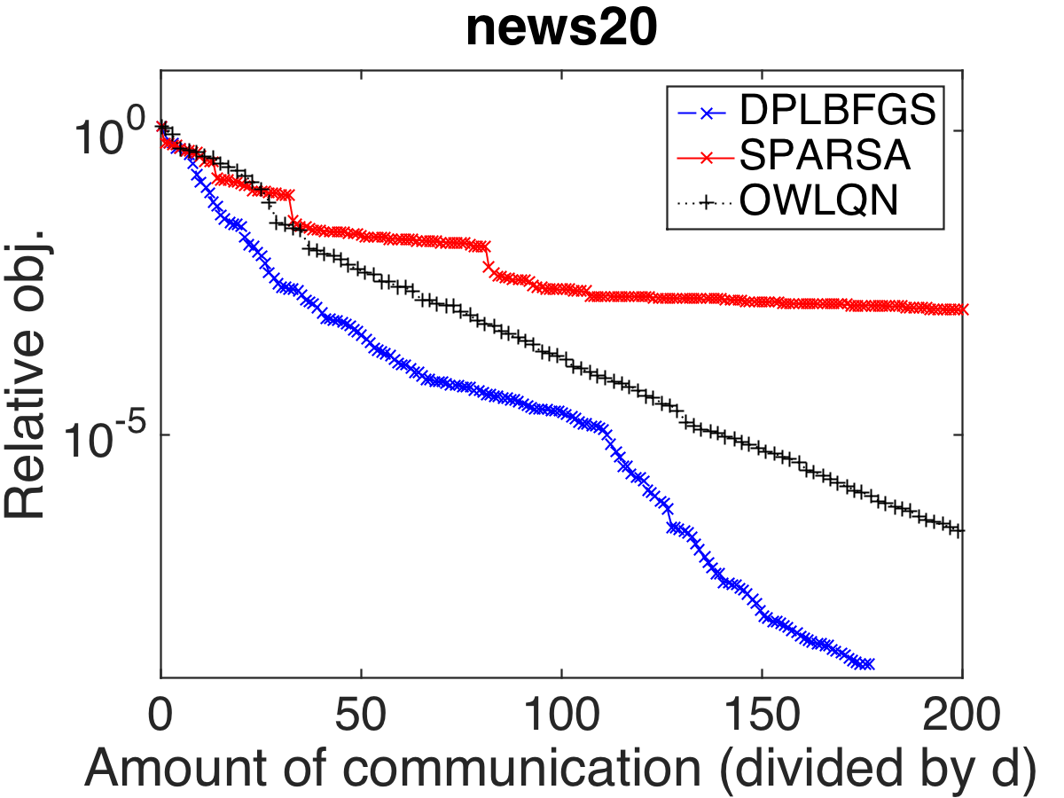
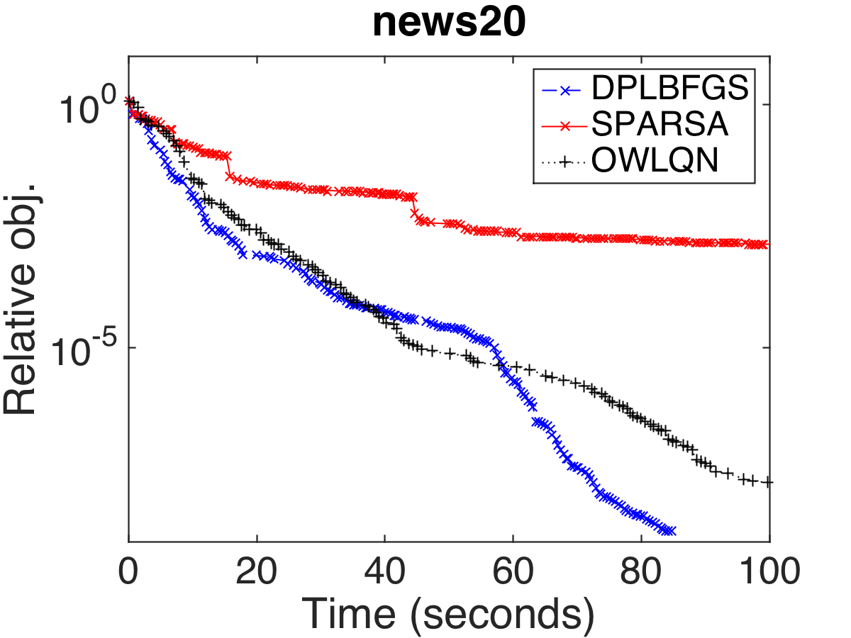
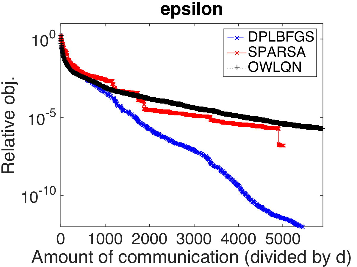
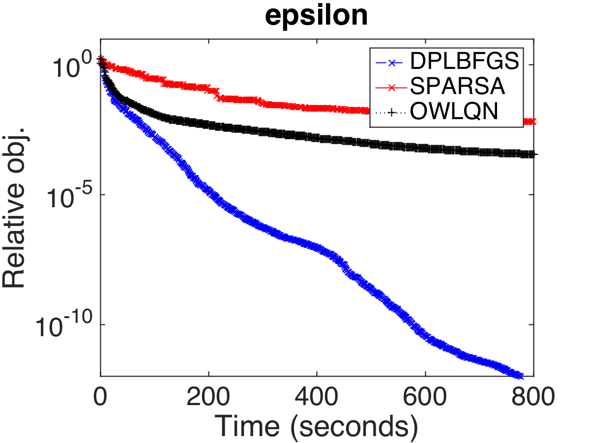
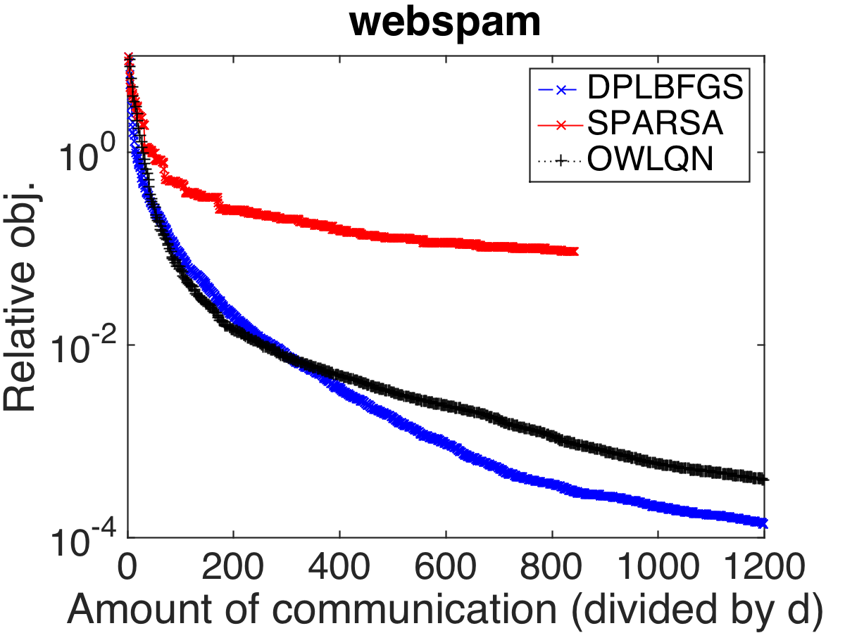
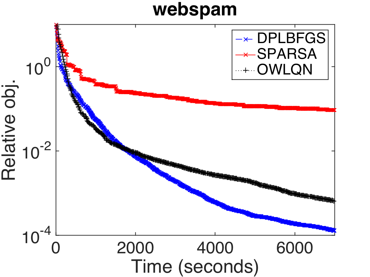
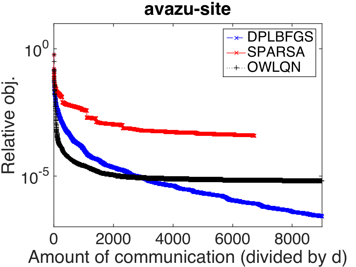
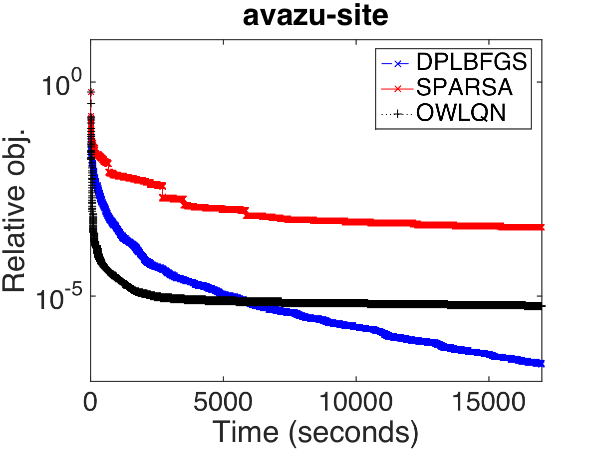
Figure 1: Comparison between different methods for (41) in terms of relative objective difference to the optimum. Left: communication (divided by $d$); right: running time (in seconds).

6.3 Comparison on the Dual Problem

Communication	Time

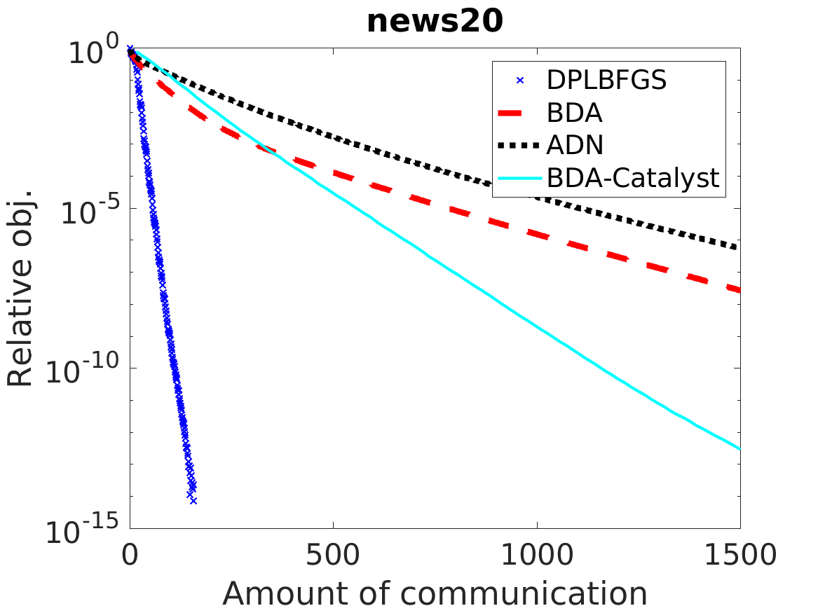
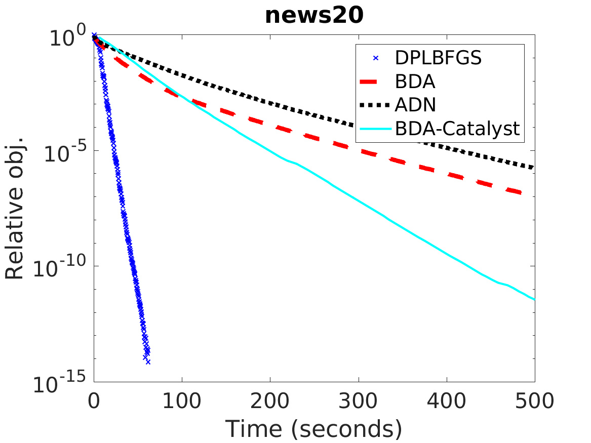
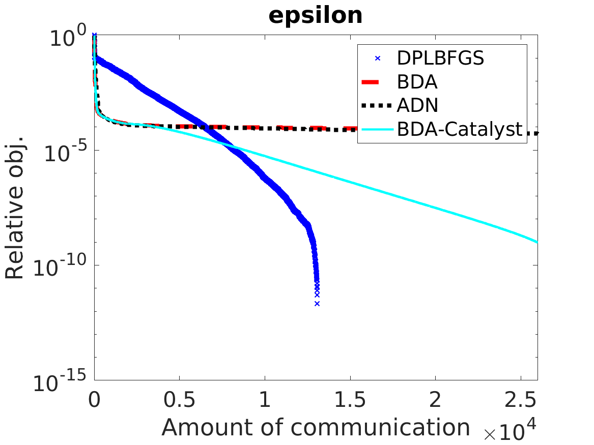
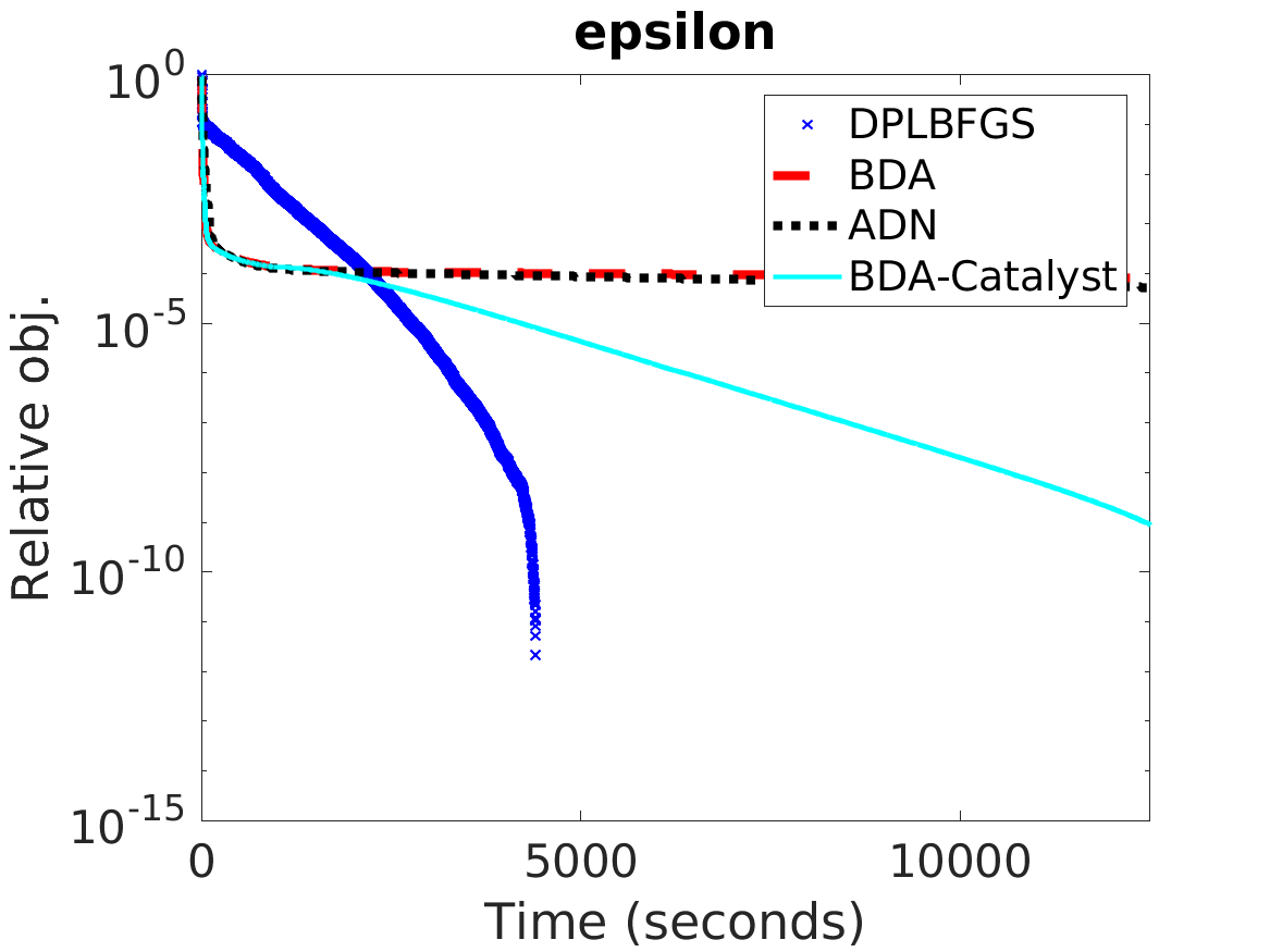
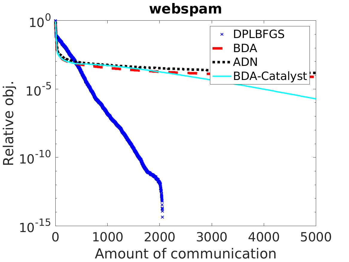
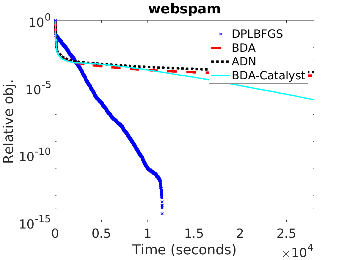
Figure 2: Comparison between different methods for (42) in terms of relative objective difference to the optimum. Left: communication (divided by $d$); right: running time (in seconds).

Communication	Time

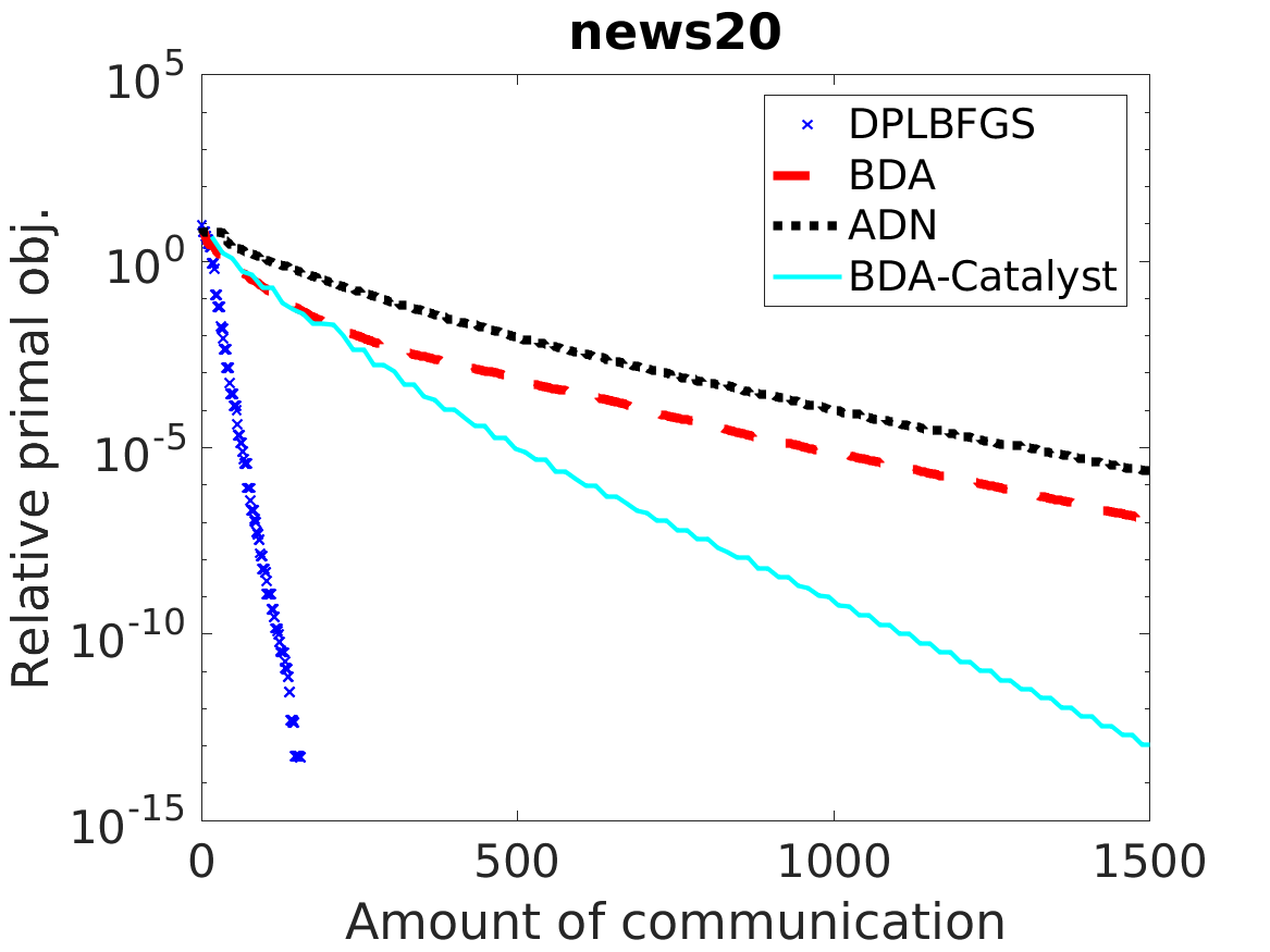
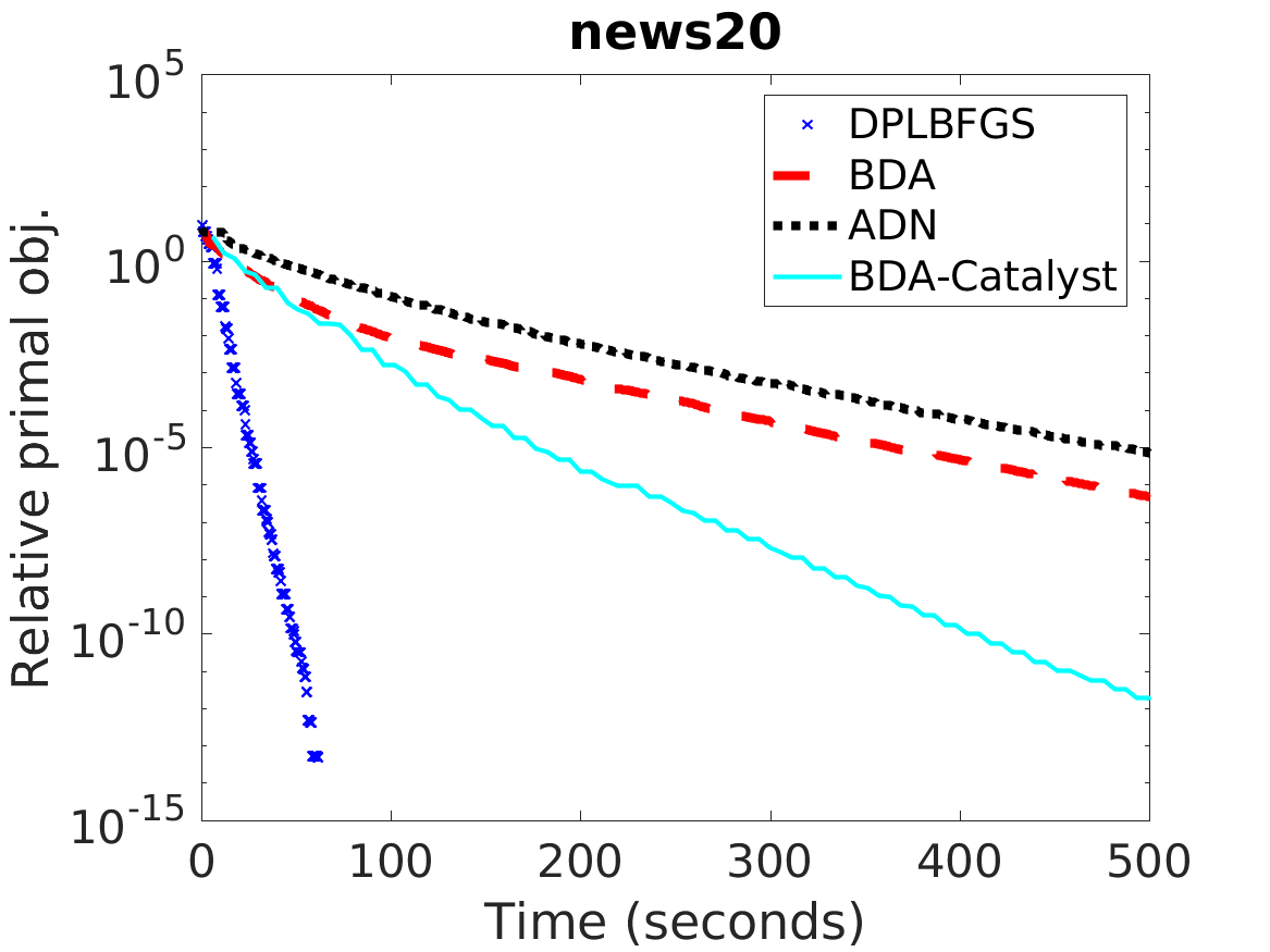
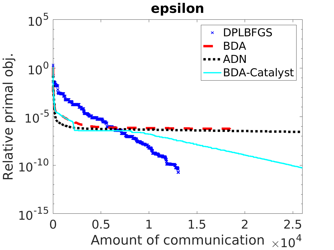
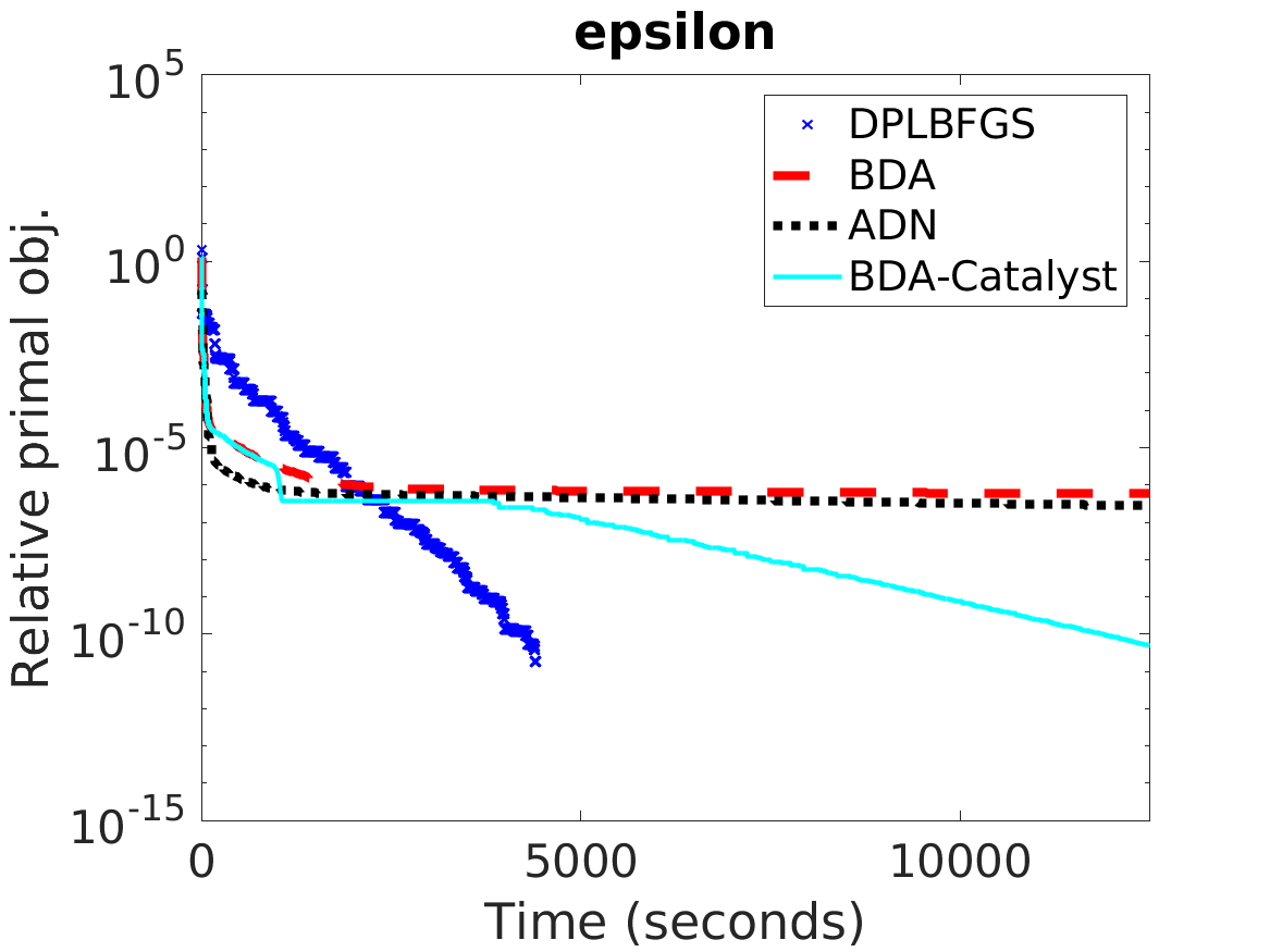
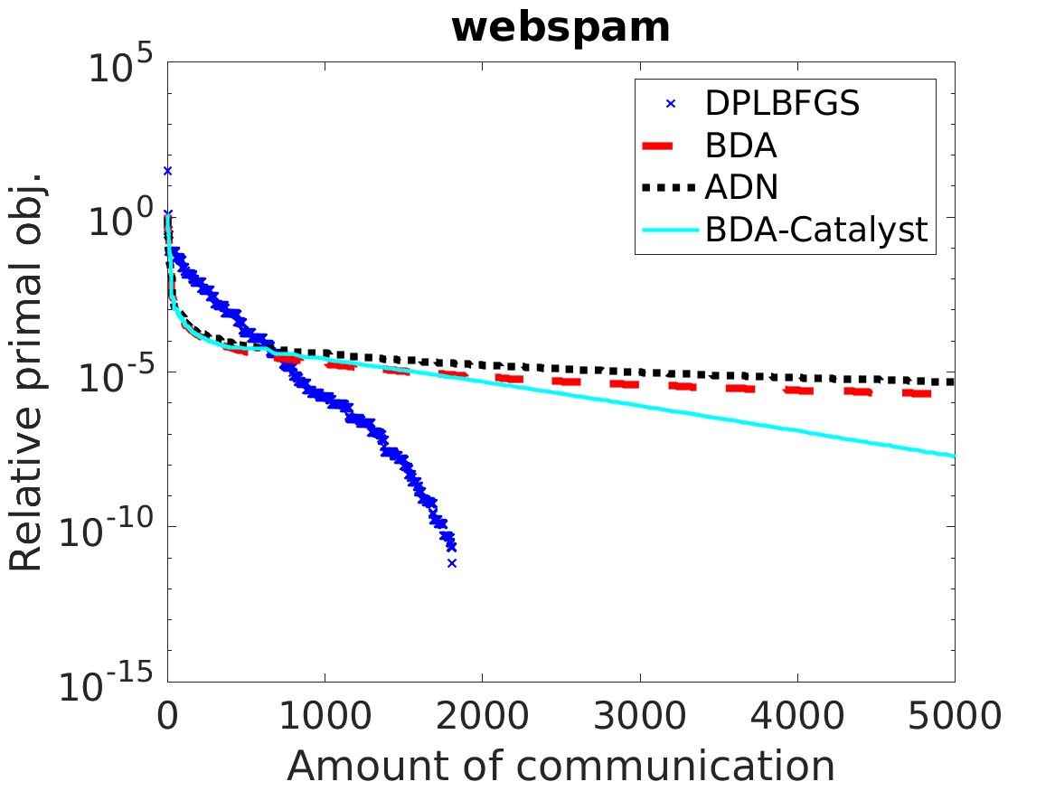
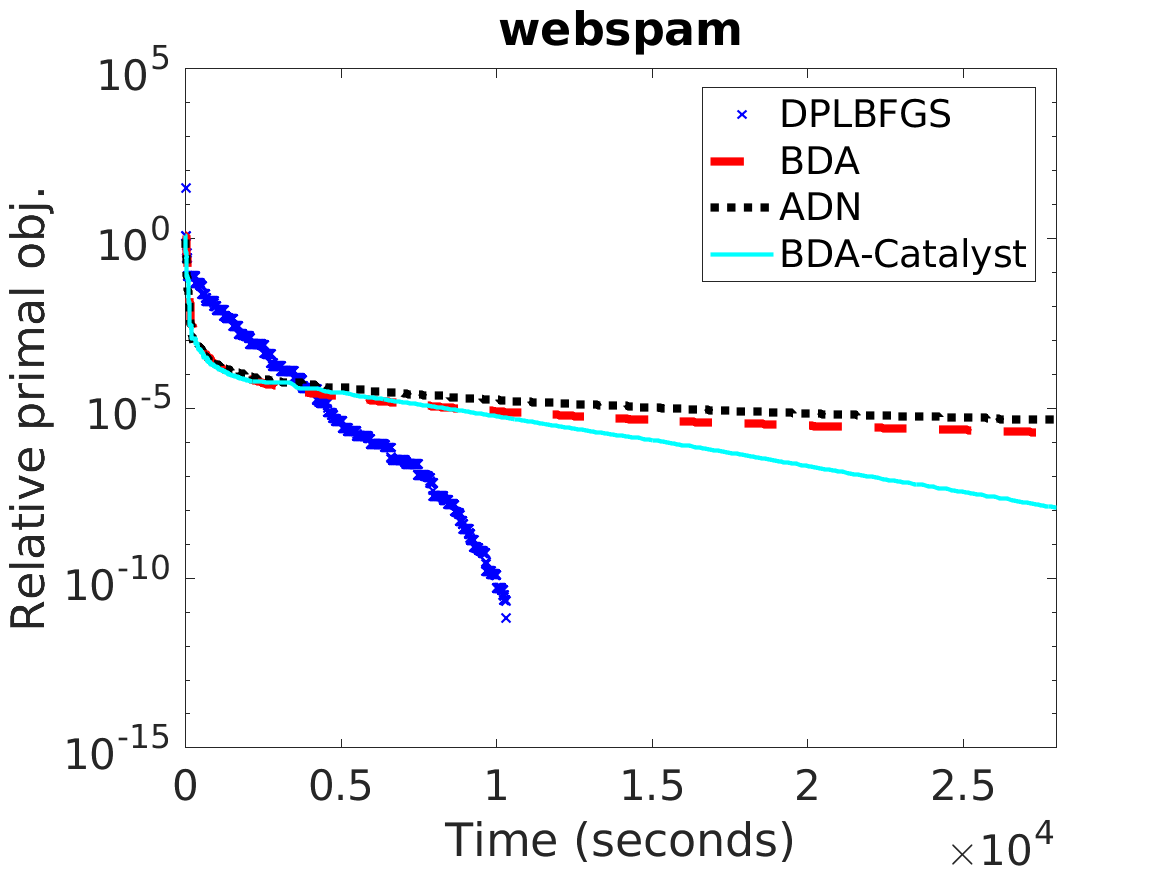
Figure 3: Comparison between different methods for (42) in terms of relative primal objective difference to the optimum. Left: communication (divided by $d$); right: running time (in seconds).

Now we turn to solve the dual problem, considering the specific example (42). We compare the following algorithms.

• BDA (Lee and Chang, 2019): a distributed algorithm using Block-Diagonal Approximation of the real Hessian of the smooth part with line search.

• BDA with Catalyst: using the BDA algorithm within the Catalyst framework (Lin et al., 2018) for accelerating first-order methods.

• ADN (Dünner et al., 2018): a trust-region approach where the quadratic term is a multiple of the block-diagonal part of the Hessian, scaled adaptively as the algorithm progresses.

• DPLBFGS-LS: our Distributed Proximal LBFGS approach. We fix $\epsilon_{1}=10^{-2}$ and limit the number of SpaRSA iterations to $100$. For the first ten iterations when $m(t)<m$, we use BDA to generate the update steps instead.

For BDA, we use the C/C++ implementation in the package MPI-LIBLINEAR. We implement ADN by modifying the above implementation of BDA. In both BDA and ADN, following Lee and Chang (2019) we use random-permutation coordinate descent (RPCD) for the local subproblems, and for each outer iteration we perform one epoch of RPCD. For the line search step in both BDA and DPLBFGS-LS, since the objective (42) is quadratic, we can find the exact minimizer efficiently (in closed form). The convergence guarantees still holds for exact line search, so we use this here in place of the backtracking approach described earlier.

We also applied the Catalyst framework (Lin et al., 2018) for accelerating first-order methods to BDA to tackle the dual problem, especially for dealing with the stagnant convergence issue. This framework requires a good estimate of the convergence rate and the strong convexity parameter $\sigma$. From (42), we know that $\sigma=1/(2C)$, but the actual convergence rate is hard to estimate as BDA interpolates between (stochastic) proximal coordinate descent (when only one machine is used) and proximal gradient (when $n$ machines are used). After experimenting with different sets of parameters for BDA with Catalyst, we found the following to work most effectively: for every outer iteration of the Catalyst framework, $K$ iterations of BDA is conducted with early termination if a negative step size is obtained from exact line search; for the next Catalyst iteration, the warm-start initial point is simply the iterate at the end of the previous Catalyst iteration; before starting Catalyst, we run the unaccelerated version of BDA for certain iterations to utilize its advantage of fast early convergence. Unfortunately, we do not find a good way to estimate the $\kappa$ term in the Catalyst framework that works for all data sets. Therefore, we find the best $\kappa$ by a grid search. We provide a detailed description of our implementation of the Catalyst framework on this problem and the related parameters used in this experiment in Appendix B.

We focus on the combination of Catalyst and BDA (instead of with ADN) for a few reasons. Since both BDA and ADN are distributed methods that use the block-diagonal portion of the Hessian matrix, it should suffice to evaluate the application of Catalyst to the better performing of the two to represent this class of algorithms. In addition, dealing with the trust-region adjustment of ADN becomes complicated as the problem changes through the Catalyst iterations.

The results are shown in Figure 2. We do not present results on the avazu data set in this experiment as all methods take extremely long time to converge. We first observe that, contrary to what is claimed in Dünner et al. (2018), BDA outperforms ADN on news20 and webspam, though the difference is insignificant, and the two are competitive on epsilon. This also justifies that applying the Catalyst framework on BDA alone suffices. Comparing our DPLBFGS approach to the block-diagonal ones, it is clear that our method performs magnitudes better than the state of the art in terms of both communication cost and time. For webspam and epsilon, the block-diagonal approaches are faster at first, but the progress stalls after a certain accuracy level. In contrast, while the proposed DPLBFGS approach does not converge as rapidly initially, the algorithm consistently makes progress towards a high accuracy solution.

As the purpose of solving the dual problem is to obtain an approximate solution to the primal problem through the formulation (40), we are interested on how the methods compare in terms of the primal solution precision. This comparison is presented in Figure 3. Since these dual methods are not descent methods for the primal problem, we apply the pocket approach (Gallant, 1990) suggested in Lee and Chang (2019) to use the iterate with the smallest primal objective so far as the current primal solution. We see that the primal objective values have trends very similar to the dual counterparts, showing that our DPLBFGS method is also superior at generating better primal solutions.

A potentially more effective approach is a hybrid one that first uses a block-diagonal method and then switches over to our DPLBFGS approach after the block-diagonal method hits the slow convergence phase. Developing such an algorithm would require a way to determine when we reach such a stage, and we leave the development of this method to future work. Another possibility is to consider a structured quasi-Newton approach to construct a Hessian approximation only for the off-block-diagonal part so that the block-diagonal part can be utilized simultaneously.

We also remark that our algorithm is partition-invariant in terms of convergence and communication cost, while the convergence behavior of the block-diagonal approaches depend heavily on the partition. This means when more machines are used, these block-diagonal approaches suffer from poorer convergence, while our method retains the same efficiency regardless of the number of machines begin used and how the data points are distributed (except for the initialization part).

7 Conclusions

In this work, we propose a practical and communication-efficient distributed algorithm for solving general regularized nonsmooth ERM problems. The proposed approach is the first one that can be applied both to the primal and the dual ERM problem under the instance-wise split scheme. Our algorithm enjoys fast performance both theoretically and empirically and can be applied to a wide range of ERM problems. Future work for the primal problem include active set identification for reducing the size of the vector communicated when the solution exhibits sparsity, and application to nonconvex applications; while for the dual problem, it is interesting to further exploit the structure so that the quasi-Newton approach can be combined with real Hessian entries at the block-diagonal part to get better convergence.

A Proofs

In this appendix, we provide proof for Lemma 1. The rest of Section 3 directly follows the results in Lee and Wright (2019b); Peng et al. (2018), and are therefore omitted. Note that (36) implies (34), and (34) implies (33) because $R_{0}^{2}$ is upper-bounded by $2(F(x^{0})-F^{*})/\mu$. Therefore, we get improved communication complexity by the fast early linear convergence from the general convex case.

Proof [Lemma 1] We prove the three results separately.

1. We assume without loss of simplicity that (17) is satisfied by all iterations. When it is not the case, we just need to shift the indices but the proof remains the same as the pairs of $({\boldsymbol{s}}_{t},{\boldsymbol{y}}_{t})$ that do not satisfy (17) are discarded.

   We first bound $\gamma_{t}$ defined in (15). From Lipschitz continuity of $\nabla f$, we have that for all $t$,

   $$\frac{\|{\boldsymbol{y}}_{t}\|^{2}}{{\boldsymbol{y}}_{t}^{\top}{\boldsymbol{s}}_{t}}\leq\frac{L^{2}\|{\boldsymbol{s}}_{t}\|^{2}}{{\boldsymbol{y}}_{t}^{\top}{\boldsymbol{s}}_{t}}\leq\frac{L^{2}}{\delta},$$ (43)

   establishing the upper bound. For the lower bound, (17) implies that

   $$\|{\boldsymbol{y}}_{t}\|\geq\delta\|{\boldsymbol{s}}_{t}\|,\quad\forall t.$$ (44)

   Therefore,

   $$\frac{{\boldsymbol{y}}_{t}^{\top}{\boldsymbol{s}}_{t}}{{\boldsymbol{y}}_{t}^{\top}{\boldsymbol{y}}_{t}}\leq\frac{\|{\boldsymbol{s}}_{t}\|}{\|{\boldsymbol{y}}_{t}\|}\leq\frac{1}{\delta},\quad\forall t.$$

   Following Liu and Nocedal (1989), $H_{t}$ can be obtained equivalently by

   $$H_{t}^{(0)} =\gamma_{t}I,$$

   $$H_{t}^{(k+1)} =H_{t}^{(k)}-\frac{H_{t}^{(k)}{\boldsymbol{s}}_{t-m(t)+k}{\boldsymbol{s}}_{t-m(t)+k}^{\top}H_{t}^{(k)}}{{\boldsymbol{s}}_{t-m(t)+k}^{\top}H_{t}^{(k)}{\boldsymbol{s}}_{t-m(t)+k}}+\frac{{\boldsymbol{y}}_{t-m(t)+k}{\boldsymbol{y}}_{t-m(t)+k}^{\top}}{{\boldsymbol{y}}_{t-m(t)+k}^{\top}{\boldsymbol{s}}_{t-m(t)+k}},\;\;k=0,\dots,m(t)-1,$$ (45)

   $$H_{t} =H_{t}^{(m(t))}.$$

   Therefore, we can bound the trace of $H_{t}^{(}k)$ and hence $H_{t}$ through (43).

   $$\mbox{\rm trace}\left(H_{t}^{(k)}\right)\leq\mbox{\rm trace}\left(H_{t}^{(0)}\right)+\sum_{j=t-m(t)}^{t-m(t)+k}\frac{{\boldsymbol{y}}_{j}^{\top}{\boldsymbol{y}}_{j}}{{\boldsymbol{y}}_{j}^{\top}{\boldsymbol{s}}_{j}}\leq\gamma_{t}N+\frac{kL^{2}}{\delta},\quad\forall t,$$ (46)

   where $N$ is the matrix dimension. According to Byrd et al. (1994), the matrix $H^{(k)}_{t}$ is equivalent to the inverse of

   $$B^{(k)}_{t} \coloneqq V^{\top}_{t-m(t)+k}\cdots V^{\top}_{t-m(t))}B_{t}^{0}V_{t-m(t)}\cdots V_{t-m(t)+k}+\rho_{t-m(t)+k}{\boldsymbol{s}}_{t-m(t)+k}{\boldsymbol{s}}_{t-m(t)+k}^{\top}+$$

   $$\qquad\sum_{j=t-m(t)}^{t-m(t)-1+k}\rho_{j}V_{t-m(t)+k}^{\top}\cdots V_{j+1}^{\top}{\boldsymbol{s}}_{j}{\boldsymbol{s}}_{j}^{\top}V_{j+1}\cdots V_{t-m(t)+k},$$ (47)

   where for $j\geq 0$,

   $$V_{j}\coloneqq I-\rho_{j}{\boldsymbol{y}}_{j}{\boldsymbol{s}}_{j}^{\top},\quad\rho_{j}\coloneqq\frac{1}{{\boldsymbol{y}}_{j}^{\top}{\boldsymbol{s}}_{j}},\quad B_{t}^{0}=\frac{1}{\gamma_{t}}I.$$

   From the form (47), it is clear that $B_{t}^{(k)}$ and hence $H_{t}$ are all positive-semidefinite because $\gamma_{t}\geq 0,\rho_{j}>0$ for all $j$ and $t$. Therefore, from positive semidefiniteness, (46) implies the existence of $c_{1}>0$ such that

   $$H_{t}^{(k)}\preceq c_{1}I,\quad k=0,\dotsc,m(t),\quad\forall t.$$

   Next, for its lower bound, from the formulation for (45) in Liu and Nocedal (1989), and the upper bound $\|H_{t}^{(k)}\|\leq c_{1}$, we have

   $$\det\left(H_{t}\right)=\det\left(H_{t}^{(0)}\right)\prod_{k=t-m(t)}^{t-1}\frac{{\boldsymbol{y}}_{k}^{\top}{\boldsymbol{s}}_{k}}{{\boldsymbol{s}}_{k}^{\top}{\boldsymbol{s}}_{k}}\frac{{\boldsymbol{s}}_{k}^{\top}{\boldsymbol{s}}_{k}}{{\boldsymbol{s}}_{k}^{\top}H_{t}^{(k-t+m(t))}{\boldsymbol{s}}_{k}}\geq\gamma_{t}^{N}\left(\frac{\delta}{c_{1}}\right)^{m(t)}\geq M_{1}.$$

   for some $M_{1}>0$. From that the eigenvalues of $H_{t}$ are upper-bounded and nonnegative, and from the lower bound of the determinant, the eigenvalues of $H_{t}$ are also lower-bounded by a positive value $c_{2}$, completing the proof.

2. By directly expanding $\nabla\hat{f}$, we have that for any $p_{1},p_{2}$,

   $$\nabla\hat{f}(p_{1})-\nabla\hat{f}(p_{2})=\nabla f(x)+Hp_{1}-\left(\nabla f(x)+Hp_{2}\right)=H(p_{1}-p_{2}).$$

   Therefore, we have

   $$\frac{\left(\nabla\hat{f}(p_{1})-\nabla\hat{f}(p_{2})\right)^{\top}\left(p_{1}-p_{2}\right)}{\left\|p_{1}-p_{2}\right\|^{2}}=\frac{\left\|p_{1}-p_{2}\right\|_{H}^{2}}{\left\|p_{1}-p_{2}\right\|^{2}}\in\left[c_{2},c_{1}\right]$$

   for bounding $\psi_{i}$ for $i>0$, and the bound for $\psi_{0}$ is directly from the bounds of $\gamma_{t}$. The combined bound is therefore $[\min\{c_{2},\delta\},\max\{c_{1},L^{2}/\delta\}]$. Next, we show that the final $\psi_{i}$ is always upper-bounded. The right-hand side of (20) is equivalent to the following:

   $$\arg\min_{\boldsymbol{d}}\,\hat{Q}_{\psi_{i}}\left({\boldsymbol{d}}\right)\coloneqq\nabla\hat{f}\left(p^{(i)}\right)^{\top}{\boldsymbol{d}}+\frac{\psi_{i}\left\|{\boldsymbol{d}}\right\|^{2}}{2}+\hat{\Psi}\left({\boldsymbol{d}}+p\right)-\hat{\Psi}\left(p\right).$$ (48)

   Denote the solution by ${\boldsymbol{d}}$, then we have $p^{(i+1)}=p^{(i)}+{\boldsymbol{d}}$. Note that we allow ${\boldsymbol{d}}$ to be an approximate solution. Because $H$ is upper-bounded by $c_{1}$, we have that $\nabla\hat{f}$ is $c_{1}$-Lipschitz continuous. Therefore,

   $$Q\left(p^{(i+1)}\right)-Q\left(p^{(i)}\right)\leq ~{}\nabla\hat{f}(p^{(i)})^{\top}\left(p^{(i+1)}-p^{(i)}\right)+\frac{c_{1}}{2}\left\|p^{(i+1)}-p^{(i)}\right\|^{2}+\hat{\Psi}\left(p^{(i+1)}\right)-\hat{\Psi}\left(p^{(i)}\right)$$

   $$\stackrel{{\scriptstyle\eqref{eq:hatQ}}}{{=}} ~{}\hat{Q}_{\psi_{i}}({\boldsymbol{d}})-\frac{\psi_{i}}{2}\left\|{\boldsymbol{d}}\right\|^{2}+\frac{c_{1}}{2}\left\|{\boldsymbol{d}}\right\|^{2}.$$ (49)

   As $\hat{Q}_{\psi_{i}}(0)=0$, provided that the approximate solution ${\boldsymbol{d}}$ is better than the point $0$, we have

   $$\hat{Q}({\boldsymbol{d}})\leq\hat{Q}(0)=0.$$ (50)

   Putting (50) into (49), we obtain

   $$Q\left(p^{(i+1)}\right)-Q\left(p^{(i)}\right)\leq\frac{c_{1}-\psi_{i}}{2}\|{\boldsymbol{d}}\|^{2}.$$

   Therefore, whenever

   $$\frac{c_{1}-\psi_{i}}{2}\leq-\frac{\sigma_{0}\psi_{i}}{2},$$

   (22) holds. This is equivalent to

   $$\psi_{i}\geq\frac{c_{1}}{1-\sigma_{0}},$$

   Note that the initialization of $\psi_{i}$ is upper-bounded by $c_{1}$ for all $i>1$, so the final $\psi_{i}$ is indeed upper-bounded. Together with the first iteration where we start with $\psi_{0}=\gamma_{t}$, we have that $\psi_{i}$ for all $i$ are always bounded from the boundedness of $\gamma_{t}$.

3. From the results above, at every iteration, SpaRSA finds the update direction by constructing and optimizing a quadratic approximation of $\hat{f}(x)$, where the quadratic term is a multiple of identity, and its coefficient is bounded in a positive range. Therefore, the theory developed by Lee and Wright (2019b) can be directly used to show the desired result even if (20) is solved only approximately. For completeness, we provide a simple proof for the case that (20) is solved exactly.

   We note that since $Q$ is $c_{2}$-strongly convex, the following condition holds.

   $$\frac{\min_{{\boldsymbol{s}}\in\nabla\hat{f}\left(p^{(i+1)}\right)+\partial\hat{g}\left(p^{(i+1)}\right)}\left\|{\boldsymbol{s}}\right\|^{2}}{2c_{2}}\geq Q\left(p^{(i+1)}\right)-Q^{*}.$$ (51)

   On the other hand, from the optimality condition of (48), we have that for the optimal solution ${\boldsymbol{d}}^{*}$ of (48),

   $$-\psi_{i}{\boldsymbol{d}}^{*}=\nabla\hat{f}\left(p^{(i)}\right)+{\boldsymbol{s}}_{i+1},$$ (52)

   for some

   $${\boldsymbol{s}}_{i+1}\in\partial\hat{\Psi}\left(p^{(i+1)}\right).$$

   Therefore,

   $$Q\left(p^{(i+1)}\right)-Q^{*}\stackrel{{\scriptstyle\eqref{eq:kl}}}{{\leq}} ~{}\frac{1}{2c_{2}}\left\|\nabla\hat{f}\left(p^{(i+1)}\right)-\nabla\hat{f}\left(p^{(i)}\right)+\nabla\hat{f}\left(p^{(i)}\right)+{\boldsymbol{s}}_{i+1}\right\|^{2}$$

   $$\stackrel{{\scriptstyle\eqref{eq:dopt}}}{{\leq}} ~{}\frac{1}{c_{2}}\left\|\nabla\hat{f}\left(p^{(i+1)}\right)-\nabla\hat{f}\left(p^{(i)}\right)\right\|^{2}+\left\|\psi_{i}{\boldsymbol{d}}^{*}\right\|^{2}$$

   $$\leq ~{}\frac{1}{c_{2}}\left(c_{1}^{2}+\psi_{i}^{2}\right)\left\|{\boldsymbol{d}}^{*}\right\|^{2}.$$ (53)

   By combining (22) and (53), we obtain

   $$Q\left(p^{(i+1)}\right)-Q\left(p^{(i)}\right)\leq-\frac{\sigma_{0}\psi_{i}}{2}\left\|{\boldsymbol{d}}^{*}\right\|^{2}\leq-\frac{\sigma_{0}\psi_{i}}{2}\frac{c_{2}}{c_{1}^{2}+\psi_{i}^{2}}\left(Q\left(p^{(i+1)}\right)-Q^{*}\right).$$

   Rearranging the terms, we obtain

   $$\left(1+\frac{c_{2}\sigma_{0}\psi_{i}}{2(c_{1}^{2}+\psi^{2})}\right)\left(Q\left(p^{(i+1)}\right)-Q^{*}\right)\leq Q\left(p^{(i)}\right)-Q^{*},$$

   showing Q-linear convergence of SpaRSA, with

   $$\eta=\sup_{i=0,1,\dotsc}\quad\left(1+\frac{c_{2}\sigma_{0}\psi_{i}}{2\left(c_{1}^{2}+\psi_{i}^{2}\right)}\right)^{-1}\in[0,1).$$

   Note that since $\psi_{i}$ are bounded in a positive range, we can find this supremum in the desired range.

 

B Implementation Details and Parameter Selection for the Catalyst Framework

We first give an overview to the version of Catalyst framework for strongly-convex problems (Lin et al., 2018) for accelerating convergence rate of first-order methods, then describe our implementation details in the experiment in Section 6.3. The Catalyst framework is described in Algorithm 3.

1:  Input: $x^{0}\in\mathbb{R}^{N}$, a smoothing parameter $\kappa$, the strong convexity parameter $\mu$, an optimization method $\mathcal{M}$, and a stopping criterion for the inner optimization.

2:  Initialize $y^{0}=x^{0}$, $q=\mu/(\mu+\kappa)$, $\beta=(1-\sqrt{q})/(1+\sqrt{q})$.

3:  for $k=1,2,\dotsc,$ do

4:     Use $\mathcal{M}$ with the input stopping condition to approximately optimize

$$\min_{x}\quad F(x)+\frac{\kappa}{2}\|x-y^{k-1}\|^{2}$$ (54)

from a warm-start point $x^{k}_{0}$ to obtain the iterate $x^{k}$.

5:     $y_{k}=x^{k}+\beta(x^{k}-x^{k-1})$.

6:  end for

7:  Output $x^{k}$.

Algorithm 3 Catalyst Framework for optimizing strongly-convex (11).

According to Lin et al. (2018), when $\mathcal{M}$ is the proximal gradient method, the ideal value of $\kappa$ is $\max(L-2\mu,0)$, and when $L>2\mu$, the convergence speed can be improved to the same order as accelerated proximal gradient (up to a logarithm factor difference). Similarly, when $\mathcal{M}$ is stochastic proximal coordinate descent with uniform sampling, by taking $\kappa=\max(L_{\max}-2\mu,0)$, where $L_{\max}$ is the largest block Lipschitz constant, one can obtain convergence rate similar to that of accelerated coordinate descent. Since when using proximal coordinate descent as the local solver, both BDA and ADN interpolate between proximal coordinate descent and proximal gradient, depending on the number of machines, it is intuitive that acceleration should work for them.

Considering (42), the problem is clearly strongly convex with parameter $1/(2C)$, thus we take $\mu=1/(2C)$. For the stopping condition, we use the simple fixed iteration choice suggested in Lin et al. (2018) (called (C3) in their notation). Empirically we found a very effective way is to run $K$ iterations of BDA with early termination whenever a negative step size is obtained from exact line search. For the warm-start part, although (42) is a regularized problem, the objective part is smooth, so we take their suggestion for smooth problem to use $x^{k}_{0}=x^{k-1}$. Note that they suggested that for general regularized problems, one should take one proximal gradient step of the original $F$ at $x^{k-1}$ to obtain $x^{k}_{0}$. We also experimented with this choice, but preliminary results show that using $x^{k-1}$ gives better initial objective value for (54).

The next problem is how to select $\kappa$. We observe that for webspam and epsilon, the convergence of both BDA and ADN clearly falls into two stages. Through some checks, we found that the first stage can barely be improved. On the other hand, if we pick a value of $\kappa$ that can accelerate convergence at the later stage, the fast early convergence behavior is not present anymore, thus it takes a long time for the accelerated approach to outperform the unaccelerated version. To get better results, we take an approach from the hindsight: first start with the unaccelerated version with a suitable number of iterations, and then we switch to Catalyst with $\kappa$ properly chosen by grid search for accelerating convergence at the later stage. The parameters in this approach is recorded in Table 4. We note that this way of tuning from the hindsight favors the accelerated method unfairly, as it takes information obtained through running other methods first. In particular, it requires the optimal objective (obtained by first solving the problem through other methods) and running the unaccelerated method to know the turning point of the convergence stages (requires the optimal objective to compute). Parameter tuning for $\kappa$ is also needed. These additional efforts are not included in the running time comparison, so our experimental result does not suggest that the accelerated method is better than the unaccelerated version. The main purpose is to show that our proposed approach also outperforms acceleration methods with careful parameter choices.

Table 4: Catalyst parameters.

Data set	#BDA iterations before starting Catalyst	$\kappa$
news	$0$	$17$
epsilon	$2,000$	$12,000$
webspam	$400$	$2,000$

References

- Anderson et al. (1999) Edward Anderson, Zhaojun Bai, Christian Bischof, L Susan Blackford, James Demmel, Jack Dongarra, Jeremy Du Croz, Anne Greenbaum, Sven Hammarling, Alan McKenney, et al. LAPACK Users’ guide. SIAM, 1999.
- Andrew and Gao (2007) Galen Andrew and Jianfeng Gao. Scalable training of L1-regularized log-linear models. In Proceedings of the International Conference on Machine Learning, pages 33–40, 2007.
- Bach (2015) Francis Bach. Duality between subgradient and conditional gradient methods. SIAM Journal on Optimization, 25(1):115–129, 2015.
- Beck and Teboulle (2009) Amir Beck and Marc Teboulle. A fast iterative shrinkage-thresholding algorithm for linear inverse problems. SIAM Journal on Imaging Sciences, 2(1):183–202, 2009.
- Bonettini et al. (2016) Silvia Bonettini, Ignace Loris, Federica Porta, and Marco Prato. Variable metric inexact line-search-based methods for nonsmooth optimization. SIAM Journal on Optimization, 26(2):891–921, 2016.
- Boyd and Vandenberghe (2004) Stephen Boyd and Lieven Vandenberghe. Convex Optimization. Cambridge University Press, 2004.
- Byrd et al. (1994) Richard H. Byrd, Jorge Nocedal, and Robert B. Schnabel. Representations of quasi-Newton matrices and their use in limited memory methods. Mathematical Programming, 63(1-3):129–156, 1994.
- Chan et al. (2007) Ernie Chan, Marcel Heimlich, Avi Purkayastha, and Robert Van De Geijn. Collective communication: theory, practice, and experience. Concurrency and Computation: Practice and Experience, 19(13):1749–1783, 2007.
- Dünner et al. (2018) Celestine Dünner, Aurelien Lucchi, Matilde Gargiani, An Bian, Thomas Hofmann, and Martin Jaggi. A distributed second-order algorithm you can trust. In Proceedings of the International Conference on Machine Learning, 2018.
- Gallant (1990) Stephen I. Gallant. Perceptron-based learning algorithms. Neural Networks, IEEE Transactions on, 1(2):179–191, 1990.
- Ghanbari and Scheinberg (2018) Hiva Ghanbari and Katya Scheinberg. Proximal quasi-Newton methods for regularized convex optimization with linear and accelerated sublinear convergence rates. Computational Optimization and Applications, 69(3):597–627, 2018.
- Hiriart-Urruty and Lemaréchal (2001) Jean-Baptiste Hiriart-Urruty and Claude Lemaréchal. Fundamentals of convex analysis. Springer Science & Business Media, 2001.
- Lee and Chang (2019) Ching-pei Lee and Kai-Wei Chang. Distributed block-diagonal approximation methods for regularized empirical risk minimization. Machine Learning, 2019. To appear.
- Lee and Wright (2017) Ching-pei Lee and Stephen J. Wright. Using neural networks to detect line outages from PMU data. Technical report, 2017.
- Lee and Wright (2019a) Ching-pei Lee and Stephen J. Wright. Random permutations fix a worst case for cyclic coordinate descent. IMA Journal of Numerical Analysis, 39(3):1246–1275, 2019a.
- Lee and Wright (2019b) Ching-pei Lee and Stephen J. Wright. Inexact successive quadratic approximation for regularized optimization. Computational Optimization and Applications, 72:641–674, 2019b.
- Lee et al. (2017) Ching-pei Lee, Po-Wei Wang, Weizhu Chen, and Chih-Jen Lin. Limited-memory common-directions method for distributed optimization and its application on empirical risk minimization. In Proceedings of the SIAM International Conference on Data Mining, 2017.
- Lee et al. (2018) Ching-pei Lee, Cong Han Lim, and Stephen J. Wright. A distributed quasi-Newton algorithm for empirical risk minimization with nonsmooth regularization. In Proceedings of the 24th ACM SIGKDD International Conference on Knowledge Discovery & Data Mining, pages 1646–1655, New York, NY, USA, 2018. ACM.
- Lee et al. (2014) Jason D. Lee, Yuekai Sun, and Michael A. Saunders. Proximal Newton-type methods for minimizing composite functions. SIAM Journal on Optimization, 24(3):1420–1443, 2014.
- Li and Fukushima (2001) Dong-Hui Li and Masao Fukushima. On the global convergence of the BFGS method for nonconvex unconstrained optimization problems. SIAM Journal on Optimization, 11(4):1054–1064, 2001.
- Lin et al. (2014) Chieh-Yen Lin, Cheng-Hao Tsai, Ching-Pei Lee, and Chih-Jen Lin. Large-scale logistic regression and linear support vector machines using Spark. In Proceedings of the IEEE International Conference on Big Data, pages 519–528, 2014.
- Lin et al. (2018) Hongzhou Lin, Julien Mairal, and Zaid Harchaoui. Catalyst acceleration for first-order convex optimization: from theory to practice. Journal of Machine Learning Research, 18(212):1–54, 2018.
- Liu and Nocedal (1989) Dong C. Liu and Jorge Nocedal. On the limited memory BFGS method for large scale optimization. Mathematical programming, 45(1):503–528, 1989.
- Meng et al. (2016) Xiangrui Meng, Joseph Bradley, Burak Yavuz, Evan Sparks, Shivaram Venkataraman, Davies Liu, Jeremy Freeman, DB Tsai, Manish Amde, Sean Owen, et al. MLlib: Machine learning in Apache Spark. Journal of Machine Learning Research, 17(1):1235–1241, 2016.
- Message Passing Interface Forum (1994) Message Passing Interface Forum. MPI: a message-passing interface standard. International Journal on Supercomputer Applications, 8(3/4), 1994.
- Nesterov (1983) Yurii Nesterov. A method of solving a convex programming problem with convergence rate . Soviet Mathematics Doklady, 27:372–376, 1983.
- Nesterov (2013) Yurii Nesterov. Gradient methods for minimizing composite functions. Mathematical Programming, 140(1):125–161, 2013.
- Peng et al. (2018) Wei Peng, Hui Zhang, and Xiaoya Zhang. Global complexity analysis of inexact successive quadratic approximation methods for regularized optimization under mild assumptions. Technical report, 2018.