$Sp(4)$ gauge theories on the lattice: Quenched fundamental and antisymmetric fermions

Abstract

We perform lattice studies of meson mass spectra and decay constants of the $Sp(4)$ gauge theory in the quenched approximation. We consider two species of (Dirac) fermions as matter field content, transforming in the 2-index antisymmetric and the fundamental representation of the gauge group, respectively. All matter fields are formulated as Wilson fermions. We extrapolate to the continuum and massless limits, and compare to each other the results obtained for the two species of mesons. In the case of two fundamental and three antisymmetric fermions, the long-distance dynamics is relevant for composite Higgs models. This is the first lattice study of this class of theories. The global $SU(4)\times SU(6)$ symmetry is broken to the $Sp(4)\times SO(6)$ subgroup, and the condensates align with the explicit mass terms present in the lattice formulation of the theory.

The main results of our quenched calculations are that, with fermions in the 2-index antisymmetric representation of the group, the masses squared and decay constant squared of all the mesons we considered are larger than the corresponding quantities for the fundamental representation, by factors that vary between $\sim 1.2$ and $\sim 2.7$. We also present technical results that will be useful for future lattice investigations of dynamical simulations, of composite chimera baryons, and of the approach to large $N$ in the $Sp(2N)$ theories considered. We briefly discuss their high-temperature behaviour, where symmetry restoration and enhancement are expected.

I Introduction

In composite Higgs models (CHMs) Kaplan:1983fs ; Georgi:1984af ; Dugan:1984hq , the Higgs fields, responsible for electroweak symmetry breaking, arise as pseudo-Nambu-Goldstone bosons (pNGBs) in a more fundamental theory, hence addressing the little hierarchy problem of generic extensions of the Standard Model (SM) of particle physics. In comparison to the other SM fermions, the top quark has a large mass, making it heavier than the $W$, the $Z$, and even the recently discovered Higgs boson Aad:2012tfa ; Chatrchyan:2012xdj . It is then natural to complete the CHM scenario by postulating that also the top quark has composite nature, at least partially, at the fundamental level. The additional model-building dimension added to this framework by (partial) top compositeness yields a richness of potential implications that has been explored in the literature on the subject in a range of possible directions, and motivates us to study its dynamical origin with nonperturbative techniques. The literature on composite Higgs models is indeed vast (see for instance Refs. Agashe:2004rs ; Contino:2006qr ; Barbieri:2007bh ; Lodone:2008yy ; Marzocca:2012zn ; Grojean:2013qca ; Ferretti:2013kya ; Cacciapaglia:2014uja ; Arbey:2015exa ; Vecchi:2015fma ; Panico:2015jxa ; Ferretti:2016upr ; Agugliaro:2016clv ; Alanne:2017rrs ; Feruglio:2016zvt ; DeGrand:2016pgq ; Fichet:2016xvs ; Galloway:2016fuo ; Csaki:2017cep ; Chala:2017sjk ; Csaki:2017jby ; Ayyar:2017qdf ; Alanne:2017ymh ; Ayyar:2018zuk ; Ayyar:2018ppa ; Cai:2018tet ; Agugliaro:2018vsu ; Ayyar:2018glg ; Cacciapaglia:2018avr ; Witzel:2019jbe ; Cacciapaglia:2019bqz ; Ayyar:2019exp ; Cossu:2019hse ; Cacciapaglia:2019ixa ; BuarqueFranzosi:2019eee ), especially in connection with dynamical theories characterised by the $SU(4)/Sp(4)$ coset (see for instance Refs. Katz:2005au ; Gripaios:2009pe ; Barnard:2013zea ; Lewis:2011zb ; Hietanen:2014xca ; Arthur:2016dir ; Arthur:2016ozw ; Pica:2016zst ; Detmold:2014kba ; Lee:2017uvl ; Cacciapaglia:2015eqa ; Bizot:2016zyu ; Hong:2017smd ; Golterman:2017vdj ; Drach:2017btk ; Sannino:2017utc ; Alanne:2018wtp ; Bizot:2018tds ; BuarqueFranzosi:2018eaj ; Gertov:2019yqo ; Cacciapaglia:2019dsq ).

In Ref. Bennett:2017kga (see also Refs. Bennett:2017tum ; Bennett:2017ttu and the more recent Refs. Bennett:2017kbp ; Lee:2018ztv ; Bennett:2019jzz ; Bennett:2019ckt ), some of us proposed a systematic programme of exploration of the lattice dynamics of $Sp(2N)$ gauge theories. Our main scientific motivation is the application of the results of such studies to the CHM context. In order to realise also top compositeness, it is necessary to implement on the lattice matter fields with mixed representations. For example, the model discussed in Refs. Barnard:2013zea ; Ferretti:2013kya requires that the matter content consists of $N_{f}=2$ Dirac fields transforming in the fundamental representation of $Sp(2N)$, supplemented by $n_{f}=3$ Dirac fields transforming in the antisymmetric representation of $Sp(2N)$. This dynamical system is expected to yield the spontaneous breaking of the $SU(4)\times SU(6)$ global symmetry to its $Sp(4)\times SO(6)$ subgroup. The introduction of diagonal mass terms for the fermions is compatible (aligned) with the vacuum structure, and provides a degenerate nonvanishing mass for the resulting $5+20$ pNGBs. The lattice treatment of such a system with multiple dynamical fermion representations is a novel arena for lattice gauge theories, and only recently have calculations of this type been published, in the specific context of theories with $SU(4)$ gauge group DeGrand:2016pgq ; Ayyar:2017qdf ; Ayyar:2018zuk ; Ayyar:2018glg ; Cossu:2019hse .

In this paper, we take a first step in this direction for $Sp(2N)$ gauge theories. We consider the $Sp(4)$ gauge theory, and treat the two species of fermions in the quenched approximation; only the gluon dynamics is captured by the lattice numerical study, but the operators used to compute the relevant correlation functions involve both types of matter fields. We compute the mass spectra and decay constants of the mesons built both with fundamental and antisymmetric fermions, and perform their continuum extrapolation. We compare the properties of mesonic observables obtained with the two representations, which, in the dynamical theory, is important for CHM phenomenology. Since very little is known about the $Sp(2N)$ gauge theories, our quenched study is a first benchmark of these theories and would serve as a starting point for a more extensive and detailed investigation of such models.

We treat the relevant degrees of freedom with a low-energy effective field theory (EFT) that we employ to analyse the numerical data extrapolated to the continuum limit. The EFT proposed in Ref. Bennett:2017kga for the theory with $SU(4)/Sp(4)$ coset is based on the ideas of hidden local symmetry, adapted from Refs. Bando:1984ej ; Casalbuoni:1985kq ; Bando:1987br ; Casalbuoni:1988xm ; Harada:2003jx (and Georgi:1989xy ; Appelquist:1999dq ; Piai:2004yb ; Franzosi:2016aoo ), and supplemented by some simplifying working assumptions. Here we return to the EFT to improve it and to generalise it to the case of the $SU(6)/SO(6)$ coset.

The paper is organised as follows. In Sec. II, we define the $Sp(4)$ theory with field content we are interested in, by writing both the Lagrangian density of the microscopic continuum theory as well as its low-energy EFT description. We devote Sec. III to describing the lattice action we adopt, the Monte Carlo algorithm we employ, and other important aspects of the lattice study we perform, such as scale setting and topology. In Sec. IV we present our results for the calculation of the masses and the (renormalised) decay constants of the lightest mesons in the quenched approximation. We compare the results for quenched fundamental and antisymmetric fermions. We also discuss in Sec. V a first attempt at matching the results to the low-energy EFT description applicable to pseudoscalar (PS), vector (V) and axial-vector (AV) states. We conclude by summarising and discussing our main findings and by outlining future avenues for investigation in Sec. VI.

The presentation is complemented by a rather generous set of Appendixes, intended to be of use also beyond the specific aims of this paper, for the research programme we are carrying out as a whole. We expose some details and conventions in the treatment of spinors in Appendix A and some technical points about the treatment of massive spin-1 particles in Appendix B. Technical points about the embedding of the SM gauge group in the context of CHMs are highlighted in Appendix C. Appendix D contains some numerical tests of the topological charge history and of its effect on spectral observables, in the illustrative case of a numerical ensemble that has a fine lattice spacing. In Appendix E, besides briefly summarising some properties of QCD light flavoured mesons, we discuss general symmetry properties of the mesons in theories with symmetric cosets, that are important for spectroscopy. We also touch upon possible high-temperature symmetry restoration and enhancement in Appendix E.1. We explicitly write the operators relevant as sources of all the mesons in Appendix F, and in Appendix F.1 we specify the sources of PS, V and AV mesons in the $SU(4)/Sp(4)$ case, by adopting a specific choice of $SU(4)$ generators and normalisations.

II The model

In this section, we describe the specific model of interest, borrowing ideas from Refs. Ferretti:2013kya ; Barnard:2013zea , and we describe the basic properties of the long-distance EFT description(s) we use later.

II.1 Continuum microscopic theory

Fields	$Sp(4)$	$SU(4)$	$SU(6)$
$V_{\mu}$	$10$	$1$	$1$
$q$	$4$	$4$	$1$
$\psi$	$5$	$1$	$6$
$\Sigma_{6}$	$1$	$6$	$1$
$M_{6}$	$1$	$\bar{6}\sim 6$	$1$
$\Sigma_{21}$	$1$	$1$	$21$
$M_{21}$	$1$	$1$	$\overline{21}$

Table 1: Field content of the microscopic theory ($V_{\mu}$, $q$, $\psi$) and of the low-energy EFT describing the pNGBs ($\Sigma_{6,21}$, $M_{6,21}$). $Sp(4)$ is the gauge group, while $SU(4)$ and $SU(6)$ are the global symmetries. The elementary fields $V_{\mu}$ are gauge bosons, while $q$ and $\psi$ are two-component spinors. $\Sigma_{6}$ and $\Sigma_{21}$ are composite scalar fields. They capture the long-distance dynamics of operators that are bilinear in $q$ and $\psi$, the VEVs of which are responsible for the breaking $SU(4)\rightarrow Sp(4)$ and $SU(6)\rightarrow SO(6)$, respectively. The mass matrices $M_{6}$ and $M_{21}$ are treated as scalar spurions, formally transforming as $\sim\bar{6}\sim 6$ of $SU(4)$, and $\sim\overline{21}$ of $SU(6)$, respectively.

The $Sp(4)$ gauge theory we started to study in Ref. Bennett:2017kga has matter content consisting of two Dirac fermions $Q^{i\,a}$, where $a=1\,,\,\cdots\,,\,4$ is the colour index and $i=1,2$ the flavour index, or equivalently four two-component spinors $q^{j\,a}$ with $j=1\,,\,\cdots\,,\,4$. Following Ferretti:2013kya ; Barnard:2013zea , we supplement it by three Dirac fermions $\Psi^{i\,ab}$ transforming in the antisymmetric 2-index representation of $Sp(4)$, or equivalently by six two-component spinors $\psi^{j\,ab}$, with $j=1\,,\,\cdots\,,\,6$. The field content is summarised in Table 1. The Lagrangian density is

$${\cal L} = -\frac{1}{2}{\rm Tr\,}V_{\mu\nu}V^{\mu\nu}\,+\,\frac{1}{2}\left(i\overline{Q^{i}}_{a}\gamma^{\mu}\left(D_{\mu}Q^{i}\right)^{a}\,-\,i\overline{D_{\mu}Q^{i}}_{a}\gamma^{\mu}Q^{i\,a}\right)\,-\,M\overline{Q^{i}}_{a}Q^{i\,a}+$$ (1)

$$\,+\,\frac{1}{2}\left(i\overline{\Psi^{k}}_{ab}\gamma^{\mu}\left(D_{\mu}\Psi^{k}\right)^{ab}\,-\,i\overline{D_{\mu}\Psi^{k}}_{ab}\gamma^{\mu}\Psi^{k\,ab}\right)\,-\,m\overline{\Psi^{k}}_{ab}\Psi^{k\,ab}\,.$$

The covariant derivatives are defined by making use of the transformation properties under the action of an element $U$ of the $Sp(4)$ gauge group—$Q\rightarrow UQ$ and $\Psi\rightarrow U\Psi U^{\mathrm{T}}$—so that

$$V_{\mu\nu} \equiv \partial_{\mu}V_{\nu}-\partial_{\nu}V_{\mu}+ig\left[V_{\mu}\,,\,V_{\nu}\right]\,,$$ (2)

$$D_{\mu}Q^{i} = \partial_{\mu}Q^{i}\,+\,igV_{\mu}Q^{i}\,,$$ (3)

$$D_{\mu}\Psi^{j} = \partial_{\mu}\Psi^{j}\,+\,igV_{\mu}\Psi^{j}\,+\,ig\Psi^{j}V_{\mu}^{\mathrm{T}}\,,$$ (4)

where $g$ is the gauge coupling.

The Lagrangian density possesses a global $SU(4)$ symmetry acting on the fundamental fermions $Q$ and a global $SU(6)$ acting on the antisymmetric-representation fermions $\Psi$. The mass terms break them to the $Sp(4)$ and $SO(6)$ subgroups, respectively. The unbroken subgroups consist of the transformations that leave invariant the symplectic matrix $\Omega$ and the symmetric matrix $\omega$, respectively, that are defined by

$$\Omega = \Omega_{jk}\,=\,\Omega^{jk}\,\equiv\,\left(\begin{array}[]{cccc}0&0&1&0\cr 0&0&0&1\cr-1&0&0&0\cr 0&-1&0&0\cr\end{array}\right)\,,~{}~{}~{}~{}\omega\,=\,\omega_{jk}\,=\,\omega^{jk}\,\equiv\,\left(\begin{array}[]{cccccc}0&0&0&1&0&0\cr 0&0&0&0&1&0\cr 0&0&0&0&0&1\cr 1&0&0&0&0&0\cr 0&1&0&0&0&0\cr 0&0&1&0&0&0\cr\end{array}\right)\,.$$ (15)

By rewriting explicitly the fermion contributions to the Lagrangian density in two-component notation as follows (see Appendix A for the list of conventions about spinors)

$$Q^{i\,a} = \left(\begin{array}[]{c}q^{i\,a}\cr\Omega^{ab}(-\tilde{C}q^{i+2\,\ast})_{b}\end{array}\right)\,,~{}~{}~{}~{}\Psi^{i\,ab}\,=\,\left(\begin{array}[]{c}\psi^{i\,ab}\cr\Omega^{ac}\Omega^{bd}(-\tilde{C}\psi^{i+3\,\ast})_{cd}\end{array}\right)\,,$$ (20)

the global symmetries become manifest:

$${\cal L} = -\frac{1}{2}{\rm Tr\,}V_{\mu\nu}V^{\mu\nu}\,+\,\frac{1}{2}\left(i(q^{j})^{\dagger}_{\,\,\,a}\bar{\sigma}^{\mu}\left(D_{\mu}q^{j}\right)^{a}\,-\,i(D_{\mu}q^{j})^{\dagger}_{\,\,\,a}\bar{\sigma}^{\mu}q^{j\,a}\right)\,+\,$$ (21)

$$\,-\,\frac{1}{2}M\Omega_{jk}\left(q^{j\,a\,T}\Omega_{ab}\tilde{C}q^{k\,b}-(q^{j})^{\dagger}_{\,\,\,a}\Omega^{ab}\tilde{C}(q^{k\,\ast})_{b}\right)+$$

$$\,+\,\frac{1}{2}\left(i(\psi^{k})^{\dagger}_{\,\,\,ab}\bar{\sigma}^{\mu}\left(D_{\mu}\psi^{k}\right)^{ab}\,-\,i(D_{\mu}\psi^{k})^{\dagger}_{\,\,\,ab}\bar{\sigma}^{\mu}\psi^{k\,ab}\right)\,+\,$$

$$\,-\,\frac{1}{2}m\omega_{jk}\left(\psi^{j\,ab\,\mathrm{T}}\Omega_{ac}\Omega_{bd}\tilde{C}\psi^{k\,cd}\,-\,(\psi^{j})^{\dagger}_{\,\,\,ab}\Omega^{ac}\Omega^{bd}\tilde{C}\psi^{k\,\ast})_{cd}\right)\,.$$

Of the 15 generators $T^{A}$ of the global $SU(4)$, and 35 generators $t^{B}$ of $SU(6)$, we denote with $A=1\,,\,\cdots\,,\,5$ and with $B=1\,,\,\cdots\,,\,20$ the broken ones, which obey

$$\Omega T^{A}-T^{A\,\mathrm{T}}\Omega = 0\,,~{}~{}~{}~{}\omega t^{B}-t^{B\,\mathrm{T}}\omega\,=\,0\,,$$ (22)

while the unbroken generators with $A=6\,,\,\cdots\,,\,15$ and with $B=21\,,\,\cdots\,,\,35$ satisfy

$$\Omega T^{A}+T^{A\,\mathrm{T}}\Omega = 0\,,~{}~{}~{}~{}\omega t^{B}+t^{B\,\mathrm{T}}\omega\,=\,0\,.$$ (23)

As described in Appendix C, the Higgs potential in the SM has a global symmetry with group $SU(2)_{L}\times SU(2)_{R}\sim SO(4)$, which in the present case is a subgroup of the unbroken global $Sp(4)$. The $SU(3)_{c}$ gauge group characterising QCD is a subgroup of the unbroken global $SO(6)$. And finally the generator $Y$ of the hypercharge $U(1)_{Y}$ group is a linear combination of one of the generators of $SU(2)_{R}$ and of the generator of the additional $U(1)_{X}$ unbroken subgroup of $SO(6)$ that commutes with $SU(3)_{c}$.

II.2 The pNGB fields

At low energies, the gauge theory with $Sp(4)$ group is best described by an EFT that contains only the fields corresponding to the pNGBs parametrising the $\frac{SU(4)\times SU(6)}{Sp(4)\times SO(6)}$ coset. We define the fields $\Sigma_{6}$ and $\Sigma_{21}$ in terms of the transformation properties of the operators that are responsible for spontaneous symmetry breaking, hence identifying

$$\Sigma_{6}^{\,\,nm} \sim \Omega_{ab}q^{n\,a\,\mathrm{T}}\tilde{C}q^{m\,b}\,,$$ (24)

$$\Sigma_{21}^{\,\,nm} \sim -\Omega_{ab}\Omega_{cd}\psi^{n\,ac\,\mathrm{T}}\tilde{C}\psi^{m\,bd}\,.$$ (25)

$\Sigma_{6}$ transforms as the antisymmetric representation of $SU(4)$, and $\Sigma_{21}$ as the symmetric representation of $SU(6)$. We parameterise them in terms of fields $\pi_{6}$ and $\pi_{21}$ as

$$\Sigma_{6} \equiv e^{\frac{2i\pi_{6}}{f_{6}}}\Omega=\Omega e^{\frac{2i\pi_{6}^{\mathrm{T}}}{f_{6}}}\,,~{}~{}~{}~{}\Sigma_{21}\,\equiv\,e^{\frac{2i\pi_{21}}{f_{21}}}\omega=\omega e^{\frac{2i\pi_{21}^{\mathrm{T}}}{f_{21}}}\,,$$ (26)

where $\pi_{6}\equiv\pi_{6}^{A}T^{A}$ with $A=1\,,\cdots\,,5$ and $\pi_{21}\equiv\pi_{21}^{B}t^{B}$ with $B=1\,,\cdots\,,20$ are Hermitian matrix-valued fields, and the generators $T^{A}$ are normalised by the relation ${\rm Tr\,}T^{A}T^{B}=\frac{1}{2}\delta^{AB}={\rm Tr\,}t^{A}t^{B}$. The decay constants of the pNGBs are denoted by $f_{6}$ and $f_{21}$, and the normalisation conventions we adopt correspond to those in which the decay constant in the chiral Lagrangian of QCD is $f_{\pi}\simeq 93$ MeV.

In order to identify the operators to be included in the Lagrangian density describing the mass-deformed theory, one treats the (diagonal) mass matrices as (nondynamical) spurions $M_{6}\equiv M\,\Omega$ and $M_{21}\equiv-m\,\omega$ (see Table 1). The vacuum expectation value (VEV) of the operators $\Sigma_{i}$ yields the symmetry breaking pattern $SU(4)\times SU(6)\rightarrow Sp(4)\times SO(6)$, aligned with the explicit breaking terms controlled by $M_{6}$ and $M_{21}$, and hence in the vacuum of the theory we have $\langle\pi_{i}\rangle=0$.

At the leading order in both the derivative expansion and the expansion in small masses, the Lagrangian densities of the EFT describing the dynamics of the pNGBs of both the $SU(4)/Sp(4)$ and $SU(6)/SO(6)$ cosets are given by

$${\cal L}_{i} = \frac{f_{i}^{2}}{4}{\rm Tr\,}\left\{\frac{}{}\partial_{\mu}\Sigma_{i}(\partial^{\mu}\Sigma_{i})^{\dagger}\frac{}{}\right\}\,-\,\frac{v_{i}^{3}}{4}{\rm Tr\,}\left\{\frac{}{}M_{i}\Sigma_{i}\frac{}{}\right\}\,+\,{\rm h.c.}$$ (28)

$$= {\rm Tr\,}\left\{\frac{}{}\partial_{\mu}\pi_{i}\partial^{\mu}\pi_{i}\frac{}{}\right\}\,+\,\frac{1}{3f_{i}^{2}}{\rm Tr\,}\left\{\frac{}{}\left[\partial_{\mu}\pi_{i}\,,\,\pi_{i}\right]\left[\partial^{\mu}\pi_{i}\,,\,\pi_{i}\right]\frac{}{}\right\}\,+\,\cdots\,+$$

$$\,+\,\frac{1}{2}\,m_{i}v_{i}^{3}\,{\rm Tr\,}(\Sigma_{i}\Sigma_{i}^{\dagger})\,-\,\frac{m_{i}v_{i}^{3}}{f_{i}^{2}}{\rm Tr\,}\pi_{i}^{2}\,+\,\frac{m_{i}v_{i}^{3}}{3f_{i}^{4}}{\rm Tr\,}\pi_{i}^{4}\,+\,\cdots\,,$$

for $i=6,21$, and with $m_{6}=M$ and $m_{21}=m$. The condensates are parameterised by $v_{6}$ and $v_{21}$, which have dimension of a mass. In the $SU(4)/Sp(4)$ case ${\rm Tr\,}\Sigma_{6}\Sigma_{6}^{\dagger}=4$, and in the $SU(6)/SO(6)$ case ${\rm Tr\,}\Sigma_{21}\Sigma_{21}^{\dagger}=6$.

In order to describe the coupling to the Standard Model, one chooses appropriate embeddings for the relevant $SU(2)_{L}\times SU(2)_{R}$ and $SU(3)_{c}\times U(1)_{X}$ groups and promotes the ordinary derivatives to covariant derivatives. By doing so, the irreducible representations of the unbroken $Sp(4)\times SO(6)$ can be decomposed in representations of the SM groups (see Appendix C).

Starting from the $SU(4)/Sp(4)$ coset, the five pNGBs transform as the fundamental representation of $SO(5)\sim Sp(4)$. Because $SO(4)\sim SU(2)_{L}\times SU(2)_{R}$ is a natural subgroup of $SO(5)$, one finds the decomposition $5=1+4$, and hence four of the pNGBs are identified with the SM Higgs doublet, while the one additional degree of freedom is a real singlet of $SU(2)_{L}\times SU(2)_{R}$. In the conventions of Lee:2017uvl ; Bennett:2017kga , the latter is denoted by $\pi^{3}$—or $\pi^{3}_{6}$ if one needs to avoid ambiguity with the set of pNGBs from the $SU(6)/SO(6)$ coset (see also Appendix C.1).

A similar exercise can be performed for the $SU(6)/SO(6)$ coset. By remembering that $SO(6)\sim SU(4)$, the $20$ pNGBs transform as the $20^{\prime}$ irreducible representation of this $SU(4)$ (the only self-conjugate among the three representations of $SU(4)$ that has 20 real elements).  The decomposition of $SU(4)$ in its maximal $SU(3)_{c}\times U(1)_{X}$ subgroup dictates that $20^{\prime}=8+6_{\mathbb{C}}$ (see also Appendix C.1).

II.3 EFT: Hidden local symmetry

This subsection is devoted to the treatment of spin-1 composite states. All irreducible representations coming from the $SU(4)/Sp(4)$ theory can be decomposed following the same principles illustrated by the pNGBs, into representations of the groups relevant to SM physics. For example the $10$ of $SO(5)$ decomposes as $10=4+6$ of $SO(4)$, so that the composite vector mesons V of the $SU(4)/Sp(4)$ theory (corresponding to the $\rho$ mesons of QCD) decompose into a complex doublet and a complex triplet of $SU(2)_{L}\times SU(2)_{R}$. The axial vectors AV (corresponding to the $a_{1}$ mesons in QCD) transform with the same internal quantum numbers as the pNGBs and hence give rise to a complex doublet and a real singlet. In the $SU(6)/SO(6)$ coset, the composite vector mesons V transform as the $15$ of $SO(6)\sim SU(4)$, which decomposes as $15=1+3_{\mathbb{C}}+8$ of $SU(3)_{c}$, and the axial-vector mesons AV transform as the $20^{\prime}$ of $SO(6)$, which decomposes as $20^{\prime}=8+6_{\mathbb{C}}$ of $SU(3)_{C}$.

Figure 1: The moose diagrams representing the low-energy EFT descriptions. On the left $SU(4)_{6A}$ is gauged, while $SU(4)_{6B}$ is a global symmetry (including the $SU(2)_{L}\times SU(2)_{R}$), and the combination of the nontrivial VEVs of $S_{6}$ and $\Sigma_{6}$ breaks the symmetry to $Sp(4)$, giving mass to all the vector mesons and leaving a set of five light pions. On the right, the same principles are applied to $SU(6)_{21B}\times SU(6)_{21A}$ and to its breaking to the $SO(6)$ subgroup.

We study a reformulation of the low-energy EFT description of the model, that is intended to capture also the behaviour of the lightest vector and axial-vector states, in addition to the pNGBs (as in the chiral Lagrangian). It is based on hidden local symmetry  Bando:1984ej ; Casalbuoni:1985kq ; Bando:1987br ; Casalbuoni:1988xm ; Harada:2003jx (see also Georgi:1989xy ; Appelquist:1999dq ; Piai:2004yb ; Franzosi:2016aoo ) and illustrated by the diagram in Fig. 1. There are well-known limitations to the applicability of this type of EFT treatment, which we will discuss in due time.

We consider the two moose diagrams as completely independent from one another. We follow closely the notation of Ref. Bennett:2017kga in describing the $SU(4)/Sp(4)$ coset, except for the fact that we include only single-trace operators in the Lagrangian density. Because the breaking is due to the condensate of the operator transforming in the $6$ of $SU(4)$, we label all the fields of relevance to the low-energy EFT with a subscript, as in $S_{6}$. The scalar fields $S_{6}$ transform as a bifundamental of $SU(4)_{6B}\times SU(4)_{6A}$, while $\Sigma_{6}$ transform as the antisymmetric representations of $SU(4)_{6A}$. Hence the transformation rules are as follows:

$$S_{6} \rightarrow U_{6B}S_{6}U_{6A}^{\dagger}\,,~{}~{}~{}~{}~{}~{}~{}~{}\Sigma_{6}\,\rightarrow\,U_{6A}\Sigma_{6}U_{6A}^{\mathrm{T}}\,,$$ (29)

where $U_{6A}$ and $U_{6B}$ are group elements of $SU(4)_{6A}$ and $SU(4)_{6B}$, respectively.

The EFT is built by imposing the nonlinear constraints $\Sigma_{6}\,\Sigma_{6}^{\dagger}=\mathbb{1}_{4}\,=\,S_{6}\,S_{6}^{\dagger}$, which are solved by parameterising $S_{6}=e^{\frac{2i\sigma_{6}}{F}}$ and $\Sigma_{6}=e^{\frac{2i\pi_{6}}{f}}\Omega=\Omega e^{\frac{2i\pi_{6}^{\mathrm{T}}}{f}}$. $M_{6}=M\Omega$ is a constant matrix, introducing explicit symmetry breaking. One can think of it as a spurion in the antisymmetric representation of $SU(4)_{6B}$, so that as a field it would transform according to $M_{6}^{\ast}\,\rightarrow\,U_{6B}M_{6}^{\ast}U_{6B}^{\mathrm{T}}$. The 15 real Nambu-Goldstone fields $\sigma_{6}=\sigma_{6}^{A}T^{A}$ and five real $\pi_{6}=\pi_{6}^{A}T^{A}$ are in part gauged into providing the longitudinal components for the $15$ gauge bosons of $SU(4)_{6A}$, so that only five linear combinations remain in the spectrum as physical pseudoscalars. One then uses $\Sigma_{i}$ and its derivatives, as well as $M_{i}$, to build all possible operators allowed by the symmetries, organises them as an expansion in derivatives (momenta $p^{2}$) and explicit mass terms ($M$), and writes a Lagrangian density that includes all such operators up to a given order in the expansion. We also restrict attention to operators that can be written as single traces, as anticipated.

Truncated at the next-to-leading order, the Lagrangian density takes the following form, which we borrow from Ref. Bennett:2017kga :

$${\cal L}_{6} = -\frac{1}{2}{\rm Tr\,}\,A_{\,\mu\nu}A^{\mu\nu}-\frac{\kappa}{2}{\rm Tr\,}\left\{A_{\mu\nu}\Sigma(A^{\mu\nu})^{\mathrm{T}}\Sigma^{\ast}\right\}+$$

$$+\frac{f^{2}}{4}{\rm Tr\,}\left\{\frac{}{}D_{\mu}\Sigma\,(D^{\mu}\Sigma)^{\dagger}\right\}\,+\,\frac{F^{2}}{4}{\rm Tr\,}\left\{\frac{}{}D_{\mu}S\,(D^{\mu}S)^{\dagger}\right\}+$$

$$+b\frac{f^{2}}{4}{\rm Tr\,}\left\{D_{\mu}(S\Sigma)\left(D^{\mu}(S\Sigma)\right)^{\dagger}\right\}\,+\,c\frac{f^{2}}{4}{\rm Tr\,}\left\{D_{\mu}(S\Sigma S^{\mathrm{T}})\left(D^{\mu}(S\Sigma S^{\mathrm{T}})\right)^{\dagger}\right\}\,+$$

$$-\frac{v^{3}}{8}{\rm Tr\,}\left\{\frac{}{}M\,S\,\Sigma\,S^{\mathrm{T}}\right\}\,+\,{\rm h.c.}+$$

$$-\frac{v_{1}}{4}{\rm Tr\,}\left\{\frac{}{}M\,(D_{\mu}S)\,\Sigma\,(D^{\mu}S)^{\mathrm{T}}\right\}\,-\frac{v_{2}}{4}{\rm Tr\,}\left\{\frac{}{}M\,S\,(D_{\mu}\Sigma)\,(D^{\mu}S)^{\mathrm{T}}\right\}\,+\,{\rm h.c.}\,+$$

$$-\frac{y_{3}}{8}{\rm Tr\,}\left\{A_{\mu\nu}\Sigma\left[(A^{\mu\nu})^{\mathrm{T}}S^{\mathrm{T}}MS-S^{\mathrm{T}}MSA^{\mu\nu}\right]\right\}\,+\,{\rm h.c.}+$$

$$-\frac{y_{4}}{8}{\rm Tr\,}\left\{A_{\mu\nu}\Sigma\left[(A^{\mu\nu})^{\mathrm{T}}S^{\mathrm{T}}MS+S^{\mathrm{T}}MSA^{\mu\nu}\right]\right\}\,+\,{\rm h.c.}\,+$$

$$+\frac{v_{5}^{2}}{32}{\rm Tr\,}\left\{\frac{}{}MS\Sigma S^{\mathrm{T}}MS\Sigma S^{\mathrm{T}}\frac{}{}\right\}\,+\,{\rm h.c.}\,.$$

We omitted, for notational simplicity, the subscript “$6$” on all fields and all the parameters. We should stress that we made some simplifications, and omitted some operators, as discussed in Bennett:2017kga . The covariant derivatives introduce the parameter $g_{\rm V}$, controlling the coupling of the spin-1 states. They can be written as follows:

$$D_{\mu}S=\partial_{\mu}S-iSg_{\rm V}A_{\mu},$$ (31)

and

$$D_{\mu}\Sigma=\partial_{\mu}\Sigma+i\left[(g_{\rm V}A_{\mu})\Sigma+\Sigma(g_{\rm V}A_{\mu})^{T}\right].$$ (32)

The analogue of Eq. (II.3) in the $SU(6)/SO(6)$ case is obtained in the same way. The only changes are the replacement of $\Sigma_{6}$ by $\Sigma_{21}$, that now depends on $20$ $\pi_{21}^{i}$ fields, of $S_{6}$ by $S_{21}$, that depends on 35 $\sigma_{21}^{i}$ fields, of $M_{6}$ by $M_{21}\equiv-m\omega$, and of $A^{A}_{6\,\mu}$ by the 35 vector bosons $A^{A}_{21\,\mu}$ of $SU(6)_{21A}$. Finally, one must also require the change of sign $\kappa_{21}\leftrightarrow-{\kappa}_{6}$ in the second term of the Lagrangian, for the same reason explained in footnote 1.

With the conventions outlined above, masses and decay constants are given by the same relations as in Ref. Bennett:2017kga , both for the mesons sourced by fundamental and antisymmetric fermion bilinears:

$$M_{\rm V}^{2} = \frac{1}{4(1+\kappa+m\,y_{3})}{g_{\rm V}}^{2}\left(bf^{2}+F^{2}+2mv_{1}\right)\,,$$ (33)

$$M_{\rm AV}^{2} = \frac{1}{4(1-\kappa-m\,y_{4})}{g_{\rm V}}^{2}\left(bf^{2}+F^{2}+2mv_{1}\right)+$$

$$+\frac{g_{V}^{2}}{1-\kappa-m\,y_{4}}\left(f^{2}+m(v_{2}-v_{1})\right)\,,$$

$$f_{\rm V}^{2} = \frac{1}{2}\left(bf^{2}+F^{2}+2mv_{1}\right)\,,$$ (35)

$$f_{\rm AV}^{2} = \frac{\left(bf^{2}-F^{2}+2m(v_{1}-v_{2})\right)^{2}}{2\left((b+4)f^{2}+F^{2}-2mv_{1}+4mv_{2}\right)}\,,$$ (36)

$$f_{0}^{2} = \frac{}{}F^{2}+(b+2c)f^{2}\,.$$ (37)

The pNGB decay constants obey the following relation:

$$f_{\rm PS}^{2} = f_{0}^{2}-f_{\rm V}^{2}-f_{\rm AV}^{2}\,.$$ (38)

It was observed in Ref. Bennett:2017kga that $f_{0}^{2}=f_{\rm PS}^{2}+f_{\rm V}^{2}+f_{\rm AV}^{2}$ is independent of $m$ as the accidental consequence of the truncations and of the omission of some operators. It was also shown that some of the couplings parameterise the violation of the saturation of the Weinberg sum rules, when truncated at this level—retaining only the lightest excitations sourced by the V and AV operators rather than the whole infinite tower of states.

In both the $SU(4)/Sp(4)$ as well as $SU(6)/Sp(6)$ cosets, truncated at this level the Lagrangian implies that the mass of the pions satisfies a generalised Gell-Mann-Oakes-Renner relation, which reads as follows:

$$m_{\rm PS}^{2}f_{\rm PS}^{2} = m\left(v^{3}+\frac{}{}mv_{5}^{2}\right)\,,$$ (39)

which implies a dependence of the condensate on $m$. We notice the presence of the constant $g_{\rm V}$, which enters the $g_{\rm VPP}$ coupling between V and two PS states and has an important role in controlling the EFT expansion.

III Lattice Model

The lattice action and its numerical treatment via Monte Carlo methods are the main topics of this section. Most of the material covered here is based upon well-established processes, and we discussed its application to our programme elsewhere Bennett:2017kga ; Bennett:2019jzz , hence we summarise it briefly, mostly for the purpose of defining the notation and language we adopt later in the paper.

III.1 Lattice definitions

In the numerical (lattice) studies, we should adopt a discretised four-dimensional Euclidean-space version of Eq. (1). But as we perform our numerical work in the quenched approximation, we only need the pure gauge part of the Lagrangian density, as in pioneering studies of $Sp(2N)$ Yang-Mills theories in Ref. Holland:2003kg . We employ the standard Wilson action

$$S_{g}\equiv\beta\sum_{x}\sum_{\mu<\nu}\left(1-\frac{1}{4}{\rm Re}\,{\rm Tr}\,\mathcal{P}_{\mu\nu}(x)\right),$$ (40)

where $\beta=8/g^{2}$ is the bare lattice coupling and the trace is over colour indices. The elementary plaquette $\mathcal{P}_{\mu\nu}$ is a path-ordered product of (fundamental) link variables $U_{\mu}(x)$, the group elements of $Sp(4)$, and reads as follows:

$$\mathcal{P}_{\mu\nu}(x)\equiv U_{\mu}(x)U_{\nu}(x+\hat{\mu})U_{\mu}^{\dagger}(x+\hat{\nu})U_{\nu}^{\dagger}(x).$$ (41)

Given the action in Eq. (40), we generate the gauge configurations by implementing a heat bath (HB) algorithm with microcanonical overrelaxation updates. Technical details, including the modified Cabbibo-Marinari procedure Cabibbo:1982zn and the resymplectisation process we adopted, can be found in Refs. Bennett:2017kga ; Bennett:2017kbp . The HiRep code DelDebbio:2008zf , appropriately adapted to the requirements of this project, is used for the numerical calculations.

Ensemble	$\beta$	$N_{t}\times N_{s}^{3}$	$\langle P\rangle$	$w_{0}/a$
QB1	$7.62$	$48\times 24^{3}$	$0.60192$	$1.448(3)$
QB2	$7.7$	$60\times 48^{3}$	$0.608795$	$1.6070(19)$
QB3	$7.85$	$60\times 48^{3}$	$0.620381$	$1.944(3)$
QB4	$8.0$	$60\times 48^{3}$	$0.630740$	$2.3149(12)$
QB5	$8.2$	$60\times 48^{3}$	$0.643228$	$2.8812(21)$

Table 2: List of ensembles used for quenched calculations. For each ensemble, we report the bare coupling $\beta$, the lattice size $N_{t}\times N_{s}^{3}$, the average plaquette $\langle P\rangle$ and the gradient-flow scale $w_{0}/a=1/\hat{a}$.

The pure $Sp(4)$ Yang-Mills lattice theory at any values of $\beta$ can in principle be connected smoothly to the continuum, as no evidence of bulk transitions has been found Holland:2003kg . In this study, we work in the regime with $\beta>7.5$. In a previous publication Bennett:2017kga , some of us used two values of the coupling ($\beta=7.62$ and $\beta=8.0$), and performed preliminary studies of the meson spectrum with fermions in the fundamental representation, in the quenched limit. In order to carry out the continuum extrapolation, here we extend those studies by including three additional values of the bare lattice coupling, $\beta=7.7,\,7.85,\,8.2$. The four-dimensional Euclidean lattice has size $N_{t}\times N_{s}^{3}$, with $N_{t}$ and $N_{s}$ the temporal and spatial extents, respectively. We impose periodic boundary conditions in all directions for the gauge fields. While for the ensemble at $\beta=7.62$ we reuse the configurations generated on a $48\times 24^{3}$ lattice already employed in the quenched calculations in Ref. Bennett:2017kga , for all the other values of the coupling we generate new configurations with $60\times 48^{3}$ lattice points. For each lattice coupling we generate $200$ gauge configurations, separated by $12$ trajectories between adjacent configurations. To ensure thermalisation, we discard the first $600$ trajectories. In Table 2 we summarise the ensembles. In addition to the ensemble name, the lattice coupling and the lattice size, we also present two measured quantities: the average plaquette $\langle P\rangle$ and the gradient-flow scale $w_{0}/a$ in lattice units. The former is defined by $\langle P\rangle\equiv{\rm Re}\sum_{x}\sum_{\mu<\nu}{\rm Tr}\,\mathcal{P}_{\mu\nu}(x)/(24\times N_{t}\times N_{s}^{3})$, while the latter will be defined and discussed in the next subsection. The statistical uncertainties are estimated by using a standard bootstrapping technique for resampling, which will also be applied to the rest of this work.

III.2 Scale setting and topology

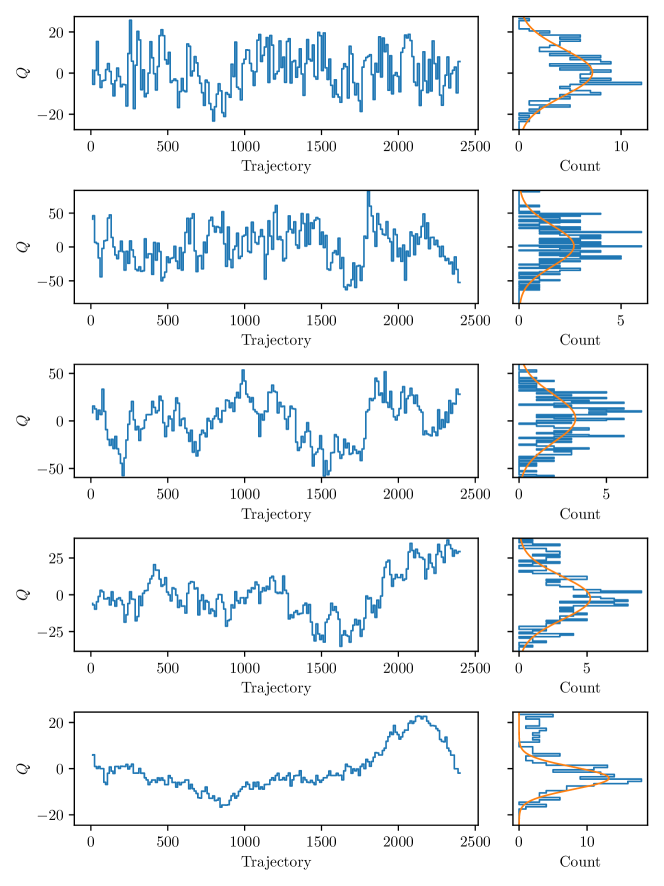
Figure 2: Topological charge histories (left panels), and histograms (right panels), for the five ensembles QB1–QB5, listed from top to bottom. Fitted parameters are given in Table 3. In the plots we show $Q$ evaluated only on the configurations used in the data analysis.

	$Q_{0}$	$\sigma$	$\tau_{\exp}$
QB1	$0.29(92)$	$11.43(94)$	$1.35(21)$
QB2	$1.6(2.3)$	$30.2(2.3)$	$2.95(24)$
QB3	$2.5(2.3)$	$25.4(2.3)$	$7.73(12)$
QB4	$-2.2(1.1)$	$14.7(1.1)$	$15.79(65)$
QB5	$-4.12(46)$	$4.81(46)$	$34.1(1.7)$

Table 3: Fitted parameters from topological charge histories; see also Fig. 2. The autocorrelation time $\tau_{\exp}$ is expressed in units of consecutive configurations.

In numerical lattice calculations, all dimensional quantities can be written in terms of the lattice spacing $a$, for example by defining a dimensionless mass as $m^{\rm latt}=ma$. But in taking the continuum limit, the lattice spacing vanishes, $a\rightarrow 0$. Hence, in order to connect the lattice observables to continuum ones, we have to set a common physical scale that allows the comparison. We adopt as our scale-setting method Lüscher’s gradient-flow (GF) scheme, using the definition of Wilson flow in Ref. Luscher:2010iy (see also Refs. Luscher:2009eq ; Luscher:2011bx ; Fujikawa:2016qis ). This method is particularly suitable for the purpose of this work, since it relies on theoretically defined quantities that do not require direct experimental input.

The scale-setting procedure with the GF scheme in $Sp(4)$ theories has been first discussed in Ref. Bennett:2017kga , both for the pure Yang-Mills and for the theory with two fundamental Dirac fermions (see also Bennett:2017tum ; Bennett:2019jzz ). We follow the same procedure throughout this work: we define the flow scale $w_{0}$ by $\mathcal{W}|_{t=w_{0}^{2}}=\mathcal{W}_{0}$ Borsanyi:2012zs , where $\mathcal{W}(t)$ is the derivative of the action density built from gauge fields at nonzero fictitious flow time $t$. The reference value $\mathcal{W}_{0}=0.35$ has been chosen to minimise both discretisation and finite-volume effects Bennett:2017kga (though with the caveats discussed in Refs. Fodor:2014cpa ; Ramos:2015baa ; Lin:2015zpa ). We also choose a four-plaquette clover for the definition of the field-strength tensors Luscher:2010iy . The resulting values of the flow scale in lattice units $w_{0}/a$ are shown in Table 2.

We measure the history of the topological charge $Q$ to monitor the possible emergence of topological freezing, which might affect spectral measurements Luscher:2011kk ; Galletly:2006hq (see also Refs. Brower:2003yx ; Bernard:2017npd ). Since $Q\equiv\sum_{x}\frac{1}{32\pi^{2}}\epsilon_{\mu\nu\rho\sigma}{\rm Tr\,}\{U_{\mu\nu}(x)U_{\rho\sigma}(x)\}$ is dominated by ultraviolet (UV) fluctuations when calculated directly on the configurations in ensembles QB1–5, configurations that have been smoothed by the gradient flow are instead used. $Q$ is measured at the point in the flow such that the smoothing radius $\sqrt{8t}=L/2$.

In Fig. 2 we present the histories and histograms of $Q$ along the Markov chain for all ensembles in Table 2, the latter of which is fitted with the Gaussian fit form $n(Q)\propto\exp\left(-\frac{(Q-Q_{0})^{2}}{2\sigma^{2}}\right)$. In Table 3 we present the results of this fit, and the exponential autocorrelation time $\tau_{\mathrm{exp}}$ calculated via a fit to the autocorrelation function of $Q$. In the five ensembles, there is no clear evidence of a freeze-out of the topology; the histograms clearly show sampling from multiple topological sectors, and the distributions are peaked within $1\sigma$ of $Q=0$.

However, as we move to finer lattice spacing, we observe that the autocorrelation time of the topological charge grows significantly; in the case of QB5, this has grown to around 34 configurations. In this case specifically $Q_{0}=-4.12$ is also marginal compared to $\sigma=4.81$. This effect may be due to the fact that a change of the discrete global quantity $Q$ by local updates becomes disfavoured in the approach to the continuum limit.

To verify that this increasing $\tau_{\mathrm{exp}}$ and marginal $Q_{0}$ do not affect the spectroscopic results we obtain from these ensembles, we generate an additional ensemble QB$\overline{5}$ of 2400 trajectories starting from the last configuration in QB5. We repeated the measurements of meson masses and decay constants, and of the topological charge history, on 200 configurations sampled from QB$\overline{5}$. While the value of $Q_{0}$ differs between the two ensembles, the meson masses and decay constants do not show significant deviations (beyond the statistical fluctuations). We report these tests in detail in Appendix D. This suggests that any systematic effect associated with the long autocorrelation time of the topological charge and the marginal $Q_{0}$ on the spectroscopy is comfortably smaller than the statistical error for the ensembles and observables we study, and we use ensembles QB1–5 for the remainder of the analysis.

IV Of quenched mesons

In this section, we present the main numerical results of our study. We start by defining the mesonic two-point correlation functions that are computed numerically, and the observables we extract from them, namely the meson masses and decay constants. We provide some technical details about the otherwise standard procedure we follow, in order to clarify how different representations of the gauge group are implemented. Perturbative renormalisation of the decay constants is summarised towards the end of Sec. IV.1. We perform continuum extrapolations with the use of Wilson chiral perturbation theory (W$\chi$PT) in Sec. IV.2. We devote Secs. IV.3 and IV.4 to present the numerical results for the mesons made of fermions transforming in the fundamental and 2-index antisymmetric representations, respectively, and conclude with a comparison of the two representations in Sec. IV.5. For practical reasons, in this section we specify our results to the theory with $N_{f}=2$ fermions on the fundamental representation and $n_{f}=3$ on the antisymmetric, though the results of the quenched calculations apply for generic $N_{f}$ and $n_{f}$.

Label	Interpolating operator	Meson	$J^{P}$	$Sp(4)$	$SO(6)$
$M$	$\mathcal{O}_{M}$	in QCD
PS	$\overline{Q^{i}}\gamma_{5}Q^{j}$	$\pi$	$0^{-}$	$5(+1)$	$1$
S	$\overline{Q^{i}}Q^{j}$	$a_{0}$	$0^{+}$	$5(+1)$	$1$
V	$\overline{Q^{i}}\gamma_{\mu}Q^{j}$	$\rho$	$1^{-}$	$10$	$1$
T	$\overline{Q^{i}}\gamma_{0}\gamma_{\mu}Q^{j}$	$\rho$	$1^{-}$	$10(+5+1)$	$1$
AV	$\overline{Q^{i}}\gamma_{5}\gamma_{\mu}Q^{j}$	$a_{1}$	$1^{+}$	$5(+1)$	$1$
AT	$\overline{Q^{i}}\gamma_{5}\gamma_{0}\gamma_{\mu}Q^{j}$	$b_{1}$	$1^{+}$	$10(+5+1)$	$1$
ps	$\overline{\Psi^{k}}\gamma_{5}\Psi^{m}$	$\pi$	$0^{-}$	$1$	$20^{\prime}(+1)$
s	$\overline{\Psi^{k}}\Psi^{m}$	$a_{0}$	$0^{+}$	$1$	$20^{\prime}(+1)$
v	$\overline{\Psi^{k}}\gamma_{\mu}\Psi^{m}$	$\rho$	$1^{-}$	$1$	$15$
t	$\overline{\Psi^{k}}\gamma_{0}\gamma_{\mu}\Psi^{m}$	$\rho$	$1^{-}$	$1$	$15(+20^{\prime}+1)$
av	$\overline{\Psi^{k}}\gamma_{5}\gamma_{\mu}\Psi^{m}$	$a_{1}$	$1^{+}$	$1$	$20^{\prime}(+1)$
at	$\overline{\Psi^{k}}\gamma_{5}\gamma_{0}\gamma_{\mu}\Psi^{m}$	$b_{1}$	$1^{+}$	$1$	$15(+20^{\prime}+1)$

Table 4: Interpolating operators $\mathcal{O}_{M}$ built of Dirac fermions on the fundamental $Q^{i\,a}$ and antisymmetric $\Psi^{k\,ab}$. We show explicitly the flavour indices $i,j=1\,,\,2$ and $k,m=1\,,\,2\,,\,3$, while colour and spinor indices are implicit and summed over. We also show the $J^{P}$ quantum numbers, the corresponding QCD mesons sourced by the analogous operator, and the irreducible representation of the unbroken global $Sp(4)\times SO(6)$ spanned by the meson (see also Lewis:2011zb ). We indicate in parentheses other nontrivial representations that are obtained with the same operator structure but that we do not study in this paper as they source heavier states. The singlets ($1$ of both $Sp(4)$ and $SO(6)$) are ignored, as we choose to analyse only the operators with $i\neq j$ or $k\neq m$. More details about the symmetries can be found in Appendix E, and the details of a specific choice of basis for the global $SU(4)$ are presented in Appendix F.

IV.1 Correlation functions

We extract masses and decay constants of the lightest flavoured spin-0 and spin-1 mesons from the corresponding Euclidean two-point correlation functions of operators ${\cal O}_{M}$ involving Dirac fermions $Q$ transforming in the fundamental and $\Psi$ in the 2-index antisymmetric representation, as listed in Table 4. In the table, colour and spin indices are implicitly summed over, while the flavour indices $i\neq j$ ($k\neq m$) are chosen. The operators of the form $\overline{Q^{i}}\Gamma_{M}Q^{j}$ are gauge invariant and they source the meson states $M$. Spin and parity $J^{P}$ are determined by the choice of $\Gamma_{M}$. The operators built with $\Gamma=\gamma_{5},\,\gamma_{\mu},\,\gamma_{5}\gamma_{\mu}$, with $\mu=$1, 2, 3, correspond to the pseudoscalar (PS), vector (V), and axial-vectors (AV) mesons, respectively. They appeared in the EFT discussion in Sec II.3. For all of them, we measure both the masses and the decay constants of the particles that they source. For completeness, we also calculate the correlation functions built with $\Gamma=\mathbb{1}_{4},\,\gamma_{0}\gamma_{\mu},\,\gamma_{5}\gamma_{0}\gamma_{\mu}$, which refer to scalar (S), (antisymmetric) tensor (T), and axial tensor (AT), but we extract only the masses of the lightest states sourced by these operators. The operators $\overline{\Psi^{k}}\Gamma_{M}\Psi^{m}$ are defined and classified in the same way, except that we denote them with lowercase letters as ps, v, av, s, t, and at, respectively. In Table 4, we also show the irreducible representation of the unbroken global symmetry $Sp(4)\times SO(6)$, as well as the corresponding mesons in QCD, to provide intuitive guidance to the reader. We also recall that because of the (pseudo)real nature of the representations we use, there is no difference between meson and diquark operators. More details about the classification of the mesons and the relation between four-component and two-component spinors can be found in Appendixes E and F.

The two-point correlation functions at positive Euclidean time $t$ and vanishing momentum $\overrightarrow{p}$ can be written as

$$C_{M,\,M^{\prime}}(t)\equiv\sum_{\vec{x}}\langle 0|\mathcal{O}_{M}(\vec{x},t)\mathcal{O}^{\dagger}_{M^{\prime}}(\vec{0},0)|0\rangle.$$ (42)

We extract physical observables from these objects. In most of our calculations we set $M=M^{\prime}$, with the exception of the extraction of the pseudoscalar decay constant, which involves both ${\cal O}_{\rm PS}$ and ${\cal O}_{\rm AV}$ ( ${\cal O}_{\rm ps}$ and ${\cal O}_{\rm av}$ in the case of fermions $\Psi$). The standard procedure requires rewriting $C(t)$ in terms of fermion propagators $S^{a\alpha}_{\,\,\,\,\,\,\,\,\,b\beta}(x)\equiv\langle Q^{a\alpha}(x)\overline{Q}_{\,b\beta}(0)\rangle$ (and analogous expressions for the propagators involving $\Psi$), to yield

$$C_{M,M^{\prime}}(t)=-\sum_{\vec{x}}{\rm Tr}\left[\Gamma_{M}S(x)\Gamma_{M^{\prime}}\gamma_{5}S^{\dagger}(x)\gamma_{5}\right],$$ (43)

where the trace is over both spinor indices $\alpha,\beta$ and gauge indices $a,b$.

In the simplest case of a point source, the fermion propagator $D^{R}$ ($R$ labeling the fermion representation) is calculated by solving the Dirac equation

$$D^{R}_{a\alpha,b\beta}(x,y)S^{b\beta}_{\,\,\,\,\,\,\,\,c\gamma}(y)=\delta_{x,0}\delta_{\alpha\gamma}\delta_{ac}.$$ (44)

In order to improve the signal, in our numerical studies throughout this work we use the $Z_{2}\times Z_{2}$ single time slice stochastic wall sources Boyle:2008rh with three different sources considered individually for each configuration, instead of the point sources, on the right-hand side of Eq. (44).

In all the spectroscopic measurements using quenched ensembles, we use the (unimproved) Wilson action for the fermions. The corresponding massive Wilson-Dirac operator in the fundamental representation $D^{F}$ is defined by its action on the fermions $Q$, that takes the form

$$D^{F}Q(x)\equiv(4/a+m_{0})Q(x)-\frac{1}{2a}\sum_{\mu} \left\{\frac{}{}(1-\gamma_{\mu})U_{\mu}(x)Q(x+\hat{\mu})\right.+$$ (45)

$$\left.+(1+\gamma_{\mu})U_{\mu}(x-\hat{\mu})Q(x-\hat{\mu})\frac{}{}\right\},$$

where $U_{\mu}(x)$ are the link variables in the fundamental representation of $Sp(4)$, $a$ is the lattice spacing, and $\hat{\mu}$ is the unit vector in the spacelike direction $\mu$.

In order to construct the Dirac operator $D^{AS}$ for fermion fields $\Psi^{ab}$ in the 2-index antisymmetric representation, we follow the prescription in DelDebbio:2008zf . For $Sp(2N)$, we define an orthonormal basis $e_{AS}^{(ab)}$ (with the multi-index $(ab)$ running over ordered pairs with $1\leq a<b\leq 2N$) for the appropriate vector space of $2N\times 2N$ antisymmetric matrices. The $N(2N-1)-1$ such matrices have the following nonvanishing entries. For $b=N+a$ and $2\leq a\leq N$

$$(e_{AS}^{(ab)})_{c,N+c}\equiv-(e_{AS}^{(ab)})_{N+c,c}\equiv\left\{\begin{matrix}&\frac{1}{\sqrt{2\,a\,(a-1)}},~{}~{}~{}\textrm{for}~{}c<a,\\ &\frac{-(a-1)}{\sqrt{2\,a\,(a-1)}},~{}~{}~{}\textrm{for}~{}c=a,\\ \end{matrix}\right.$$ (46)

and for $b\neq N+a$

$$(e_{AS}^{(ab)})_{cd}\equiv\frac{1}{\sqrt{2}}(\delta_{ac}\delta_{bd}-\delta_{bc}\delta_{ad})\,.$$ (47)

The main difference compared to the case of $SU(N)$ is that the base $e_{AS}$ is $\Omega$-traceless, satisfying $\Omega^{dc}\left(e^{(ab)}_{AS}\right)_{cd}=0$. In the $Sp(4)$ case, one can verify that the resulting five nonvanishing matrices satisfy the orthonormalisation condition ${\rm Tr\,}e_{AS}^{(ab)}e_{AS}^{(cd)}=-\delta^{(ab)(cd)}$, while the matrix $e_{AS}^{(13)}$ vanishes identically. The explicit form of the antisymmetric link variables $U^{AS}_{\mu}(x)$ descends from the fundamental link variables $U_{\mu}(x)$, as

$$\left(U^{AS}_{\mu}\right)_{(ab)(cd)}(x)\equiv{\rm Tr}\left[(e_{AS}^{(ab)})^{\dagger}U_{\mu}(x)e_{AS}^{(cd)}U^{\mathrm{T}}_{\mu}(x)\right],~{}~{}~{}{\rm with}~{}a<b,~{}c<d.$$ (48)

Finally, the Dirac operator for the 2-index antisymmetric representation $D^{AS}$ is obtained by replacing $(U_{\mu})_{ab}$ by $(U^{AS}_{\mu})_{(ab)(cd)}$ and $Q$ by $\Psi$ in Eq. (45).

Masses and decay constants for the mesons are extracted from the asymptotic behaviour of $C_{M,\,M^{\prime}}(t)$ at large Euclidean time. We assume it to be dominated by a single mesonic state. If $M=M^{\prime}$, for all meson interpolating operators we can write

$$C_{M,\,M}(t)\xrightarrow{t\rightarrow\infty}\frac{|\langle 0|\mathcal{O}_{M}|M\rangle|^{2}}{2m_{M}}\left[e^{-m_{M}t}+e^{-m_{M}(T-t)}\right],$$ (49)

where $T$ is the temporal extent of the lattice. In our conventions, the meson states $|M\rangle$ are normalised by writing $M=M^{A}T^{A}$, with $T^{A}$ the generators of the global $SU(2N_{f})$ or $SU(2n_{f})$ symmetry. The value of the pseudoscalar decay constant in QCD in these conventions would be $f_{\rm PS}=f_{\pi}\simeq 93\,{\rm MeV}$. We also consider the correlator defined with $M=$ PS and $M^{\prime}=$ AV, for which the large-time behaviour is given by

$$C_{{\rm PS,AV}}(t)\xrightarrow{t\rightarrow\infty}\frac{\langle 0|\mathcal{O}_{\rm AV}|{\rm PS}\rangle\langle 0|\mathcal{O}_{\rm PS}|{\rm PS}\rangle^{*}}{2m_{\rm PS}}\left[e^{-m_{\rm PS}t}-e^{-m_{\rm PS}(T-t)}\right]\,,$$ (50)

having restricted attention to the components of the AV operator with index $\mu=1,2,3$.

We parameterise the vacuum-to-meson matrix elements for fundamental fermions in such a way that the decay constants $f_{M}$ obey the following relations:

$$\langle 0|\mathcal{O}_{\rm AV}|{\rm PS}\rangle = \langle 0|\overline{Q_{1}}\gamma_{5}\gamma_{\mu}Q_{2}|{\rm PS}\rangle\equiv f_{\rm PS}\,p_{\mu},$$

$$\langle 0|\mathcal{O}_{\rm V}|{\rm V}\rangle = \langle 0|\overline{Q_{1}}\gamma_{\mu}Q_{2}|{\rm V}\rangle\equiv f_{\rm V}\,m_{\rm V}\,\epsilon_{\mu},$$

$$\langle 0|\mathcal{O}_{\rm AV}|{\rm AV}\rangle = \langle 0|\overline{Q_{1}}\gamma_{5}\gamma_{\mu}Q_{2}|{\rm AV}\rangle\equiv f_{\rm AV}\,m_{\rm AV}\,\epsilon_{\mu},$$ (51)

where the polarisation vector $\epsilon_{\mu}$ is transverse to the momentum $p_{\mu}$ and normalised by $\epsilon_{\mu}^{*}\epsilon^{\mu}=1$. (For operators constituted by antisymmetric fermions we replace the fields $Q$ by $\Psi$.) For spin-1 V and AV mesons we extract both masses and decay constants from Eqs. (49) and (51). In the case of the pseudoscalar meson, we determine the masses and decay constants by combining Eqs. (49) with $M={\rm PS}$, Eq. (50) and Eq. (51).

The matrix elements at finite lattice spacing $a$ have to be renormalised. For Wilson fermions, the axial and vector currents receive multiplicative (finite) renormalisation. The renormalisation factors $Z_{\rm A}$ and $Z_{\rm V}$ are defined by the relations

$$f_{\rm PS}=Z_{\rm A}f^{\rm bare}_{\rm PS},~{}f_{\rm V}=Z_{\rm V}f^{\rm bare}_{\rm V},~{}f_{\rm AV}=Z_{\rm A}f^{\rm bare}_{\rm AV},$$ (52)

In this work we determine the renormalisation factors via one-loop perturbative matching, and for Wilson fermions the relevant matching coefficients are written as Martinelli:1982mw

$$Z_{\rm A(V)}=1+C(R)(\Delta_{\Sigma_{1}}+\Delta_{\Gamma})\frac{\tilde{g}^{2}}{16\pi^{2}},$$ (53)

where $\Gamma=\gamma_{5}\gamma_{\mu}$ for $Z_{\rm A}$ and $\Gamma=\gamma_{\mu}$ for $Z_{\rm V}$. The eigenvalues of the quadratic Casimir operators with fermions in the fundamental and antisymmetric representations of $Sp(4)$ are $C(F)=5/4$ and $C(AS)=2$, respectively. The matching factors in Eq. (53) are computed by one-loop integrals within the continuum $\overline{\rm MS}$ (modified minimal subtraction) regulalisation scheme. The resulting numerical values are $\Delta_{\Sigma_{1}}=-12.82$, $\Delta_{\gamma_{\mu}}=-7.75$ and $\Delta_{\gamma_{5}\gamma_{\mu}}=-3.0$ Martinelli:1982mw ; Bennett:2017kga . Following the prescription in Ref. Lepage:1992xa , in order to improve the convergence of perturbative expansion we replace the bare coupling $g$ by the tadpole improved coupling defined as $\tilde{g}^{2}=g^{2}/\langle P\rangle$. $\langle P\rangle$ is the average plaquette value, and this procedure removes large tadpole-induced additive renormalisation arising with Wilson fermions.

IV.2 Continuum extrapolation

Extrapolations to the continuum limit are carried out following the same procedure as in Ref. Bennett:2019jzz . We borrow the ideas of tree-level Wilson chiral perturbation theory (W$\chi$PT), which we truncate at the next-to-leading order (NLO) in the double expansion in fermion mass and lattice spacing Sheikholeslami:1985ij ; Rupak:2002sm (see also Ref. Sharpe:1998xm , as well as Symanzik:1983dc ; Luscher:1996sc , though written in the context of improvement). Tree-level results for the full theory can be extended to (partially) quenched calculations, since quenching effects only arise from integrals in fermion loops Rupak:2002sm . But we cannot a priori determine the range of validity of tree-level W$\chi$PT at NLO. On the one hand, if we were too close to the chiral limit, we would need to include loop integrals (the well-known chiral logs). On the other hand, if we were in the heavy mass regime, then we would need to include more higher-order terms. As we will discuss later, most of our data sit somewhere in between these two extrema, and as a consequence we can empirically find appropriate ranges of fermion mass over which tree-level NLO W$\chi$PT well describes the numerical data.

We apply the scale-setting procedure discussed in Sec III.2, and define the lattice spacing in units of the gradient-flow scale as $\hat{a}\equiv a/w_{0}$. All other dimensional quantities are treated accordingly, so that masses are rescaled as in $\hat{m}_{M}\equiv w_{0}m_{M}$ and decay constants as in $\hat{f}_{M}=w_{0}f_{M}$. Tree-level NLO W$\chi$PT assumes that the decay constant squared $\hat{f}_{\rm PS}^{2,{\rm NLO}}$ is linearly dependent on both $\hat{m}_{\rm PS}^{2}$ and $\hat{a}$. We extend this assumption to all other observables as well, hence defining the ansatz

$$\hat{f}_{M}^{2,{\rm NLO}} \equiv \hat{f}_{M}^{2,\chi}\left(1+L_{f,M}^{0}\hat{m}_{\rm PS}^{2}\right)+W_{f,M}^{0}\hat{a}\,,$$ (54)

$$\hat{m}_{M}^{2,{\rm NLO}} \equiv \hat{m}_{M}^{2,\chi}\left(1+L_{m,M}^{0}\hat{m}_{\rm PS}^{2}\right)+W_{m,M}^{0}\hat{a}\,,$$ (55)

for decay constants squared and masses squared, respectively. We note that the fermion mass $m_{f}$ appearing in the standard W$\chi$PT has been replaced by the pseudoscalar mass squared by using LO $\chi$PT results, according to which $\hat{m}_{\rm PS}^{2}=2Bm_{f}$. The low-energy constant $B$ could in principle be determined via a dedicated study of the fermion mass, but this would go beyond our current aims. The empirical prescription we adopt requires us to identify the largest possible region of lattice data showing evidence of the linear behaviour described above and then fit the data in order to identify the additive contribution proportional to $\hat{a}$. Extrapolation to the continuum is obtained by subtracting this contribution from the lattice measurements.

IV.3 Quenched spectrum: Fundamental fermions

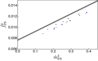
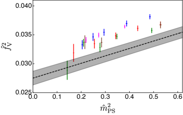
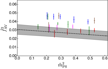
Figure 3: Decay constants squared of PS, V, and AV mesons (constituted of fermions transforming in the fundamental representation), as a function of the PS meson mass squared $\hat{m}^{2}_{\rm PS}$, for $\beta=7.62$ (blue), $7.7$ (purple), $7.85$ (green), $8.0$ (red), and $8.2$ (brown). All quantities are expressed in units of the gradient-flow scale $w_{0}$. The results of the continuum and massless extrapolations are represented by the grey bands.

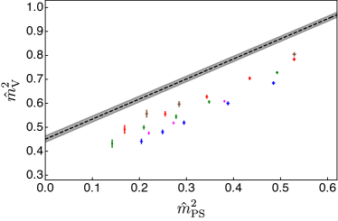
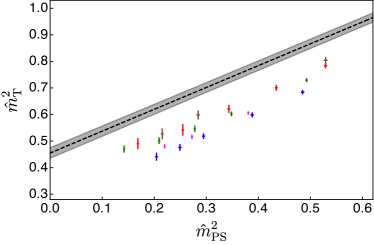
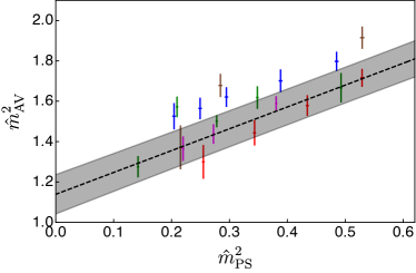
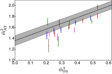
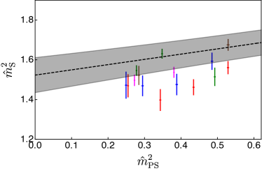
Figure 4: Masses squared of V, T, AV, AT and S mesons (constituted of fermions in the fundamental representation), as a function of the PS meson mass squared $\hat{m}^{2}_{\rm PS}$, for $\beta=7.62$ (blue), $7.7$ (purple), $7.85$ (green), $8.0$ (red), and $8.2$ (brown). All quantities are expressed in units of the gradient-flow scale $w_{0}$. The results of the continuum and massless extrapolations are represented by the grey bands.

Reference Bennett:2017kga reported the quenched spectrum of the lightest PS, V, and AV flavoured mesons for two values of the lattice coupling, $\beta=7.62$ and $8.0$, with fermions in the fundamental representation. In this section, we extend the exploration of the quenched theory in several directions. First, we consider three more values of the coupling, $\beta=7.7$, $7.85$, and $8.2$, as mentioned in Sec III.1, aiming to perform continuum extrapolations, along the lines described in Sec. IV.2. Second, in order to remove potential finite-volume effects, we restrict the bare fermion mass $m_{0}$ to ensembles that satisfy the condition $m_{\rm PS}L\geq 7.5$, in line with the results of the study with dynamical fermions Bennett:2019jzz . Only part of the data in Bennett:2017kga meets this restriction, over the range of $m_{0}\in[-0.7,-0.79]$ at $\beta=7.62$, measured on the lattice with extension $48\times 24^{3}$—corresponding to the ensemble denoted as QB1 in Table 2. For the other values of the lattice coupling we perform new calculations by using lattices with extension $60\times 48^{3}$. The details of all the ensembles are found in Sec III.1 and summarised in Table 2.

For a given ensemble QB$i$ (with $i=1\,,\,\cdots\,,\,5$) we introduce various choices of bare mass $am_{0}$ of the fundamental fermions (see Table 9), and calculate two-point Euclidean correlation functions of pseudoscalar PS, vector V, axial-vector AV, scalar S, (antisymmetric) tensor T and axial-tensor AT meson operators, using the interpolating operators in Table 4. We follow the standard procedure described in Sec IV.1, and we extract the masses and decay constants from the correlated fit of the data for the correlation functions as in Eq. (49). In the case of the pseudoscalar meson, we simultaneously fit the data for the correlators $C_{\rm PS,\,PS}(t)$ and $C_{\rm PS,AV}(t)$ according to Eqs. (49) and (50). The fitting intervals over the asymptotic (plateau) region at large Euclidean time are chosen to optimise the $\chi^{2}$ while keeping the interval as large as possible. Such optimised values are shown in the numerical fits presented in Tables 9 and 10 in Appendix G.

Notice that, in the case of AV, AT and S mesons, we are not able to find an acceptable plateau region for several among the lightest choices of fermion masses. This problem appears when approximately reaching the threshold for decay to three pseudoscalars. Similar problems have been observed before in the literature on quenched theories (see for example Refs. Bernard:1995ez ; Lin:2002aj ; Lin:2003tn ), and may be due to the appearance of two types of new features, both of which are ultimately due to violations of unitarity: polynomial factors correct the exponential behaviour of the large-time correlation functions, and finite-volume effects do not decouple in the infinite-volume limit. We pragmatically decided to ignore measurements showing evidence of these phenomena, and discard them from the analysis.

The resulting values of meson masses and decay constants are presented in Tables 13, 14 and 16 in Appendix G. In Table 13 we also present the results of $m_{\rm PS}\,L$ and $f_{\rm PS}\,L$. For all the listed measurements the lattice volumes are large enough that the finite-volume effects are expected to be negligible as $m_{\rm PS}\,L\mathrel{\raisebox{-2.58334pt}{$\stackrel{{\scriptstyle\textstyle>}}{{\sim}}$}}7.5$, and the low-energy EFT is applicable as $f_{\rm PS}\,L\mathrel{\raisebox{-2.58334pt}{$\stackrel{{\scriptstyle\textstyle>}}{{\sim}}$}}1.6$. All fermion masses are large enough that the decay of a V meson into two PS mesons is kinematically forbidden. The resulting values of the masses measured from the correlators involving $\mathcal{O}_{\rm V}$ and $\mathcal{O}_{\rm T}$ are statistically consistent with each other, in support of theoretical prediction: the V and T operators interpolate the same physical states with $J^{P}=1^{-}$ (identified with the $\rho$ meson in the case of real-world QCD).

We perform simultaneous continuum and massless extrapolations by fitting the data for (quenched) meson masses and decay constants to Eqs. (54) and (55). We restrict the range of masses used for the extrapolations to $\hat{m}_{\rm PS}^{2}\lesssim 0.4$ for the PS states, and to ensembles yielding $\hat{m}_{\rm PS}^{2}\lesssim 0.6$ for all other states, in order to retain the largest possible range of masses within which the data show linear dependence on $\hat{m}_{\rm PS}^{2}$. In Figs. 3 and 4 we show the results of decay constants and masses, with different colours being used to denote ensembles at different $\beta$ values. In the figures we also present the continuum-extrapolated values (denoted by grey bands the widths of which represent the statistical uncertainties), obtained after subtracting artefacts arising from finite lattice spacing. We find that $\hat{f}_{\rm PS}^{2}$, $\hat{m}_{\rm V}^{2}$ and $\hat{m}_{\rm T}^{2}$ are significantly affected by the discretisation of the Euclidian space. And such a long continuum extrapolation can be understood from the fact that we have used the standard Wilson fermions. The size of lattice artefacts in all other quantities is comparable with that of statistical uncertainties.

From the numerical fits we determine the constants appearing in Eqs. (54) and (55), and we report them in Table 5. The numbers in the first and second parentheses are the statistical and systematic uncertainties of the fits, respectively. In the table, we also present the values of $\chi^{2}/N_{\rm d.o.f}$. Some large values of $\chi^{2}/N_{\rm d.o.f}$ indicate that either the uncertainties of the individual data were underestimated or the fit functions are not sufficient to correctly describe the data. Although it would be difficult to fully account for the systematics associated with the continuum extrapolation with limited number of lattice spacings, we estimate the systematic uncertainties in the fits by taking the maximum and minimum values obtained from the set of data excluding the coarsest lattice (the ensemble with $\beta=7.62$) and including or excluding the heaviest measurements. Notice in the table that this process yields large estimates for the systematic uncertainty for those fits that result in a large value of $\chi^{2}/N_{\rm d.o.f}$ at the minimum. Finally, the resulting values in the massless limit, $\hat{f}_{M}^{2,\,\chi}$ and $\hat{m}_{M}^{2,\,\chi}$, should be taken with a due level of caution, since the considered masses are still relatively heavy and only the corrections corresponding to the tree-level terms in the chiral expansion are used in the fits. We leave more dedicated studies of the massless extrapolation to our future work with fully dynamical and light fermions.

As seen in Table 15, for each given value of $\beta$ the ratio $\hat{m}_{\rm V}/\hat{f}_{\rm PS}$ is approximately constant over the mass region $\hat{m}_{\rm V}/\hat{m}_{\rm PS}\mathrel{\raisebox{-2.58334pt}{$\stackrel{{\scriptstyle\textstyle>}}{{\sim}}$}}1.3$. From a simple linear extrapolation to the continuum of these constant vector masses in units of $\hat{f}_{\rm PS}$, we find that $\hat{m}_{\rm V}/\sqrt{2}\hat{f}_{\rm PS}=5.42(5)$. A more rigorous, yet compatible, estimate of the massless limit is obtained by taking the extrapolated results in Table 5 and yields $\hat{m}^{\chi}_{\rm V}/\sqrt{2}\hat{f}^{\chi}_{\rm PS}=5.48(9)(4)$.

	$~{}~{}\hat{f}^{2,\,\chi}_{M}~{}~{}$	$~{}~{}~{}L^{0}_{f,M}~{}~{}~{}$	$~{}~{}~{}~{}~{}W^{0}_{f,M}~{}~{}~{}~{}~{}$	$~{}~{}~{}~{}~{}\chi^{2}/N_{\rm d.o.f}~{}~{}~{}~{}~{}$
PS	$0.00765(13)(11)$	$2.101(38)(51)$	$-0.00190(24)(15)$	$3.1$
V	$0.0275(12)(4)$	$0.47(51)(24)$	$0.0060(18)(4)$	$1.5$
AV	$0.031(6)(10)$	$-0.40(18)(25)$	$0.019(10)(20)$	$4.2$
	$~{}~{}\hat{m}^{2,\,\chi}_{M}~{}~{}$	$~{}~{}~{}L^{0}_{m,M}~{}~{}~{}$	$~{}~{}~{}~{}~{}W^{0}_{m,M}~{}~{}~{}~{}~{}$	$~{}~{}~{}~{}~{}\chi^{2}/N_{\rm d.o.f}~{}~{}~{}~{}~{}$
V	$0.451(13)(5)$	$1.86(7)(4)$	$-0.257(20)(6)$	$0.4$
T	$0.455(20)(7)$	$1.81(8)(5)$	$-0.256(31)(9)$	$0.9$
AV	$1.14(10)(14)$	$0.96(14)(18)$	$0.13(16)(29)$	$3.8$
AT	$1.36(9)(13)$	$0.78(10)(10)$	$-0.19(14)(24)$	$3.1$
S	$1.52(9)(4)$	$0.18(6)(12)$	$-0.14(13)(7)$	$4.0$

Table 5: Results of the fit of the coefficients in Eqs. (54) and (55), used in the continuum and massless extrapolations of masses and decay constants of mesons in the quenched simulations involving Dirac fermions in the fundamental representation. The numbers in parentheses represent, respectively, statistical and systematic uncertainties due to the fit.

IV.4 Quenched spectrum: Antisymmetric fermions

We turn now our attention to the quenched spectrum of the lightest flavoured mesons involving the fermions transforming in the antisymmetric representation of $Sp(4)$. We use the same ensembles listed in Table 2, but the bare masses $m_{0}$ of the fermions are listed in Table 11 of Appendix G. As with fundamental fermions, we choose the values of $am_{0}$ to satisfy the condition of $m_{\rm ps}L\geq 7.5$. In the table, we also present the fitting intervals used for the extraction of the masses and the decay constants of ps, v, av, and s mesons as well as the resulting values of $\chi^{2}/N_{\rm d.o.f}$. The results for t and at mesons are shown in Table 12 of the same appendix. We apply to the antisymmetric case the same numerical treatment and analysis techniques used for the fundamental fermions. As in the case of the fundamental representation, we could not find an acceptable plateau region for some measurements at the smallest fermion masses, in the cases of v, av and s mesons.

In Appendix G we also present the numerical results of the masses and decay constants of ps, v and av mesons, as well as the masses of s, t and at mesons. See Tables 17, 18 and 20. As shown in Table 17, all the measurements meet the aforementioned condition $m_{\rm ps}L\geq 7.5$. In addition, we find that $f_{\rm ps}L\geq 2.3$, which supports the applicability of low-energy EFT techniques. Furthermore, the meson masses in units of $\hat{f}_{\rm ps}$ and the ratio $\hat{f}_{\rm v}/\hat{f}_{\rm ps}$ are presented in Tables 19 and 20. As already seen in the results for fundamental fermions, in all the measurements we find that the results of $\hat{m}_{\rm t}$ are consistent with those of $\hat{m}_{\rm v}$, given the current statistical uncertainties.

We perform the numerical fits of masses and decay constants by using the tree-level NLO W$\chi$PT described by Eqs. (54) and (55). In Figs. 5 and 6, we present the fit results denoted by grey bands as well as numerical results of the masses and the decay constants measured at given lattice parameters. For the fits we consider the same ranges of $\hat{m}_{\rm ps}^{2}$ taken for the case of fundamental fermions: $\hat{m}_{\rm ps}^{2}\lesssim 0.4$ and $\hat{m}_{\rm ps}^{2}\lesssim 0.6$, respectively, for the ps and all other states. Over these mass ranges no significant deviation from linearity of the data in $\hat{a}$ and $\hat{m}_{\rm ps}^{2}$ is visible in our data. Different colours denote different lattice couplings, while the widths of the bands represent the statistical uncertainties of the continuum extrapolations.

The resulting fit values are reported in Table 6. The numbers in the first and second parentheses are the statistical and systematic uncertainties of the fits, respectively. Once more, we estimate the fitting systematics by taking the maximum and minimum values obtained from the set of data excluding the coarsest lattices at $\beta=7.62$ and including or excluding the heaviest measurements.

As in the case of fundamental fermions $Q$, we find that for each $\beta$ value the vector masses in units of the pseudoscalar decay constant are almost constant over the range of $\hat{m}_{\rm v}/\hat{m}_{\rm ps}\mathrel{\raisebox{-2.58334pt}{$\stackrel{{\scriptstyle\textstyle>}}{{\sim}}$}}1.3$—see Table 19. After performing a simple linear extrapolation of these constants, we find that $\hat{m}_{\rm v}/\sqrt{2}\hat{f}_{\rm ps}=4.72(4)$ in the continuum limit. A more rigorous, yet compatible, estimate is obtained by making use of the extrapolated results in Table 6: we find $\hat{m}^{\chi}_{\rm v}/\sqrt{2}\hat{f}^{\chi}_{\rm ps}=4.80(12)(4)$. The resulting value of the ratio is smaller than that for the fundamental fermions by $13\%$.

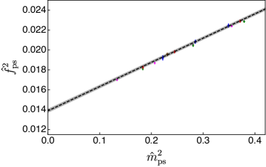
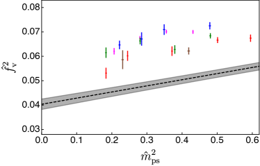
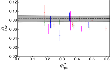
Figure 5: Decay constants squared of ps, v, and av mesons (constituted of fermions in the antisymmetric representation), as a function of the ps meson mass squared $\hat{m}_{\rm ps}^{2}$, for $\beta=7.62$ (blue), $7.7$ (purple), $7.85$ (green), $8.0$ (red), and $8.2$ (brown). All quantities are expressed in units of the gradient-flow scale $w_{0}$. The results of the continuum and massless extrapolations are represented by the grey bands.

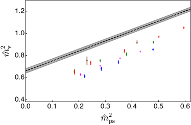
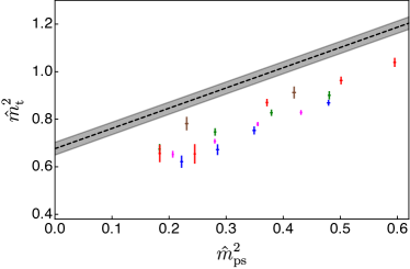
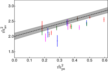
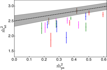
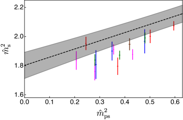
Figure 6: Masses squared of v, t, av, at and s mesons (constituted of fermions transforming in the antisymmetric representation), as a function of the ps meson mass squared $\hat{m}_{\rm ps}^{2}$, for $\beta=7.62$ (blue), $7.7$ (purple), $7.85$ (green), $8.0$ (red), and $8.2$ (brown). All quantities are expressed in units of the gradient-flow scale $w_{0}$. The results of the continuum and massless extrapolations are represented by the grey bands.

	$~{}~{}\hat{f}^{2,\,\chi}_{M}~{}~{}$	$~{}~{}~{}L^{0}_{f,M}~{}~{}~{}$	$~{}~{}~{}~{}~{}W^{0}_{f,M}~{}~{}~{}~{}~{}$	$~{}~{}~{}~{}~{}\chi^{2}/N_{\rm d.o.f}~{}~{}~{}~{}~{}$
ps	$0.01388(18)(10)$	$1.754(41)(28)$	$-0.00028(26)(15)$	$1.3$
v	$0.0404(21)(7)$	$0.626(91)(16)$	$0.0310(28)(17)$	$2.4$
av	$0.084(8)(5)$	$0.01(13)(9)$	$-0.022(12)(9)$	$2.3$
	$~{}~{}\hat{m}^{2,\,\chi}_{M}~{}~{}$	$~{}~{}~{}L^{0}_{m,M}~{}~{}~{}$	$~{}~{}~{}~{}~{}W^{0}_{m,M}~{}~{}~{}~{}~{}$	$~{}~{}~{}~{}~{}\chi^{2}/N_{\rm d.o.f}~{}~{}~{}~{}~{}$
v	$0.657(21)(21)$	$1.375(56)(5)$	$-0.336(34)(4)$	$0.8$
t	$0.675(29)(19)$	$1.26(7)(7)$	$-0.326(47)(19)$	$1.2$
av	$2.01(11)(7)$	$0.70(10)(5)$	$-0.33(17)(11)$	$2.1$
at	$2.50(18)(7)$	$0.32(12)(7)$	$-0.48(24)(8)$	$2.4$
s	$1.80(9)(13)$	$0.32(7)(14)$	$-0.21(12)(15)$	$1.6$

Table 6: Results of the fit of the coefficients in Eqs. (54) and (55), used in the continuum and massless extrapolations of masses and decay constants of mesons in the quenched simulations involving Dirac fermions transforming in the 2-index antisymmetric representation. In parentheses we show statistical and systematic errors, respectively.

IV.5 Quenched spectrum: Comparison

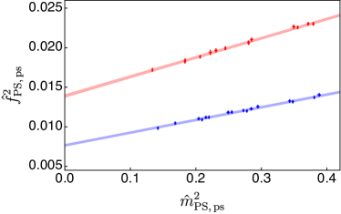
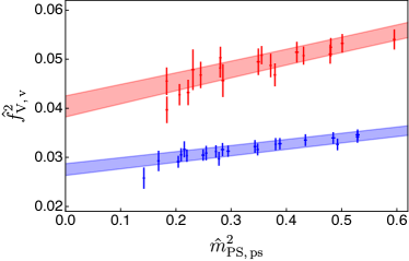
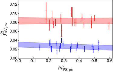
Figure 7: Comparison of the decay constant squared (in the continuum limit) of the mesons as a function of the pseudoscalar meson mass squared, in units of $w_{0}$, for fermion constituents transforming in the fundamental (blue) or 2-index antisymmetric (red) representation.

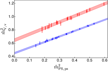
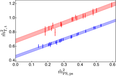
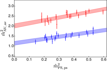
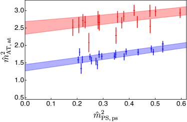
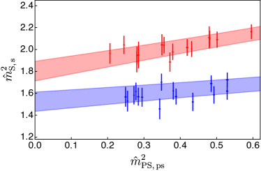
Figure 8: Comparison of the mass squared (in the continuum limit) of the mesons as a function of the pseudoscalar meson mass squared, in units of $w_{0}$, for fermion constituents transforming in the fundamental (blue) or 2-index antisymmetric (red) representation.

Fig. 7 shows a visual comparison between the decay constants of the pseudoscalar, vector, and axial-vector mesons, made of fermions transforming in the fundamental representation of $Sp(4)$ (PS, V, AV) and in the 2-index antisymmetric representation (ps, v, av). In order to make the comparison, we plot the continuum-limit results by naively identifying the masses of the pseudoscalars $\hat{m}_{\rm PS}^{2}=\hat{m}_{\rm ps}^{2}$ as the abscissa. The comparison at finite mass should be taken with some caution, as the symmetry-breaking operators controlling the mass of PS and ps states are distinct, but the massless extrapolations can be compared unambiguously. We repeat the exercise also for the masses of all the mesons, and show the result in Fig. 8.

In all cases we considered, masses and decay constants of bound states made of fermions $\Psi$ transforming in the 2-index antisymmetric representation are considerably larger than those made of fermions $Q$ transforming in the fundamental representation. Focusing on the massless limit, we find that the ratio $\hat{f}_{\rm av}^{2}/\hat{f}_{\rm AV}^{2}=2.7\pm 1.1$ is the largest, while $\hat{m}_{\rm s}^{2}/\hat{m}_{\rm S}^{2}=1.18\pm 0.13$ is the smallest, and the other results are distributed in the range between these two values. The hierarchy between the pseudoscalar decay constants is important in the CHM context; we find that $\hat{f}_{\rm ps}^{2}/\hat{f}_{\rm PS}^{2}=1.81\pm 0.04$. It is also to be noted that the mass of the vector states v is larger, but not substantially so, in respect to that of the corresponding V mesons, with $\hat{m}_{\rm v}^{2}/\hat{m}_{\rm V}^{2}=1.46\pm 0.08$.

How much of the above holds true for the dynamical calculations is not known and is an interesting topic for future studies. It was shown in Ref. Bennett:2019jzz that, by comparing quenched and dynamical calculations for mesons in the fundamental representation (performed in comparable ranges of fermion mass), and after both the continuum and massless extrapolations were performed, the discrepancies are not too large: ${\cal O}(25\%)$ for $\hat{m}_{\rm S}^{2}$, ${\cal O}(20\%)$ for $\hat{f}_{\rm PS}^{2}$, ${\cal O}(10\%)$ for $\hat{m}_{\rm V}^{2}$, and smaller for the other measurements. Whether this is due to the fact that all the calculations in Ref. Bennett:2019jzz are performed in a range of fermion masses that are comparatively large or to other reasons—the large-$N$ behaviour of the theory might already be dominating the dynamics of $Sp(4)$ mesons, for example—is not currently known and should be studied in future dedicated investigations. Yet, it is suggestive that no dramatic discrepancy has emerged so far, for all the observables we considered.

We conclude this section by reminding the reader that the calculations performed for this paper, being done with the quenched approximation, are insensitive to the number of fundamental flavours $N_{f}$ and antisymmetric flavours $n_{f}$ and hence apply to other models, beyond the phenomenologically relevant case with $N_{f}=2$ and $n_{f}=3$. A recent lattice study within the $SU(3)$ gauge theory Nogradi:2019iek of the ratio $m_{\rho}/f_{\pi}$ between the mass of the rho mesons and the decay constant of the pions (corresponding to $m_{\rm V}/f_{\rm PS}$ in this paper) shows no appreciable dependence on the number of flavours $N_{f}\mathrel{\raisebox{-2.58334pt}{$\stackrel{{\scriptstyle\textstyle<}}{{\sim}}$}}6$—as long as the theory is deep inside the regime in which chiral symmetry breaking occurs. It would be interesting to measure whether this holds true also for other representations, in the dynamical theories. Meanwhile, we find that in our quenched calculation, after taking both the continuum and massless limits, for the fundamental representation we have $\hat{m}_{\rm V}^{2}/\hat{f}_{\rm PS}^{2}=59.0\pm 2.2$, while for the antisymmetric representation we find $\hat{m}_{\rm v}^{2}/\hat{f}_{\rm ps}^{2}=47.3\pm 2.3$. The discrepancy reaches beyond the $3\sigma$ level, suggesting that this ratio—which enters into the Kawarabayashi-Suzuki-Riazuddin-Fayyazuddin (KSRF) relation $M_{\rho}^{2}/(g_{\rho\pi\pi}^{2}f_{\pi}^{2})=2$ Kawarabayashi:1966kd ; Riazuddin:1966sw —depends on the fermion representation. By comparison, the ratio obtained from the numerical studies with dynamical Dirac fermions in the fundamental representation is $\hat{m}_{V}^{2}/\hat{f}_{PS}^{2}=65.4\pm 5.0$ Bennett:2019jzz , which is slightly larger than the result of our quenched calculation. Once more, checking this result (as well as the KSRF relations) in the full dynamical theory with fermions in the antisymmetric representation would be of great interest.

V Global fits

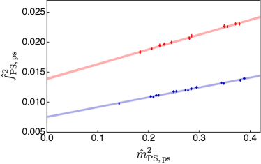
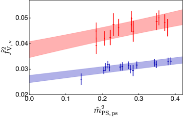
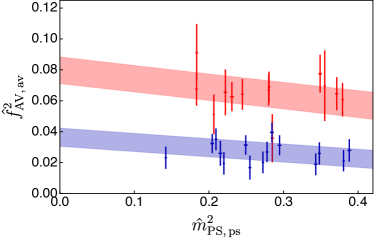
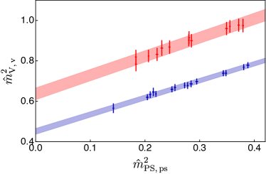
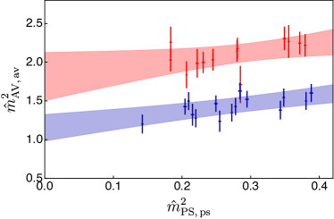
Figure 9: Decay constants and masses in the continuum limit after subtracting lattice artefacts due to the finite lattice spacing. The global fit results are denoted by blue solid bands for the mesons constituted of fundamental fermions $Q$, and red bands for the ones constituted of antisymmetric fermions $\Psi$. The width of the bands indicates the statistical errors.

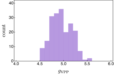
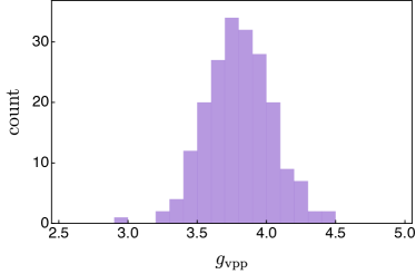
Figure 10: Histogram distribution of the $g_{VPP}$ (left panel) and $g_{vpp}$ (right panel) couplings, obtained from the quenched calculation by applying the global fit strategy discussed in the text. In the former, $g_{VPP}$ denotes the coupling between mesons composed of fermions in the fundamental. In the latter case the constituent fermions transform in the 2-index antisymmetric representation.

In this section, we perform a global fit of the continuum-extrapolated masses and decay constants of PS, V, and AV mesons to the EFT described in Sec. II.3. As stated there, the EFT equations are applicable both to mesons constituted of fermions in the fundamental as well as 2-index antisymmetric representations of the $Sp(4)$ gauge group. We also recall from Ref. Bennett:2017kga that several working assumptions have been used to arrive at Eqs. (33)–(38). We follow in the analysis the prescription introduced in Ref. Bennett:2019jzz . We only repeat some of the essential features of the process, while referring the reader to Ref. Bennett:2019jzz for details. We focus instead on the results of the global fit.

We start by restricting the data analysed to lie in the mass range over which all the measured masses and decay constants can be extrapolated to the continuum limit using Eqs. (54) and (55). In the case of the fundamental representation, we restrict our measurements to include only QB1FM3$-$QB1FM6, QB2FM1$-$QB2FM3, QB3FM4$-$QB3FM7, QB4FM6$-$QB4FM8, and QB5FM2$-$QB5FM3. In the case of antisymmetric representation, we restrict to QB1ASM4$-$QB1ASM6, QB2ASM3$-$QB2ASM6, QB3ASM2$-$QB3ASM4, QB4ASM4$-$QB4ASM6, and QB5ASM2. As anticipated in Sec IV.2, we use the LO $\chi$PT result for the pseudoscalar mass, and replace the fermion mass in Eqs. (33)–(38) by $\hat{m}_{\rm PS}^{2}=2Bm_{f}$. In the mass range considered, this replacement is supported by the numerical data, as $\hat{m}_{\rm PS}^{2}$ is found to be approximately linear with the mass of the fermion $\hat{m}_{0}$. Accordingly, we expand the EFT equations and truncate at the linear order in $\hat{m}_{\rm PS}^{2}$. The resulting fit equations have been presented as Eqs. (6.1)–(6.5) in Ref. Bennett:2019jzz . The ten unknown low-energy constants, denoted as $(\hat{f},~{}\hat{F},~{}b,~{}c,~{}g_{V}~{},\kappa,~{}\hat{v}_{1},~{}\hat{v}_{2},~{}\hat{y}_{3},~{}\hat{y}_{4})$, are appropriately redefined by introducing the gradient-flow scale $w_{0}$.

We perform the numerical global fits of the data to the EFTs, via standard $\chi^{2}$ minimisation, by using $200$ bootstrapped samples and a simplified $\chi^{2}$ function that is built by just summing the individual $\chi^{2}$ functions for the five independent fit equations. The fit results satisfy the constraints obtained from the unitarity conditions in Eq. (6.8) of Ref. Bennett:2019jzz . In practice, we guide the fits by an initial minimisation of the full dataset. In Fig. 9 we present the results of the global fit along with the continuum-extrapolated data used for the fits, by further comparing the results originating from fundamental and antisymmetric fermions. In the figure, the fit results are presented by shaded bands, the widths of which represent the statistical uncertainties. The quality of the fits is measured by the fact that $\chi^{2}/N_{\rm d.o.f}\sim 0.6$ at the minimum, although one should remember that correlations have not been taken into consideration in the analysis. The results of continuum and massless extrapolations, displayed in Figs. 7 and 8, are in good agreement, even in proximity of the massless limit, with those of this alternative analysis.

As pointed out in Ref. Bennett:2019jzz , some of the parameters in the EFTs are not well constrained by the global fit of measurements coming from two-point functions only. Hence, we do not report the individual best-fit results, which are affected by flat directions and large correlations. Yet, in the same reference it is observed that some (nontrivial) combinations of the parameters may be determined well. One of the most interesting such quantities is the coupling constant associated with the decay of a vector meson V (or v) into two pseudoscalar mesons PS (ps). These couplings play the same role as the $g_{\rho\pi\pi}$ in low-energy QCD. The resulting values in the cases of fundamental and antisymmetric fermions are

$$g_{\rm VPP}^{\chi}=4.95(21)(8)~{}~{}~{}{\rm and}~{}~{}~{}g_{\rm vpp}^{\chi}=3.80(24)(16),$$ (56)

respectively, where the suffix ${\chi}$ denotes the result of simultaneous continuum and massless extrapolations. As shown in Fig. 10, the distributions of this quantity exhibit a regular Gaussian shape, from which we estimate the statistical uncertainty—the numbers in the first parentheses of Eq. (56). The numbers in the second parentheses in Eq. (56) denote the systematic errors of the fits with similar caveats to those discussed in Sec IV.3, that we estimated by taking the maximum and minimum values obtained from the set of data excluding the coarsest ensemble and including or excluding the heaviest measurements.

The EFT analyses performed in this section is affected by several limitations—in particular by the quenched approximation and by the comparatively large fermion masses—and thus one should interpret the results with some caution. Yet, it is interesting to compare the EFT results with phenomenological models and with available measurements obtained with dynamical fermions transforming in the fundamental representation. We first compare the EFT results in Eq. (56) with the ones predicted from the KSRF relation, $g_{\rm VPP}=m_{\rm V}/\sqrt{2}m_{\rm PS}$. We find that the left-hand side is smaller than the right-hand side of this relation by about $10\%$ and $23\%$, for the fundamental and antisymmetric representations, respectively. These discrepancies are larger than the uncertainties associated with the fits, and might indicate that the KSRF relation does not describe the quenched theories accurately, particularly in the case of the antisymmetric representation, although this statement is affected by uncontrolled systematic uncertainties due to the use of the EFT with such large values of $g_{\rm VPP}$ and $g_{\rm vpp}$, as well as large fermion masses. We also find that for the fundamental representation the quenched value of $g_{\rm VPP}^{\chi}$ is smaller by $29\%$ compared to the dynamical value of $g_{\rm VPP}^{\chi}=6.0(4)(2)$ Bennett:2019jzz , yielding again a discrepancy that is significantly larger than the fit uncertainties. It would be interesting to repeat these tests with dynamical fermions in the antisymmetric representation, and in general to explore more directly the low-mass regimes of all these theories, but these are tasks that we leave for future extensive studies.

VI Conclusions and Outlook

Composite Higgs and (partial) top compositeness emerge naturally as the low-energy EFT description of gauge theories with fermion matter content in mixed representations of the gauge group. Motivated by this framework, we considered the $Sp(4)$ gauge theory with $N_{f}$ quenched Wilson-Dirac fermions $Q$ transforming in the fundamental representation of $Sp(4)$, as well as $n_{f}$ quenched fermions $\Psi$ in the 2-index antisymmetric representation. While the quenched theory is not expected to reproduce the full dynamics, it provides a useful comparison case for future full dynamical calculations. We generated lattice ensembles consisting of gauge configurations by means of the HB algorithm, modified appropriately the HiRep code DelDebbio:2008zf , considered meson operators ${\cal O}_{M}$ bilinear in these fermions (see Table 4 for explicit definitions of the operators), and measured two-point Euclidean correlation functions of such operators on discrete lattices (and in the quenched approximation).

We hence extracted decay constants $f_{M}$ and masses $m_{M}$ of the flavoured mesons sourced by the operators ${\cal O}_{M}$, with $M=$ PS, V, AV, S, T, and AT (and $M=$ ps, v, av, s, t, and at), defined in Table 4. We renormalised the decay constants, expressed all dimensional quantities in terms of the gradient-flow scale $w_{0}$, and—having restricted attention to ensembles for which finite-volume effects can be ignored—applied tree-level W$\chi$PT to extrapolate toward the continuum and massless limits the results for mesons constituted of both fermion species. We also performed a first global fit of the continuum results that makes use of the EFT describing the lightest spin-1 states (besides the pseudoscalars). It is constructed by extending with the language of hidden local symmetry the chiral-Lagrangian description of the pNGBs spanning the $SU(2N_{f})\times SU(2n_{f})/Sp(2N_{f})\times SO(2n_{f})$ coset.

Our main results for the physical observables in the continuum limit are listed in the tables and plots in Secs. IV.3 and IV.4 and graphically illustrated in Sec. IV.5 (see in particular Figs. 7 and 8). They can be summarised as follows. In the quenched approximation, after extrapolation to the massless limit, all dimensional quantities extracted from two-point correlation functions involving operators constituted of $\Psi$ fermions are larger than the corresponding observables involving $Q$ fermions. The two extremes are $\hat{m}_{\rm s}^{2}/\hat{m}_{\rm S}^{2}=1.18\pm 0.13$ and $\hat{f}_{\rm av}^{2}/\hat{f}_{\rm AV}^{2}=2.7\pm 1.1$, respectively, with all other ratios between observables in the two sectors falling between these two values. (Of particular interest for model building are the ratios $\hat{m}_{\rm v}^{2}/\hat{m}_{\rm V}^{2}=1.46\pm 0.08$ and $\hat{f}_{\rm ps}^{2}/\hat{f}_{\rm PS}^{2}=1.81\pm 0.04$.) The error bars comprise both statistical as well as systematic errors, the latter arising from the continuum and massless extrapolations as discussed in details in Sec IV. Furthermore, we found statistically significant violations of the KSRF relations by the mesons made of antisymmetric fermions, at least in the quenched approximation. (The extraction of the $g_{\rm VPP}$ and $g_{\rm vpp}$ couplings from the global fit of two-point function data collected with large fermion mass to the EFT is affected by unknown systematic effects, and hence this should be taken as a preliminary result.)

Despite the physical limitations of the studied quenched theory, this paper opens the way toward addressing a number of interesting questions in future related work, a first class of which is related to the comparison of the quenched calculations to the full dynamical ones, in particular for the case of fermions in the antisymmetric representation. While it was observed elsewhere Bennett:2019jzz that the quenched approximation captures remarkably well the dynamics of fundamental fermions (at least for the range of masses hitherto explored), there is no clear reason for this to happen also in the antisymmetric case, for which large-$N$ arguments are less constraining. In order to address this point, one would require to study the dynamical simulations with $\Psi$ fermions, in the phenomenologically relevant low-mass ranges of the dynamical calculations, and also to generalise our approach to $Sp(2N)$ gauge theories. The reader may be aware of the possibility that, with higher-dimensional representations and large numbers of fermion degrees of freedom, some of the $Sp(2N)$ theories we are interested in might be close to the edge of the conformal window and behave very differently. (For perturbative studies within the $Sp(2N)$ class, see for instance Refs. Sannino:2009aw ; Ryttov:2017dhd ; Kim:2020yvr , and references therein.)

The extensive line of research outlined in the previous paragraph complements the development of our programme of studies in the context of top compositeness, that as outlined in Ref. Bennett:2017kga requires one to consider the dynamical theory in the presence of mixed representations. This is a novel area of exploration for lattice gauge theories, for which the literature is somewhat limited (see for instance Refs. DeGrand:2016pgq ; Ayyar:2017qdf ; Ayyar:2018zuk ; Ayyar:2018glg ; Cossu:2019hse ). New fermion bound states, sometimes referred to as chimera baryons, can be sourced by operators that involve gauge-invariant combinations of fermions in mixed representations. (The anomalous dimensions of chimera baryons are discussed for example in DeGrand:2015yna ; Cacciapaglia:2019dsq ; BuarqueFranzosi:2019eee .) The study of these states is necessary in the context of top compositeness, as they are interpreted as top partners.

A third group of future research projects can be envisioned to explore the role of higher-dimensional operators, for which the material in the Appendixes of this paper is technically useful. These operators play a role in determining the physics of vacuum (mis)alignment and of electroweak symmetry breaking, as their matrix elements enter the calculation of the potential in the low-energy EFT description. These studies would provide an additional link to phenomenological investigations of composite Higgs models, bringing lattice calculations in close contact with model-building considerations and searches for new physics at the Large Hadron Collider (LHC).

Finally, it would be interesting to investigate the finite temperature behaviour of these theories. As discussed in Appendix E.1, it is important to characterise symmetry restoration and symmetry enhancement that appear at high temperature, generalising what has been studied about QCD to the case of real and pseudoreal representations, for which the group structure of the global symmetries and their breaking is expected to be different.

We acknowledge useful discussions with Axel Maas, Roman Zwicky and Daniel Nogradi.

The work of E.B., M.M., and J.R. has been funded in part by the Supercomputing Wales project, which is part funded by the European Regional Development Fund (ERDF) via Welsh Government.

The work of D.K.H. was supported by Basic Science Research Program through the National Research Foundation of Korea (NRF) funded by the Ministry of Education (NRF-2017R1D1A1B06033701).

The work of J.-W.L. is supported in part by the National Research Foundation of Korea grant funded by the Korea government(MSIT) (NRF-2018R1C1B3001379) and in part by Korea Research Fellowship programme funded by the Ministry of Science, ICT and Future Planning through the National Research Foundation of Korea (2016H1D3A1909283).

The work of C.-J.D.L. is supported by the Taiwanese MoST Grant No. 105-2628-M-009-003-MY4.

The work of B.L. and M.P. has been supported in part by the STFC Consolidated Grants ST/L000369/1 and ST/P00055X/1. B.L. and M.P. received funding from the European Research Council (ERC) under the European Union’s Horizon 2020 research and innovation programme under Grant Agreement No 813942. The work of B.L. is further supported in part by the Royal Society Wolfson Research Merit Award N0. WM170010.

J.R. acknowledges support from Academy of Finland Grant 320123

D.V. acknowledges support from the INFN HPC-HTC project.

Numerical simulations have been performed on the Swansea SUNBIRD system, on the local HPC clusters in Pusan National University (PNU) and in National Chiao-Tung University (NCTU), and on the Cambridge Service for Data Driven Discovery (CSD3). The Swansea SUNBIRD system is part of the Supercomputing Wales project, which is part funded by the European Regional Development Fund (ERDF) via Welsh Government. CSD3 is operated in part by the University of Cambridge Research Computing on behalf of the STFC DiRAC HPC Facility (www.dirac.ac.uk). The DiRAC component of CSD3 was funded by BEIS capital funding via STFC capital Grants No. ST/P002307/1 and No. ST/R002452/1 and STFC operations Grant No. ST/R00689X/1. DiRAC is part of the National e-Infrastructure.

Appendix A Spinors

We summarise in this Appendix our conventions in the treatment of spinors, which are useful, for example, in switching between the two-component and the four-component notation (see also Ref. Lee:2017uvl ). The former is best suited to highlight the symmetries of the system, while the latter is the formalism adopted as a starting point for the lattice numerical treatment. We highlight some important symmetry aspects that offer insight in the theories studied in this paper.

For two-component spinors, we use the Pauli matrices, denoted as $\tau^{i}$, with $i=1,2,3$, and

$$\tau^{1} = \left(\begin{array}[]{cc}0&1\cr 1&0\end{array}\right)\,,\,\tau^{2}\,=\,\left(\begin{array}[]{cc}0&-i\cr i&0\end{array}\right)\,,\,\tau^{3}\,=\,\left(\begin{array}[]{cc}1&0\cr 0&-1\end{array}\right)\,.$$ (63)

Given a two-component spinor $u$, with no internal quantum numbers, we define the ${\cal C}$-conjugate $u_{C}\equiv i\tau^{2}u^{\ast}\equiv-\tilde{C}u^{\ast}$. Furthermore, we introduce the notation $\sigma^{\mu}\equiv(\mathbb{1}_{2},-\tau^{i})$ and $\bar{\sigma}^{\mu}\equiv(\mathbb{1}_{2},\tau^{i})$.

We adopt conventions in which the space-time Minkowski metric is

$$\eta_{\mu\nu}\equiv\,\left(\begin{array}[]{cccc}1&&&\cr&-1&&\cr&&-1&\cr&&&-1\cr\end{array}\right)\,=\,\eta^{\mu\nu}\,.$$ (68)

The Dirac algebra is defined by the anticommutation relation

$$\{\gamma^{\mu},\gamma^{\nu}\}=2\eta^{\mu\nu}\,,$$ (69)

with the $4\times 4$ matrix $\gamma^{0}$ Hermitian, while the three $\gamma^{i}$ are anti-Hermitian, so that $\gamma^{0}\gamma^{\mu}\gamma^{0}=\gamma^{\mu\,\dagger}$. Chirality is defined by the eigenvalues of the matrix $\gamma_{5}\equiv i\gamma^{0}\gamma^{1}\gamma^{2}\gamma^{3}$, that satisfies the relation $\{\gamma^{\mu}\,,\,\gamma^{5}\}=0$.

The charge-conjugation matrix $C=i\gamma^{2}\gamma^{0}$ obeys the defining relations $C\gamma^{\mu}C^{-1}=-\gamma^{\mu\,\mathrm{T}}$ and $C^{2}=-\mathbb{1}_{4}=-CC^{\dagger}$. The chiral representation of the $\gamma^{\mu}$ matrices is

$$\gamma^{0} = \left(\begin{array}[]{cc}0&\mathbb{1}_{2}\cr\mathbb{1}_{2}&0\end{array}\right)\,,~{}~{}\gamma^{i}\,=\,\left(\begin{array}[]{cc}0&-\tau^{i}\cr\tau^{i}&0\end{array}\right)\,,~{}~{}\gamma^{5}\,=\,\left(\begin{array}[]{cc}\mathbb{1}_{2}&0\cr 0&-\mathbb{1}_{2}\end{array}\right)\,,~{}~{}C\,=\,\left(\begin{array}[]{cc}-i\tau^{2}&0\cr 0&i\tau^{2}\end{array}\right)\,,$$ (78)

which implies the useful relations

$$\gamma^{0}\gamma^{\mu} = \left(\begin{array}[]{cc}\bar{\sigma}^{\mu}&0\cr 0&\sigma^{\mu}\end{array}\right)\,,~{}~{}~{}C\gamma^{0}\gamma^{\mu}C^{-1}\,=\,\left(\begin{array}[]{cc}{\sigma}^{\mu}&0\cr 0&\bar{\sigma}^{\mu}\end{array}\right)\,.$$ (83)

We also define the matrices

$$\sigma^{\mu\nu} \equiv \frac{i}{2}\left[\gamma^{\mu}\frac{}{},\,\gamma^{\nu}\right]\,,$$ (84)

which obey the relations $\left[\gamma_{5}\,,\,\sigma^{\mu\nu}\right]=0$, $\gamma^{0}\sigma^{\mu\nu}\gamma^{0}=(\sigma^{\mu\nu})^{\dagger}$ and $\gamma_{5}\sigma^{\mu\nu}=\frac{i}{2}\epsilon^{\mu\nu\rho\sigma}\sigma_{\rho\sigma}$, where $\epsilon^{\mu\nu\rho\sigma}$ is the completely antisymmetric Levi-Civita symbol. In the chiral representation for the $\gamma^{\mu}$ matrices, the six $\sigma^{\mu\nu}$ matrices are block diagonal and can be written as

$$\sigma^{\mu\nu} = \,\left(\begin{array}[]{cc}\sigma^{\mu\nu}_{LL}&0\cr 0&\sigma^{\mu\nu}_{RR}\end{array}\right)\,,~{}~{}~{}~{}\sigma^{\mu\nu}\gamma_{5}\,=\,\,\left(\begin{array}[]{cc}\sigma^{\mu\nu}_{LL}&0\cr 0&-\sigma^{\mu\nu}_{RR}\end{array}\right)\,=\gamma_{5}\sigma^{\mu\nu}\,.$$ (89)

By isolating the spatial indices $i$, one finds that

$$\sigma^{0i} = i\,\left(\begin{array}[]{cc}\tau^{i}&0\cr 0&-\tau^{i}\end{array}\right)\,,~{}~{}~{}~{}\sigma^{ij}\,=\,\epsilon^{ijk}\,\left(\begin{array}[]{cc}\tau^{k}&0\cr 0&\tau^{k}\end{array}\right)\,.$$ (94)

We introduce the notation $\bar{\lambda}\equiv\lambda^{\dagger}\gamma^{0}$. A single Majorana spinor $\lambda$ obeys the relation $\lambda=\pm\lambda_{C}\equiv\pm C\bar{\lambda}^{\mathrm{T}}\equiv\pm C\gamma^{0}\lambda^{\ast}=\pm i\gamma^{2}\lambda^{\ast}$. We conventionally resolve the $\pm$ ambiguity by the choice of the $+$ sign. Starting from a two-component spinor $u$, a four-component Majorana spinor is

$$\lambda = \left(\begin{array}[]{c}u\cr i\tau^{2}u^{\ast}\equiv-\tilde{C}u^{\ast}\end{array}\right)\,,$$ (97)

so that $\lambda=\lambda_{C}$. The left-handed (LH) chiral projector is $P_{L}=\frac{1}{2}\left(\mathbb{1}_{4}+\gamma_{5}\right)$, so that a four-component LH chiral spinor $\lambda_{L}=P_{L}\lambda$ satisfies $P_{L}\lambda_{L}=\lambda_{L}$. Analogous definitions apply to the right-handed (RH) projector $P_{R}$ and spinor $\lambda_{R}$. The decomposition in LH and RH four-components chiral Weyl spinors is given by

$$\lambda_{L} = \left(\begin{array}[]{c}u\cr 0\end{array}\right)\,,~{}~{}~{}~{}~{}\lambda_{R}\,=\,\left(\begin{array}[]{c}0\cr i\tau^{2}u^{\ast}\equiv-\tilde{C}u^{\ast}\end{array}\right)\,,$$ (102)

and yields the relations $\lambda_{L}=C\overline{\lambda_{R}}^{\,\,\mathrm{T}}$ and $\overline{\lambda_{L}}=\lambda_{R}^{\,\,\mathrm{T}}C=-\lambda_{R}^{\,\,\mathrm{T}}C^{-1}$. Clearly, $u$, $\lambda$, $\lambda_{L}$ and $\lambda_{R}$ are different ways to encode the same information.

Consider two distinct, two-component spinors $u$ and $d$, with no additional internal degrees of freedom (aside from the spinor index $\alpha=1,2$). When taken together, they naturally define the fundamental representation of a global $U(2)$ symmetry. Their components are described by Grassmann variables, satisfying the two nontrivial relations

$$u^{\alpha\,\ast}d^{\beta}\,=\,-d^{\beta}u^{\alpha\,\ast}\,,~{}~{}~{}~{}\Big{(}u^{\alpha\,\ast}d^{\beta}\Big{)}^{\ast}\,=\,d^{\beta\,\ast}u^{\alpha}\,,$$ (103)

and analogous for all other combinations.

A Dirac four-component spinor is obtained by joining the LH projection of the Majorana spinor built starting from $u$ and the RH projection of the Majorana spinor corresponding to $d$, so that $Q=U_{L}+D_{R}$ with

$$U_{L} \equiv \left(\begin{array}[]{c}u\cr 0\end{array}\right)\,,~{}~{}~{}~{}D_{R}\,\equiv\,\left(\begin{array}[]{c}0\cr-\tilde{C}d^{\ast}\end{array}\right)\,,~{}~{}~{}~{}D_{L}\,\equiv\,\left(\begin{array}[]{c}d\cr 0\end{array}\right)\,,~{}~{}~{}~{}U_{R}\,\equiv\,\left(\begin{array}[]{c}0\cr-\tilde{C}u^{\ast}\end{array}\right)\,,$$ (112)

and $Q_{C}\equiv C\overline{Q}^{\mathrm{T}}=C\gamma^{0}Q^{\ast}=D_{L}\,+\,U_{R}$, while $\overline{Q_{C}}=Q^{\mathrm{T}}C$.

By inspection, one finds that the following relations hold true:

$$\overline{Q}P_{L}Q = \overline{D_{R}}U_{L}\,=\,d^{\mathrm{T}}\tilde{C}u\,,~{}~{}~{}~{}(\overline{Q}P_{L}Q)^{\ast}\,=\,\overline{Q}P_{R}Q\,=\,-u^{\dagger}\tilde{C}d^{\ast}\,,$$

$$\overline{Q_{C}}P_{L}Q_{C} = \overline{U_{R}}D_{L}\,=\,u^{\mathrm{T}}\tilde{C}d\,,~{}~{}~{}~{}(\overline{Q_{C}}P_{L}Q_{C})^{\ast}\,=\,\overline{Q_{C}}P_{R}Q_{C}\,=\,-d^{\dagger}\tilde{C}u^{\ast}\,,$$

$$\overline{Q}P_{L}Q_{C} = \overline{D_{R}}D_{L}\,=\,d^{\mathrm{T}}\tilde{C}d\,,~{}~{}~{}~{}(\overline{Q}P_{L}Q_{C})^{\ast}\,=\,\overline{Q_{C}}P_{R}Q\,=\,-d^{\dagger}\tilde{C}d^{\ast}\,,$$ (113)

$$\overline{Q_{C}}P_{L}Q = \overline{U_{R}}U_{L}\,=\,u^{\mathrm{T}}\tilde{C}u\,,~{}~{}~{}~{}(\overline{Q_{C}}P_{L}Q)^{\ast}\,=\,\overline{Q}P_{R}Q_{C}\,=\,-u^{\dagger}\tilde{C}u^{\ast}\,,$$

and by using the $\gamma^{\mu}$ matrices, one also finds the relations

$$\overline{Q}\gamma^{\mu}P_{L}Q = \overline{U_{L}}\gamma^{\mu}U_{L}\,=\,u^{\dagger}\bar{\sigma}^{\mu}u\,,~{}~{}~{}~{}(\overline{Q}\gamma^{\mu}P_{L}Q)^{\mathrm{T}}\,=\,-\overline{Q_{C}}\gamma^{\mu}P_{R}Q_{C}\,=\,-u^{\mathrm{T}}\bar{\sigma}^{\mu\,\ast}u^{\ast}\,,~{}~{}~{}~{}$$

$$\overline{Q_{C}}\gamma^{\mu}P_{L}Q_{C} = \overline{D_{L}}\gamma^{\mu}D_{L}\,=\,d^{\dagger}\bar{\sigma}^{\mu}d\,,~{}~{}~{}~{}(\overline{Q_{C}}\gamma^{\mu}P_{L}Q_{C})^{\mathrm{T}}\,=\,-\overline{Q}\gamma^{\mu}P_{R}Q\,=\,-d^{\mathrm{T}}\bar{\sigma}^{\mu\,\ast}d^{\ast}\,,$$

$$\overline{Q}\gamma^{\mu}P_{L}Q_{C} = \overline{U_{L}}\gamma^{\mu}D_{L}\,=\,u^{\dagger}\bar{\sigma}^{\mu}d\,,~{}~{}~{}~{}(\overline{Q}\gamma^{\mu}P_{L}Q_{C})^{\mathrm{T}}\,=\,-\overline{Q}\gamma^{\mu}P_{R}Q_{C}\,=\,-d^{\mathrm{T}}\bar{\sigma}^{\mu\,\ast}u^{\ast}\,,~{}~{}~{}~{}~{}~{}~{}~{}$$ (114)

$$\overline{Q_{C}}\gamma^{\mu}P_{L}Q = \overline{D_{L}}\gamma^{\mu}U_{L}\,=\,d^{\dagger}\bar{\sigma}^{\mu}u\,,~{}~{}~{}~{}(\overline{Q_{C}}\gamma^{\mu}P_{L}Q)^{\mathrm{T}}\,=\,-\overline{Q_{C}}\gamma^{\mu}P_{R}Q\,=\,-u^{\mathrm{T}}\bar{\sigma}^{\mu\,\ast}d^{\ast}\,,$$

as well as

$$(\overline{Q}\gamma^{\mu}P_{L}Q)^{\ast} = \overline{Q}\gamma^{\mu}P_{L}Q\,,~{}~{}~{}~{}$$

$$(\overline{Q_{C}}\gamma^{\mu}P_{L}Q_{C})^{\ast} = \overline{Q_{C}}\gamma^{\mu}P_{L}Q_{C}\,,$$

$$(\overline{Q}\gamma^{\mu}P_{L}Q_{C})^{\ast} = \overline{Q_{C}}\gamma^{\mu}P_{L}Q\,,~{}~{}~{}~{}~{}~{}~{}~{}$$ (115)

$$(\overline{Q_{C}}\gamma^{\mu}P_{L}Q)^{\ast} = \overline{Q}\gamma^{\mu}P_{L}Q_{C}\,.$$

By definition, the transpose of a $\mathbb{C}$-number is trivial, and hence $\xi A\chi=(\xi A\chi)^{\mathrm{T}}\equiv-\chi^{\mathrm{T}}A^{\mathrm{T}}\xi^{\mathrm{T}}$, for any $\xi,\chi$ spinor written in terms of Grassmann variables and $A$ any matrix of $\mathbb{C}$-numbers. This implies the relation

$$\overline{Q}P_{L}Q\,-\,\overline{Q_{C}}P_{L}Q_{C} = d^{\mathrm{T}}\tilde{C}u\,-\,u^{\mathrm{T}}\tilde{C}d\,=\,0\,,$$ (116)

which will be useful later. Some algebra shows that the following identity between real numbers holds:

$$\frac{1}{2}\left(\frac{}{}i\overline{Q}\gamma^{\mu}\partial_{\mu}Q\,-\,i\overline{\partial_{\mu}Q}\gamma^{\mu}Q\frac{}{}\right) = \frac{1}{2}\sum_{j=1}^{2}\left(\frac{}{}iq^{j\,\dagger}\bar{\sigma}^{\mu}\partial_{\mu}q^{j}\,-\,i\partial_{\mu}q^{j\,\dagger}\bar{\sigma}^{\mu}q^{j}\frac{}{}\right)\,,$$ (117)

where $q^{j}=(u\,,\,d)$, and where the $U(2)=U(1)\times SU(2)$ global symmetry is now made manifest. This is adopted as the kinetic term of the Dirac spinor $Q$.

The Lagrangian density for the Dirac spinor $Q$ admits also a mass term. By virtue of the relations $\tilde{C}^{\dagger}=-\tilde{C}=\tilde{C}^{\mathrm{T}}$, and by the Grassmann nature of the spinors, it can be written in terms of the symmetric matrix $\omega\equiv\tau^{1}$:

$$-{\cal M}\overline{Q}Q = -{\cal M}\left(\frac{}{}\overline{U_{L}}D_{R}\,+\,\overline{D_{R}}U_{L}\frac{}{}\right)$$ (118)

$$= -{\cal M}\left(\frac{}{}-u^{\dagger}\tilde{C}d^{\ast}\,+\,d^{\mathrm{T}}\tilde{C}u\frac{}{}\right)$$

$$= -\frac{1}{2}{\cal M}\left(\frac{}{}-u^{\dagger}\tilde{C}d^{\ast}\,-\,d^{\dagger}\tilde{C}u^{\ast}\,+\,u^{\mathrm{T}}\tilde{C}d\,+\,d^{\mathrm{T}}\tilde{C}u\frac{}{}\right)$$

$$= -\frac{1}{2}{\cal M}\sum_{jk}\omega_{jk}\left(\frac{}{}q^{j\,\mathrm{T}}\tilde{C}q^{k}\,-\,q^{j\,\dagger}\tilde{C}q^{k\,\ast}\frac{}{}\right)\,.$$

This term breaks the symmetry to the subgroup $O(2)\in U(2)$.

The real Lagrangian density of a single Dirac fermion is then

$${\cal L} = \frac{1}{2}\left(\frac{}{}i\overline{Q}\gamma^{\mu}\partial_{\mu}Q\,-\,i\overline{\partial_{\mu}Q}\gamma^{\mu}Q\frac{}{}\right)\,-\,{\cal M}\,\overline{Q}Q\,=\,\overline{Q}\Big{(}i\gamma^{\mu}\partial_{\mu}-{\cal M}\Big{)}Q\,+\,\partial_{\mu}\Big{(}\cdots\Big{)}$$ (119)

$$= \frac{1}{2}\sum_{j}\Big{(}iq^{j\,\dagger}\bar{\sigma}^{\mu}\partial_{\mu}q^{j}\,-\,i\partial_{\mu}q^{j\,\dagger}\bar{\sigma}^{\mu}q^{j}\Big{)}-\frac{1}{2}{\cal M}\sum_{jk}\omega_{jk}\Big{(}q^{j\,\mathrm{T}}\tilde{C}q^{k}\,-\,q^{j\,\dagger}\tilde{C}q^{k\,\ast}\Big{)}\,,$$ (120)

the first line of which (by ignoring the surface term) yields the Dirac equation:

$$\left(\frac{}{}i\gamma^{\mu}\partial_{\mu}-{\cal M}\frac{}{}\right)Q = 0\,.$$ (121)

Equation (120) can be generalised by adding a symmetric ${\cal M}_{jk}$ Majorana mass matrix via the replacement ${\cal M}\omega_{jk}\rightarrow{\cal M}_{jk}$ in the two-component formulation:

$$2{\cal L}^{\prime}_{M} = \sum_{j}\Big{(}iq^{j\,\dagger}\bar{\sigma}^{\mu}\partial_{\mu}q^{j}-i\partial_{\mu}q^{j\,\dagger}\bar{\sigma}^{\mu}q^{j}\Big{)}-\sum_{jk}\Big{(}{\cal M}_{jk}q^{j\,\mathrm{T}}\tilde{C}q^{k}-{\cal M}^{\ast}_{jk}q^{j\,\dagger}\tilde{C}q^{k\,\ast}\Big{)}\,.$$ (122)

The Majorana mass term can then be written also in terms of four-component Dirac spinors by applying the projector $P_{L}$ and $C$ along the lines of Eq. (113), as follows

$${\cal L}^{\prime} = -\frac{1}{2}\left(\frac{}{}(P_{L}Q)^{\mathrm{T}},(P_{L}Q_{C})^{\mathrm{T}}\right)C{\cal M}\left(\begin{array}[]{c}P_{L}Q\cr P_{L}Q_{C}\end{array}\right)\,+\,{\rm h.c.}\,,$$ (125)

where the matrix ${\cal M}$ is defined as

$${\cal M} = \left(\begin{array}[]{cc}{\cal M}_{uu}&{\cal M}_{ud}=\frac{1}{2}({\cal M}_{s}+{\cal M}_{a})\cr{\cal M}_{du}=\frac{1}{2}({\cal M}_{s}-{\cal M}_{a})&{\cal M}_{dd}\end{array}\right)\,.$$ (128)

If there are no other internal degrees of freedom, ${\cal M}$ is symmetric, with ${\cal M}_{ud}={\cal M}_{du}$. In the language of $U(2)$, the product of two doublets naturally decomposes as $3\oplus 1$ of $U(2)$:

$$3 \sim \left(\begin{array}[]{c}\overline{Q_{C}}P_{L}Q\,=\,u^{\mathrm{T}}\tilde{C}u\cr\frac{1}{2}\left(\overline{Q}P_{L}Q+\overline{Q_{C}}P_{L}Q_{C}\right)\,=\,\frac{1}{2}\left(d^{\mathrm{T}}\tilde{C}u+u^{\mathrm{T}}\tilde{C}d\right)\cr\overline{Q}P_{L}Q_{C}\,=\,d^{\mathrm{T}}\tilde{C}d\end{array}\right)\,,~{}~{}~{}~{}$$ (132)

$$1 \sim \frac{1}{2}\left(\overline{Q}P_{L}Q-\overline{Q_{C}}P_{L}Q_{C}\right)\,=\,\frac{1}{2}\left(d^{\mathrm{T}}\tilde{C}u-u^{\mathrm{T}}\tilde{C}d\right)\,.$$ (133)

The latter vanishes in the absence of additional degrees of freedom, due to Eq. (116).

Appendix B A note about massive vectors

A massive vector of mass $m$ in $D=4$ space-time dimensions can be described by two equivalent quantum theories, with different field content and Lagrangian densities (see for instance the detailed discussions in Refs. Ecker:1989yg ; Bijnens:1995ii ; Bruns:2004tj ; Elander:2018aub and references therein).

• A vector field $A_{\mu}$ couples to a scalar field $\pi$, with Lagrangian density

  $${\cal L}_{0} = -\frac{1}{4}F_{\mu\nu}F^{\mu\nu}\,-\,\frac{1}{2}\left(\partial_{\mu}\pi\frac{}{}+mA_{\mu}\right)\left(\partial^{\mu}\pi\frac{}{}+mA^{\mu}\right)\,,$$ (134)

  where $F_{\mu\nu}=\partial_{\mu}A_{\nu}-\partial_{\nu}A_{\mu}$. ${\cal L}_{0}$ is invariant under the gauge transformations

  $$\pi\rightarrow\pi+m\alpha\,,~{}~{}~{}~{}~{}~{}~{}~{}A_{\mu}\rightarrow A_{\mu}-\partial_{\mu}\alpha\,,$$ (135)

  with $\alpha=\alpha(x)$. The gauge choice $\alpha=-\pi/m$ removes $\pi$ from the Lagrangian density, which then depends only on a massive vector field.

• A 2-index antisymmetric form ${\cal B}_{\mu\nu}$ is coupled to a vector ${\cal A}_{\mu}$ (not to be confused with ${A}_{\mu}$), and the Lagrangian density is

  $${\cal L}_{1} = -\frac{1}{12}G_{\mu\nu\rho}G^{\mu\nu\rho}-\frac{1}{4}{\cal H}_{\mu\nu}{\cal H}^{\mu\nu}\,,$$ (136)

  where ${\cal F}_{\mu\nu}\equiv\partial_{\mu}{\cal A}_{\nu}-\partial_{\nu}{\cal A}_{\mu}$, ${\cal H}_{\mu\nu}\equiv{\cal F}_{\mu\nu}+m\,{\cal B}_{\mu\nu}$ and $G_{\mu\nu\rho}\equiv\partial_{\mu}{\cal B}_{\nu\rho}+\partial_{\rho}{\cal B}_{\mu\nu}+\partial_{\nu}{\cal B}_{\rho\mu}$. The Lagrangian ${\cal L}_{1}$ is invariant under the gauge transformation

  $${\cal A}_{\mu}\rightarrow{\cal A}_{\mu}+m\alpha_{\mu}\,,~{}~{}~{}~{}~{}~{}~{}~{}{\cal B}_{\mu\nu}\rightarrow{\cal B}_{\mu\nu}-\partial_{\mu}\alpha_{\nu}+\partial_{\nu}\alpha_{\mu}\,,$$ (137)

  with the vector $\alpha_{\mu}=\alpha_{\mu}(x)$. The gauge choice $\alpha_{\mu}=-{\cal A}_{\mu}/m$ removes ${\cal A}_{\mu}$ from the Lagrangian density, which then depends only on a massive 2-form field.

The Lagrangian ${\cal L}_{1}$ can also be rewritten, by defining ${\cal K}_{\mu\nu}\equiv\frac{1}{2m}\epsilon_{\mu\nu\rho\sigma}{\cal H}^{\rho\sigma}$, in the form

$${\cal L}_{1} = \frac{1}{2}\partial^{\alpha}{\cal K}_{\mu\alpha}\partial^{\beta}{\cal K}^{\mu}_{\,\,\,\,\beta}+\frac{m^{2}}{4}{\cal K}_{\mu\nu}{\cal K}^{\mu\nu}\,.$$ (138)

Gauge invariance is not manifest in this form. The Lagrangians ${\cal L}_{0}$ and ${\cal L}_{1}$ are equivalent at the level of the path integrals they define Ecker:1989yg ; Bijnens:1995ii ; Bruns:2004tj ; Elander:2018aub . Hence, the use of antisymmetric massive 2-index tensors provides an alternative, equivalent descriptions of massive vectors.

In physical terms, there is no difference between these two (or rather, three) formulations. Important differences are introduced by the coupling to matter fields and sources. For example, one can couple fermions to $A_{\mu}$ via the new term

$${\cal L}_{A} = ig\bar{Q}\gamma^{\mu}A_{\mu}P_{L}Q\,,$$ (139)

with $Q$ a Dirac fermion and $g$ the coupling. For the antisymmetric tensor, one may write

$${\cal L}_{\cal B} = g\bar{Q}\sigma^{\mu\nu}{\cal B}_{\mu\nu}P_{L}Q\,.$$ (140)

While ${\cal L}_{A}$ couples the spin-1 field to the LH component only of $Q$, in ${\cal L}_{\cal B}$ the LH and RH projections are coupled to one another, so that while ${\cal L}_{0}$ and ${\cal L}_{1}$ in isolation define the same theory, the addition of ${\cal L}_{\cal A}$ or ${\cal L}_{\cal B}$ leaves different global symmetries and different coupled theories.

Appendix C About Lie groups, algebras and SM embedding

Here we summarise some group theory notions relevant for models of composite Higgs and top quark compositeness based on the ${SU(4)/Sp(4)\otimes SU(6)/SO(6)}$ coset Ferretti:2013kya ; Barnard:2013zea . We do not repeat unnecessary details—in particular, our special choice of $SU(4)$ generators can be found elsewhere Lee:2017uvl —but we explicitly show the embedding of the SM gauge group (and fields, when useful).

The $SU(4)/Sp(4)$ coset governs the Higgs sector of the Standard Model. Given the form of $\Omega$ in Eq. (15), the unbroken subgroup $SO(4)\sim SU(2)_{L}\times SU(2)_{R}$ is the subset of the unbroken global $Sp(4)\subset SU(4)$ that is generated by the following elements of the associated algebra:

$$T^{1}_{L} = \frac{1}{2}\left(\begin{array}[]{cccc}0&0&1&0\cr 0&0&0&0\cr 1&0&0&0\cr 0&0&0&0\cr\end{array}\right)\,,\,\,T^{2}_{L}\,=\,\frac{1}{2}\left(\begin{array}[]{cccc}0&0&-i&0\cr 0&0&0&0\cr i&0&0&0\cr 0&0&0&0\cr\end{array}\right)\,,\,\,T^{3}_{L}\,=\,\frac{1}{2}\left(\begin{array}[]{cccc}1&0&0&0\cr 0&0&0&0\cr 0&0&-1&0\cr 0&0&0&0\cr\end{array}\right)\,,$$ (153)

$$T^{1}_{R} = \frac{1}{2}\left(\begin{array}[]{cccc}0&0&0&0\cr 0&0&0&1\cr 0&0&0&0\cr 0&1&0&0\cr\end{array}\right)\,,\,\,T^{2}_{R}\,=\,\frac{1}{2}\left(\begin{array}[]{cccc}0&0&0&0\cr 0&0&0&-i\cr 0&0&0&0\cr 0&i&0&0\cr\end{array}\right)\,,\,\,T^{3}_{R}\,=\,\frac{1}{2}\left(\begin{array}[]{cccc}0&0&0&0\cr 0&1&0&0\cr 0&0&0&0\cr 0&0&0&-1\cr\end{array}\right)\,.$$ (166)

The $T_{L}$ generators satisfy the $SU(2)_{L}$ algebra $\left[T_{L}^{i}\,,\,T_{L}^{j}\right]=i\epsilon^{ijk}\,T_{L}^{k}$, and similarly $\left[T_{R}^{i}\,,\,T_{R}^{j}\right]=i\epsilon^{ijk}\,T_{R}^{k}$, while $\left[T_{L}^{i},T_{R}^{j}\right]=0$. In the vacuum aligned with $\Omega$ in Eq. (15), this is the natural choice of embedding of the $SO(4)$ symmetries of the Higgs potential. Following the notation in Refs. Lee:2017uvl ; Bennett:2017kga , the matrix of the five pNGB fields parametrising the $SU(4)/Sp(4)$ coset is

$$\pi(x)=\frac{1}{2\sqrt{2}}\left(\begin{array}[]{cccc}\pi^{3}(x)&\pi^{1}(x)-i\pi^{2}(x)&0&-i\pi^{4}(x)+\pi^{5}(x)\\ \pi^{1}(x)+i\pi^{2}(x)&-\pi^{3}(x)&i\pi^{4}(x)-\pi^{5}(x)&0\\ 0&-i\pi^{4}(x)-\pi^{5}(x)&\pi^{3}(x)&\pi^{1}(x)+i\pi^{2}(x)\\ i\pi^{4}(x)+\pi^{5}(x)&0&\pi^{1}(x)-i\pi^{2}(x)&-\pi^{3}(x)\end{array}\right).$$ (171)

The real fields $\pi^{1}$, $\pi^{2}$, $\pi^{4}$, and $\pi^{5}$ combine into the Higgs doublet, while $\pi^{3}$ is a SM singlet.

The $SU(6)/SO(6)$ coset is relevant to top compositeness. The choice of $n_{f}=3$ Dirac fermions on the 2-index antisymmetric representation of $Sp(4)$ matches the number of colours in the $SU(3)_{c}$ gauge group of the Standard Model. The natural subgroup $SU(3)_{L}\times SU(3)_{R}\subset SU(6)$ is generated by

$$t^{B}_{L} = \frac{1}{2}\left(\begin{array}[]{c|c}\lambda^{B}&\mathbb{0}_{3}\cr\hline\cr\mathbb{0}_{3}&\mathbb{0}_{3}\end{array}\right)\,,~{}~{}~{}~{}t^{B}_{R}\,=\,\frac{1}{2}\left(\begin{array}[]{c|c}\mathbb{0}_{3}&\mathbb{0}_{3}\cr\hline\cr\mathbb{0}_{3}&-\lambda^{B\ast}\end{array}\right)\,,$$ (176)

with $\lambda^{B}$ the eight Hermitian Gell-Mann matrices, normalised according to the relation ${\rm Tr\,}\lambda^{A}\lambda^{B}=2\delta^{AB}$ (so that ${\rm Tr\,}t^{A}_{L}t^{B}_{L}=\frac{1}{2}\delta^{AB}$).

By defining $t^{B}_{c}\equiv(t^{B}_{L}+t^{B}_{R})$, with the choice of $\omega$ in Eq. (15), one can verify that $\omega t^{B}_{c}+t^{B\,\mathrm{T}}_{c}\omega=0$, that the structure constants $\left[t^{A}_{c}\,,\,t^{B}_{c}\right]=if^{ABC}t^{C}_{c}$ are those of the $su(3)_{c}$ algebra, and that ${\rm Tr\,}t^{A}_{c}t^{B}_{c}=\delta^{AB}$ is twice the fundamental. The latter property is due to the fact that we are writing the $SU(3)_{c}$ generators as $6\times 6$ matrices acting on two-component spinors. We hence identify $t^{B}_{c}$ as the generators of the $SU(3)_{c}$ gauge symmetry of the Standard Model. An additional, independent, unbroken generator of $SU(6)$ is given by

$$X \equiv \left(\begin{array}[]{c|c}\mathbb{1}_{3}&\mathbb{0}_{3}\cr\hline\cr\mathbb{0}_{3}&-\mathbb{1}_{3}\end{array}\right)\,,$$ (179)

which also commutes with the generators of $SU(3)_{c}$. The generator $Y$ of the hypercharge $U(1)_{Y}$ gauge symmetry of the Standard Model is a linear combination of $X$ and $T^{3}_{R}$ (see also Ref. Cacciapaglia:2019bqz and references therein).

C.1 Weakly coupling the SM gauge group

In this Appendix, we perform a technical exercise. We compute the (divergent) contributions to the effective potential due to the gauging of the relevant SM subgroups of the global $SU(4)\times SU(6)$ symmetry, and discuss their effects on the potential of the pNGBs. The purpose of this exercise is to show explicitly how by gauging part of the global symmetry one breaks it. We also identify the decomposition of the representations according to the unbroken subgroup.

We adopt the external field method and borrow the regulated Coleman-Weinberg potential $V_{1}$ from Ref. Coleman:1973jx , computed by assuming that a hard momentum cutoff $\Lambda$ is applied to the one-loop integrals. With our conventions we write

$$V_{1} = \frac{\Lambda^{2}}{32\pi^{2}}{{\rm STr}}\,{\cal M}^{2}\,+\,\frac{1}{64\pi^{2}}{{\rm STr}}\left[\frac{}{}({\cal M}^{2})^{2}\log\frac{{\cal M}^{2}}{\Lambda^{2}}\,+\,c_{i}\frac{}{}\right]\,,$$ (180)

where in the trace ${\rm STr}$ fermions have negative weight and where $c_{i}$ are scheme-dependent coefficients. The matrix ${\cal M}^{2}$ is obtained as follows: consider ${\cal L}_{i}$ in Eq. (28), gauge the relevant subgroups, by promoting the derivatives to covariant derivatives, and compute the mass matrices of all the fields, as a function of the (background, external) scalar fields.

When applied to the $SU(4)/Sp(4)$ part of the theory (and for $M=0$), this procedure involves only loops of gauge bosons and yields a quadratically divergent contribution to the mass of four of the pNGBs—labeled $\pi^{1}$, $\pi^{2}$, $\pi^{4}$ and $\pi^{5}$ in Eq. (171):

$$\delta_{4}m_{\pi}^{2} = \frac{\Lambda^{2}}{32\pi^{2}}\left(\frac{9}{2}g_{L}^{2}+\frac{3}{2}g_{R}\right)\,,$$ (181)

where $g_{L}$ is the coupling associated with the $SU(2)_{L}$ group with generators in Eqs. (153), while $g_{R}$ is the coupling associated with the $U(1)_{R}$ subgroup generated by $T^{3}_{R}$ from Eqs. (166). The four masses are exactly degenerate, and the mass of $\pi^{3}$ does not receive a correction, as it is associated with a generator that commutes with $SU(2)_{L}\times SU(2)_{R}$, and is hence left unbroken by the weak gauging of the SM gauge group—in practice, the mass of $\pi^{3}$ arises for $M\neq 0$ due to the explicit breaking of the global symmetry of the Lagrangian.

When applied to the 20 pNGBs that describe the $SU(6)/SO(6)$ coset, the loops involve the $SU(3)_{c}$ gauge bosons, with the embedding chosen in this Appendix, and strength $g_{S}$, as well as the $U(1)_{X}$ gauge boson generated by Eq. (179), with strength $g_{X}$. We find that the mass of 12 pNGBs—transforming as $6_{\mathbb{C}}$ of $SU(3)_{c}$—receive the quadratically-divergent contribution

$$\delta_{12}m_{\pi}^{2} = \frac{\Lambda^{2}}{32\pi^{2}}\,\left(\frac{}{}{10}{}g_{S}^{2}+24g_{X}^{2}\right)\,,$$ (182)

and the other eight, which form the adjoint of $SU(3)_{c}$, receive the mass correction

$$\delta_{8}m_{\pi}^{2} = \frac{\Lambda^{2}}{32\pi^{2}}\,\left(\frac{}{}9g_{S}^{2}\right)\,.$$ (183)

The complex $6_{\mathbb{C}}$ of $SU(3)_{c}$ has nontrivial $U(1)_{X}$ charge, while the eight real components of the adjoint representation of $SU(3)_{c}$ have vanishing $U(1)_{X}$ charge. All 20 pNGBs receive also a degenerate, explicit contribution to their mass, which is controlled by $m$.

Appendix D Topological charge history and mesonic spectral observables

This Appendix reports some technical details and supplementary numerical studies that are not used in the main body of the paper. We saw in Sec. III.2 that finer lattice spacings were associate with longer autocorrelation times of the topological charge $Q$ (see Fig. 2), with the ensemble with the finest lattice spacing (which we denoted by QB5) showing a particularly long autocorrelation time and a marginal central value of $Q$. To verify that this observation does not affect our main results, we produce a second set of 2400 additional trajectories with the same lattice parameters for QB5, which we call QB$\bar{5}$. In Figure 11 we report the topological history and statistical distribution of QB$\bar{5}$. The behaviour of the topological charge is consistent with ergodicity.

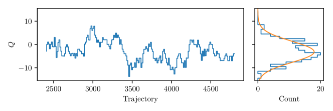
Figure 11: Topological charge history (left), and histogram (right), for the ensemble QB$\overline{5}$. Fitted parameters are $Q_{0}=-3.17(31)$, $\sigma=4.53(31)$, and $\tau_{\exp}=9.2(1)$.

Measurement	QB5FM2	QB$\bar{5}$FM2
$a\,m_{\rm PS}$	0.1850(4)	0.1848(3)
$a\,m_{\rm V}$	0.2680(15)	0.2722(17)
$a\,m_{\rm AV}$	0.449(7)	0.437(7)
$a\,m_{\rm S}$	0.428(6)	0.437(7)
$a\,m_{\rm T}$	0.2685(23)	0.2676(25)
$a\,m_{\rm AT}$	0.450(9)	0.448(9)
$a\,f_{\rm PS}$	0.03740(16)	0.03765(13)
$a\,f_{\rm V}$	0.0637(8)	0.0646(9)
$a\,f_{\rm AV}$	0.0749(27)	0.0682(21)

Table 7: Masses and (renormalised) decay constants, in lattice units, extracted from the measurements QB5FM2 and QB$\bar{5}$FM2. In parentheses are reported the statistical errors.

We measure, in the quenched approximation, the masses and (renormalised) decay constants for mesons built of fermions $Q$ transforming in the fundamental representation of $Sp(4)$. The results are shown in Table 7. We compare the measurements in QB5FM2 (used in the main analysis in the body of the paper) with the ones from the ensemble QB$\bar{5}$ with the same fermion mass (denoted QB$\bar{5}$FM2). The two sets of measurements are in agreement, within statistical errors, with all nine measurements within $1\sigma$ and $2\sigma$ of each other. Notice that systematic uncertainties are not included. In the body of the paper we did not include QB$\bar{5}$ in the analysis.

Appendix E Global symmetries and classification of mesons

Particle	Mass	$I^{G}J^{P{\cal C}}$	Hadronic
	(MeV)		decay mode(s)
$f_{0}(500)$	$500$	$0^{+}0^{++}$	$\pi\pi$
$f_{0}(980)$	$980$	$0^{+}0^{++}$	$\pi\pi$
$\eta$	$548$	$0^{+}0^{-+}$	$\pi\pi\pi$ ($\Delta{I}$)
$\eta^{\prime}$	$960$	$0^{+}0^{-+}$	$\eta\pi\pi$
$\omega$	$783$	$0^{-}1^{--}$	$\pi\pi\pi$
$\phi$	$1019$	$0^{-}1^{--}$	$\overline{K}K$
$f_{1}(1285)$	$1282$	$0^{+}1^{++}$	$4\pi,\eta\pi\pi$
$f_{1}(1420)$	$1426$	$0^{+}1^{++}$	$\overline{K^{\ast}}K,\overline{K}K\pi$
$h_{1}$	$1170$	$0^{-}1^{+-}$	$\rho\pi$
$h_{1}^{\prime}$	$1440$Abele:1997vu	$0^{-}1^{+-}$	$\overline{K^{\ast}}K$
$\omega(1420)$	1420	$0^{-}1^{--}$	$\rho\pi$
$\phi(1680)$	1680	$0^{-}1^{--}$	$\overline{K^{\ast}}K$
$\pi$	$135$	$1^{-}0^{-+}$	—
$a_{0}$	$980$	$1^{-}0^{++}$	$\eta\pi$
$\rho$	$775$	$1^{+}1^{--}$	$\pi\pi$
$a_{1}$	$1230$	$1^{-}1^{++}$	$\rho\pi,\pi\pi\pi$
$b_{1}$	$1230$	$1^{+}1^{+-}$	$\omega\pi$
$\rho(1450)$	$1465$	$1^{+}1^{--}$	$\pi\pi$

Table 8: Light mesons with $S=C=B=0$ in QCD Tanabashi:2018oca ; Abele:1997vu , their approximate masses, and quantum numbers. Charge conjugation ${\cal C}$ refers to the neutral component in multiplets including electrically charge particles, and $G\equiv{\cal C}(-1)^{I}$ for the whole multiplet. We show also representative hadronic decay modes. The three-body decay of $\eta$ violates isospin, and hence $G$-parity, and yields $\Gamma/M\sim 10^{-5}$.

In this Appendix, we review some symmetry properties of the mesons in more general gauge theories of relevance as candidates for the microscopic origin of CHMs. We discuss the cosets that control the long-distance behaviour of the theory at low temperatures and describe patterns of symmetry restoration and symmetry enhancement at high temperatures. We keep the discussion as general as possible but occasionally exemplify our observations with the specific case of the $Sp(4)$ gauge theory with $N_{f}=2$ and $n_{f}=3$.

Given a Lie group $G$ and its subgroup $H$, a generic element $\mathfrak{g}$ of the associated Lie algebra ${\cal G}$ can be decomposed as $\mathfrak{g}=\mathfrak{h}+\mathfrak{k}$, with $\mathfrak{h}\in{\cal H}$ an element of the algebra associated with $H$ and $\mathfrak{k}\in{\cal K}$ an element of the complement of ${\cal H}$ in ${\cal G}$. The coset space $G/H$ is said to be symmetric if, for all possible choices of $\mathfrak{h}$ and $\mathfrak{k}$, the following properties are true:

$$\left[\mathfrak{h}\,,\,\mathfrak{h}\right]\,\in\,{\cal H}\,,~{}~{}~{}~{}\left[\mathfrak{h}\,,\,\mathfrak{k}\right]\,\in\,{\cal K}\,,~{}~{}~{}~{}\left[\mathfrak{k}\,,\,\mathfrak{k}\right]\,\in\,{\cal H}\,.$$ (184)

These properties define in an unambiguous way an unbroken, multiplicative $\mathbb{Z}_{2}$ symmetry, which we can call $G$-parity, which is compatible with the Lie algebra, and upon which $\mathfrak{k}$ is assigned $G$-parity $-$, while $\mathfrak{h}$ is assigned $G$-parity $+$.

Three classes of cosets are commonly considered in the CHM context (see for instance Table I in Ref. Cacciapaglia:2019bqz ). They all emerge from gauge theories at the microscopic level.

• $SU(N_{f})_{L}\times SU(N_{f})_{R}/SU(N_{f})_{V}$ cosets are, for example, realised in $SU(N)$ gauge theories with $N_{f}$ fundamental Dirac fermions.

• $SU(2N_{f})/Sp(2N_{f})$ cosets are, for example, realised in $Sp(2N)$ gauge theories with $N_{f}$ fundamental Dirac fermions.

• $SU(2N_{f})/SO(2N_{f})$ cosets are, for example, realised in $Sp(2N)$ gauge theories with $N_{f}$ Dirac fermions transforming in the 2-index antisymmetric representation.

All these cosets are symmetric, and the resulting $G$-parity is a symmetry of the theories. It allows selection rules for scattering and decay processes to be established. We now discuss each of these possibilities in some detail, with emphasis on the properties of the mesons associated with the theories they emerge from.

We begin by reviewing the case of the $SU(3)$ gauge theory with $N_{f}=2$ light flavours. It describes the light mesons in QCD. The associated coset is $SU(2)_{L}\times SU(2)_{R}/SU(2)_{V}$. Much of what one learns from this theory is applicable to the other symmetric cosets listed above, with modifications that will be discussed later. In Table 8, we report some information about light QCD mesons with $S=C=B=0$, taken from the Particle Data Group Tanabashi:2018oca . We found Refs. Glozman:2007ek ; Glozman:2015qva ; Denissenya:2014ywa ; Rohrhofer:2017grg ; Glozman:2018jkb ; Rohrhofer:2019qwq ; Glozman:2019fku ; Engel:2011aa , and Appendix B in Ref. Gratrex:2018gmm particularly useful for the discussion that follows.

It is conventional to denote the states of QCD by the quantum numbers $I^{G}J^{P{\cal C}}$, where $I$ is the isospin (the representation of the unbroken $SU(2)_{V}$) and $J$ the spin. The assignment of $G$-parity for the isotriplets coincides with the traditional $G$-parity: it is related to charge-conjugation ${\cal C}$ of the neutral component in an isomultiplet, and the isospin $I$ of the isomultiplet, by the relation $G\equiv{\cal C}(-1)^{I}$, hence providing a link between the internal symmetry described above and a space-time symmetry. A second subtle link between internal and space-time symmetries involves the notion of spatial parity $P$; the $SU(2)_{L}$ and $SU(2)_{R}$ symmetries act, respectively, on the LH and RH projections of the spinors, while the unbroken subgroup is the (vectorial) symmetric combination of the two.

We start the discussion from the isotriplets $I=1$. The pions $\pi$ and axial vectors $a_{1}$ are, respectively, the lightest spin-0 and spin-1 states and are associated with the broken generators of the global symmetry, so that they have $G=-$; the vector mesons $\rho$ are associated with the unbroken group $SU(2)_{V}$, and have $G=+$. As a result, the $\rho$ decays to two $\pi$’s, while the $a_{1}$ decays to three $\pi$’s (or also one $\pi$ and one $\rho$). $G$-parity is a useful practical tool: while $\rho$ and $a_{1}$ particles both transform in the adjoint representation of the unbroken $SU(2)_{V}$ (isospin)—the unbroken subgroup and the coset have the same dimension—they are distinguished unambiguously by the different assignments of $G$, and hence they decay in different ways.

The global symmetries naturally extend to $U(2)_{L}\times U(2)_{R}/U(2)_{V}$. The additional unbroken vectorial $U(1)_{B}$ is the baryon number, and all mesons have vanishing $U(1)_{B}$ charge. The broken, anomalous, global, axial $U(1)_{A}$ symmetry plays an interesting role in relation to parity $P$. The axial $U(1)_{A}$ partners of the pions $\pi$, named $a_{0}$, have the same $G$-parity but opposite $P$. If the $U(1)_{A}$ were exact, $\pi$ and $a_{0}$ would be degenerate.

In the $J=1$, $I=1$ sector, the role played by the $U(1)_{A}$ symmetry is more subtle. The $\rho$ and $a_{1}$ mesons are sourced by bilinear operators V and AV, in which spinor indices are contracted on the $\gamma^{\mu}$ and $\gamma^{\mu}\gamma_{5}$ matrices, respectively. Such operators involve either two LH or two RH chiral spinors: the action of $U(1)_{A}$ leaves them both invariant, as they are two independent singlets of $U(1)_{A}$. But there is an important complication, as massive vectors in four dimensions can equivalently be described by 2-index antisymmetric tensors (see Appendix B and references therein). Two additional sources of spin-1 states T and AT are obtained by contracting the spinor indices on $\sigma^{\mu\nu}$ and $\sigma^{\mu\nu}\gamma_{5}$, respectively. The two operators T and AT couple the LH and RH chiral projections of the fermions, in a way that is similar to the $J=0$ isotriplet operators PS and S, that source the $\pi$ and $a_{0}$ particles. They form a doublet of the $U(1)_{A}\sim O(2)$ symmetry.

Because of symmetry breaking, the operator T (built with $\sigma^{\mu\nu}$) has the same quantum numbers $I^{G}J^{P{\cal C}}=1^{+}1^{--}$ as the source V (built from $\gamma^{\mu}$). The lightest and next-to-lightest states in this channel ($\rho$ and $\rho(1450)$ in Table 8) can approximately be thought of as resulting from the mixing of two states that have different $SU(2)_{L}\times SU(2)_{R}$ transformation properties and are sourced by different operators V and T. The $U(1)_{A}$ partner of the combination of $\rho$ and $\rho(1450)$ sourced by T is denoted by $b_{1}$ (see again Table 8), and sourced by AT.

Because we are also comparing with real-world QCD, we should notice that the isosinglet $I=0$ sector is complicated by the fact that real-world light mesons are better explained by a model in which one includes $2+1$ quarks, including the heavier strange quark $s$. The isosinglet mesons include an additional tower of states, due to mixing with the $(\bar{s}s)$ singlet. In Table 8, this results in the doubling of states with $I=0$ in respect to the $I=1$ case, as we chose to retain pairs of mesons with identical quantum numbers. The $G$-parity assignment of each isosinglet state is the opposite of that of the corresponding isotriplet with the same $J^{P{\cal C}}$. Notice in the table that the decay of the $\eta$ to $3\pi$ violates $G$-parity: it yields a suppressed rate $\Gamma$, with $\Gamma/M\sim 10^{-5}$, and originates from explicit breaking of isospin in real-world QCD, in which, for instance, up and down quarks are not degenerate in mass.

The $I=0$ and $J=0$ lightest states are the $f_{0}(500)/f_{0}(980)$ and their $U(1)_{A}$ partners, the $\eta/\eta^{\prime}$ pair. The $I=0$ and $J=1$ sector contains the pairs $\omega/\phi$, $f_{1}(1285)/f_{1}(1420)$, $h_{1}/h_{1}^{\prime}$, and $\omega(1420)/\phi(1680)$. The four of them play the same roles as, respectively, the $\rho$, $a_{1}$, $b_{1}$, and $\rho(1450)$ mesons, in the isotriplet case. One linear combination of the two $\omega/\phi$ pairs is sourced by the bilinear operator T, which forms a doublet of $U(1)_{A}$ with the source AT of the $h_{1}/h_{1}^{\prime}$ pair.

Let us see how these considerations have to be modified for enlarged cosets. (Both the $SU(2N_{f})/Sp(2N_{f})$ and $SU(2N_{f})/SO(2N_{f})$ contain the $SU(N_{f})_{L}\times SU(N_{f})_{R}/SU(N_{f})_{V}$ subspace, enhanced because of the (pseudo)real nature of the underlying fermion representations.) The unbroken baryon number $U(1)_{B}$ is a subset of the unbroken part of these two cosets rather than commuting with it. Diquark operators hence source mesons, that complete the representation of $SU(N_{f})_{V}$ into full representations of the unbroken $Sp(2N_{f})$ or $SO(2N_{f})$. The unbroken group and the coset have in these cases different dimension, so that representations with different $G$-parity have different dimensionality as well (see Table 4 for instance), rendering $G$-parity redundant, at least as a way to distinguish among them.

We conclude by discussing explicitly the general form of the operators to be used as sources. We start from a two-component spinor $\chi$ transforming in the fundamental representation of the global $SU(2N_{f})$ symmetry group. A spin-0 local operator $J^{0}$ takes the schematic form $\chi^{\mathrm{T}}\tilde{C}\chi$. The product of two fundamental decomposes as

$$2N_{f}\otimes 2N_{f}=\left[N_{f}(2N_{f}-1)\right]\oplus\left[N_{f}(2N_{f}+1)\right]\,,$$ (185)

into the 2-index antisymmetric and symmetric representations of $SU(2N_{f})$, respectively. Furthermore, depending on whether the unbroken subgroup is $Sp(2N_{f})$ or $SO(2N_{f})$, either the antisymmetric or the symmetric combination is reducible and further decomposes into the unbroken subgroup by projecting one element along the elementary symplectic matrix $\Omega$ or the symmetric $\omega$, respectively. Excitations sourced by this operator correspond to the $f_{0}$ of QCD-like theories, while those along the complement correspond to the PS flavoured states (the $\pi$ of QCD). The representation that is irreducible, instead, would coincide with the adjoint of the unbroken subgroup, except that it vanishes because of Fermi statistics—unless one considers nonlocal operators.

Along the same lines, the spin-1 local operator $J^{1}$ schematically reads ${\chi}^{\dagger}\bar{\sigma}^{\mu}\chi$, and the decomposition in $SU(2N_{f})$ takes the form

$$\overline{2N_{f}}\otimes 2N_{f}=1\oplus\left[4N_{f}^{2}-1\right]\,.$$ (186)

After decomposition into the representations of the unbroken subgroup, the adjoint splits into its antisymmetric and symmetric parts, and hence one ultimately finds the same decomposition as in the spin-0 case. This property descends from the (pseudo)real nature of $Sp(2N_{f})$ and $SO(2N_{f})$, that do not distinguish the fundamental representation $2N_{f}$ from its conjugate. It is useful to notice that the four operators V, T, AV, and AT states source only one state that is a singlet. This is different from the $SU(N_{f})_{L}\times SU(N_{f})_{R}/SU(N_{f})_{V}$, where each of the four operators sources a singlet of the unbroken group: the three additional $J=1$ states are part of the irreducible representations sourced by V, T, and AT.

Summarising for the $SU(2N_{f})/Sp(2N_{f})$ and $SU(2N_{f})/SO(2N_{f})$ cases: pseudoscalar PS and axial-vector AV multiplets have the same degeneracies, as do the flavoured scalar S—the $U(1)_{A}$ partners of the PS states. The vector states V belong to a different representation of the unbroken group common also to the antisymmetric tensor T, as well as to its $U(1)_{A}$ partner AT. In the unbroken $Sp(2N_{f})$ case, the V, T and AT mesons span a complete symmetric representation of $Sp(2N_{f})$, with PS, S, and AV on the (antisymmetric) complement. The reverse is true in the case of $SO(2N_{f})$ (see again Table 4). In both cases, the singlet sector is simpler: it consists of two spin-0 states forming a $U(1)_{A}$ doublet and of one isolated spin-1 singlet state.

E.1 Symmetry restoration and enhancement

At high temperatures, the fermion condensates melt, leading to restoration of the global symmetries. Both the non-Abelian $SU(2N_{f})$ (or $SU(N_{f})\times SU(N_{f})$) global symmetry, as well as the Abelian $U(1)_{A}$ symmetry are restored Pisarski:1983ms (see also Chiu:2013wwa ; Brandt:2019ksy ; Suzuki:2019vzy for progress on $N_{f}=2$ lattice QCD). As a consequence of the former, one might find that the states sourced by V and AV operators become degenerate (the $\rho$ and $a_{1}$ in the QCD-like case). Because of the latter, $U(1)_{A}$ multiplets should become degenerate, for example the states sourced by PS and S operators (the $\pi$ and $a_{0}$ mesons in the QCD-like case). See for instance Ref. Lee:2017uvl and references therein.

Recent studies have emerged suggesting that, because the thermal bath reduces the space-time symmetries, the global internal symmetry is further enhanced, with the emergence of a new chiral-spin symmetry that combines with the global symmetries. We refer the reader to Refs. Glozman:2007ek ; Glozman:2015qva ; Denissenya:2014ywa ; Rohrhofer:2017grg ; Glozman:2018jkb ; Rohrhofer:2019qwq ; Glozman:2019fku for this research field, in which the specific case of the QCD-like, $SU(3)$ theory with $N_{f}=2$ is discussed in great detail, and numerical evidence of the emergence of a $SU(4)$ global symmetry is exposed, in the channels with spin $J>0$. In the following, we limit ourselves to producing a summary of what would be the (testable) expectations in the three main cosets of interest to CHMs, if the corresponding symmetry-restoration and symmetry-enhancement patterns were to be confirmed.

• The $SU(N_{f})_{L}\times SU(N_{f})_{R}/SU(N_{f})_{V}$ cosets can emerge, at $T=0$, from theories with complex representations, for example the $SU(N)$ gauge theories with $N_{f}$ fundamental Dirac fermions. These cosets are accompanied by the anomalous $U(1)_{A}=U(1)_{L}\times U(1)_{R}/U(1)_{B}$ Abelian coset. At high temperatures, the global $U(N_{f})_{L}\times U(N_{f})_{R}$ symmetry is restored and enhanced to $U(2N_{f})=U(1)_{A}\times SU(2N_{f})$. For example, in the $N_{f}=2$ case that approximates QCD, in the $J=1$ sector, four of the $I=1$ states (the two lightest $\rho$, the $a_{1}$, and the $b_{1}$) and four of the $I=0$ states (the two $\omega/\phi$, the $f_{1}/f_{1}^{\prime}$, and the $h_{1}/h_{1}^{\prime}$) have been measured to become degenerate, which would be compatible with forming a complete $16$-dimensional adjoint representation of the $U(1)\times SU(4)$ enhanced global symmetry group Glozman:2007ek ; Glozman:2015qva ; Denissenya:2014ywa ; Rohrhofer:2017grg ; Glozman:2018jkb ; Rohrhofer:2019qwq ; Glozman:2019fku ; Engel:2011aa . In the $J=0$ sector, this symmetry is not manifest: the $\pi$ and $a_{0}$ combine with the $f_{0}/f_{0}^{\prime}$ and the $\eta/\eta^{\prime}$ to form $2N_{f}^{2}$ degenerate states, the adjoint of the symmetry group $U(N_{f})_{L}\times U(N_{f})_{R}$. (It would require an additional $2N_{f}^{2}$ components, two copies of the adjoint of $U(N_{f})$, to complete the adjoint of $U(2N_{f})$.)

• The $SU(2N_{f})/Sp(2N_{f})$ cosets can emerge, at $T=0$, from theories with pseudoreal representations, for example the $Sp(2N)$ gauge theories with $N_{f}$ Dirac fundamental fermions. In addition, the anomalous $U(1)_{A}$ is also spontaneously broken. What would have been the unbroken $U(1)_{B}$ associated with the baryon number in the case of complex representations is now a subgroup of the nonanomalous $Sp(2N_{f})$. Going to a high temperature, the symmetry is expected to be first restored and then enhanced to $Sp(4N_{f})$. For example, in the $N_{f}=2$ case, in the $J=1$ sector of the spectrum, the ten V and ten T mesons (which include both the correspondent of the $\rho$ and $\omega/\phi$ of QCD), the five AV mesons (corresponding to the $a_{1}$), the ten AT mesons (which include both states corresponding to the $b_{1}$ and $h_{1}/h_{1}^{\prime}$ of QCD) and the singlet vector state (corresponding to the $f_{1}/f_{1}^{\prime}$) form a complete, $36$-dimensional adjoint representation of $Sp(8)$. The $J=0$ sector is not expected to show high-$T$ symmetry enhancement. PS flavoured states combine with the singlet to form the antisymmetric representation (in the QCD analogy, they correspond to the $\pi$ and the $f_{0}/f_{0}^{\prime}$), and their $U(1)_{A}$ partners (the $a_{0}$ and the $\eta/\eta^{\prime}$ in QCD) combine to form the complex, antisymmetric 2-index representation of $SU(2N_{f})$, which has dimension $2\times N_{f}(2N_{f}-1)$. (It would require finding an adjoint representation of $SU(2N_{f})$ of dimension $4N_{f}^{2}-1$, to yield a total of $8N_{f}^{2}-2N_{f}-1$, which is the 2-index antisymmetric of $Sp(4N_{f})$. In the $N_{f}=2$ case, the antisymmetric of $Sp(8)$ decomposes as $27=15+6_{\mathbb{C}}$ in terms of $SU(4)$, and the $15$ is missing.)

• The $SU(2n_{f})/SO(2n_{f})$ cosets can emerge, at $T=0$, from theories with real representations, for example the $Sp(2N)$ gauge theories with $n_{f}$ Dirac fermions transforming as the 2-index antisymmetric representation. At high temperatures, the restoration of the symmetry is expected to be followed by its enhancement to a global $SO(4n_{f})$. For example, if $n_{f}=3$, in the spin-1 flavoured sector the $15$ v, $15$ t and $15$ at mesons sourced by the operators in Table 4 will be degenerate with the $20^{\prime}$ av mesons. In addition, a flavour-singlet vector will also be degenerate, and together will yield the $66$-dimensional antisymmetric (adjoint) representation of $SO(12)$, with spin $J=1$. In the spin $J=0$ sector, the $20^{\prime}$ ps and $20^{\prime}$ s mesons, together with the $1+1$ flavor singlets form the $21_{\mathbb{C}}$ representation of $SU(6)$. (It would require an additional $35$, the adjoint of $SU(6)$, to make the 2-index symmetric traceless $77$-dimensional representation of $SO(12)$.)

Appendix F Bilinear operators as sources

We collect in this Appendix technical clarifications about gauge-invariant operators ${\cal O}_{M}$, written in terms of the four-component fermions $Q$ and $\Psi$, to be used as sources in the lattice calculations of the spectrum of composite states. We consider the $Sp(2N)$ gauge theory, without specifying $N$. When possible, we also write our expression in a form that applies to $Sp(2N_{f})$ and $SO(2n_{f})$ groups with general $N_{f}$ fundamental and $n_{f}$ antisymmetric Dirac fermions. For concreteness, in Appendix F.1 we explicitly identify the irreducible representations of the unbroken global $Sp(4)$ group of relevance in the context of CHMs, as well as their $SU(2)_{L}\times SU(2)_{R}$ decompositions.

In the case of $N_{f}$ Dirac spinors transforming in the fundamental representation of the gauge group $Sp(2N)$, the fermion bilinear operators are written as in terms of $N_{f}\times N_{f}$ block matrices, built from the $N_{f}$ Dirac fermions

$$Q^{i\,a}=\left(\begin{array}[]{c}q^{i\,a}\cr-\Omega^{ab}(\tilde{C}q^{N_{f}+i\,{\ast}})_{b}\end{array}\right)\,,$$ (189)

and, following the same lines leading to Eqs. (112), their conjugate Dirac fermion as

$$Q^{i\,a}_{C}\equiv-\gamma_{5}\Omega^{ab}C(\overline{Q^{i}}^{\mathrm{T}})_{b}=-\gamma_{5}\Omega^{ab}C\gamma^{0}(Q^{i\ast})_{b}=\left(\begin{array}[]{c}q^{N_{f}+i\,a}\cr-\Omega^{ab}(\tilde{C}q^{i\,{\ast}})_{b}\end{array}\right)\,.$$ (192)

Notice a difference, with respect to the definition leading to Eq. (112), in how we define the conjugate spinor: the factor of $-\gamma_{5}\Omega^{ab}$ is introduced, in order to make the decomposition in LH and RH chiral components of $Q$ and $Q_{C}$ take the same form. We stress that $Q_{C}^{i}$ is physically equivalent to $Q^{i}$, and hence one can identify the $N_{f}$ Dirac fermions with $Q^{i}$.

We write explicitly the form of the general $2N_{f}\times 2N_{f}$ matrices built as bilinears in spinors, both in two-component and four-component notation, which read

$$J_{0} = \left(\begin{array}[]{c|c}\cr\overline{Q^{i\,a}_{C}}P_{L}Q^{j\,a}&\overline{Q^{i\,a}_{C}}P_{L}Q^{j\,a}_{C}\cr\cr\hline\cr\cr\overline{Q^{i\,a}}P_{L}Q^{j\,a}&\overline{Q^{i\,a}}P_{L}Q^{j\,a}_{\,C}\cr\end{array}\right)=\Omega_{ab}\left(\begin{array}[]{c|c}\cr q^{i\,a\,\mathrm{T}}\tilde{C}q^{j\,b}&q^{i\,a\,\mathrm{T}}\tilde{C}q^{N_{f}+j\,b}\cr\cr\hline\cr\cr q^{N_{f}+i\,a\,\mathrm{T}}\tilde{C}q^{j\,b}&q^{N_{f}+i\,a\,\mathrm{T}}\tilde{C}q^{N_{f}+j\,b}\cr\end{array}\right),$$ (203)

$$J_{1}^{\mu} = \left(\begin{array}[]{c|c}\cr\overline{Q^{i\,a}}\gamma^{\mu}P_{L}Q^{j\,a}&\overline{Q^{i\,a}}\gamma^{\mu}P_{L}Q^{j\,a}_{C}\cr\cr\hline\cr\cr\overline{Q^{i\,a}_{C}}\gamma^{\mu}P_{L}Q^{j\,a}&\overline{Q^{i\,a}_{C}}\gamma^{\mu}P_{L}Q^{j\,a}_{\,C}\cr\end{array}\right)=\left(\begin{array}[]{c|c}\cr q^{i\,a\,\dagger}\bar{\sigma}^{\mu}q^{j\,a}&q^{i\,a\,\dagger}\bar{\sigma}^{\mu}q^{N_{f}+j\,a}\cr\cr\hline\cr\cr q^{N_{f}+i\,a\,\dagger}\bar{\sigma}^{\mu}q^{j\,a}&q^{N_{f}+i\,a\,\dagger}\bar{\sigma}^{\mu}q^{N_{f}+j\,a}\cr\end{array}\right),$$ (214)

and

$$J_{1^{\prime}}^{\mu\nu}=\left(\begin{array}[]{c|c}\cr\overline{Q^{i\,a}_{C}}\sigma^{\mu\nu}P_{L}Q^{j\,a}&\overline{Q^{i\,a}_{C}}\sigma^{\mu\nu}P_{L}Q^{j\,a}_{C}\cr\cr\hline\cr\cr\overline{Q^{i\,a}}\sigma^{\mu\nu}P_{L}Q^{j\,a}&\overline{Q^{i\,a}}\sigma^{\mu\nu}P_{L}Q^{j\,a}_{\,C}\cr\end{array}\right)\,=\Omega_{ab}\left(\begin{array}[]{c|c}\cr q^{i\,a\,\mathrm{T}}\tilde{C}\sigma^{\mu\nu}_{LL}q^{j\,b}&q^{i\,a\,\mathrm{T}}\tilde{C}\sigma^{\mu\nu}_{LL}q^{N_{f}+j\,b}\cr\cr\hline\cr\cr q^{N_{f}+i\,a\,\mathrm{T}}\tilde{C}\sigma^{\mu\nu}_{LL}q^{j\,b}&q^{N_{f}+i\,a\,\mathrm{T}}\tilde{C}\sigma^{\mu\nu}_{LL}q^{N_{f}+j\,b}\cr\end{array}\right)\,.$$ (225)

The symplectic matrix $\Omega_{2N_{f}}$ is defined as a $2N_{f}\times 2N_{f}$ antisymmetric matrix such that $(\Omega_{2N_{f}})^{2}=-\mathbb{1}_{2N_{f}}$. Because of the contraction with $\Omega_{ab}$, $J_{0}$ is antisymmetric. This bilinear condenses, and hence the unbroken subgroup is $Sp(2N_{f})$. The decomposition of $J_{0}$, $J_{1}^{\mu}$ and $J_{1^{\prime}}^{\mu\nu}$ in their irreducible representations is $2N_{f}\otimes 2N_{f}=\left[N_{f}(2N_{f}-1)-1\right]\oplus 1\oplus N_{f}(2N_{f}+1)$:

$$J_{0,1,1^{\prime}} = \left[\frac{1}{2}\left(J_{0,1,1^{\prime}}-(J_{0,1,1^{\prime}})^{\mathrm{T}}\right)+\frac{\Omega_{2N_{f}}}{2N_{f}}{\rm Tr\,}\left\{\Omega_{2N_{f}}J_{0,1,1^{\prime}}\right\}\right]-\frac{\Omega_{2N_{f}}}{2N_{f}}{\rm Tr\,}\left\{\Omega_{2N_{f}}J_{0,1,1^{\prime}}\right\}\,+\,$$ (226)

$$\,+\,\frac{1}{2}\left(J_{0,1,1^{\prime}}+(J_{0,1,1^{\prime}})^{\mathrm{T}}\right)\,\equiv\,J_{0,1,1^{\prime}}^{(A)}\,+J_{0,1,1^{\prime}}^{(1)}\,+\,J_{1,1^{\prime}}^{(S)}\,.$$

We highlighted here the fact that the symmetric part of $J_{0}$ vanishes identically. Notice also that the singlets are antisymmetric. Both the $J_{1}$ and $J_{1^{\prime}}$ decompose into symmetric and antisymmetric parts, the latter expected to be related to heavier states. For the $SU(2N_{f})/Sp(2N_{f})$ coset the operators in Table 4 are identified as follows:

$${\cal O}_{\rm PS}=J_{0}^{(A)}\,,~{}~{}~{}{\cal O}_{\rm V}=J_{1}^{(S)}\,,~{}~{}~{}{\cal O}_{\rm AV}=J_{1}^{(A)}\,,~{}~{}~{}{\cal O}_{\rm T}=J_{1^{\prime}}^{(S)}\,,$$ (227)

with the ${\cal O}_{\rm S}$ and ${\cal O}_{\rm AT}$ operators being the $U(1)_{A}$ conjugates of ${\cal O}_{\rm PS}$ and ${\cal O}_{\rm T}$, respectively.

With matter content including $n_{f}$ Dirac fermions in the antisymmetric representation of $Sp(2N)$ (for $N>1$) we introduce the analogous $j_{0,1,1^{\prime}}$ operators built from the fermions

$$\Psi^{i\,ab}=\left(\begin{array}[]{c}\psi^{i\,ab}\cr-\Omega^{ac}\Omega^{bd}(\tilde{C}\psi^{n_{f}+i\,^{\ast}})_{cd}\end{array}\right)\,,$$ (230)

with $i=1\,,\,\cdots\,,\,n_{f}$, together with their conjugates

$$\Psi^{i\,ab}_{C}\equiv\Omega^{ac}\Omega^{bd}C(\overline{\Psi^{i}}^{\mathrm{T}})_{\,\,cd}\equiv\Omega^{ac}\Omega^{bd}C\gamma^{0}(\Psi^{i\ast})_{cd} = \left(\begin{array}[]{c}\psi^{n_{f}+i\,ab}\cr-\Omega^{ac}\Omega^{bd}(\tilde{C}\psi^{i\,^{\ast}})_{cd}\end{array}\right)\,.$$ (233)

We conventionally align the vacuum with the matrix $\omega_{2n_{f}}$, the $2n_{f}\times 2n_{f}$ symmetric matrix such that $(\omega_{2n_{f}})^{2}=\mathbb{1}_{2n_{f}}$, generalising Eq. (15). We decompose $j_{0,1,1^{\prime}}$ in irreducible representations as $2n_{f}\otimes 2n_{f}=\left[n_{f}(2n_{f}+1)-1\right]\oplus 1\oplus n_{f}(2n_{f}-1)$:

$$j_{0,1,1^{\prime}} = \left[\frac{1}{2}\left(j_{0,1,1^{\prime}}+(j_{0,1,1^{\prime}})^{\mathrm{T}}\right)-\frac{\omega_{2n_{f}}}{2n_{f}}{\rm Tr\,}\left\{\omega_{2n_{f}}j_{0,1,1^{\prime}}\right\}\right]+\frac{\omega_{2n_{f}}}{2n_{j}}{\rm Tr\,}\left\{\omega_{2n_{f}}j_{0,1,1^{\prime}}\right\}\,+\,$$ (234)

$$\,+\,\frac{1}{2}\left(j_{0,1,1^{\prime}}-(j_{0,1,1^{\prime}})^{\mathrm{T}}\right)\,\equiv\,j_{0,1,1^{\prime}}^{(S)}\,+j_{0,1,1^{\prime}}^{(1)}\,+\,j_{1,1^{\prime}}^{(A)}\,.$$

We highlighted the fact that the antisymmetric part of $j_{0}$ vanishes. In this case, the singlets are symmetric matrices.

We write these operators in $n_{f}\times n_{f}$ blocks as matrix representations of the global $SU(2n_{f})$ symmetry:

$$j_{0} = \left(\begin{array}[]{c|c}\cr\overline{\Psi^{i\,ab}_{C}}P_{L}\Psi^{j\,ab}&\overline{\Psi^{i\,ab}_{C}}P_{L}\Psi^{j\,ab}_{C}\cr\cr\hline\cr\cr\overline{\Psi^{i\,ab}}P_{L}\Psi^{j\,ab}&\overline{\Psi^{i\,ab}}P_{L}\Psi^{j\,ab}_{\,C}\cr\end{array}\right)\,=\Omega_{ac}\Omega_{bd}\left(\begin{array}[]{c|c}\cr\psi^{i\,ab\,\mathrm{T}}\tilde{C}\psi^{j\,cd}&\psi^{i\,ab\,\mathrm{T}}\tilde{C}\psi^{n_{f}+j\,cd}\cr\cr\hline\cr\cr\psi^{n_{f}+i\,ab\,\mathrm{T}}\tilde{C}\psi^{j\,cd}&\psi^{n_{f}+i\,ab\,\mathrm{T}}\tilde{C}\psi^{n_{f}+j\,cd}\cr\end{array}\right)\,,$$ (245)

$$j_{1}^{\mu} = \left(\begin{array}[]{c|c}\cr\overline{\Psi^{i\,ab}}\gamma^{\mu}P_{L}\Psi^{j\,ab}&\overline{\Psi^{i\,ab}}\gamma^{\mu}P_{L}\Psi^{j\,ab}_{C}\cr\cr\hline\cr\cr\overline{\Psi^{i\,ab}_{C}}\gamma^{\mu}P_{L}\Psi^{j\,ab}&\overline{\Psi^{i\,ab}_{C}}\gamma^{\mu}P_{L}\Psi^{j\,ab}_{\,C})\cr\end{array}\right)\,=\left(\begin{array}[]{c|c}\cr\psi^{i\,ab\,\dagger}\bar{\sigma}^{\mu}\psi^{j\,ab}&\psi^{i\,ab\,\dagger}\bar{\sigma}^{\mu}\psi^{n_{f}+j\,ab}\cr\cr\hline\cr\cr\psi^{n_{f}+i\,ab\,\dagger}\bar{\sigma}^{\mu}\psi^{j\,ab}&\psi^{n_{f}+i\,ab\,\dagger}\bar{\sigma}^{\mu}\psi^{n_{f}+j\,ab}\cr\end{array}\right)\,,$$ (256)

and

$$j_{1^{\prime}}^{\mu\nu}=\left(\begin{array}[]{c|c}\cr\overline{\Psi^{i\,ab}_{C}}\sigma^{\mu\nu}P_{L}\Psi^{j\,ab}&\overline{\Psi^{i\,ab}_{C}}\sigma^{\mu\nu}P_{L}\Psi^{j\,ab}_{C}\cr\cr\hline\cr\cr\overline{\Psi^{i\,ab}}\sigma^{\mu\nu}P_{L}\Psi^{j\,ab}&\overline{\Psi^{i\,ab}}\sigma^{\mu\nu}P_{L}\Psi^{j\,ab}_{\,C}\cr\end{array}\right)\,=\Omega_{ac}\Omega_{bd}\ \left(\begin{array}[]{c|c}\cr\psi^{i\,ab\,\mathrm{T}}\tilde{C}\sigma^{\mu\nu}_{LL}\psi^{j\,cd}&\psi^{i\,ab\,\mathrm{T}}\tilde{C}\sigma^{\mu\nu}_{LL}\psi^{n_{f}+j\,cd}\cr\cr\hline\cr\cr\psi^{n_{f}+i\,ab\,\mathrm{T}}\tilde{C}\sigma^{\mu\nu}_{LL}\psi^{j\,cd}&\psi^{n_{f}+i\,ab\,\mathrm{T}}\tilde{C}\sigma^{\mu\nu}_{LL}\psi^{n_{f}+j\,cd}\cr\end{array}\right)\,.$$ (267)

In the $SU(2n_{f})/SO(2n_{f})$ case, the operators in Table 4 are identified as follows:

$${\cal O}_{\rm ps}=j_{0}^{(S)}\,,~{}~{}~{}{\cal O}_{\rm v}=j_{1}^{(A)}\,,~{}~{}~{}{\cal O}_{\rm av}=j_{1}^{(S)}\,,~{}~{}~{}{\cal O}_{\rm t}=j_{1^{\prime}}^{(A)}\,.$$ (268)

Again, ${\cal O}_{\rm s}$ and ${\cal O}_{\rm at}$ operators are the $U(1)_{A}$ conjugates of ${\cal O}_{\rm ps}$ and ${\cal O}_{\rm t}$, respectively.

As explained also in Appendix E, operators $J_{0}$ that source spin-0 states, and operators $J_{1}$ sourcing spin-1 states can be classified in terms of the original global $SU(2N_{f})$ (enlarged) symmetry, according to which the former transform as $2N_{f}\otimes 2N_{f}=\left[N_{f}(2N_{f}-1)\right]\oplus\left[N_{f}(2N_{f}+1)\right]$, and the latter as $\overline{2N_{f}}\otimes 2N_{f}=1\oplus\left[4N_{f}^{2}-1\right]$ of $SU(2N_{f})$. Only once the $SU(2N_{f})$ is broken to its $Sp(2N_{f})$ group, $J_{0}$ and $J_{1}$ decompose in the same set of irreducible representations of the subgroup. Similarly, operators $J_{1^{\prime}}$ couple LH to RH components of the Dirac fields, and hence while they source particles with the same spin as $J_{1}$, they transform under $SU(2N_{f})$ in the same way as $J_{0}$. Once the symmetry is broken, mixing between the particles sourced by $J_{1}$ and $J_{1^{\prime}}$ will ensue, but in general these are different sources for different $SU(2N_{f})$ particles. The same considerations apply to the $j_{0,1,1^{\prime}}$ operators, and their decompositions in irreducible representations of the $SO(2n_{f})$ subgroup.

One can now explicitly decompose the matrices $J_{0,1,1^{\prime}}$ (and $j_{0,1,1^{\prime}}$) into a given basis of the $U(N_{f})$ (and $U(n_{f})$), by making a choice of generators $T^{A}$ (and $t^{B}$) of the group. We devote the next subsection to showing the result of this process in the $SU(4)/Sp(4)$ case, for some of the interesting operators.

F.1 $SU(4)/Sp(4)$ composite operators

We focus on the $Sp(2N)$ theory with $N_{f}=2$ fundamental fermions, and its $SU(4)/Sp(4)$ coset, which is relevant in the CHM context (see also the discussion in Drach:2017btk ).

The pions in Eq. (171) are sourced by the antisymmetric ${\cal O}_{\rm PS}=J_{0}^{(A)}$ operators. We can add to the Lagrangian density in Eq. (II.3) the following source term:

$${\cal L}_{\pi} = \frac{\sqrt{2}f}{2}{\rm Tr\,}\left[J_{0}\Sigma^{\ast}+{\rm h.c.}\right]\,,$$ (269)

where $\Sigma=e^{\frac{2i\pi}{f}}\Omega$ is the antisymmetric matrix defined in Eq. (26). We can expand for small $\pi/f$ and make use of the antisymmetry in flavour space of $J_{0}$. We make explicit use of the generators as written in Eq. (B.4) of Ref. Lee:2017uvl . Looking at the decomposition of the $5$ according to $SO(4)\sim SU(2)_{L}\times SU(2)_{R}\subset Sp(4)$, we find that the $SO(4)$-singlet $\pi^{3}$ is sourced by the operator ${\cal O}_{{\rm PS},3}\equiv\,i\,{\delta{\cal L}_{\pi}}/{\delta\pi^{3}}$ that reads

$${\cal O}_{{\rm PS},3} = \frac{i}{2}\left(\frac{}{}iJ_{0}^{13}-iJ_{0}^{31}-iJ_{0}^{24}+iJ_{0}^{42}\,+\,{\rm c.c.}\frac{}{}\right)=\left(\overline{Q^{1\,a}}\gamma^{5}Q^{1\,a}-\overline{Q^{2\,a}}\gamma^{5}Q^{2\,a}\right),$$ (270)

where we made abundant use of Eqs. (113). The $4$ of $SO(4)$ are sourced by the following operators ${\cal O}_{{\rm PS},A}\,\equiv\,i\,{\delta{\cal L}_{\pi}}/{\delta\pi^{A}}$ given by

$${\cal O}_{{\rm PS},1} = \frac{i}{2}\left(\frac{}{}+iJ_{0}^{14}-iJ_{0}^{41}+iJ_{0}^{23}-iJ_{0}^{32}\,+\,{\rm c.c.}\frac{}{}\right)=\left(\overline{Q^{1\,a}}\gamma^{5}Q^{2\,a}+\overline{Q^{2\,a}}\gamma^{5}Q^{1\,a}\right)\,,$$

$${\cal O}_{{\rm PS},2} = \frac{i}{2}\left(\frac{}{}-J_{0}^{14}+J_{0}^{41}+J_{0}^{23}-J_{0}^{32}\,+\,{\rm c.c.}\frac{}{}\right)=\left(-i\overline{Q^{1\,a}}\gamma^{5}Q^{2\,a}+i\,\overline{Q^{2\,a}}\gamma^{5}Q^{1\,a}\right)\,,$$

$${\cal O}_{{\rm PS},4} = \frac{i}{2}\left(\frac{}{}+J_{0}^{12}-J_{0}^{21}-J_{0}^{34}+J_{0}^{43}\,+\,{\rm c.c.}\frac{}{}\right)=-i\,\left(\overline{Q^{1\,a}}Q^{2\,a}_{\,C}+\overline{Q_{C}^{2\,a}}Q^{1\,a}\right)\,,$$ (271)

$${\cal O}_{{\rm PS},5} = \frac{i}{2}\left(\frac{}{}-iJ_{0}^{12}+iJ_{0}^{21}-iJ_{0}^{34}+iJ_{0}^{43}\,+\,{\rm c.c.}\frac{}{}\right)=i\,\left(-i\,\overline{Q^{1\,a}}Q^{2\,a}_{C}+i\overline{Q^{2\,a}_{C}}Q^{1\,a}\right)\,.$$

The additional operator given by

$${\cal O}_{{\rm PS},0} \equiv -\frac{1}{2}\left(\frac{}{}J_{0}^{13}+J_{0}^{24}-J_{0}^{31}-J_{0}^{42}+{\rm c.c}\frac{}{}\right)\,=\,\left(\overline{Q^{1\,a}}Q^{1\,a}+\overline{Q^{2\,a}}Q^{2\,a}\right)$$ (272)

is aligned along $\Omega$, in the internal space. It is the operator that develops a nontrivial VEV. It sources the $Sp(4)$ singlet, which has the same role as the $f_{0}(500)$ of QCD (see Table 8). Notice that these $6$ operators put together transform as the antisymmetric representation of the global $SU(4)$, before the decomposition in $Sp(4)$ irreducible representations as $6=1+5$.

Six additional operators ${\cal O}_{{\rm S},i}$ can be obtained by replacing $\mathbb{1}_{4}\rightarrow i\gamma^{5}$ from the operators ${\cal O}_{{\rm PS},i}$ for $i=0\,,\,\cdots\,,\,5$. Such operators are related to the former by the (anomalous) global $U(1)_{A}\sim O(2)$ symmetry. (In QCD, the $U(1)_{A}$ partners of the $\pi$ and $f_{0}(500)$ particles are, respectively, the $a_{0}$ and $\eta/\eta^{\prime}$ particles.)

The sources of the spin-1 fields are given in terms of the operators in $J_{1}^{\mu}$. In Sec. II.3 we introduced the fields $A_{\mu}=\sum_{A=1}^{15}A^{A}_{\,\,\mu}T^{i}$ (we drop here the subscript $6$), with $T^{A}$ the Hermitian generators of $SU(4)$ normalised as ${\rm Tr\,}T^{A}T^{B}=\frac{1}{2}\delta^{AB}$. As in Ref. Lee:2017uvl , it is convenient to label the broken generators with $A=1\,,\,\cdots\,,\,5$, and the unbroken ones with $A=6\,,\,\cdots\,,\,15$. We hence add to the Lagrangian density the following source term:

$${\cal L}_{A} = \sqrt{2}{\rm Tr\,}\left[J_{1}^{\mu}A_{\mu}^{\mathrm{T}}\right]+{\rm h.c.}\,.$$ (273)

Starting from the AV sources, we find that ${\cal O}_{{\rm AV},A}^{\,\,\mu}\,\equiv\,\frac{\delta{\cal L}_{A}}{\delta A^{A}_{\,\,\mu}}$ are given by the following

$$\,{\cal O}_{{\rm AV},1}^{\,\,\mu}\, = \frac{1}{2}\left(\frac{}{}\,J_{1}^{12}+\,J_{1}^{21}+\,J_{1}^{34}+\,J_{1}^{43}\,+\,{\rm c.c.}\right)=\overline{Q^{1\,a}}\gamma^{\mu}\gamma^{5}Q^{2\,a}+\,\overline{Q^{2\,a}}\gamma^{\mu}\gamma^{5}Q^{1\,a}\,,$$

$$\,{\cal O}_{{\rm AV},2}^{\,\,\mu} = \frac{1}{2}\left(\frac{}{}\,-iJ_{1}^{12}+i\,J_{1}^{21}+i\,J_{1}^{34}-i\,J_{1}^{43}\,+\,{\rm c.c.}\right)=-i\,\overline{Q^{1\,a}}\gamma^{\mu}\gamma^{5}Q^{2\,a}+i\,\overline{Q^{2\,a}}\gamma^{\mu}\gamma^{5}Q^{1\,a}\,,$$

$${\cal O}_{{\rm AV},3}^{\,\,\mu} = \frac{1}{2}\left(\frac{}{}\,J_{1}^{11}-\,J_{1}^{22}+\,J_{1}^{33}-\,J_{1}^{44}\,+\,{\rm c.c.}\right)=\overline{Q^{1\,a}}\gamma^{\mu}\gamma^{5}Q^{1\,a}-\,\overline{Q^{2\,a}}\gamma^{\mu}\gamma^{5}Q^{2\,a}\,,$$ (274)

$${\cal O}_{{\rm AV},4}^{\,\,\mu} = \frac{1}{2}\left(\frac{}{}-iJ_{1}^{14}+i\,J_{1}^{23}-i\,J_{1}^{32}+i\,J_{1}^{41}\,+\,{\rm c.c.}\right)=-i\,\overline{Q^{1}}\gamma^{\mu}Q_{C}^{2}+i\,\overline{Q^{2}_{C}}\gamma^{\mu}Q^{1}\,,$$

$${\cal O}_{{\rm AV},5}^{\,\,\mu} = \frac{1}{2}\left(\frac{}{}\,J_{1}^{14}-\,J_{1}^{23}-\,J_{1}^{32}+\,J_{1}^{41}\,+\,{\rm c.c.}\right)=\overline{Q^{1}}\gamma^{\mu}Q_{C}^{2}+\,\overline{Q^{2}_{C}}\gamma^{\mu}Q^{1}\,,$$

where we used relations such as $\overline{Q^{2\,a}}\gamma^{\mu}P_{L}Q_{C}^{1\,a}=(\overline{Q^{2\,a}}\gamma^{\mu}P_{L}Q_{C}^{1\,a})^{\mathrm{T}}=-\overline{Q^{1\,a}}\gamma^{\mu}P_{R}Q_{C}^{2\,a}$, or $\overline{Q^{1\,a}_{C}}\gamma^{\mu}P_{L}Q_{C}^{2\,a}=(\overline{Q^{1\,a}_{C}}\gamma^{\mu}P_{L}Q_{C}^{2\,a})^{\mathrm{T}}=-\overline{Q^{2\,a}}\gamma^{\mu}P_{R}Q^{1\,a}$, and $(\overline{Q^{2\,a}}\gamma^{\mu}P_{L}Q_{C}^{1\,a})^{\dagger}=\overline{Q^{1\,a}_{C}}\gamma^{\mu}P_{L}Q^{2\,a}$. It hence turns out that the $SO(5)$ fundamental $5$ decomposes as $4+1$ of $SO(4)$, with the singlet being sourced by ${\cal O}_{{\rm AV},3}^{\,\,\mu}$, while the $4$ is sourced by ${\cal O}_{{\rm AV},1}^{\,\,\mu}$, ${\cal O}_{{\rm AV},2}^{\,\,\mu}$, ${\cal O}_{{\rm AV},4}^{\,\,\mu}$ and ${\cal O}_{{\rm AV},5}^{\,\,\mu}$. For completeness, ${\cal O}_{{\rm AV},1}^{\,\,\mu}$, ${{\mathcal{O}}}_{{\rm AV},2}^{\,\,\mu}$ and and ${\cal O}_{{\rm AV},3}^{\,\,\mu}$ would be the generators that are used in the $SU(2)_{L}\times SU(2)_{R}/SU(2)_{V}$ coset.

Similar expressions hold for the ten operators sourcing the $V$ mesons. We adopt the same basis as in Ref. Lee:2017uvl , and within these conventions we find the following:

$$\,{\cal O}_{{\rm V},6}^{\,\,\mu} = \frac{1}{2}\left(\frac{}{}-i\,J_{1}^{13}-i\,J_{1}^{24}+\,iJ_{1}^{31}+i\,J_{1}^{42}\,+\,{\rm c.c.}\right)=$$

$$= -\frac{i}{2}\left(\frac{}{}\overline{Q^{1\,a}}\gamma^{\mu}\gamma^{5}Q^{1\,a}_{C}+\,\overline{Q^{2\,a}}\gamma^{\mu}\gamma^{5}Q^{2\,a}_{C}-\,\overline{Q^{1\,a}_{C}}\gamma^{\mu}\gamma^{5}Q^{1\,a}-\,\overline{Q^{2\,a}_{C}}\gamma^{\mu}\gamma^{5}Q^{2\,a}\frac{}{}\right)\,,$$

$$\,{\cal O}_{{\rm V},7}^{\,\,\mu} = \frac{1}{2}\left(\frac{}{}-i\,J_{1}^{14}-i\,J_{1}^{23}+i\,J_{1}^{32}+i\,J_{1}^{41}\,+\,{\rm c.c.}\right)=$$

$$= -\frac{i}{2}\left(\frac{}{}\overline{Q^{1\,a}}\gamma^{\mu}\gamma^{5}Q^{2\,a}_{C}+\,\overline{Q^{2\,a}}\gamma^{\mu}\gamma^{5}Q^{1\,a}_{C}-\,\overline{Q^{1\,a}_{C}}\gamma^{\mu}\gamma^{5}Q^{2\,a}-\,\overline{Q^{2\,a}_{C}}\gamma^{\mu}\gamma^{5}Q^{1\,a}\frac{}{}\right)\,,$$

$$\,{\cal O}_{{\rm V},8}^{\,\,\mu} = \frac{1}{2}\left(\frac{}{}-i\,J_{1}^{12}-i\,J_{1}^{34}+i\,J_{1}^{21}+i\,J_{1}^{43}\,+\,{\rm c.c.}\right)=-i\,\overline{Q^{1\,a}}\gamma^{\mu}Q^{2\,a}+\,i\,\overline{Q^{2\,a}}\gamma^{\mu}Q^{1\,a}\,,$$

$$\,{\cal O}_{{\rm V},9}^{\,\,\mu} = \frac{1}{2}\left(\frac{}{}-i\,J_{1}^{13}+i\,J_{1}^{24}+i\,J_{1}^{31}-i\,J_{1}^{42}\,+\,{\rm c.c.}\right)=$$

$$= -\frac{i}{2}\left(\frac{}{}\overline{Q^{1\,a}}\gamma^{\mu}\gamma^{5}Q^{1\,a}_{C}-\,\overline{Q^{2\,a}}\gamma^{\mu}\gamma^{5}Q^{2\,a}_{C}-\,\overline{Q^{1\,a}_{C}}\gamma^{\mu}\gamma^{5}Q^{1\,a}+\,\overline{Q^{2\,a}_{C}}\gamma^{\mu}\gamma^{5}Q^{2\,a}\frac{}{}\right)\,,$$

$$\,{\cal O}_{{\rm V},10}^{\,\,\mu} = \frac{\sqrt{2}}{2}\left(\frac{}{}\,J_{1}^{13}+\,J_{1}^{31}\,+\,{\rm c.c.}\right)=\frac{\sqrt{2}}{2}\left(\frac{}{}\overline{Q^{1\,a}}\gamma^{\mu}\gamma^{5}Q^{1\,a}_{C}+\,\overline{Q^{1\,a}_{C}}\gamma^{\mu}\gamma^{5}Q^{1\,a}\frac{}{}\right)\,,$$ (275)

$$\,{\cal O}_{{\rm V},11}^{\,\,\mu} = \frac{1}{2}\left(\frac{}{}\,J_{1}^{14}+\,J_{1}^{23}+\,J_{1}^{32}+\,J_{1}^{41}\,+\,{\rm c.c.}\right)=$$

$$= +\frac{1}{2}\left(\frac{}{}\overline{Q^{1\,a}}\gamma^{\mu}\gamma^{5}Q^{2\,a}_{C}+\,\overline{Q^{2\,a}}\gamma^{\mu}\gamma^{5}Q^{1\,a}_{C}+\,\overline{Q^{1\,a}_{C}}\gamma^{\mu}\gamma^{5}Q^{2\,a}+\,\overline{Q^{2\,a}_{C}}\gamma^{\mu}\gamma^{5}Q^{1\,a}\frac{}{}\right)\,,$$

$$\,{\cal O}_{{\rm V},12}^{\,\,\mu} = \frac{\sqrt{2}}{2}\left(\frac{}{}\,J_{1}^{24}+\,J_{1}^{42}\,+\,{\rm c.c.}\right)=\frac{\sqrt{2}}{2}\left(\frac{}{}\overline{Q^{2\,a}}\gamma^{\mu}\gamma^{5}Q^{2\,a}_{C}+\,\overline{Q^{2\,a}_{C}}\gamma^{\mu}\gamma^{5}Q^{2\,a}\frac{}{}\right)\,,$$

$$\,{\cal O}_{{\rm V},13}^{\,\,\mu} = \frac{1}{2}\left(\frac{}{}\,J_{1}^{12}-\,J_{1}^{34}+\,J_{1}^{21}-\,J_{1}^{43}\,+\,{\rm c.c.}\right)=\overline{Q^{1\,a}}\gamma^{\mu}Q^{2\,a}+\,\overline{Q^{2\,a}}\gamma^{\mu}Q^{1\,a}\,,$$

$$\,{\cal O}_{{\rm V},14}^{\,\,\mu} = \frac{1}{2}\left(\frac{}{}\,J_{1}^{11}-\,J_{1}^{22}-\,J_{1}^{33}+\,J_{1}^{44}\,+\,{\rm c.c.}\right)=\overline{Q^{1\,a}}\gamma^{\mu}Q^{1\,a}-\,\overline{Q^{2\,a}}\gamma^{\mu}Q^{2\,a}\,,$$

$$\,{\cal O}_{{\rm V},15}^{\,\,\mu} = \frac{1}{2}\left(\frac{}{}\,J_{1}^{11}+\,J_{1}^{22}-\,J_{1}^{33}-\,J_{1}^{44}\,+\,{\rm c.c.}\right)=\overline{Q^{1\,a}}\gamma^{\mu}Q^{1\,a}+\,\overline{Q^{2\,a}}\gamma^{\mu}Q^{2\,a}\,.$$

The $SO(5)$ adjoint $10$ decomposes as $4+6$ of $SO(4)$: the fundamental $4$ is sourced by ${\cal O}_{{\rm V},7}^{\,\,\mu}$, ${\cal O}_{{\rm V},8}^{\,\,\mu}$, ${\cal O}_{{\rm V},11}^{\,\,\mu}$ and ${\cal O}_{{\rm V},13}^{\,\,\mu}$, with the adjoint $6$ sourced by the other six operators. Again, for completeness, ${\cal O}_{{\rm V},8}^{\,\,\mu}$, ${\cal O}_{{\rm V},13}^{\,\,\mu}$ and ${\cal O}_{{\rm V},14}^{\,\,\mu}$ would be the unbroken generators in the $SU(2)_{L}\times SU(2)_{R}/SU(2)_{V}$ coset, corresponding to the $\rho$ mesons in QCD, in which case ${\cal O}_{{\rm V},15}^{\,\,\mu}$ would be associated with baryon number and would source the $\omega/\phi$ in QCD.

We can introduce an additional vector field $A_{\mu}^{0}$, to complete the adjoint $SU(4)$ to the adjoint of the whole $U(1)\times SU(4)$, by adding the generator $T^{0}=\frac{1}{2\sqrt{2}}\mathbb{1}_{4}$. We hence identify the additional operator

$${\cal O}_{{\rm V},0}^{\,\,\mu} \equiv \frac{1}{2}\left(\frac{}{}J_{1}^{11}+J_{1}^{22}+J_{1}^{33}+J_{1}^{44}\,+\,{\rm c.c.}\right)=\overline{Q^{1\,a}}\gamma^{\mu}\gamma^{5}Q^{1\,a}+\,\overline{Q^{2\,a}}\gamma^{\mu}\gamma^{5}Q^{2\,a}.$$ (276)

One can recognise this operator to be aligned with the generator of the anomalous $U(1)_{A}$. It sources the equivalent of the $f_{1}(1285)$ of QCD (see Table 8).

These 16 operators do not have a $U(1)_{A}$ partner. But a second set of sources of spin-1 states T is built from $J_{1^{\prime}}^{(S)}$ states, with the $\sigma^{\mu\nu}$ tensor. Their $U(1)_{A}$ partners (corresponding to the more exotic states $b_{1}$ and $h_{1}/h_{1}^{\prime}$ mesons of QCD) are sourced by operators AT involving the tensor $\sigma^{\mu\nu}\gamma_{5}$ (see also Drach:2017btk ). We do not show this explicitly, as it requires performing again the same exercise illustrated in the previous pages. Sourcing even more exotic states such as $\pi_{1}$ may require using derivatives and nonlocal operators Engel:2011aa , which is beyond our current purposes.

Measurement	$am_{0}$	PS		V		AV		S
		$I_{\rm fit}$	$\frac{\chi^{2}}{N_{\rm d.o.f}}$	$I_{\rm fit}$	$\frac{\chi^{2}}{N_{\rm d.o.f}}$	$I_{\rm fit}$	$\frac{\chi^{2}}{N_{\rm d.o.f}}$	$I_{\rm fit}$	$\frac{\chi^{2}}{N_{\rm d.o.f}}$
QB1FM1	-0.7	14-24	1.2	13-24	1.1	9-13	0.1	9-15	0.6
QB1FM2	-0.73	14-24	1.3	13-24	1.2	9-16	0.2	9-16	0.8
QB1FM3	-0.75	14-24	1.3	13-24	1.3	9-15	0.3	9-15	1.1
QB1FM4	-0.77	14-24	1.0	12-24	1.8	8-11	0.2	8-10	0.3
QB1FM5	-0.78	14-24	1.0	12-24	1.5	8-12	0.3	8-10	0.03
QB1FM6	-0.79	14-24	0.7	12-24	1.9	8-11	0.7
QB2FM1	-0.73	15-30	0.9	15-30	0.5	11-15	1.6	10-12	0.2
QB2FM2	-0.75	15-30	0.9	15-30	0.6	11-15	1.4	9-11	0.4
QB2FM3	-0.76	15-30	1.0	15-30	0.6	11-14	0.8
QB3FM1	-0.6	22-30	0.6	19-30	0.7	13-26	0.9	13-28	0.9
QB3FM2	-0.65	20-30	0.5	19-30	0.5	13-22	0.3	13-22	1.5
QB3FM3	-0.68	22-30	0.9	21-30	0.7	15-22	0.8	14-22	0.8
QB3FM4	-0.7	20-30	0.7	19-30	0.7	13-20	0.2	10-14	0.6
QB3FM5	-0.71	18-30	1.1	20-30	0.6	11-15	0.8	10-13	0.6
QB3FM6	-0.72	18-30	0.9	17-30	0.9	11-15	0.3
QB3FM7	-0.73	17-30	1.0	19-30	0.6	11-15	1.0
QB4FM1	-0.6	22-30	2.2	22-30	1.7	15-23	0.8	16-25	0.6
QB4FM2	-0.625	22-30	1.7	22-30	1.6	15-23	0.6	16-22	0.4
QB4FM3	-0.64	22-30	1.5	22-30	1.1	15-23	0.7	15-22	0.6
QB4FM4	-0.65	22-29	1.1	22-30	0.5	15-25	0.2	15-22	0.6
QB4FM5	-0.66	22-29	1.3	20-30	0.6	15-24	0.2	15-22	0.6
QB4FM6	-0.67	22-28	1.0	20-30	0.5	15-24	0.3	15-22	0.7
QB4FM7	-0.68	19-28	0.8	20-29	0.6	15-22	0.3	13-18	0.2
QB4FM8	-0.69	19-28	0.7	20-29	1.0
QB5FM1	-0.62	23-30	1.0	24-30	0.5	17-24	0.1	15-23	0.8
QB5FM2	-0.64	21-30	0.6	21-30	0.6	15-24	0.3	14-22	1.4
QB5FM3	-0.646	21-30	0.7	21-30	0.6	17-24	0.7

Table 9: Technical details about PS, V, AS, and S lattice correlation functions. For each ensemble and each choice of bare mass $am_{0}$, we show the fitting intervals of the Euclidean time $I_{\rm fit}=[t_{i},t_{f}]$ between the minimum time $t_{i}$ and maximum time $t_{f}$ retained in the single-exponential fit to the measured correlators of mesons made of fundamental Dirac fermions. We carry out a correlated fit via standard $\chi^{2}$-minimisation. We report the values of $\chi^{2}$ (normalised by the number of degrees of freedom) at the minima. In the case of AV and S states, we leave blank some entries for which the numerical data do not exhibit a plateau in the effective mass plots, because of numerical noise.

Measurement	T		AT
	$I_{\rm fit}$	$\frac{\chi^{2}}{N_{\rm d.o.f}}$	$I_{\rm fit}$	$\frac{\chi^{2}}{N_{\rm d.o.f}}$
QB1FM1	13-24	0.5	9-13	0.7
QB1FM2	12-24	0.5	9-13	0.2
QB1FM3	12-24	0.7	8-13	0.1
QB1FM4	12-24	1.1	8-13	0.1
QB1FM5	12-24	0.9	8-12	0.6
QB1FM6	12-24	1.2	8-12	0.4
QB2FM1	15-30	1.0	11-17	0.8
QB2FM2	15-28	1.4	11-16	1.4
QB2FM3	12-29	1.6	9-16	1.0
QB3FM1	20-29	0.5	13-26	0.9
QB3FM2	20-29	0.4	13-21	1.2
QB3FM3	19-30	1.0	13-22	0.4
QB3FM4	19-30	0.4	13-18	0.6
QB3FM5	19-30	1.5	14-18	0.9
QB3FM6	17-30	0.6	11-16	0.8
QB3FM7	13-26	1.1
QB4FM1	20-30	1.1	15-26	0.8
QB4FM2	20-30	1.1	15-22	0.3
QB4FM3	20-28	1.1	15-20	0.1
QB4FM4	22-30	0.9	14-19	0.3
QB4FM5	20-30	0.7	13-19	0.4
QB4FM6	22-30	0.5	13-19	0.6
QB4FM7	22-30	0.4	13-18	0.4
QB4FM8	17-30	0.6
QB5FM1	24-30	0.6	15-23	0.6
QB5FM2	20-27	0.6	15-22	0.3
QB5FM3	20-30	0.4	17-24	0.9

Table 10: Technical details about T and AT lattice correlation functions. For each ensemble and each choice of bare mass $am_{0}$, we show the fitting intervals of the Euclidean time $I_{\rm fit}=[t_{i},t_{f}]$ between the minimum time $t_{i}$ and maximum time $t_{f}$ retained in the single-exponential fit to the measured correlators of mesons made of fundamental Dirac fermions. We carry out a correlated fit via standard $\chi^{2}$-minimisation. We report the values of $\chi^{2}$ (normalised by the number of degrees of freedom) at the minima. In the case of the AT state, we leave blank some entries for which the numerical data did not exhibit a plateau in the effective mass plots, because of numerical noise.

Measurement	$m_{0}$	ps		v		av		s
		$I_{\rm fit}$	$\frac{\chi^{2}}{N_{\rm d.o.f}}$	$I_{\rm fit}$	$\frac{\chi^{2}}{N_{\rm d.o.f}}$	$I_{\rm fit}$	$\frac{\chi^{2}}{N_{\rm d.o.f}}$	$I_{\rm fit}$	$\frac{\chi^{2}}{N_{\rm d.o.f}}$
QB1ASM1	-1.05	14-24	1.2	13-24	0.5	7-12	0.1	10-15	0.5
QB1ASM2	-1.08	12-24	1.9	12-24	0.5	7-10	0.1	7-13	1.8
QB1ASM3	-1.1	12-24	1.1	12-24	1.0	7-12	1.1	8-13	0.7
QB1ASM4	-1.12	12-24	0.8	12-20	0.5	7-11	0.5	7-11	0.2
QB1ASM5	-1.13	11-24	1.6	12-19	0.3	8-11	0.6	7-11	0.4
QB1ASM6	-1.14	13-24	0.7	10-20	0.5	7-10	0.3
QB2ASM1	-1.05	16-30	1.2	14-25	1.1	9-15	0.7	11-17	0.6
QB2ASM2	-1.08	15-30	0.7	13-28	0.8	9-13	0.1	9-14	0.8
QB2ASM3	-1.09	15-30	0.9	12-23	0.5	10-13	0.5	8-12	0.2
QB2ASM4	-1.1	15-30	1.0	12-21	0.4	8-12	0.2	9-12	0.2
QB2ASM5	-1.11	15-30	1.3	12-25	0.7	9-12	0.2	8-12	1.0
QB2ASM6	-1.12	16-30	1.3
QB3ASM1	-1.03	16-30	1.5	16-27	0.4	10-15	0.2	10-18	0.6
QB3ASM2	-1.04	14-30	1.1	17-30	1.5	10-16	0.1	9-16	0.5
QB3ASM3	-1.05	16-30	0.8	14-30	0.5	9-12	0.2	9-15	0.5
QB3ASM4	-1.06	18-30	1.1	14-24	0.2	9-12	0.3
QB4ASM1	-0.95	20-30	0.9	20-30	0.8	12-21	0.8	13-26	0.7
QB4ASM2	-0.983	19-30	1.6	20-30	0.9	12-19	0.7	11-22	0.7
QB4ASM3	-0.99	19-30	1.6	17-23	0.8	10-18	0.4	12-19	0.4
QB4ASM4	-0.99	19-30	1.6	17-23	0.8	10-18	0.4	12-19	0.4
QB4ASM5	-1.01	18-30	0.7	17-28	1.1	10-16	0.1	9-12	0.5
QB4ASM6	-1.015	19-30	0.9	16-26	0.5	11-15	0.2
QB5ASM1	-0.95	20-30	0.6	19-30	0.3	12-21	0.7	12-24	1.0
QB5ASM2	-0.961	19-30	1.7	20-30	0.2	12-19	0.2

Table 11: Technical details pertaining the measurements of the correlation functions of operators built with 2-index antisymmetric fermions. For each ensemble and each choice of bare mass $am_{0}$, we show the fitting intervals of the Euclidean time $I_{\rm fit}=[t_{i},t_{f}]$ between the minimum time $t_{i}$ and maximum time $t_{f}$ retained in the single-exponential fit to the measured correlators of mesons made of antisymmetric Dirac fermions. We carry out a correlated fit via standard $\chi^{2}$-minimisation. We report the values of $\chi^{2}$ (normalised by the number of the degrees of freedom) at the minima. In the case of the v, av and s states, we leave blank some entries for which the numerical data do not exhibit a plateau in the effective mass plots, due to numerical noise.

Measurement	t		at
	$I_{\rm fit}$	$\frac{\chi^{2}}{N_{\rm d.o.f}}$	$I_{\rm fit}$	$\frac{\chi^{2}}{N_{\rm d.o.f}}$
QB1ASM1	13-24	1.3	9-13	0.7
QB1ASM2	11-24	0.8	7-11	1.8
QB1ASM3	10-20	0.2	7-10	0.1
QB1ASM4	10-21	1.0	8-11	0.1
QB1ASM5	11-24	0.4	7-9	0.1
QB1ASM6	10-15	1.0	6-10	0.1
QB2ASM1	13-30	0.8	9-15	1.0
QB2ASM2	14-24	0.7	9-14	1.3
QB2ASM3	11-20	1.3	8-13	0.3
QB2ASM4	11-26	1.2	7-12	0.2
QB2ASM5	10-21	0.9	11-15	1.4
QB2ASM6
QB3ASM1	19-30	0.8	11-15	0.1
QB3ASM2	13-30	1.0	8-13	0.2
QB3ASM3	12-20	0.9	9-13	0.2
QB3ASM4	12-24	0.2	9-12	0.3
QB4ASM1	17-30	1.4	12-16	1.5
QB4ASM2	22-29	0.5	11-19	0.3
QB4ASM3	17-30	0.7	10-16	0.7
QB4ASM4	15-30	0.8	10-18	1.0
QB4ASM5	19-27	0.3	14-19	0.3
QB4ASM6	15-26	0.5
QB5ASM1	17-30	0.6	11-16	0.3
QB5ASM2	14-26	0.5	10-15	0.1

Table 12: Technical details pertaining the measurements of the correlation functions of operators built with 2-index antisymmetric fermions. For each ensemble and each choice of bare mass $am_{0}$, we show the fitting intervals of the Euclidean time $I_{\rm fit}=[t_{i},t_{f}]$ between the minimum time $t_{i}$ and maximum time $t_{f}$ retained in the single-exponential fit to the measured correlators of mesons made of antisymmetric Dirac fermions. We carry out a correlated fit via standard $\chi^{2}$-minimisation. We report the values of $\chi^{2}$ (normalised by the number of the degrees of freedom) at the minima. In the case of the at state, we leave blank some entries for which the numerical data did not exhibit a plateau in the effective mass plots, due to numerical noise.

Appendix G Numerical results of lattice measurements

Measurement	$am_{\rm PS}$	$af_{\rm PS}$	$am_{\rm S}$	$m_{\rm PS}\,L$	$f_{\rm PS}\,L$
QB1FM1	0.5516(4)	0.08728(26)	0.925(9)	13.239(10)	2.095(6)
QB1FM2	0.4816(5)	0.08206(28)	0.873(11)	11.558(11)	1.969(7)
QB1FM3	0.4309(5)	0.07801(29)	0.840(15)	10.342(12)	1.872(7)
QB1FM4	0.3753(6)	0.0733(3)	0.838(14)	9.008(13)	1.760(8)
QB1FM5	0.3453(6)	0.0709(3)	0.839(19)	8.287(14)	1.702(8)
QB1FM6	0.3125(7)	0.0681(3)		7.501(16)	1.635(8)
QB2FM1	0.38340(15)	0.06957(9)	0.771(6)	18.403(7)	3.339(4)
QB2FM2	0.32442(17)	0.06482(10)	0.760(7)	15.572(8)	3.112(5)
QB2FM3	0.29148(18)	0.06222(11)		13.991(9)	2.986(5)
QB3FM1	0.55219(15)	0.07410(14)	0.7980(29)	26.505(7)	3.557(7)
QB3FM2	0.43873(16)	0.06705(13)	0.711(5)	21.059(7)	3.218(6)
QB3FM3	0.36129(20)	0.06099(12)	0.633(9)	17.342(10)	2.928(6)
QB3FM4	0.30373(21)	0.05644(14)	0.657(4)	14.579(10)	2.728(7)
QB3FM5	0.27138(20)	0.05406(10)	0.640(5)	13.026(10)	2.595(5)
QB3FM6	0.23560(25)	0.05128(13)		11.309(12)	2.461(6)
QB3FM7	0.19406(25)	0.04841(12)		9.315(12)	2.324(6)
QB4FM1	0.44146(16)	0.06150(13)	0.649(4)	21.190(8)	2.952(6)
QB4FM2	0.38068(19)	0.05752(13)	0.560(5)	18.272(9)	2.761(6)
QB4FM3	0.34147(20)	0.05471(13)	0.577(5)	16.390(10)	2.626(6)
QB4FM4	0.31413(23)	0.05293(13)	0.540(5)	15.078(11)	2.541(6)
QB4FM5	0.28472(25)	0.05064(13)	0.522(7)	13.666(12)	2.431(6)
QB4FM6	0.25306(27)	0.04816(14)	0.511(10)	12.147(13)	2.312(7)
QB4FM7	0.21806(24)	0.04539(11)	0.523(10)	10.467(11)	2.179(5)
QB4FM8	0.17734(26)	0.04240(12)		8.512(12)	2.035(6)
QB5FM1	0.2524(3)	0.04282(15)	0.449(4)	12.113(14)	2.055(7)
QB5FM2	0.1850(4)	0.03740(16)	0.428(6)	8.881(17)	1.795(7)
QB5FM3	0.1610(3)	0.03560(14)		7.727(16)	1.709(7)

Table 13: Masses for flavoured spin-0 (PS and S) mesons, made of Dirac fermions transforming in the fundamental representations of $Sp(4)$, and (renormalised) decay constant of the PS states. All results are obtained in the quenched approximation and presented either in units of the lattice spacing $a$ or volume $L=N_{s}a$.

Measurement	$am_{\rm V}$	$af_{\rm V}$	$am_{\rm AV}$	$af_{\rm AV}$
QB1FM1	0.6259(8)	0.1372(5)	0.971(9)	0.134(4)
QB1FM2	0.5721(11)	0.1351(7)	0.927(11)	0.138(5)
QB1FM3	0.5356(13)	0.1330(8)	0.902(14)	0.142(6)
QB1FM4	0.4981(18)	0.1302(10)	0.880(12)	0.148(4)
QB1FM5	0.4793(22)	0.1287(12)	0.865(14)	0.148(5)
QB1FM6	0.4592(27)	0.1262(14)	0.854(17)	0.149(6)
QB2FM1	0.4848(6)	0.1186(4)	0.784(8)	0.115(4)
QB2FM2	0.4474(9)	0.1162(6)	0.745(12)	0.113(5)
QB2FM3	0.4288(12)	0.1148(8)	0.726(15)	0.112(7)
QB3FM1	0.59445(24)	0.10405(21)	0.821(3)	0.0881(15)
QB3FM2	0.4988(3)	0.10087(29)	0.736(5)	0.0930(23)
QB3FM3	0.4394(7)	0.0973(5)	0.664(14)	0.088(8)
QB3FM4	0.4008(8)	0.0959(6)	0.655(11)	0.098(5)
QB3FM5	0.3800(16)	0.0932(11)	0.631(6)	0.0997(20)
QB3FM6	0.3640(15)	0.0944(9)	0.645(10)	0.110(4)
QB3FM7	0.339(4)	0.0874(24)	0.581(11)	0.095(4)
QB4FM1	0.4839(5)	0.08727(28)	0.680(4)	0.0789(17)
QB4FM2	0.4332(4)	0.0851(3)	0.633(5)	0.0809(20)
QB4FM3	0.4023(5)	0.0835(4)	0.605(5)	0.0821(24)
QB4FM4	0.3824(7)	0.0828(5)	0.566(7)	0.0746(28)
QB4FM5	0.3626(7)	0.0821(5)	0.543(8)	0.074(3)
QB4FM6	0.3421(10)	0.0806(6)	0.519(11)	0.072(4)
QB4FM7	0.3222(16)	0.0790(9)	0.492(15)	0.069(6)
QB4FM8	0.303(3)	0.0771(18)
QB5FM1	0.3112(7)	0.0665(5)	0.480(6)	0.0703(27)
QB5FM2	0.2680(15)	0.0637(8)	0.449(7)	0.0749(27)
QB5FM3	0.2589(23)	0.0637(11)	0.406(16)	0.063(6)

Table 14: Masses and decay constants, computed in the quenched approximation, for flavoured spin-1 (V and AV) mesons, made of Dirac fermions transforming in the fundamental representations of $Sp(4)$. All results are in units of the lattice spacing $a$. In parentheses we report the statistical uncertainties.

Measurement	$\hat{m}_{\rm V}/\hat{m}_{\rm PS}$	$\hat{m}_{\rm PS}/\hat{f}_{\rm PS}$	$\hat{m}_{\rm V}/\hat{f}_{\rm PS}$	$\hat{m}_{\rm AV}/\hat{f}_{\rm PS}$	$\hat{m}_{\rm S}/\hat{f}_{\rm PS}$	$\hat{f}_{\rm V}/\hat{f}_{\rm PS}$
QB1FM1	1.1346(13)	6.320(17)	7.171(23)	11.13(11)	10.60(10)	1.572(7)
QB1FM2	1.1880(20)	5.869(17)	6.972(27)	11.30(14)	10.64(13)	1.646(9)
QB1FM3	1.2429(29)	5.523(18)	6.86(3)	11.56(18)	10.77(18)	1.704(11)
QB1FM4	1.327(5)	5.120(19)	6.79(4)	12.01(17)	11.43(19)	1.776(15)
QB1FM5	1.388(6)	4.869(20)	6.76(4)	12.20(20)	11.83(26)	1.815(17)
QB1FM6	1.469(8)	4.587(21)	6.74(5)	12.54(20)		1.852(21)
QB2FM1	1.2646(14)	5.511(7)	6.969(12)	11.26(12)	11.08(10)	1.705(6)
QB2FM2	1.3791(27)	5.005(7)	6.902(17)	11.50(18)	11.73(11)	1.793(9)
QB2FM3	1.471(4)	4.685(7)	6.891(22)	11.67(25)		1.845(12)
QB3FM1	1.0765(4)	7.452(14)	8.022(16)	11.08(5)	10.76(5)	1.404(3)
QB3FM2	1.1370(7)	6.544(12)	7.440(15)	10.97(8)	10.61(8)	1.505(4)
QB3FM3	1.2161(18)	5.924(10)	7.204(18)	11.70(11)	10.39(15)	1.596(9)
QB3FM4	1.3196(27)	5.343(12)	7.051(22)	11.52(19)	11.56(8)	1.687(10)
QB3FM5	1.400(6)	5.020(8)	7.03(3)	11.66(11)	11.84(10)	1.725(20)
QB3FM6	1.545(7)	4.595(11)	7.10(3)	12.41(15)		1.841(21)
QB3FM7	1.745(21)	4.009(9)	7.00(8)	12.01(24)		1.81(5)
QB4FM1	1.0961(6)	7.179(14)	7.868(17)	11.06(7)	10.55(7)	1.419(4)
QB4FM2	1.1381(10)	6.618(14)	7.532(18)	11.01(8)	10.42(10)	1.480(6)
QB4FM3	1.1782(14)	6.242(14)	7.354(20)	11.06(10)	10.54(11)	1.527(7)
QB4FM4	1.2175(20)	5.945(12)	7.226(21)	10.69(13)	10.19(10)	1.565(10)
QB4FM5	1.2735(25)	5.634(12)	7.160(24)	10.71(16)	10.31(13)	1.621((10)
QB4FM6	1.352(4)	5.255(12)	7.104(29)	10.77(22)	10.60(20)	1.674(13)
QB4FM7	1.478(7)	4.804(11)	7.10(4)	10.8(3)	11.53(21)	1.741(20)
QB4FM8	1.708(19)	4.183(11)	7.14(9)			1.82(4)
QB5FM1	1.2332(27)	5.894(18)	7.268(27)	11.21(15)	10.49(9)	1.552(10)
QB5FM2	1.449(8)	4.948(19)	7.17(4)	12.02(20)	11.44(18)	1.703(19)
QB5FM3	1.608(14)	4.522(18)	7.27(7)	11.4(4)		1.789(29)

Table 15: Some useful ratios of (quenched) masses and decay constants of mesons made of Dirac fermions transforming in the fundamental representation. In parentheses we report the statistical uncertainties.

Measurement	$a\,m_{\rm T}$	$\hat{m}_{\rm T}/\hat{f}_{\rm PS}$	$a\,m_{\rm AT}$	$\hat{m}_{\rm AT}/\hat{f}_{\rm PS}$
QB1FM1	0.6257(10)	7.169(23)	0.963(10)	11.03(11)
QB1FM2	0.5719(14)	6.969(28)	0.920(12)	11.21(15)
QB1FM3	0.5350(18)	6.86(3)	0.899(10)	11.52(13)
QB1FM4	0.4978(25)	6.79(4)	0.863(14)	11.77(20)
QB1FM5	0.477(3)	6.73(5)	0.858(15)	12.09(23)
QB1FM6	0.459(4)	6.74(7)	0.834(19)	12.2(3)
QB2FM1	0.4838(9)	6.954(15)	0.775(10)	11.13(15)
QB2FM2	0.4465(15)	6.887(24)	0.741(15)	11.42(24)
QB2FM3	0.4307(15)	6.922(27)	0.754(8)	12.12(13)
QB3FM1	0.5944(3)	8.021(16)	0.8201(4)	11.07(6)
QB3FM2	0.4986(5)	7.437(17)	0.735(6)	10.96(9)
QB3FM3	0.4397(9)	7.209(12)	0.673(7)	11.04(12)
QB3FM4	0.3997(14)	7.03(3)	0.661(14)	11.63(26)
QB3FM5	0.3806(23)	7.04(4)	0.596(20)	11.0(4)
QB3FM6	0.3649(26)	7.12(5)	0.672(12)	13.11(24)
QB3FM7	0.3532(29)	7.30(6)
QB4FM1	0.4844(4)	7.877(17)	0.675(4)	10.97(8)
QB4FM2	0.4336(5)	7.538(20)	0.626(6)	10.88(10)
QB4FM3	0.4023(7)	7.354(23)	0.595(7)	10.87(13)
QB4FM4	0.3824(11)	7.226(26)	0.581(7)	10.98(13)
QB4FM5	0.3617(15)	7.14(3)	0.657(6)	11.19(11)
QB4FM6	0.3405(23)	7.07(5)	0.547(7)	11.36(15)
QB4FM7	0.318(4)	7.01(9)	0.525(9)	11.59(20)
QB4FM8	0.303(4)	7.14(9)
QB5FM1	0.3111(14)	7.27(4)	0.488(5)	11.39(13)
QB5FM2	0.2685(23)	7.18(6)	0.450(9)	12.03(25)
QB5FM3	0.252(3)	7.08(9)	0.391(19)	11.0(5)

Table 16: Masses of $T$ and $AT$ states, in units of $a$ and $f_{\rm PS}$, for each of the ensembles and bare masses $m_{0}$. The Dirac fermions are in the fundamental representation. In parentheses we report the statistical uncertainties.

Measurement	$am_{\rm ps}$	$af_{\rm ps}$	$am_{\rm s}$	$m_{\rm ps}\,L$	$f_{\rm ps}\,L$
QB1ASM1	0.6254(4)	0.1249(4)	1.045(28)	15.009(9)	2.997(9)
QB1ASM2	0.5413(4)	0.1166(3)	1.036(10)	12.991(10)	2.798(8)
QB1ASM3	0.4789(4)	0.1107(4)	0.970(20)	11.495(9)	2.657(9)
QB1ASM4	0.4087(5)	0.1036(3)	0.953(16)	9.809(11)	2.487(8)
QB1ASM5	0.3693(5)	0.0998(4)	0.930(25)	8.863(12)	2.396(8)
QB1ASM6	0.3260(5)	0.0958(5)		7.823(13)	2.300(12)
QB2ASM1	0.50776(12)	0.10646(13)	0.894(11)	24.372(6)	5.110(6)
QB2ASM2	0.40809(14)	0.09668(18)	0.851(8)	19.588(7)	4.641(6)
QB2ASM3	0.37047(16)	0.09300(14)	0.860(7)	17.782(8)	4.464(7)
QB2ASM4	0.32896(16)	0.08898(14)	0.824(14)	15.790(8)	4.271(7)
QB2ASM5	0.28241(19)	0.08494(16)	0.842(14)	13.556(9)	4.077(8)
QB2ASM6	0.22727(22)	0.08108(22)		10.909(10)	3.892(10)
QB3ASM1	0.35682(16)	0.08149(13)	0.726(6)	17.127(8)	3.912(6)
QB3ASM2	0.31698(16)	0.07781(13)	0.704(5)	15.215(8)	3.735(6)
QB3ASM3	0.27265(21)	0.07361(18)	0.698(7)	13.087(10)	3.533(8)
QB3ASM4	0.22041(27)	0.06926(19)		10.580(13)	3.325(10)
QB4ASM1	0.44487(15)	0.08239(15)	0.692(4)	21.354(7)	3.945(7)
QB4ASM2	0.33323(16)	0.08239(15)	0.623(4)	15.995(8)	3.444(6)
QB4ASM3	0.30578(19)	0.06921(15)	0.611(7)	14.678(9)	3.322(7)
QB4ASM4	0.26323(18)	0.06536(15)	0.579(9)	12.635(9)	3.137(7)
QB4ASM5	0.21375(20)	0.06080(17)	0.604(7)	10.260(10)	2.918(8)
QB4ASM6	0.18506(25)	0.05838(17)		8.883(12)	2.802(8)
QB4ASM1	0.22454(27)	0.05392(13)	0.484(5)	10.778(13)	2.588(6)
QB4ASM2	0.1666(3)	0.04851(15)		7.999(15)	2.329(7)

Table 17: Masses for flavoured spin-0 (ps and s) mesons, made of Dirac fermions transforming in the 2-index antisymmetric representations of $Sp(4)$, and decay constant of the PS states. All results are obtained in the quenched approximation and presented either in units of the lattice spacing $a$ or volume $L$. In parentheses we report the statistical uncertainties.

Measurement	$am_{\rm v}$	$af_{\rm v}$	$am_{\rm av}$	$af_{\rm av}$
QB1ASM1	0.7457(11)	0.1970(11)	1.216(10)	0.196(5)
QB1ASM2	0.6836(12)	0.1924(11)	1.146(13)	0.192(6)
QB1ASM3	0.6393(19)	0.1862(17)	1.082(18)	0.183(7)
QB1ASM4	0.595(3)	0.1842(25)	1.083(22)	0.205(11)
QB1ASM5	0.571(4)	0.179(3)	0.94(5)	0.148(18)
QB1ASM6	0.542(4)	0.1759(21)	1.01(4)	0.190(16)
QB2ASM1	0.6378(7)	0.1726(7)	1.020(9)	0.159(5)
QB2ASM2	0.5679(8)	0.1645(7)	0.942(14)	0.154(7)
QB2ASM3	0.5466(10)	0.1646(7)	0.96(3)	0.174(22)
QB2ASM4	0.5222(12)	0.1615(8)	0.937(13)	0.172(6)
QB2ASM5	0.4921(22)	0.1548(14)	0.871(28)	0.152(13)
QB2ASM6
QB3ASM1	0.4933(11)	0.1346(9)	0.800(10)	0.130(5)
QB3ASM2	0.4637(19)	0.1290(16)	0.785(12)	0.135(6)
QB3ASM3	0.4461(18)	0.1325(12)	0.778(11)	0.142(5)
QB3ASM4	0.417(3)	0.1276(20)	0.752(14)	0.141(6)
QB4ASM1	0.5287(6)	0.1221(6)	0.770(6)	0.1060(29)
QB4ASM2	0.4425(12)	0.1122(11)	0.691(10)	0.108(4)
QB4ASM3	0.4249(12)	0.1115(9)	0.700(5)	0.1222(19)
QB4ASM4	0.3960(20)	0.1076(15)	0.660(10)	0.115(4)
QB4ASM5	0.3697(25)	0.1060(16)	0.629(10)	0.115(4)
QB4ASM6	0.348(4)	0.0995(19)	0.662(22)	0.134(11)
QB5ASM1	0.3327(14)	0.0865(9)	0.558(7)	0.1006(28)
QB5ASM2	0.301(5)	0.0840(26)	0.499(9)	0.090(3)

Table 18: Masses and decay constants, computed in the quenched approximation, for flavoured spin-1 (v and av) mesons, made of Dirac fermions transforming in the antisymmetric representations of $Sp(4)$. All results are in units of the lattice spacing $a$. In parentheses we report the statistical uncertainties.

Measurement	$\hat{m}_{\rm v}/\hat{m}_{\rm ps}$	$\hat{m}_{\rm ps}/\hat{f}_{\rm ps}$	$\hat{m}_{\rm v}/\hat{f}_{\rm ps}$	$\hat{m}_{\rm av}/\hat{f}_{\rm ps}$	$\hat{m}_{\rm s}/\hat{f}_{\rm ps}$	$\hat{f}_{\rm v}/\hat{f}_{\rm pv}$
QB1ASM1	1.1924(17)	5.009(14)	5.972(21)	9.74(8)	8.37(22)	1.578(10)
QB1ASM2	1.2629(23)	4.643(12)	5.864(19)	9.83(12)	8.89(9)	1.651(10)
QB1ASM3	1.335(4)	4.326(14)	5.774(25)	9.77(17)	8.76(18)	1.682(14)
QB1ASM4	1.457(8)	3.944(11)	5.75(3)	10.45(21)	9.20(15)	1.778(24)
QB1ASM5	1.545(11)	3.699(12)	5.72(5)	9.4(5)	9.31(25)	1.79(3)
QB1ASM6	1.654(15)	3.401(16)	5.65(5)	10.5(4)		1.835(23)
QB2ASM1	1.2561(13)	4.770(5)	5.991(9)	9.57(9)	8.40(11)	1.621(6)
QB2ASM2	1.3916(21)	4.221(5)	5.874(12)	9.74(14)	8.81(8)	1.701(8)
QB2ASM3	1.4754(27)	3.983(5)	5.877(14)	10.3(4)	9.24(8)	1.770(8)
QB2ASM4	1.587(4)	3.697(5)	5.869(16)	10.53(15)	9.27(15)	1.815(10)
QB2ASM5	1.742(8)	3.325(5)	5.793(25)	10.3(3)	9.91(17)	1.823(16)
QB2ASM6		2.803(7)
QB3ASM1	1.382(3)	4.379(6)	6.053(15)	9.81(13)	8.91(8)	1.652(10)
QB3ASM2	1.463(6)	4.073(7)	5.959(27)	10.09(15)	9.05(7)	1.657(21)
QB3ASM3	1.636(7)	3.704(8)	6.061(28)	10.56(15)	9.48(10)	1.801(16)
QB3ASM4	1.891(15)	3.182(8)	6.02(5)	10.86(21)		1.843(29)
QB4ASM1	1.1884(13)	5.399(9)	6.417(13)	9.35(8)	8.40(5)	1.482(7)
QB4ASM2	1.328(4)	4.644(8)	6.168(20)	9.63(14)	8.67(6)	1.563(15)
QB4ASM3	1.389(4)	4.418(9)	6.139(21)	10.12(7)	8.83(10)	1.611(12)
QB4ASM4	1.504(8)	4.027(8)	6.06(3)	10.10(15)	8.86(14)	1.647(23)
QB4ASM5	1.729(12)	3.516(9)	6.08(5)	10.35(16)	9.93(12)	1.743(28)
QB4ASM6	1.879(19)	3.170(8)	5.96(6)	11.4(4)		1.70(3)
QB5ASM1	1.482(6)	4.165(8)	6.170(29)	10.35(13)	8.98(9)	1.605(16)
QB5ASM2	1.805(28)	3.435(9)	6.20(10)	10.29(20)		1.73(5)

Table 19: Some useful ratios of (quenched) masses and decay constants of mesons made of Dirac fermions transforming in the antisymmetric representation. In parentheses we report the statistical uncertainties.

Measurement	$a\,m_{\rm t}$	$m_{\rm t}/f_{\rm ps}$	$a\,m_{\rm at}$	$m_{\rm at}/f_{\rm ps}$
QB1ASM1	0.7454(17)	5.970(24)	1.210(15)	9.69(12)
QB1ASM2	0.6850(18)	5.876(23)	1.132(19)	9.71(17)
QB1ASM3	0.6452(22)	5.828(29)	1.127(25)	10.18(23)
QB1ASM4	0.601(4)	5.80(4)	0.96(5)	9.3(4)
QB1ASM5	0.568(6)	5.69(6)	1.05(4)	10.6(4)
QB1ASM6	0.546(7)	5.70(7)	1.067(26)	11.13(28)
QB2ASM1	0.6375(7)	5.989(10)	1.027(12)	9.64(12)
QB2ASM2	0.5658(16)	5.852(18)	0.957(23)	9.90(24)
QB2ASM3	0.5488(15)	5.901(18)	0.986(17)	10.60(20)
QB2ASM4	0.5228(19)	5.876(24)	0.988(11)	11.11(12)
QB2ASM5	0.5022(29)	5.91(3)	0.94(3)	11.0(4)
QB2ASM6
QB3ASM1	0.4884(25)	5.99(3)	0.781(24)	9.58(29)
QB3ASM2	0.4682(19)	6.016(25)	0.829(8)	10.65(10)
QB3ASM3	0.4447(24)	6.04(4)	0.799(21)	10.85((29)
QB3ASM4	0.423(4)	6.10(6)	0.77(3)	11.2(5)
QB4ASM1	0.5285(6)	6.415(13)	0.782(9)	9.49(12)
QB4ASM2	0.4402(26)	6.14(4)	0.712(10)	9.93(15)
QB4ASM3	0.4238(20)	6.12(3)	0.719(9)	10.38(14)
QB4ASM4	0.4028(22)	6.16(4)	0.675(12)	10.32(18)
QB4ASM5	0.349(7)	5.74(12)	0.59(4)	9.7(6)
QB4ASM6	0.350(6)	5.99(11)
QB5ASM1	0.3314(27)	6.15(5)	0.585(9)	10.84(18)
QB5ASM2	0.307(3)	6.32(7)	0.548(11)	11.30(24)

Table 20: Masses of t and at states, in units of $a$ and $f_{\rm ps}$, for each of the ensembles and bare masses $am_{0}$. The Dirac fermions transform in the 2-index antisymmetric representation. In parentheses we report the statistical uncertainties.

In this Appendix we present the numerical details and results of lattice measurements for meson masses and decay constants. In Table 9 we first list the name of each measurement QB$i$FM$j$ at given values of $\beta$ and $m_{0}$ for fundamental (quenched) fermions and present the time intervals corresponding to the asymptotic region for the cases of PS, V, AV and S mesons along with the values of $\chi^{2}/N_{\rm d.o.f}$, which reflect the quality of the numerical fits using Eqs. (49) and (50). Similar results for T and AT mesons are shown in Table 10. Analogously, in the case of antisymmetric (quenched) fermions, labeled as QB$i$ASM$j$, we presented the results in Table 11 for the cases of ps, v, av and s mesons, and in Table 12 for t and at mesons.

In Table 13 we present the extracted values of PS masses and decay constants, as well as S masses. In the table we also present the results of $m_{\rm PS}\,L$ and $f_{\rm PS}\,L$. Similarly, in Table 14 we show the results of the masses and decay constants of V and AV mesons. For presentation purposes, we find it useful to show also the meson masses in units of the PS decay constant, as well as the ratios of $\hat{f}_{\rm V}/\hat{f}_{\rm PS}$, in Table 15. In Table 16 we report the masses of T and AT states, both in units of the lattice spacing $a$ and of the PS decay constant $\hat{f}_{\rm PS}$. Analogous results for the masses and decay constants of ps, s, v, av, t, and at mesons composed of antisymmetric fermions are presented in Tables 17– 20.

References

- (1) D. B. Kaplan and H. Georgi, “ Breaking by Vacuum Misalignment,” Phys. Lett. 136B, 183 (1984).
- (2) H. Georgi and D. B. Kaplan, “Composite Higgs and Custodial SU(2),” Phys. Lett. 145B, 216 (1984).
- (3) M. J. Dugan, H. Georgi and D. B. Kaplan, “Anatomy of a Composite Higgs Model,” Nucl. Phys. B 254, 299 (1985).
- (4) G. Aad et al. [ATLAS Collaboration], “Observation of a new particle in the search for the Standard Model Higgs boson with the ATLAS detector at the LHC,” Phys. Lett. B 716, 1 (2012) [arXiv:1207.7214 [hep-ex]].
- (5) S. Chatrchyan et al. [CMS Collaboration], “Observation of a new boson at a mass of 125 GeV with the CMS experiment at the LHC,” Phys. Lett. B 716, 30 (2012) [arXiv:1207.7235 [hep-ex]].
- (6) K. Agashe, R. Contino and A. Pomarol, “The Minimal composite Higgs model,” Nucl. Phys. B 719, 165 (2005) [hep-ph/0412089].
- (7) R. Contino, L. Da Rold and A. Pomarol, “Light custodians in natural composite Higgs models,” Phys. Rev. D 75, 055014 (2007) [hep-ph/0612048].
- (8) R. Barbieri, B. Bellazzini, V. S. Rychkov and A. Varagnolo, “The Higgs boson from an extended symmetry,” Phys. Rev. D 76, 115008 (2007) [arXiv:0706.0432 [hep-ph]].
- (9) P. Lodone, “Vector-like quarks in a composite Higgs model,” JHEP 0812, 029 (2008) [arXiv:0806.1472 [hep-ph]].
- (10) D. Marzocca, M. Serone and J. Shu, “General Composite Higgs Models,” JHEP 1208, 013 (2012) [arXiv:1205.0770 [hep-ph]].
- (11) C. Grojean, O. Matsedonskyi and G. Panico, “Light top partners and precision physics,” JHEP 1310, 160 (2013) [arXiv:1306.4655 [hep-ph]].
- (12) G. Ferretti and D. Karateev, “Fermionic UV completions of Composite Higgs models,” JHEP 1403, 077 (2014) [arXiv:1312.5330 [hep-ph]].
- (13) G. Cacciapaglia and F. Sannino, “Fundamental Composite (Goldstone) Higgs Dynamics,” JHEP 1404, 111 (2014) [arXiv:1402.0233 [hep-ph]].
- (14) A. Arbey, G. Cacciapaglia, H. Cai, A. Deandrea, S. Le Corre and F. Sannino, “Fundamental Composite Electroweak Dynamics: Status at the LHC,” Phys. Rev. D 95, no. 1, 015028 (2017) [arXiv:1502.04718 [hep-ph]].
- (15) L. Vecchi, “A dangerous irrelevant UV-completion of the composite Higgs,” JHEP 1702, 094 (2017) [arXiv:1506.00623 [hep-ph]].
- (16) G. Panico and A. Wulzer, “The Composite Nambu-Goldstone Higgs,” Lect. Notes Phys. 913, pp.1 (2016) [arXiv:1506.01961 [hep-ph]].
- (17) G. Ferretti, “Gauge theories of Partial Compositeness: Scenarios for Run-II of the LHC,” JHEP 1606, 107 (2016) [arXiv:1604.06467 [hep-ph]].
- (18) A. Agugliaro, O. Antipin, D. Becciolini, S. De Curtis and M. Redi, “UV complete composite Higgs models,” Phys. Rev. D 95, no. 3, 035019 (2017) [arXiv:1609.07122 [hep-ph]].
- (19) T. Alanne, D. Buarque Franzosi and M. T. Frandsen, “A partially composite Goldstone Higgs,” Phys. Rev. D 96, no. 9, 095012 (2017) [arXiv:1709.10473 [hep-ph]].
- (20) F. Feruglio, B. Gavela, K. Kanshin, P. A. N. Machado, S. Rigolin and S. Saa, “The minimal linear sigma model for the Goldstone Higgs,” JHEP 1606, 038 (2016) [arXiv:1603.05668 [hep-ph]].
- (21) T. DeGrand, M. Golterman, E. T. Neil and Y. Shamir, “One-loop Chiral Perturbation Theory with two fermion representations,” Phys. Rev. D 94, no. 2, 025020 (2016) [arXiv:1605.07738 [hep-ph]].
- (22) S. Fichet, G. von Gersdorff, E. Pontòn and R. Rosenfeld, “The Excitation of the Global Symmetry-Breaking Vacuum in Composite Higgs Models,” JHEP 1609, 158 (2016) [arXiv:1607.03125 [hep-ph]].
- (23) J. Galloway, A. L. Kagan and A. Martin, “A UV complete partially composite-pNGB Higgs,” Phys. Rev. D 95, no. 3, 035038 (2017) [arXiv:1609.05883 [hep-ph]].
- (24) C. Csaki, T. Ma and J. Shu, “Maximally Symmetric Composite Higgs Models,” Phys. Rev. Lett. 119, no. 13, 131803 (2017) [arXiv:1702.00405 [hep-ph]].
- (25) M. Chala, G. Durieux, C. Grojean, L. de Lima and O. Matsedonskyi, “Minimally extended SILH,” JHEP 1706, 088 (2017) [arXiv:1703.10624 [hep-ph]].
- (26) C. Csaki, T. Ma and J. Shu, “Trigonometric Parity for Composite Higgs Models,” Phys. Rev. Lett. 121, no. 23, 231801 (2018) [arXiv:1709.08636 [hep-ph]].
- (27) V. Ayyar, T. DeGrand, M. Golterman, D. C. Hackett, W. I. Jay, E. T. Neil, Y. Shamir and B. Svetitsky, “Spectroscopy of SU(4) composite Higgs theory with two distinct fermion representations,” Phys. Rev. D 97, no. 7, 074505 (2018) [arXiv:1710.00806 [hep-lat]].
- (28) T. Alanne, D. Buarque Franzosi, M. T. Frandsen, M. L. A. Kristensen, A. Meroni and M. Rosenlyst, “Partially composite Higgs models: Phenomenology and RG analysis,” JHEP 1801, 051 (2018) [arXiv:1711.10410 [hep-ph]].
- (29) V. Ayyar, T. Degrand, D. C. Hackett, W. I. Jay, E. T. Neil, Y. Shamir and B. Svetitsky, “Baryon spectrum of SU(4) composite Higgs theory with two distinct fermion representations,” Phys. Rev. D 97, no. 11, 114505 (2018) [arXiv:1801.05809 [hep-ph]].
- (30) V. Ayyar, T. DeGrand, D. C. Hackett, W. I. Jay, E. T. Neil, Y. Shamir and B. Svetitsky, “Finite-temperature phase structure of SU(4) gauge theory with multiple fermion representations,” Phys. Rev. D 97, no. 11, 114502 (2018) [arXiv:1802.09644 [hep-lat]].
- (31) C. Cai, G. Cacciapaglia and H. H. Zhang, “Vacuum alignment in a composite 2HDM,” JHEP 1901, 130 (2019) [arXiv:1805.07619 [hep-ph]].
- (32) A. Agugliaro, G. Cacciapaglia, A. Deandrea and S. De Curtis, “Vacuum misalignment and pattern of scalar masses in the SU(5)/SO(5) composite Higgs model,” JHEP 1902, 089 (2019) [arXiv:1808.10175 [hep-ph]].
- (33) V. Ayyar, T. DeGrand, D. C. Hackett, W. I. Jay, E. T. Neil, Y. Shamir and B. Svetitsky, “Partial compositeness and baryon matrix elements on the lattice,” Phys. Rev. D 99, no. 9, 094502 (2019) [arXiv:1812.02727 [hep-ph]].
- (34) G. Cacciapaglia, S. Vatani, T. Ma and Y. Wu, “Towards a fundamental safe theory of composite Higgs and Dark Matter,” arXiv:1812.04005 [hep-ph].
- (35) O. Witzel, “Review on Composite Higgs Models,” PoS LATTICE 2018, 006 (2019) [arXiv:1901.08216 [hep-lat]].
- (36) G. Cacciapaglia, G. Ferretti, T. Flacke and H. Serôdio, “Light scalars in composite Higgs models,” Front. Phys. 7, 22 (2019) [arXiv:1902.06890 [hep-ph]].
- (37) V. Ayyar, M. F. Golterman, D. C. Hackett, W. Jay, E. T. Neil, Y. Shamir and B. Svetitsky, “Radiative Contribution to the Composite-Higgs Potential in a Two-Representation Lattice Model,” Phys. Rev. D 99, no. 9, 094504 (2019) [arXiv:1903.02535 [hep-lat]].
- (38) G. Cossu, L. Del Debbio, M. Panero and D. Preti, “Strong dynamics with matter in multiple representations: SU(4) gauge theory with fundamental and sextet fermions,” Eur. Phys. J. C 79, no. 8, 638 (2019) [arXiv:1904.08885 [hep-lat]].
- (39) G. Cacciapaglia, H. Cai, A. Deandrea and A. Kushwaha, “Composite Higgs and Dark Matter Model in SU(6)/SO(6),” JHEP 1910, 035 (2019) [arXiv:1904.09301 [hep-ph]].
- (40) D. Buarque Franzosi and G. Ferretti, “Anomalous dimensions of potential top-partners,” SciPost Phys. 7, no. 3, 027 (2019) [arXiv:1905.08273 [hep-ph]].
- (41) E. Katz, A. E. Nelson and D. G. E. Walker, “The Intermediate Higgs,” JHEP 0508, 074 (2005) [hep-ph/0504252].
- (42) B. Gripaios, A. Pomarol, F. Riva and J. Serra, “Beyond the Minimal Composite Higgs Model,” JHEP 0904, 070 (2009) [arXiv:0902.1483 [hep-ph]].
- (43) J. Barnard, T. Gherghetta and T. S. Ray, “UV descriptions of composite Higgs models without elementary scalars,” JHEP 1402, 002 (2014) [arXiv:1311.6562 [hep-ph]].
- (44) R. Lewis, C. Pica and F. Sannino, “Light Asymmetric Dark Matter on the Lattice: SU(2) Technicolor with Two Fundamental Flavors,” Phys. Rev. D 85, 014504 (2012) [arXiv:1109.3513 [hep-ph]].
- (45) A. Hietanen, R. Lewis, C. Pica and F. Sannino, “Fundamental Composite Higgs Dynamics on the Lattice: SU(2) with Two Flavors,” JHEP 1407, 116 (2014) [arXiv:1404.2794 [hep-lat]].
- (46) R. Arthur, V. Drach, M. Hansen, A. Hietanen, C. Pica and F. Sannino, “SU(2) gauge theory with two fundamental flavors: A minimal template for model building,” Phys. Rev. D 94, no. 9, 094507 (2016) [arXiv:1602.06559 [hep-lat]].
- (47) R. Arthur, V. Drach, A. Hietanen, C. Pica and F. Sannino, “ Gauge Theory with Two Fundamental Flavours: Scalar and Pseudoscalar Spectrum,” arXiv:1607.06654 [hep-lat].
- (48) C. Pica, V. Drach, M. Hansen and F. Sannino, “Composite Higgs Dynamics on the Lattice,” EPJ Web Conf. 137, 10005 (2017) [arXiv:1612.09336 [hep-lat]].
- (49) W. Detmold, M. McCullough and A. Pochinsky, “Dark nuclei. II. Nuclear spectroscopy in two-color QCD,” Phys. Rev. D 90, no. 11, 114506 (2014) [arXiv:1406.4116 [hep-lat]].
- (50) J. W. Lee, B. Lucini and M. Piai, “Symmetry restoration at high-temperature in two-color and two-flavor lattice gauge theories,” JHEP 1704, 036 (2017) [arXiv:1701.03228 [hep-lat]].
- (51) G. Cacciapaglia, H. Cai, A. Deandrea, T. Flacke, S. J. Lee and A. Parolini, “Composite scalars at the LHC: the Higgs, the Sextet and the Octet,” JHEP 1511, 201 (2015) [arXiv:1507.02283 [hep-ph]].
- (52) N. Bizot, M. Frigerio, M. Knecht and J. L. Kneur, “Nonperturbative analysis of the spectrum of meson resonances in an ultraviolet-complete composite-Higgs model,” Phys. Rev. D 95, no. 7, 075006 (2017) [arXiv:1610.09293 [hep-ph]].
- (53) D. K. Hong, “Very light dilaton and naturally light Higgs boson,” JHEP 1802, 102 (2018) [arXiv:1703.05081 [hep-ph]].
- (54) M. Golterman and Y. Shamir, “Effective potential in ultraviolet completions for composite Higgs models,” Phys. Rev. D 97, no. 9, 095005 (2018) [arXiv:1707.06033 [hep-ph]].
- (55) V. Drach, T. Janowski and C. Pica, “Update on SU(2) gauge theory with NF = 2 fundamental flavours,” EPJ Web Conf. 175, 08020 (2018) [arXiv:1710.07218 [hep-lat]].
- (56) F. Sannino, P. Stangl, D. M. Straub and A. E. Thomsen, “Flavor Physics and Flavor Anomalies in Minimal Fundamental Partial Compositeness,” Phys. Rev. D 97, no. 11, 115046 (2018) [arXiv:1712.07646 [hep-ph]].
- (57) T. Alanne, N. Bizot, G. Cacciapaglia and F. Sannino, “Classification of NLO operators for composite Higgs models,” Phys. Rev. D 97, no. 7, 075028 (2018) [arXiv:1801.05444 [hep-ph]].
- (58) N. Bizot, G. Cacciapaglia and T. Flacke, “Common exotic decays of top partners,” JHEP 1806, 065 (2018) [arXiv:1803.00021 [hep-ph]].
- (59) D. Buarque Franzosi, G. Cacciapaglia and A. Deandrea, “Sigma-assisted natural composite Higgs,” arXiv:1809.09146 [hep-ph].
- (60) H. Gertov, A. E. Nelson, A. Perko and D. G. E. Walker, “Lattice-Friendly Gauge Completion of a Composite Higgs with Top Partners,” JHEP 1902, 181 (2019) [arXiv:1901.10456 [hep-ph]].
- (61) G. Cacciapaglia, S. Vatani and C. Zhang, “Composite Higgs Meets Planck Scale: Partial Compositeness from Partial Unification,” arXiv:1911.05454 [hep-ph].
- (62) E. Bennett, D. K. Hong, J. W. Lee, C.-J. D. Lin, B. Lucini, M. Piai, and D. Vadacchino, “Sp(4) gauge theory on the lattice: towards SU(4)/Sp(4) composite Higgs (and beyond),” JHEP 1803, 185 (2018) [arXiv:1712.04220 [hep-lat]].
- (63) E. Bennett, D. K. Hong, J. W. Lee, C.-J. D. Lin, B. Lucini, M. Piai and D. Vadacchino, “Higgs compositeness in Sp(2N) gauge theories: Resymplecticisation, scale setting and topology,” EPJ Web Conf. 175, 08012 (2018) [arXiv:1710.06715 [hep-lat]].
- (64) E. Bennett, D. K. Hong, J. W. Lee, C.-J. D. Lin, B. Lucini, M. Piai, and D. Vadacchino, “Higgs compositeness in Sp(2N) gauge theories: Determining the low-energy constants with lattice calculations,” EPJ Web Conf. 175, 08011 (2018) [arXiv:1710.06941 [hep-lat]].
- (65) E. Bennett, D. K. Hong, J. W. Lee, C.-J. D. Lin, B. Lucini, M. Piai, and D. Vadacchino, “Higgs compositeness in Sp(2N) gauge theories: The pure gauge model,” EPJ Web Conf. 175, 08013 (2018) [arXiv:1710.07043 [hep-lat]].
- (66) J. W. Lee, E. Bennett, D. K. Hong, C.-J. D. Lin, B. Lucini, M. Piai, and D. Vadacchino, “Progress in the lattice simulations of Sp(2N) gauge theories,” PoS LATTICE 2018, 192 (2018) [arXiv:1811.00276 [hep-lat]].
- (67) E. Bennett, D. K. Hong, J. W. Lee, C.-J. D. Lin, B. Lucini, M. Piai and D. Vadacchino, “Sp(4) gauge theories on the lattice: dynamical fundamental fermions,” JHEP 1912, 053 (2019) [arXiv:1909.12662 [hep-lat]].
- (68) E. Bennett, D. K. Hong, J. W. Lee, C.-J. D. Lin, B. Lucini, M. Piai and D. Vadacchino, “Meson spectrum of Sp(4) lattice gauge theory with two fundamental Dirac fermions,” arXiv:1911.00437 [hep-lat].
- (69) M. Bando, T. Kugo, S. Uehara, K. Yamawaki and T. Yanagida, “Is rho Meson a Dynamical Gauge Boson of Hidden Local Symmetry?,” Phys. Rev. Lett. 54, 1215 (1985).
- (70) R. Casalbuoni, S. De Curtis, D. Dominici and R. Gatto, “Effective Weak Interaction Theory with Possible New Vector Resonance from a Strong Higgs Sector,” Phys. Lett. 155B, 95 (1985).
- (71) M. Bando, T. Kugo and K. Yamawaki, “Nonlinear Realization and Hidden Local Symmetries,” Phys. Rept. 164, 217 (1988).
- (72) R. Casalbuoni, S. De Curtis, D. Dominici, F. Feruglio and R. Gatto, “Vector and Axial Vector Bound States From a Strongly Interacting Electroweak Sector,” Int. J. Mod. Phys. A 4, 1065 (1989).
- (73) M. Harada and K. Yamawaki, “Hidden local symmetry at loop: A New perspective of composite gauge boson and chiral phase transition,” Phys. Rept. 381, 1 (2003) [hep-ph/0302103].
- (74) H. Georgi, “Vector Realization of Chiral Symmetry,” Nucl. Phys. B 331, 311 (1990).
- (75) T. Appelquist, P. S. Rodrigues da Silva and F. Sannino, “Enhanced global symmetries and the chiral phase transition,” Phys. Rev. D 60, 116007 (1999) [hep-ph/9906555].
- (76) M. Piai, A. Pierce and J. G. Wacker, “Composite vector mesons from QCD to the little Higgs,” hep-ph/0405242.
- (77) D. Buarque Franzosi, G. Cacciapaglia, H. Cai, A. Deandrea and M. Frandsen, “Vector and Axial-vector resonances in composite models of the Higgs boson,” JHEP 1611, 076 (2016) [arXiv:1605.01363 [hep-ph]].
- (78) K. Holland, M. Pepe and U. J. Wiese, “The Deconfinement phase transition of Sp(2) and Sp(3) Yang-Mills theories in (2+1)-dimensions and (3+1)-dimensions,” Nucl. Phys. B 694, 35 (2004) [hep-lat/0312022].
- (79) N. Cabibbo and E. Marinari, “A New Method for Updating SU(N) Matrices in Computer Simulations of Gauge Theories,” Phys. Lett. 119B, 387 (1982).
- (80) L. Del Debbio, A. Patella and C. Pica, “Higher representations on the lattice: Numerical simulations. SU(2) with adjoint fermions,” Phys. Rev. D 81, 094503 (2010) [arXiv:0805.2058 [hep-lat]].
- (81) M. Lüscher, “Properties and uses of the Wilson flow in lattice QCD,” JHEP 1008, 071 (2010) Erratum: [JHEP 1403, 092 (2014)] [arXiv:1006.4518 [hep-lat]].
- (82) M. Lüscher, “Trivializing maps, the Wilson flow and the HMC algorithm,” Commun. Math. Phys. 293, 899 (2010) [arXiv:0907.5491 [hep-lat]].
- (83) M. Lüscher and P. Weisz, “Perturbative analysis of the gradient flow in non-abelian gauge theories,” JHEP 1102, 051 (2011) [arXiv:1101.0963 [hep-th]].
- (84) K. Fujikawa, “The gradient flow in theory,” JHEP 1603, 021 (2016) [arXiv:1601.01578 [hep-lat]].
- (85) S. Borsanyi et al., “High-precision scale setting in lattice QCD,” JHEP 1209, 010 (2012) [arXiv:1203.4469 [hep-lat]].
- (86) Z. Fodor, K. Holland, J. Kuti, S. Mondal, D. Nogradi and C. H. Wong, “The lattice gradient flow at tree-level and its improvement,” JHEP 1409, 018 (2014) [arXiv:1406.0827 [hep-lat]].
- (87) A. Ramos and S. Sint, “Symanzik improvement of the gradient flow in lattice gauge theories,” Eur. Phys. J. C 76, no. 1, 15 (2016) [arXiv:1508.05552 [hep-lat]].
- (88) C.-J. D. Lin, K. Ogawa and A. Ramos, “The Yang-Mills gradient flow and SU(3) gauge theory with 12 massless fundamental fermions in a colour-twisted box,” JHEP 1512, 103 (2015) [arXiv:1510.05755 [hep-lat]].
- (89) M. Lüscher and S. Schaefer, “Lattice QCD without topology barriers,” JHEP 1107, 036 (2011) [arXiv:1105.4749 [hep-lat]].
- (90) D. Galletly, M. Gurtler, R. Horsley, H. Perlt, P. E. L. Rakow, G. Schierholz, A. Schiller and T. Streuer, “Hadron spectrum, quark masses and decay constants from light overlap fermions on large lattices,” Phys. Rev. D 75, 073015 (2007) [hep-lat/0607024].
- (91) R. Brower, S. Chandrasekharan, J. W. Negele and U. J. Wiese, “QCD at fixed topology,” Phys. Lett. B 560, 64 (2003) [hep-lat/0302005].
- (92) C. Bernard et al. [MILC Collaboration], “Effects of nonequilibrated topological charge distributions on pseudoscalar meson masses and decay constants,” Phys. Rev. D 97, no. 7, 074502 (2018) [arXiv:1707.05430 [hep-lat]].
- (93) P. A. Boyle, A. Juttner, C. Kelly and R. D. Kenway, “Use of stochastic sources for the lattice determination of light quark physics,” JHEP 0808, 086 (2008) [arXiv:0804.1501 [hep-lat]].
- (94) G. Martinelli and Y. C. Zhang, “The Connection Between Local Operators on the Lattice and in the Continuum and Its Relation to Meson Decay Constants,” Phys. Lett. 123B, 433 (1983).
- (95) G. P. Lepage and P. B. Mackenzie, “On the viability of lattice perturbation theory,” Phys. Rev. D 48, 2250 (1993) [hep-lat/9209022].
- (96) B. Sheikholeslami and R. Wohlert, “Improved Continuum Limit Lattice Action for QCD with Wilson Fermions,” Nucl. Phys. B 259, 572 (1985).
- (97) G. Rupak and N. Shoresh, “Chiral perturbation theory for the Wilson lattice action,” Phys. Rev. D 66, 054503 (2002) [hep-lat/0201019].
- (98) S. R. Sharpe and R. L. Singleton, Jr, “Spontaneous flavor and parity breaking with Wilson fermions,” Phys. Rev. D 58, 074501 (1998) [hep-lat/9804028].
- (99) M. Lüscher, S. Sint, R. Sommer and P. Weisz, “Chiral symmetry and O(a) improvement in lattice QCD,” Nucl. Phys. B 478, 365 (1996) [hep-lat/9605038].
- (100) K. Symanzik, “Continuum Limit and Improved Action in Lattice Theories. 1. Principles and Theory,” Nucl. Phys. B 226, 187 (1983).
- (101) C. W. Bernard and M. F. L. Golterman, “Finite volume two pion energies and scattering in the quenched approximation,” Phys. Rev. D 53, 476 (1996) [hep-lat/9507004].
- (102) C.-J. D. Lin, G. Martinelli, E. Pallante, C. T. Sachrajda and G. Villadoro, “Finite volume two pion amplitudes in the I = 0 channel,” Phys. Lett. B 553, 229 (2003) [hep-lat/0211043].
- (103) C.-J. D. Lin, G. Martinelli, E. Pallante, C. T. Sachrajda and G. Villadoro, “Finite volume partially quenched two pion amplitudes in the I = 0 channel,” Phys. Lett. B 581, 207 (2004) [hep-lat/0308014].
- (104) D. Nogradi and L. Szikszai, “The flavor dependence of ,” JHEP 1905, 197 (2019) [arXiv:1905.01909 [hep-lat]].
- (105) D. Nogradi and L. Szikszai, “The model dependence of ,” arXiv:1912.04114 [hep-lat].
- (106) K. Kawarabayashi and M. Suzuki, “Partially conserved axial vector current and the decays of vector mesons,” Phys. Rev. Lett. 16, 255 (1966).
- (107) Riazuddin and Fayyazuddin, “Algebra of current components and decay widths of rho and K* mesons,” Phys. Rev. 147, 1071 (1966).
- (108) F. Sannino, “Conformal Windows of SP(2N) and SO(N) Gauge Theories,” Phys. Rev. D 79, 096007 (2009) [arXiv:0902.3494 [hep-ph]].
- (109) T. A. Ryttov and R. Shrock, “Infrared fixed point physics in SO() and Sp() gauge theories,” Phys. Rev. D 96, no. 10, 105015 (2017) [arXiv:1709.05358 [hep-th]].
- (110) B. S. Kim, D. K. Hong and J. Lee, “Into the conformal window: Multirepresentation gauge theories,” Phys. Rev. D 101, no.5, 056008 (2020) [arXiv:2001.02690 [hep-ph]].
- (111) T. DeGrand and Y. Shamir, “One-loop anomalous dimension of top-partner hyperbaryons in a family of composite Higgs models,” Phys. Rev. D 92, no. 7, 075039 (2015) [arXiv:1508.02581 [hep-ph]].
- (112) A. Athenodorou, E. Bennett, G. Bergner and B. Lucini, “Infrared regime of SU(2) with one adjoint Dirac flavor,” Phys. Rev. D 91, no. 11, 114508 (2015) [arXiv:1412.5994 [hep-lat]].
- (113) G. Ecker, J. Gasser, H. Leutwyler, A. Pich and E. de Rafael, “Chiral Lagrangians for Massive Spin 1 Fields,” Phys. Lett. B 223, 425 (1989).
- (114) J. Bijnens and E. Pallante, “On the tensor formulation of effective vector Lagrangians and duality transformations,” Mod. Phys. Lett. A 11, 1069 (1996) [hep-ph/9510338].
- (115) P. C. Bruns and U. G. Meissner, “Infrared regularization for spin-1 fields,” Eur. Phys. J. C 40, 97 (2005) [hep-ph/0411223].
- (116) D. Elander, M. Piai and J. Roughley, “Holographic glueballs from the circle reduction of Romans supergravity,” JHEP 1902, 101 (2019) [arXiv:1811.01010 [hep-th]].
- (117) S. R. Coleman and E. J. Weinberg, “Radiative Corrections as the Origin of Spontaneous Symmetry Breaking,” Phys. Rev. D 7, 1888 (1973).
- (118) M. Tanabashi et al. [Particle Data Group], “Review of Particle Physics,” Phys. Rev. D 98, no. 3, 030001 (2018).
- (119) A. Abele et al. [Crystal Barrel Collaboration], “Anti-proton proton annihilation at rest into K(L) K(S) pi0 pi0,” Phys. Lett. B 415, 280 (1997).
- (120) R. D. Pisarski and F. Wilczek, “Remarks on the Chiral Phase Transition in Chromodynamics,” Phys. Rev. D 29, 338 (1984).
- (121) T. W. Chiu et al. [TWQCD Collaboration], “Chiral symmetry and axial U(1) symmetry in finite temperature QCD with domain-wall fermion,” PoS LATTICE 2013, 165 (2014) [arXiv:1311.6220 [hep-lat]].
- (122) B. B. Brandt, M. Cè, A. Francis, T. Harris, H. B. Meyer, H. Wittig and O. Philipsen, “Testing the strength of the anomaly at the chiral phase transition in two-flavour QCD,” [arXiv:1904.02384 [hep-lat]].
- (123) K. Suzuki et al. [JLQCD Collaboration], “Axial U(1) symmetry, topology, and Dirac spectra at high temperature in lattice QCD,” arXiv:1908.11684 [hep-lat].
- (124) L. Y. Glozman, “Restoration of chiral and U(1)A symmetries in excited hadrons,” Phys. Rept. 444, 1 (2007) [hep-ph/0701081].
- (125) M. Denissenya, L. Y. Glozman and C. B. Lang, “Isoscalar mesons upon unbreaking of chiral symmetry,” Phys. Rev. D 91, no. 3, 034505 (2015) [arXiv:1410.8751 [hep-lat]].
- (126) L. Y. Glozman and M. Pak, “Exploring a new SU(4) symmetry of meson interpolators,” Phys. Rev. D 92, no. 1, 016001 (2015) [arXiv:1504.02323 [hep-lat]].
- (127) C. Rohrhofer, Y. Aoki, G. Cossu, H. Fukaya, L. Y. Glozman, S. Hashimoto, C. B. Lang and S. Prelovsek, “Approximate degeneracy of spatial correlators in high temperature QCD,” Phys. Rev. D 96, no. 9, 094501 (2017) Erratum: [Phys. Rev. D 99, no. 3, 039901 (2019)] [arXiv:1707.01881 [hep-lat]].
- (128) L. Glozman, “Chiralspin Symmetry and Its Implications for QCD,” Universe 5, no. 1, 38 (2019) [arXiv:1810.09886 [hep-ph]].
- (129) C. Rohrhofer et al., “Symmetries of spatial meson correlators in high temperature QCD,” Phys. Rev. D 100, no. 1, 014502 (2019) [arXiv:1902.03191 [hep-lat]].
- (130) L. Y. Glozman, “Three regimes of QCD,” arXiv:1907.01820 [hep-ph].
- (131) G. P. Engel, C. B. Lang, M. Limmer, D. Mohler and A. Schäfer, “QCD with two light dynamical chirally improved quarks: Mesons,” Phys. Rev. D 85, 034508 (2012) [arXiv:1112.1601 [hep-lat]].
- (132) J. Gratrex and R. Zwicky, “Parity Doubling as a Tool for Right-handed Current Searches,” JHEP 1808, 178 (2018) [arXiv:1804.09006 [hep-ph]].