Network Data

Abstract

Many economic activities are embedded in networks: sets of agents and the (often) rivalrous relationships connecting them to one another. Input sourcing by firms, interbank lending, scientific research, and job search are four examples, among many, of networked economic activities. Motivated by the premise that networks’ structures are consequential, this chapter describes econometric methods for analyzing them. I emphasize (i) dyadic regression analysis incorporating unobserved agent-specific heterogeneity and supporting causal inference, (ii) techniques for estimating, and conducting inference on, summary network parameters (e.g., the degree distribution or transitivity index); and (iii) empirical models of strategic network formation admitting interdependencies in preferences. Current research challenges and open questions are also discussed.

(prepared for the Handbook of Econometrics, Volume 7A)

Bryan S. Graham

Initial Draft: June 2017, This Draft: September 2019

1 Introduction and summary

Many economic activities are embedded in networks: sets of agents and the (often) rivalrous relationships connecting them to one another. Firms generally buy and sell inputs not in anonymous markets, but via bilateral contracts (Kranton & Minehart,, 2001). In addition to public listings, individuals gather information about job opportunities from friends and acquaintances (Granovetter,, 1973). We similarly poll friends for information about new products, books, movies and so on (e.g., Jackson & Rogers,, 2007; Banerjee et al.,, 2013; Kim et al.,, 2015). Banks generally meet reserve requirements through peer-to-peer interbank lending. The structure of this interbank lending network has profound implications for the vulnerability of the financial system to large negative shocks (Bech & Atalay,, 2010; Gofman,, 2017). Additional examples abound (cf., Jackson et al.,, 2017).

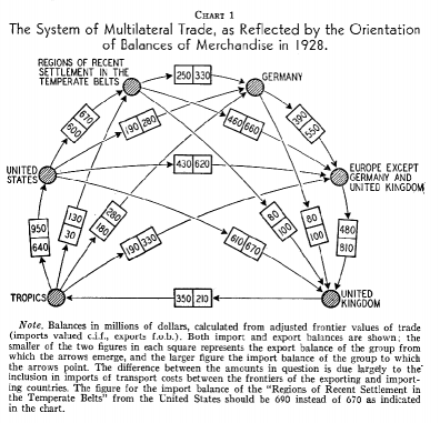
Figure 1: World Trade Network in 1928

Notes: This figured appeared in Folke Hilgerdt’s 1943 American Economic Review article “The case for multilateral trade”. The figure shows aggregate trade balances between selected large countries and different regions of the world. The paper includes a narrative discussion of how the patterns of trade depicted in weighted digraph drawn in the figure developed historically.

Source: Reproduced from Hilgerdt, (1943, Chart 1).

Although important exceptions exists, some highlighted below, economists historically avoided the study networks (see Figure 1). This is now changing, very quickly, and for several reasons. First, starting in the 1990s economic theorists applied the tools of game theory to formally study network formation (e.g., Jackson & Wolinsky,, 1996). In the resulting models agents add, maintain, and subtract links in order to maximize utility, with the realized network satisfying a pairwise stability equilibrium condition. Second, in parallel to this theoretical work, a lively empirical and methodological literature on peer group and neighborhood effects also arose (e.g., Manski,, 1993; Brock & Durlauf,, 2001; Graham,, 2008; Angrist,, 2014). Finally, largely driven by questions in empirical industrial organization, econometricians made substantial progress on the econometric analysis of games (cf., Bajari et al.,, 2013; de Paula,, 2013). Each of these literatures serve as foundations for material introduced below.

Outside of economics, two key initiators have been (i) the increasing availability of datasets with natural graph theoretic structure (see below for examples) and (ii) innovations in applied probability and theoretical statistics pertaining to random graph models (e.g., Diaconis & Janson,, 2008). These innovations provide a foundation upon which recent work in statistics and machine learning on networks is largely based.

A consequence of these developments is the emergence of a small methodological literature on the econometrics of networks. Empirical applications with substantial network content, spurred largely by access to new datasets, arose more quickly (e.g., Fafchamps & Minten,, 2002; De Weerdt,, 2004; Conley & Udry,, 2010; Atalay et al.,, 2011; Acemoglu et al.,, 2012; Banerjee et al.,, 2013; Barrot & Sauvagnat,, 2016). Furthermore, these applications now span the major fields of our discipline. Nevertheless many open questions in the econometrics of networks remain. In this chapter I attempt to provide an account of recent progress as well as make suggestions for future research. My audience is both econometricians and empirical researchers.

I divide my discussion into five parts. The discussion draws from recent contributions to the analysis of networks made in probability, econometrics, and statistics (including machine learning); approximately in that order. After an initial outline of recent empirical research with a network dimension in economics, Section 3 introduces some basic probability tools that will prove useful for what follows. Several of these tools are of quite recent origin. Next, in Sections 4 to 6 I turn to the analysis of dyadic regression models. Such models go back, at least, to the pioneering work of Tinbergen, (1962, Appendix VI) on gravity trade models. Although dyadic regression is a core empirical method in international trade, as well as in certain areas of political science and development economics, a coherent inferential foundation for empirical practice is only now emerging. My discussion, in addition to covering methods of inference, discusses how to incorporate unobserved heterogeneity into dyadic regression models (Section 6). Here I appropriate and extend insights from panel data (Chamberlain,, 1980, 1984, 1985; Hahn & Newey,, 2004; Arellano & Hahn,, 2007). This section also sketches out how to answer causal questions in dyadic settings.

Section 7 turns to the large network properties of several common network statistics. I focus on so-called network moments, or the frequencies with which certain low order subgraph configurations (e.g., triangles ) occur within a network. Subgraph counts, in the form of the triad census, were introduced by Holland & Leinhardt, (1970) almost a half-century ago. Recent developments in probability and statistics have substantially improved our understanding of these counts (e.g., Diaconis & Janson,, 2008; Bickel et al.,, 2011).

Subgraph counts may be of direct interest, but also serve as the building blocks of several popular network statistics, such as transitivity or moments of the degree distribution. Jackson et al., (2017) survey the mapping between different network statistics and economic phenomena and questions. My interest in network moments also stems from their value as inputs into structural model estimation in a manner akin to the way sample moments are paired with model moments in the simulated method of moments (e.g., Gourieroux et al.,, 1993). This idea is developed in Section 8.

The discussion of dyadic regression in Sections 4 to 6 rules out interdependencies in link formation. In dyadic models the utility two agents generate by forming a link is invariant to the presence or absence of links elsewhere in the network. Beginning with the seminal work of Jackson & Wolinsky, (1996), the relaxation of this assumption is a central preoccupation of both theoretical and econometric researchers. When link formation decisions are interdependent, inefficient network structures may occur in equilibrium, making policy analysis interesting. Empirical network formation models allowing for interdependencies are also challenging to study. In a typical model many equilibrium network configurations can arise for any given parameter value; such models are incomplete (e.g., Tamer,, 2003). In principle, standard tools developed in the context of economic games between a small number of agents apply. Practically speaking such methods are computationally infeasible in the many agent context of networks. Recent research proposes a variety of ways of getting around this conundrum.

Economists’ interest in networks stems from the belief that their structure is consequential. For example, Loury, (2002) argues that differences in social networks across Blacks and Whites drives, in part, racial inequality (cf., Graham, 2018b, ). Acemoglu et al., (2012) argue that the Leontief input-output structure of the economy shapes technology shock propagation. Alatas et al., (2016) show that network structure influences the flow and aggregation of information within rural villages. Theorists also study the interplay between network structure and agent behavior on that structure (Jackson & Yariv,, 2011; Jackson & Zenou,, 2015). Methodological research relating network structure to economic outcomes builds-upon the line of peer effects research initiated by Manski, (1993). The paper by Bramoullé et al., (2009) is a nice, and influential, example of recent work along such lines.

This survey, however, does not review methods for the empirical analysis of behavior on networks. Instead I focus on modeling their formation. My motivation for this emphasis is two-fold. First, Blume et al., (2011) already survey work at the intersection of peer group effect identification and networks (cf., Blume et al.,, 2015; de Paula,, 2017). Second, the current state of research in this area suggests that a better understanding of how networks form is a prerequisite for more credible research on their consequences.

Current research on the effects of network structure on outcomes largely treats it as exogenously given (although this is not always made explicit). This decision is one reason why research on peer effects and networks remains controversial a quarter century after Manski’s foundational paper. The focus maintained here, on formation, therefore seems to be a natural one. Ultimately, of course, the goal is to study the formation of networks and their consequences jointly, but such an integrated treatment remains largely aspirational at this stage. Although, Goldsmith-Pinkham & Imbens, (2013) provide one recent “proof of possibilities” example of such an integrated approach. Qu & Lee, (2015), Auerbach, (2016), Badev, (2017), and Johnsson & Moon, (2017) represent other steps in this direction.

2 Examples, questions and notation

The analysis of datasets with natural graph theoretic structure has a long history in the other social sciences (e.g., Moreno,, 1934), and more recently emerged as an area of focus within the statistics and machine learning community (e.g., Goldenberg et al.,, 2009; Kolaczyk,, 2009). Although we were late adopters, interest in these types of datasets now also extends across virtually all fields of economics. Nevertheless, as already noted, appropriate methods for the analysis of network data are not widely available. Ad hoc and/or heuristically motivated approaches to estimation and inference abound in empirical work. Networks are characterized by complex dependencies across agents, as well as other difficult modeling, estimation and inferential challenges. These challenges are just starting be understood and solved. Before discussing methods for the analysis of network data, I briefly introduce some recent examples of empirical network research in economics. These examples also serve to introduce some basic notation.

2.1 Empirical analysis of trade flows

Figure 2 visually depicts international trade in bananas, a widely-eaten tropical fruit, in 2015. Each dot or node in the figure corresponds to a country. If, for example, Honduras, exports at least 50,000 tons of bananas to the United States, then there exists a directed edge from Honduras to the United States. The exporting country (left node) is called the tail of the edge, while the importing country (right node) is its head. The set of all such exporter-importer relationships forms $G\left(\mathcal{V},\mathcal{E}\right)$, a directed network or digraph defined on $N=\left|\mathcal{V}\right|$ vertices or agents (here countries). The set $\mathcal{V}=\left\{1,\ldots,N\right\}$ includes all agents (countries) in the network and $\mathcal{E}\subseteq\mathcal{V}\times\mathcal{V}$ the set of all directed links (exporter-importer relationships of 50,000 tons or greater) among them. Let $N$ be the order of the digraph and $\left|\mathcal{E}\right|$ its size. In what follows nodes may be equivalently referred to as vertices, agents, individuals, countries and so on depending on the context. Likewise edges may be called links, friendships, ties, arcs, relationships and so on.

There are $N=220$ countries in the banana network and hence up to $2\tbinom{220}{2}=48,180$ directed trading relationships among them. How might an econometrician model the presence or absence of a trading relationship from country $i$ to $j$? Over fifty years ago Tinbergen, (1962, Appendix VI) introduced gravity models, suitable for data of the type shown in Figure 2. In a gravity model trade between two countries, a dyad in network parlance, is modeled as a function of exporter and importer attributes (e.g., their gross domestic products), as well as dyad-specific covariates (e.g., physical distance between them). Generalizations of Tinbergen’s approach are workhorses of modern empirical trade research (e.g., Santos Silva & Tenreyro,, 2006; Helpman et al.,, 2008; Anderson,, 2011).

Their ubiquity notwithstanding, serious open questions remain about how to estimate, and conduct inference on, the parameters of gravity trade models. Questions of particular interest here include how to account for the dependence across dyads sharing a country in common, how to incorporate country-specific (correlated) unobserved heterogeneity, and how to formalize causal policy effects in dyadic settings. As an example of the latter challenge, consider the effects of participation in multi-lateral trading agreements, such as the General Agreement on Tariffs and Trade (GATT) or its successor, the World Trade Organization (WTO), on trade flows. Does trade increase across participating countries (Rose,, 2004; Helpman et al.,, 2008)? While a mature literature on program evaluation suitable for single agent settings now exists (cf., Heckman & Vytlacil,, 2007; Imbens & Wooldridge,, 2009), a networked counterpart has yet to emerge.

2.2 Corporate governance

Next consider the affiliation network of (corporate board) directors and firms. This bipartite network $B\left(\mathcal{\mathcal{U}},\mathcal{V},\mathcal{E}\right)$ consists of two sets of agents, the set of possible directors, $\mathcal{U}$, and the set of firms, $\mathcal{V}$. Edges, $\mathcal{E}$, match directors to firms (i.e., corporate boards), and hence may only run between $\mathcal{V}$ and $\mathcal{U}$. A longstanding interest among corporate governance researchers centers on the implications of so-called board interlocks. When a single director sits on multiple corporate boards, then these corporations have interlocking directorates (Dooley,, 1969). Interlocking directorships may facilitate collusion and other anti-competitive activities as well as, perhaps more positively, the diffusion of innovations in corporate governance (Davis,, 1991, 1996).

Figure 3 plots the one-mode projection of the directors-to-firms bipartite network for S&P 1,500 firms in 2016. This projection generates an undirected network $G\left(\mathcal{V},\mathcal{E}\right)$ on the set of all firms, with an edge between any two firms sharing at least one director in common (i.e., with interlocking corporate boards). Large firms in United States are inter-connected via overlapping corporate board membership. On average firms share at least one board member in common with four other firms and over 80 percent of S&P 1,500 firms form a giant connected component of board interlocks. The board interlock network is also highly transitive: two firms are much more likely to share a director in common, if they also share one in common with a third firm.

Chu & Davis, (2016) and Gualdani, ming provide recent analyses of board interlocks as well as references to earlier work.

2.3 Production networks

Atalay et al., (2011) study the production network of the United States economy. The sale and purchase of intermediate inputs between firms joins virtually all publicly traded corporations in the United States into one giant buyer-supplier network.

Serpa & Krishnan, (2017) present evidence of productivity spillovers across firms linked together via supply chain relationships (cf., Acemoglu et al., 2016a, ). Acemoglu et al., (2012) study the effect of the Leontief input-output structure of the US economy on shock propagation. Their analysis suggests that idiosyncratic technology shocks to critical input suppliers may have macro-level effects.

Bernard et al., (2018), using detailed supply-chain data from Japan, show how lowering supplier search costs allows firms to source inputs more efficiently, in turn lowering marginal production costs. The rich supply-chain data underlying the analysis of Bernard et al., (2018) is emblematic of the increasing availability of detailed supply chain network data from different countries (e.g., Dhyne et al.,, 2015). These datasets have the potential to dramatically improve our understanding of, for example the sources of heterogeneity in productivity across firms (e.g., Atalay et al.,, 2014) and the upstream and downstream implications of (horizontal) mergers (e.g., Fee & Thomas,, 2004; Bhattacharya & Nain,, 2011; Ahern & Harford,, 2014), among many other areas of industrial organization and regulation policy.

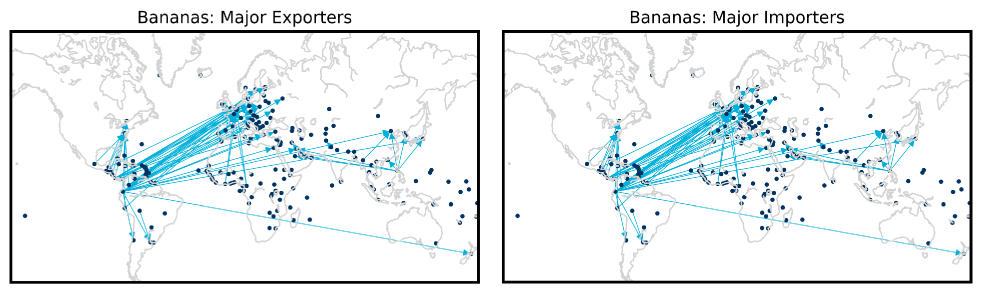
Figure 2: World Trade in Bananas, 2015

Source: BACI-CEPII International Trade Database (cf., Gaulier & Zignago,, 2010; De Benedictis et al.,, 2014) and author’s calculations.

Notes: International trade of bananas in 2015 (HS6 code 080390). Each node in the figure represents a country (nodes are positioned at capital cities) and an edge between two nodes indicates the presence of at least 50,000 tons of directed banana flows (the head of each directed edge corresponds to the importing nation). In the left-hand panel node size is proportional to the total exports of bananas by the relevant nation, while in the right it is proportional to its total imports.

2.4 Research collaboration

Jaffe, (1986), in a classic study, presented evidence of research and development (R&D) spillovers across technologically adjacent firms (Bloom et al.,, 2013; Acemoglu et al., 2016b, ). Such spillovers provide a motivation for firms to undertake collaborative R&D, a tendency which has increased over time (Hagedoorn,, 2002; Tomasello et al.,, 2017). König et al., (2019) model the formation of R&D partnerships across firms theoretically and empirically, exploring the implications of network structure for optimal R&D subsidy policies. The structure of spillovers across firms, as well as the mechanisms whereby they form R&D partnerships, determines optimal policies.

Ductor et al., (2014) study collaboration and research output among and across economists. Newman, (2001) explores collaboration networks in the various sciences.

2.5 Risk-sharing across households

A classic question in development economics is whether households efficiently share risk through informal agreements (Townsend,, 1994; Udry,, 1994). Recently economists have directly collected information on risk-sharing relationships across households. For example, De Weerdt, (2004) collected data on risk-sharing links across households in a village in Tanzania and empirically modeled the determinants of these links (cf., Fafchamps & Lund,, 2003; Fafchamps & Gubert,, 2007). Ambrus et al., (2014) investigate how the precise structure of links across households determines the amount of risk that can be insured, as well as the form of second best, more local, network structures.

Network structure now informs many other areas of development economics, including research on technology adoption and program take-up in rural settings (e.g., Banerjee et al.,, 2013; Kim et al.,, 2015), the productivity of small traders and firms (e.g., Fafchamps & Minten,, 2002), and post-migration employment outcomes (Beaman,, 2011; Munski,, 2003), among other examples.

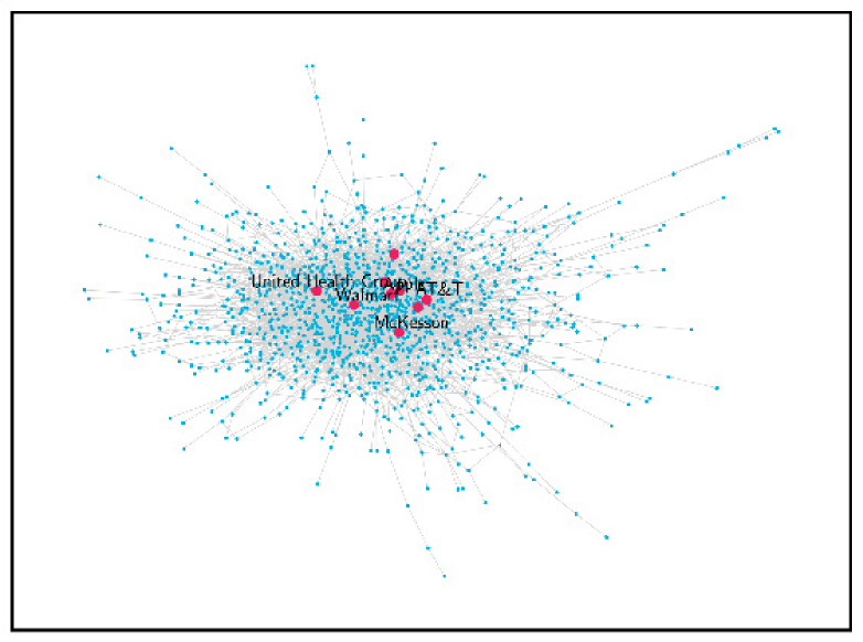
Figure 3: United States Corporate Board Interlocks, 2016

Source: Wharton Research Data Services (WRDS) - Institutional Shareholder Services (ISS) Directors dataset and author’s calculations (cf., Chu & Davis,, 2016).

Notes: The figure plots the largest connected component of the corporate board interlock network in 2016 among S&P 1,500 firms. The top 10 Fortune 500 firms in 2016 are the larger ‘Rose Garden’ colored nodes. A total of 1,216 firms belong to the largest connected component. See Newman, (2010, p. 124 - 127) for details on how to construct one-mode projections of bipartite graphs.

2.6 Insurer-provider and referral networks for healthcare

Many features of the health care market naturally map into graphs. For example, physicians may have admitting privileges across multiple hospitals, insurers typically offer preferential terms to selected networks of providers, and doctors vary in the intensity with which they refer patients to one another.

The welfare and economic implications of these networks are likely immense, given the magnitude of the health care sector in the United States economy. Ho, (2009) represents one attempt to grapple with the network structure of healthcare markets.

2.7 Employment search

Ioannides & Loury, (2004) survey the substantial literature on the interplay between social networks and job acquisition, a topic that has fascinated both sociologists and economists at least since Granovetter, (1973). The growing availability of longitudinal register data from various countries provides an opportunity to study the interface between networks and inequality in the labor market more carefully.

For example, Saygin et al., (2014) use the Austrian Social Security Database to construct a co-worker network for middle aged workers in Austria. A co-worker is anyone who an individual has ever worked with previously. They find that the structure of these co-worker networks predict the ease with which workers find employment after establishment closures (i.e., mass layoffs). This paper provides a nice example of how new data may facilitate the re-visiting of a classic networks question (cf., Hensvik & Skans,, 2016).

2.8 Questions

The examples outlined above represent only a small sample of recent appearances of network data in empirical economic research. What do we hope to learn from this growing body of research? As noted in the introduction, empirical research on networks can usefully be divided between that which studies the consequences of networks and that which studies their formation. The premise of this chapter is that network linkages across agents are consequential. That is, I take as given that networks are important venues for shock propagation, information diffusion, learning and various types of peer interactions. Maintaining this premise justifies my focus on the econometric modeling of network formation.

An analogy with the development of single agent models of discrete choice is useful. McFadden, (1974), in a pioneering paper, initiated a research program on identifying and estimating random utility models of discrete choice. Empirical application, computation, semiparametric identification and estimation, the inclusion of unobserved choice attributes, and allowing for strategic behavior, all have been important accomplishments of this research program. These econometric models are, in turn, routinely used in virtually all areas of economics.

The goal here is analogous. Relational data are ubiquitous in economics, but econometric models for such data are not. The goal, therefore, is to develop models for these data, preferably with (i) strong microeconomic foundations, (ii) that allow for unobserved agent-level heterogeneity, and (iii) incorporate interdependencies in preferences over links. Also required are feasible methods of estimation and inference (and in this area interesting and challenging questions are abundant). The availability of econometric methods for network analysis will, in turn, allow for counterfactual policy and welfare analysis. How would a particular horizontal merger affect upstream supply chain structure? What is the effect on trade flows of Eurozone membership? Could a school principal increase friendships across races, or raise average achievement, by structuring classrooms under her purview differently?

Some readers may wish to skip Section 3 initially and instead start with Sections 4 to 6. They could then return to Section 3 before tackling Sections 7 and 8. Graph theoretic concepts and notation appears throughout the chapter. While many terms and definitions are formally defined, others are not. Missing definitions can be found in any basic graph theory textbook.

3 Basic probability tools: random graphs, graphons, graph limits and sampling

This section provides an informal introduction to key ideas from the applied probability literature on exchangeable random graphs. The main concepts are (i) exchangeable random graphs and their representation, (ii) subgraph densities or network moments, (iii) limits of sequences of exchangeable random graphs, and (iv) sampling. These ideas underlie a substantial share of recent research on the statistics of networks (e.g., Airoldi et al.,, 2008; Diaconis et al.,, 2008; Bickel & Chen,, 2009; Bickel et al.,, 2011; Bhamidi et al.,, 2011; Chatterjee et al.,, 2011; Olhede & Wolfe,, 2014; Orbanz & Roy,, 2015; Gao et al.,, 2015).

Much of this statistics work has been motivated by research questions in computational biology and neuroscience (e.g., Picard et al.,, 2008). Link formation in these settings is not driven by purposeful agents. Consequently this research may initially appear rather distant from the concerns of econometricians. Nevertheless my view is that recent developments in probability and statistics have much to offer econometricians interested in networks (and also vice-versa, although making this second argument this is not on my agenda here).

The basic concepts introduced in this section appear frequently in later portions of the chapter.

3.1 Notation

Let $G\left(\mathcal{V},\mathcal{E}\right)$ be a finite undirected network or graph defined on $N=\left|\mathcal{V}\left(G\right)\right|$ vertices or agents; here $\mathcal{V}\left(G\right)=\left\{1,\ldots,N\right\}$ denotes the set of all agents in the network. Any two agents may be connected or not. The set of such links is recorded in the edge list $\mathcal{E}\left(G\right)=\left\{\left(i,j\right),\left(k,l\right),\ldots\right\}$, consisting of the (unordered) indices of all connected agent pairs. Call $N$ the order of the network and $\left|\mathcal{E}\left(G\right)\right|$ its size. We can represent $G\left(\mathcal{V},\mathcal{E}\right)$ by the $N\times N$ adjacency matrix $\mathbf{D}=\left[D_{ij}\right]_{i,j\in\mathcal{V}\left(G\right)}$ with $ij^{th}$ element

$$D_{ij}=\left\{\begin{array}[]{cl}1,&\left(i,j\right)\in\mathcal{E}\left(G\right)\\ 0,&\text{otherwise}\end{array}\right..$$

For an undirected network, with self-ties or loops ruled out, such that $D_{ii}=0$ for $i\in\mathcal{V}\left(G\right)$, $\mathbf{D}$ is a symmetric binary matrix with a diagonal of structural zeros. I focus on undirected networks initially, but also present some results for directed networks and bipartite networks. Specific notation for these special cases will be introduced as needed.

In settings where it is useful to emphasize the order of $G$, I use the notation $G_{N}$. This is especially useful when considering sequences of graphs. Let $\left(i,j\right)\in\mathcal{E}\left(G\right)$ be an edge in $G$; sometimes I will abbreviate $\left(i,j\right)$ as $ij$. The complete graph on $p$ vertices is denoted by $K_{p}$.

Following Jackson, (2008), let $G-ij$ denote the network obtained by deleting edge $ij$ from $G$ (if present), and $G+ij$ the network one gets after adding this link. Let $\mathbf{D}\pm ij$ denote the adjacency matrix associated with the network obtained by adding/deleting edge $\left(i,j\right)$ from $G$. Let $\mathbb{D}_{N}$ denote the set of all $2^{\binom{N}{2}}$ possible adjacency matrices and $\mathbb{I}_{N}$ the set of all possible $N$-dimensional binary vectors.

Let $N\left(i\right)=\left\{j\in\mathcal{V}\thinspace:\thinspace ij\in\mathcal{E}\right\}$ be the set of agent $i$’s neighbors: agents to which she is directly linked. The degree of agent $i$ is given by the cardinality of this set. Equivalently agent $i$’s degree may be computed by summing the elements of the $i^{th}$ row of the adjacency matrix. Let $\iota_{N}$ be an $N\times 1$ vector of ones. The vector $\mathbf{D}_{+}=\mathbf{D}\iota_{N}$ is called the degree sequence of the network (typically we re-arrange the order of agents such that the elements of this vector are in ascending order).

I informally call a network dense if its size, or number of edges, is “close to” $N^{2}$ and sparse if its size is “close to” $N$. More precisely a sequence of graphs is sparse in the limit if the number of edges in it grows linearly with $N$, dense if this growth is quadratic.

There are $n\overset{def}{\equiv}\tbinom{N}{2}=\frac{1}{2}N\left(N-1\right)$ pairs of agents, or dyads, in a network consisting of $N$ agents. Triples, quadruples and quintuples of agents are call triads, tetrads and pentads respectively. A tuple of 17 agents, which arises rather rarely in everyday empirical work, is evidently called a septendecuple. Not having formally studied Latin, I offer the reader no guidance on pronunciation.

Let $\sum_{i<j}$ be shorthand for $\sum_{i=1}^{N-1}\sum_{j=i+1}^{N}$ with $\sum_{i<j<k}$ similarly defined. The density of a network,

$$P_{N}\left(\vbox{\hbox{\includegraphics[scale={0.1250}]{edge}}}\right)\overset{def}{\equiv}\hat{\rho}_{N}\overset{def}{\equiv}\frac{2}{N\left(N-1\right)}\sum_{i<j}D_{ij},$$

equals the proportion of connected dyads. Let $D_{i+}$ be the $i^{th}$ element of the degree sequence. Average degree,

$$\hat{\lambda}_{N}\overset{def}{\equiv}\left(N-1\right)\hat{\rho}_{N}\overset{def}{\equiv}\frac{1}{N}\sum_{i=1}^{N}D_{i+},$$

equals the average number of links per agent in the network.

In what follows random variables are (generally) denoted by capital Roman letters, specific realizations by lower case Roman letters and their support by blackboard bold Roman letters. That is $Y$, $y$ and $\mathbb{Y}$ respectively denote a generic random draw of, a specific value of, and the support of, $Y$. The abbreviations i.i.d., CLT , LLN and GGP stand for, respectively, “independent and identically distributed”, “central limit theorem”, “law of large numbers” and “graph generating process”. For the vector $\mathbf{b}$, $\left\|\mathbf{b}\right\|_{2}$ denotes the Euclidean norm; for the matrix $\mathbf{B}$, $\left\|\mathbf{B}\right\|_{F}$ denotes the Frobenius norm. I use $I_{N}$ to denote the $N\times N$ identity matrix. $\mathbb{N}$ denotes the set of natural numbers and $\left[Y_{ij}\right]_{i,j\in\mathbb{N}}$ an infinite two-dimensional array with $ij^{th}$ element $Y_{ij}$.

I use the big-Omega notation $X_{N}=\Omega\left(Y_{N}\right)$ to denote that $X_{N}=O\left(Y_{N}\right)$ and $Y_{N}=O\left(X_{N}\right)$. The notation $\overset{D}{=}$ denotes equality in distribution, $\overset{def}{\equiv}$ a mathematical definition. Let $\theta$ be some parameter value in the space $\Theta$. Let $S_{N}\left(\theta\right)$ be some statistic indexed by this parameter with population value $\theta_{0}$. I let $S_{N}=S_{N}\left(\theta_{0}\right)$ denote the statistic evaluated at $\theta=\theta_{0}$. To economize on space I sometimes abbreviate $\Pr\left(\left.Y=y\right|X=x\right)$ as $\Pr\left(\left.Y=y\right|x\right)$ or $\Pr\left(\left.y\right|x\right)$ and similarly for $\mathbb{E}\left[\left.Y\right|x\right]$, $\mathbb{V}\left(\left.Y\right|x\right)$ etc.

3.2 Exchangeable random graphs

Initially assume the unavailability of agent-specific covariates, making it natural to assume that agents are exchangeable (models with covariates, and a correspondingly weaker notion of exchangeability, feature in Sections 4, 5, 6 and 8). Let $\pi:\left\{1,\ldots,N\right\}\mapsto\left\{1,\ldots,N\right\}$ be a permutation of the node labels of $G\left(\mathcal{V},\mathcal{E}\right)$ and $\Pi$ the set of all such permutations. The random graph $G$ is jointly exchangeable if

$$\left[D_{ij}\right]\overset{D}{=}\left[D_{\pi\left(i\right)\pi\left(j\right)}\right]$$ (1)

for every permutation $\pi\in\Pi$.

In settings where node labels have no meaning, exchangeability is an implication of a priori researcher belief (and hence a natural modeling assumption). Consider a researcher analyzing the adjacency matrix associated with a set of friendship links among adolescents in a high school (e.g., Currarini et al.,, 2009), in the absence of node-specific covariates, there is no reason to change one’s modeling approach after simultaneously applying a particular reshuffling of agents to both the rows and columns of $\mathbf{D}$ (cf., Rubin,, 1981). Put differently, when node labels have no meaning, the probability attached to any isomorphism of $G$ should be the same as that attached to $G$ itself.

There are many interesting statistics of $\mathbf{D}$ which are invariant to simultaneous row and column permutations. Examples include a network’s density, diameter and triangle $(\vbox{\hbox{\includegraphics[scale={0.125}]{triangle}}})$ count. A family of such statistics, network moments, is introduced below. Exchangeability suggests that a statistical model should attach different probabilities to networks with different values of such (permutation invariant) statistics, but the same probability to two networks which are isomorphic (which will share common values of any permutation invariant statistic).

An exchangeable model with strategic interaction

Most extant models of network formation satisfy condition (1). As an example, which will help to fix some ideas, consider the model of strategic network formation with bilateral transfers studied by Graham & Pelican, (2020). Let $\nu_{i}\thinspace:\thinspace\mathbb{D}_{N}\rightarrow\mathbb{R}$ be a utility function for agent $i$, which maps networks into utility. Define the marginal utility of edge $ij$ for agent $i$ as

$$MU_{ij}\left(\mathbf{D}\right)=\left\{\begin{array}[]{cc}\nu_{i}\left(\mathbf{D}\right)-\nu_{i}\left(\mathbf{D}-ij\right)&\text{if}\thinspace D_{ij}=1\\ \nu_{i}\left(\mathbf{D}+ij\right)-\nu_{i}\left(\mathbf{D}\right)&\text{if}\thinspace D_{ij}=0\end{array}\right..$$ (2)

From Bloch & Jackson, (2006), a network is pairwise stable with transfers if the following condition holds.

Definition 1.

(Pairwise stability with Transfers) The network $G\left(\mathcal{V},\mathcal{E}\right)$ is pairwise stable with transfers if
(i) $\forall\left(i,j\right)\in\mathcal{E}\left(G\right),\thinspace MU_{ij}\left(\mathbf{D}\right)+MU_{ji}\left(\mathbf{D}\right)\geq 0$
(ii) $\forall\left(i,j\right)\notin\mathcal{E}\left(G\right),\thinspace MU_{ij}\left(\mathbf{D}\right)+MU_{ji}\left(\mathbf{D}\right)<0$

If the network in hand is a pairwise stable one, then any links actually present generate (weakly) positive utility (on net for the two agents on each side of a link). Unobserved links, in contrast, would not generate net positive utility if present.

Graham & Pelican, (2020) focus on a general family of parametric utility functions which includes, among others, the specification

$$\nu_{i}\left(\mathbf{\left.d\right|}\mathbf{A},\mathbf{B},\mathbf{V^{*}};\gamma_{0}\right)=\sum_{j}d_{ij}\left[A_{i}+B_{j}+\gamma_{0}\left(\sum_{k}d_{ik}d_{jk}\right)-V_{ij}^{*}\right]$$ (3)

with $\mathbf{V^{*}}=\left[V_{ij}^{*}\right]$ , $\mathbf{A}=\left[A_{i}\right]$ and $\mathbf{B}=\left[B_{i}\right]$. Under (3), assuming $\gamma_{0}>0$, dyad $\left\{i,j\right\}$ will generate more utility when forming a link if they already share many links or “friends” in common (i.e., if $\sum_{k}d_{ik}d_{jk}$ is large). Here $A_{i}$ and $B_{j}$ are agent-specific “extroversion” and “popularity” parameters, the effect of which is to generate degree heterogeneity (cf., Graham,, 2017). The term $V_{ij}^{*}$ is an idiosyncratic dyad-specific utility shifter. Graham & Pelican, (2020) leave the joint distribution of $\mathbf{A}$ and $\mathbf{B}$ unrestricted, but here I will assume that $\left\{\left(A_{i},B_{i}\right)\right\}_{i=1}^{N}$ is an i.i.d. sequence which is independent of $\left\{\left(V_{ij}^{*},V_{ji}^{*}\right)\right\}_{i,j\in\left\{1,\ldots,N\right\},i<j}$, also assumed i.i.d.

When the utility function is of the form given in (3) the marginal utility agent $i$ gets from a link with $j$ is

$$MU_{ij}\left(\left.\mathbf{d}\right|\mathbf{A},\mathbf{B},\mathbf{V^{*}};\gamma_{0}\right)=A_{i}+B_{j}+\gamma_{0}\left(\sum_{k}d_{ik}d_{jk}\right)-V_{ij}^{*}.$$

Pairwise stability then implies, conditional on the realizations of $\mathbf{A}$, $\mathbf{B}$, $\mathbf{V^{*}},$ and the value of externality parameter, $\gamma_{0}$, that the observed network must satisfy, for $i=1,\ldots,N-1$ and $j=i+1,\ldots,N$

$$D_{ij}=\mathbf{1}\left(U_{i}+U_{j}+2\gamma_{0}\left(\sum_{k}D_{ik}D_{jk}\right)\geq V_{ij}\right)$$ (4)

with $U_{i}=A_{i}+B_{i}$ and $V_{ij}=V_{ij}^{*}+V_{ji}^{*}$. Equation (4) defines a system of $\tbinom{N}{2}=\frac{1}{2}N\left(N-1\right)$ nonlinear simultaneous equations. Any solution to this system – and there will typically be multiple ones – constitutes a pairwise stable (with transfers) network.

As written, model (4) is incomplete (cf., de Paula,, 2013). Even if we assume that the observed network is a pairwise stable one, we have not specified a mechanism for selecting, when there are multiple ones, a specific equilibrium configuration. To complete the model, following the more careful development in Pelican & Graham, (2019), let $\mathcal{N}_{\mathbf{d}}\left(\mathbf{V};\mathbf{U},\gamma\right)$ equal the probability that configuration $\mathbf{D}=\mathbf{d}$ is selected. If $\mathbf{d}$ is not an equilibrium – given $\mathbf{U}$, $\mathbf{V}$ and $\gamma$ – then $\mathcal{N}_{\mathbf{d}}\left(\mathbf{V};\mathbf{U},\gamma\right)=0$. If $\mathbf{d}$ is the unique equilibrium then $\mathcal{N}_{\mathbf{d}}\left(\mathbf{V};\mathbf{U},\gamma\right)=1$. If $\mathbf{d}$ is one of several equilibria, then $0\leq\mathcal{N}_{\mathbf{d}}\left(\mathbf{V};\mathbf{U},\gamma\right)\leq 1$ etc.

For $\mathbb{D}_{N}$ the net of all $N\times N$ undirected adjacency matrices, we have that $\sum_{\mathbf{d}\in\mathbb{D}_{N}}\mathcal{N}_{\mathbf{d}}\left(\mathbf{V};\mathbf{U},\gamma\right)=1$. The conditional likelihood of observing network wiring $\mathbf{D}=\mathbf{d}$ is therefore

$$\Pr\left(\left.\mathbf{D}=\mathbf{d}\right|\mathbf{U};\gamma\right)=\int_{\mathbf{v}\in\mathbb{R}^{n}}\mathcal{N}_{\mathbf{d}}\left(\mathbf{v};\mathbf{U},\gamma\right)f_{\mathbf{V}}\left(\mathbf{v}\right)\mathrm{d}\mathbf{v}.$$

The $\tbinom{N}{2}$ equilibrium conditions (4) indicate that if $\mathbf{d}=\left[d_{ij}\right]$ is an equilibrium, then so is $\mathbf{d}_{\pi}\overset{def}{\equiv}\left[d_{\pi\left(i\right)\pi\left(j\right)}\right]$. Hence as long as the equilibrium selection mechanism is also invariant to index permutations, as is natural to require, condition (1) holds.

Under the null of no strategic interaction, $\gamma=0$, the likelihood simplifies to

$$\Pr\left(\left.\mathbf{D}=\mathbf{d}\right|\mathbf{U};0\right)=\int_{\mathbf{v}\in\mathbb{R}^{n}}\mathcal{N}_{\mathbf{d}}\left(\mathbf{v};\mathbf{U},0\right)f_{\mathbf{V}}\left(\mathbf{v}\right)\mathrm{d}\mathbf{v}$$ (5)

with

$$\mathcal{N}_{\mathbf{d}}\left(\mathbf{v};\mathbf{U},0\right)= \prod_{i=1}^{N-1}\prod_{j=i+1}^{N}\mathbf{1}\left(U_{i}+U_{j}\geq v_{ij}\right)^{d_{ij}}$$

$$\times\mathbf{1}\left(U_{i}+U_{j}<v_{ij}\right)^{1-d_{ij}}.$$

Since $\left\{\left(V_{ij}\right)\right\}_{i,j\in\left\{1,\ldots,N\right\},i<j}$ is i.i.d., if we further assume that $f_{V_{12}}\left(v\right)=e^{v}/\left[1+e^{v}\right]^{2}$, the logistic density, explicitly evaluating the integral in (5) yields

$$\Pr\left(\left.\mathbf{D}=\mathbf{d}\right|\mathbf{U};0\right)=\prod_{i=1}^{N-1}\prod_{j=i+1}^{N}\left[\frac{\exp\left(U_{i}+U_{j}\right)}{1+\exp\left(U_{i}+U_{j}\right)}\right]^{d_{ij}}\left[\frac{1}{1+\exp\left(U_{i}+U_{j}\right)}\right]^{1-d_{ij}},$$ (6)

which is the likelihood associated with the so-called $\beta$-model of Frank, (1997) and Chatterjee et al., (2011).

A feature of the $\beta$-model is that links form independently conditional on the latent agent-specific effects $\left\{U_{i}\right\}_{i=1}^{N}$. Equation (6) consists of a product of $\tbinom{N}{2}$ conditionally independent likelihood contributions.

Evidently, this conditional independence structure is not typically a feature of the model when $\gamma>0$, such that strategic interaction is present. To see why by means of a simple example, consider a network consisting of just three homogenous agents (i.e., $U_{1}=U_{2}=U_{3}=0$). Initially assume that both $V_{12}$ and $V_{13}$ are less then zero, but that $0<V_{23}\leq 2\gamma_{0}$. This corresponds to edges $\left(1,2\right)$ and $\left(1,3\right)$ generating so much intrinsic utility that they will form irrespective of what other edges may or may not be present in the network. In contrast, the intrinsic utility attached to edge $\left(2,3\right)$ falls in an intermediate range: the edge forms if edges $\left(1,2\right)$ and $\left(1,3\right)$ are present – such that agents $2$ and $3$ share agent $1$ as a friend in common – and does not form if they are absent. This configuration of utility shocks is depicted in the left-hand panel of Figure 4. The unique equilibrium outcome in this case is a triangle $\left(\vbox{\hbox{\includegraphics[scale={0.125}]{triangle}}}\right)$ network.

If, instead, $V_{12}$ and $V_{13}$ are both greater than $2\gamma$, such that the $\left(1,2\right)$ and $\left(1,3\right)$ edges never form because of their low intrinsic utility (again irrespective of what other edges may or may not be present in the network), then the $\left(2,3\right)$ edge will not form either. This scenario is depicted in the right-hand panel of Figure 4. The unique equilibrium outcome in this case is an empty $\left(\vbox{\hbox{\includegraphics[scale={0.125}]{empty}}}\right)$ network.

This simple example shows that $D_{23}$ need not vary independently of $D_{12}$ and $D_{13}$ conditional on $\left(U_{1},U_{2},U_{3}\right)$ in the presence of strategic interaction ($\gamma>0$) . Such conditional independence is a feature of the $\beta$-model ($\gamma=0$). While the model is exchangeable both when $\gamma>0$ and when $\gamma=0$, the conditional independence of edges only obtains under the no strategic interaction null.

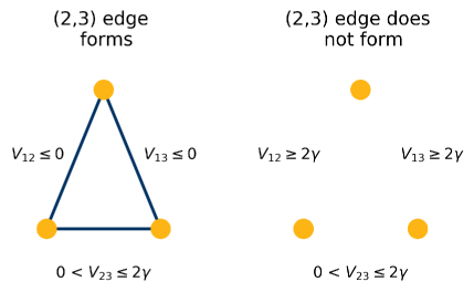
Figure 4: Dependent link formation

Notes: Both panels depict the unique pairwise stable equilibrium associated with the shown triple of dyad-level utility shifters $V_{12}$, $V_{13}$ and $V_{23}$ and agent-level heterogeneity parameters $U_{1}$, $U_{2}$ and $U_{3}$ identically equal to zero. In both panels the realized value of $V_{23}$ is the same, but whether $D_{23}=1$ or $0$ varies with the realized values of $V_{12}$ and $V_{13}$. If $V_{12}$ and $V_{13}$ are sufficiently low, then $D_{23}=1$; if they are sufficiently high, then $D_{23}=0$. Links are not conditionally independent given $\left\{U_{i}\right\}_{i=1,2,3}$.

3.3 Conditionally independent dyad (CID) models and the graphon

Having established that a network probability model should satisfy the joint exchangeability condition (1), it is important to articulate classes of models that do so. One such family of models, suggested by the last example, are conditionally independent dyad (CID) models (Chandrasekhar,, 2015; Shalizi,, 2016). In these models each agent is characterized by an unobserved latent attribute, $U_{i}$. The $N$ agents in the network in hand are viewed as independent random draws from some population, such that the $\left\{U_{i}\right\}_{i=1}^{N}$ are independently and identically distributed. Conditional on the agent-specific latent variables $\mathbf{U}=\left(U_{1},\ldots,U_{N}\right)^{\prime}$ edges form independently with

$$\left.D_{ij}\right|U_{i},U_{j}\sim\mathrm{Bernoulli}\left(h\left(U_{i},U_{j}\right)\right),$$

for every dyad $\left\{i,j\right\}$ with $i<j$. Here $h\left(u,v\right)=h\left(v,u\right)$ for all $\left(u,v\right)\in\mathbb{U}\times\mathbb{U}$ is a symmetric edge probability function. In anticipation of results to come, call this function a graphon: short for graph function.

Conditional on the latent agent-specific effects the likelihood of the network is

$$\Pr\left(\left.\mathbf{D}=\mathbf{d}\right|\mathbf{U}=\mathbf{u}\right)=\prod_{i<j}h\left(u_{i},u_{j}\right)^{d_{ij}}\left[1-h\left(u_{i,}u_{j}\right)\right]^{1-d_{ij}}.$$

Unconditional on $\mathbf{U}$, the likelihood equals

$$\Pr\left(\mathbf{D}=\mathbf{d}\right)=\int\cdots\int\left\{\prod_{i<j}h\left(u_{i},u_{j}\right)^{d_{ij}}\left[1-h\left(u_{i,}u_{j}\right)\right]^{1-d_{ij}}\right\}\prod_{i=1}^{N}f_{U}\left(u_{i}\right)\mathrm{d}u_{i},$$ (7)

where $f_{U}\left(u\right)$ is the density of $U$. Importantly (7) allows for dependence across dyads which share agents in common. Independence holds only conditional on the latent agent attributes (Graham,, 2017). Similar independence restrictions play a prominent role in the econometrics of panel data (Chamberlain,, 1984; Arellano & Honoré,, 2001).

It is an easy exercise to show that (7) is compatible with the finite joint exchangeability restriction (1).

The $\beta$-model, introduced above, belongs to the family of CID models with a graphon of

$$h\left(u,v\right)=\frac{\exp\left(u+v\right)}{1+\exp\left(u+v\right)}.$$

Random threshold graphs (e.g., Diaconis et al.,, 2008) are also members of this family with graphon

$$h\left(u,v\right)=\mathbf{1}\left(F_{U}\left(u\right)+F_{U}\left(v\right)\geq\alpha\right),$$

and $F_{U}\left(u\right)$ the CDF of $U$.

It is important to realize that CID models constitute only a subset of all jointly exchangeable random graph models when $N$ – the number of agents in the network – is finite. As shown by means of the example introduced above, strategic interaction in link formation can induce dependence across elements of the adjacency matrix that evidently cannot be eliminated by conditioning (see Figure 4 above). Although not all exchangeable models are CID ones, this family of models plays an outsized role in extant large sample theory for networks.

3.4 Aldous-Hoover representation theorem and the graphon

Joint exchangeability imposes more structure on the network probability distribution when there are an infinite number of agents. Specifically, if we strengthen (1) to hold for any permutation of a finite number of the indices of the infinite sequence $\mathbb{N}=\left\{1,2,3,\ldots\right\}$, we have a generalization of de Finetti, (1931) type exchangeability of an infinite sequence, appropriate for infinite random graphs. In independent work Aldous, (1981) and Hoover, (1979) showed the following representation result for infinite random adjacency matrices (cf., Kallenberg,, 2005).

Theorem 1.

(Aldous-Hoover) A random adjacency matrix $\left[D_{ij}\right]_{i,j\in\mathbb{N}}$ is jointly exchangeable if and only if there is a measurable function $g:\left[0,1\right]^{4}\rightarrow\left\{0,1\right\}$ such that

$$\left[D_{ij}\right]\overset{D}{=}\left[g\left(\alpha,U_{i},U_{j},V_{ij}\right)\right]$$

for $\alpha$, $\left\{U_{i}\right\}_{i\in\mathbb{N}}$ , and $\left\{V_{ij}\right\}_{i,j\in\mathbb{N},i<j}$ independently and identically distributed $\mathcal{U}\left[0,1\right]$ random variables with $V_{ij}=V_{ji}$.

Here $\alpha$ is a mixing parameter, analogous to the one appearing in de Finetti’s (1931) classic representation theorem for exchangeable binary sequences. Theorem 1 implies that if network agents are exchangeable for all $N$, then we can proceed ‘as if’ edges formed according to a CID model or a mixture of such models.

Exploiting the fact that the elements of $\mathbf{D}$ are binary, we can simplify Theorem 1 as follows. Averaging over $V_{ij}$ yields

$$h\left(\alpha,u_{i},u_{j}\right) \overset{def}{\equiv}\int_{0}^{1}g\left(\alpha,u_{i},u_{j},v\right)\mathrm{d}v$$

from which we get the more convenient representation, for $i<j$,

$$\left[D_{ij}\right]\overset{D}{=}\left[\mathbf{1}\left(V_{ij}\leq h\left(\alpha,U_{i},U_{j}\right)\right)\right].$$ (8)

This is, of course, just a conditional edge independence model (or, more precisely, a mixture of such models). In what follows I focus on inference which conditions on the empirical distribution of the data; consequently $\alpha$ can often safely be ignored. When this is the case I suppress the $\alpha$ argument in the graphon, writing $h\left(U_{i},U_{j}\right)$. See Bickel & Chen, (2009) and Menzel, (2017) for additional discussion.

Theorem 1 motivates an approach to nonparametric modeling of large networks that proceeds ‘as if’ links form independently conditional on the agent-specific latent variables $\mathbf{U}=\left(U_{1},\ldots,U_{N}\right)^{\prime}$. This is convenient because CID models induce a very particular dependence structure across the rows and columns of the network adjacency matrix.

Consider, without loss of generality, agents $1$, $2$ and $3$. In a CID model $D_{12}$ and $D_{13}$ may covary; the dyads $\left\{1,2\right\}$ and $\left\{1,3\right\}$ share the agent $1$ in common and hence both links form, in part, based on the value of $U_{1}$. However $D_{12}$ and $D_{13}$ vary independently conditional on $U_{1}$, $U_{2}$ and $U_{3}$ (hence the conditionally independent dyad nomenclature). Links involving pairs of dyads which share no agents in common, for example $D_{12}$ and $D_{34}$, form independently.

The structured pattern of dependence, independence and conditional independence associated with CID models facilitates the development of LLNs and CLTs that can be applied to statistics of the adjacency matrix. A group of statistics for which some large network distribution theory is available are network moments.

3.5 Network moments

Almost fifty years ago Holland & Leinhardt, (1970) suggested that a network’s architecture could be usefully summarized by its average local structure. Agent exchangeability, in conjunction with Theorem 1, also motivates an approach to network modeling based on the frequency of low order subgraph configurations (i.e., the number of edges, two stars, triangles, squares, k-stars etc).

Consider, for example, the set of all $\tbinom{N}{3}$ triads – unordered triples of agents – in a network; what fraction of these triads take two-star or triangle configurations? These frequencies, called network moments by Bickel et al., (2011), feature prominently in research by sociologists (e.g., Granovetter,, 1973; Coleman,, 1988; Gould & Fernandez,, 1989) and computational biologists (e.g., Milo et al.,, 2002; Pržulj et al.,, 2004); albeit in the context of two largely independent and desynchronized literatures.

In economics, network moments play an increasingly important role in empirical research as well. Examples include Jackson et al., (2012), who explore, theoretically and empirically, how different triad configurations can support infrequent favor exchange between agents; Atalay et al., (2011), who calibrate a model of buyer-seller networks to the US economy by modeling its degree distribution; and de Paula et al., (2018), who present conditions under which (a variant of) network moments (partially) identify preferences in a structural model of strategic network formation.

Network moments, in addition to being important summary statistics for graphs, play an important role in (i) the distribution theory for dyadic regression discussed in Sections 4 and 5, (ii) understanding the degree distribution and (iii) structural model estimation. The material which follows is dense.

Subgraphs and isomorphisms

The exact sense in which a network is summarized by its moments can be made precise using the graphon, as introduced above, and the notion of a graph limit, which will be introduced below (Diaconis & Janson,, 2008; Lovász,, 2012). First we require a formal definition of a subgraph. There are two definitions used by empirical network researchers.

Definition 2.

(Partial Subgraph) Let $\mathcal{V}\left(S\right)\subseteq\mathcal{V}\left(G\right)$ be any subset of the vertices of $G$ and $\mathcal{E}\left(S\right)\subseteq\mathcal{E}\left(G\right)\cap\mathcal{V}\left(S\right)\times\mathcal{V}\left(S\right)$, then $S=\left(\mathcal{V}\left(S\right),\mathcal{E}\left(S\right)\right)$ is a partial subgraph of $G$.

A partial subgraph $S$ of $G$ consists of a subset of agents in $G$ and a subset of all edges among $\mathcal{V}\left(S\right)$ also appearing in $G$. Counts of partial subgraphs are often referred to as network motif counts (e.g., Milo et al.,, 2002), although this terminology is not used consistently. The two star motif $S=\vbox{\hbox{\includegraphics[scale={0.125}]{twostar}}}$ is a partial subgraph of $G=\vbox{\hbox{\includegraphics[scale={0.125}]{triangle}}}$. Note that in this example $S$ does not include the edge between agents, numbered clockwise from the top, $2$ and $3$.

Definition 3.

(Induced Subgraph) Let $\mathcal{V}\left(S\right)\subseteq\mathcal{V}\left(G\right)$ be any subset of the vertices of $G$ and $\mathcal{E}\left(S\right)=\mathcal{E}\left(G\right)\cap\mathcal{V}\left(S\right)\times\mathcal{V}\left(S\right)$, then $S=\left(\mathcal{V}\left(S\right),\mathcal{E}\left(S\right)\right)$ is an induced subgraph of $G$.

An induced subgraph $S$ includes all edges in $G$ connecting any two agents in $\mathcal{V}\left(S\right)$. Although $S=\vbox{\hbox{\includegraphics[scale={0.125}]{twostar}}}$ is a partial subgraph of $G=\vbox{\hbox{\includegraphics[scale={0.125}]{triangle}}}$, it is not an induced one. Counts of induced subgraphs are often referred to as graphlet counts (e.g., Pržulj et al.,, 2004), although again not consistently so.

Consider two graphs, $R$ and $S$, of the same order. Let $\varphi\thinspace:\mathcal{\thinspace V}\left(R\right)\rightarrow\mathcal{V}\left(S\right)$ be a bijection from the nodes of $R$ to those of $S$. The bijection $\varphi\thinspace:\thinspace\mathcal{V}\left(R\right)\rightarrow\mathcal{V}\left(S\right)$ maintains adjacency if for every dyad $i,j\in\mathcal{V}\left(R\right)$ if $\left(i,j\right)\in\mathcal{E}\left(R\right)$, then $\left(\varphi\left(i\right),\varphi\left(j\right)\right)\in\mathcal{E}\left(S\right)$; it maintains non-adjacency if for every dyad $i,j\in\mathcal{V}\left(R\right)$ if $\left(i,j\right)\notin\mathcal{E}\left(R\right)$, then $\left(\varphi\left(i\right),\varphi\left(j\right)\right)\notin\mathcal{E}\left(S\right)$. If the bijection maintains both adjacency and non-adjacency we say it maintains structure.

Definition 4.

(Graph Isomorphism) The graphs $R$ and $S$ are isomorphic if there exists a structure-maintaining bijection $\varphi\thinspace:\thinspace\mathcal{V}\left(R\right)\rightarrow\mathcal{V}\left(S\right)$.

In what follows I use the notation $R\cong S$ to denote that “$R$ is isomorphic to $S$.”

Two special families of motifs/graphlets will play a prominent role in the analysis of network summary statistics presented in Section 7 below. First, a $p$-cycle is $p^{th}$ order graphlet with nodes labeled (or relabeled) such that its edges form a cycle:

$$\mathcal{E}\left(S\right)=\left\{\left(i_{1},i_{2}\right),\left(i_{2},i_{3}\right),\ldots,\left(i_{p},i_{1}\right)\right\}.$$

A $p$-cycle is a connected graphlet with $p$ edges on $p$ nodes. As one transverses a $p$-cycle graphlet no vertex is crossed more than once except for the first/last one. Important examples of $p$-cycles are triangles ($S=\vbox{\hbox{\includegraphics[scale={0.1250}]{triangle}}}$) and 4-cycles ($S=\vbox{\hbox{\includegraphics[scale={0.1250}]{fourcycle}}}$).

Second, a tree is a connected graph with no cycles. The number of edges on a $p^{th}$ order tree is $p-1$; a feature which will prove highly convenient. Important examples of trees are $p$-star graphlets, such as two-stars ($S=\vbox{\hbox{\includegraphics[scale={0.1250}]{twostar}}}$) and three-stars ($S=\vbox{\hbox{\includegraphics[scale={0.1250}]{onethreewheel}}}$). Trees will feature in the analysis of the degree distribution given below. Trees are also called connected acyclic graphs.

Induced subgraph density

Using Definitions 3 and 4 we can formally introduce the induced subgraph density. This will be our first measure of the frequency with which a specific low-order local configuration of links appears within a network. Let $S$ be a $p^{th}$-order graphlet of interest (e.g., $S=\vbox{\hbox{\includegraphics[scale={0.1250}]{onethreewheel}}}$ or $S=\vbox{\hbox{\includegraphics[scale={0.1250}]{triangle}}}$), $\mathrm{iso}\left(S\right)$ the group of isomorphisms of $S$, and $\left|\mathrm{iso}\left(S\right)\right|$ its cardinality. It is helpful to observe that $\left|\mathrm{iso}\left(S\right)\right|$ equals the number of (partial) subgraphs of $K_{p}$ that are isomorphic to $S$. For example, $\left|\mathrm{iso}\left(\vbox{\hbox{\includegraphics[scale={0.1250}]{twostar}}}\right)\right|=3$ since there are three ways to draw a two-star configuration on three vertices. $G_{N}$ is the real world network under study.

Let $\mathbf{i}_{p}\subseteq\left\{1,2,\ldots,N\right\}$ be a set of $p$ integers. If we require that $i_{1}<i_{2}<\cdots<i_{p}$, then there are $\tbinom{N}{p}$ such integer sets; denote this set of integer sets by $\mathcal{C}_{p,N}$. If all that is required is that $i_{k}\neq i_{l}$ for $k\neq l$, then there are $\frac{N!}{\left(N-K\right)!}$ such integer sets; denote this set of integer sets by $\mathcal{A}_{p,N}.$

Let the vertex set of $S$ be $\left\{1,\ldots,p\right\}$. Let $G\left[\mathbf{i}_{p}\right]$ denote the induced subgraph of $G$ associated with vertex set $\mathbf{i}_{p}$. Since we wish to compare $S$ and $G\left[\mathbf{i}_{p}\right]$ it will be convenient to relabel the latter. Let $\tilde{G}\left[\mathbf{i}_{p}\right]$ be a relabelling of $G\left[\mathbf{i}_{p}\right]$ such that $i_{1}=1$, $i_{2}=2,\ldots,i_{p}=p$ so that $kl\in\mathcal{E}\left(\tilde{G}\left[\mathbf{i}_{p}\right]\right)$ if $i_{k}i_{l}\in\mathcal{E}\left(G\left[\mathbf{i}_{p}\right]\right)$. Let $\mathbf{i}_{p}\sim\text{Uniform$\left(\mathcal{A}_{p,N}\right)$}$; the frequency with which $\tilde{G}_{N}\left[\mathbf{i}_{p}\right]$ equals $S$ is then

$$P_{N}\left(S\right)\overset{def}{\equiv}\Pr\left(S=\tilde{G}_{N}\left[\mathbf{i}_{p}\right]\right),\thinspace\thinspace\mathbf{i}_{p}\sim\text{Uniform$\left(\mathcal{A}_{p,N}\right)$}.$$ (9)

Call (9) the induced subgraph density of $S$ in $G_{N}$. Alternatively we can write

$$P_{N}\left(S\right)=\frac{\Pr\left(S\cong G_{N}\left[\mathbf{i}_{p}\right]\right)}{\left|\mathrm{iso}\left(S\right)\right|},\thinspace\thinspace\mathbf{i}_{p}\sim\text{Uniform$\left(\mathcal{C}_{p,N}\right)$}$$ (10)

The induced subgraph frequency of $S$ in $G_{N}$ equals the fraction of injective mappings $\varphi\thinspace:\thinspace\mathcal{V}\left(S\right)\rightarrow\mathcal{V}\left(G_{N}\right)$ that preserve both edge adjacency and non-adjacency. Direct computation of this fraction yields the equalities

$$P_{N}\left(S\right)= \frac{N!}{\left(N-p\right)!}\sum_{\mathbf{i}_{p}\in A_{p,N}}\mathbf{1}\left(S=\tilde{G}_{N}\left[\mathbf{i}_{p}\right]\right)$$ (11)

$$= \frac{1}{\tbinom{N}{p}\left|\mathrm{iso}\left(S\right)\right|}\sum_{\mathbf{i}_{p}\in\mathcal{C}_{p,N}}\mathbf{1}\left(S\cong G_{N}\left[\mathbf{i}_{p}\right]\right)$$

$$\overset{def}{\equiv} t_{\mathrm{ind}}\left(S,G_{N}\right)$$

In order to understand the mechanics of computing (11) it is useful to reformulate, one again, its definition. Let $\mathbf{D}_{\left[\mathbf{i}_{p},\mathbf{i}_{p}\right]}$ be the $p\times p$ sub-adjacency matrix constructed by removing all rows and columns of $\mathbf{D}$ except those in $\mathbf{i}_{p}=\left\{i_{1},\ldots,i_{p}\right\}.$ We can check for whether $G\left[\mathbf{i}_{p}\right]$ is an isomorphism of $S$ by inspecting the elements of the $\mathbf{D}_{\left[\mathbf{i}_{p},\mathbf{i}_{p}\right]}$ sub-adjacency matrix.

Consider the two star triad $S=\vbox{\hbox{\includegraphics[scale={0.125}]{twostar}}}$ , we can express $\mathbf{1}\left(S\cong G_{N}\left[\mathbf{i}_{p}\right]\right)$ in terms of $\mathbf{D}_{\left[\mathbf{i}_{p},\mathbf{i}_{p}\right]}$ as

$$\mathbf{1}\left(\vbox{\hbox{\includegraphics[scale={0.125}]{twostar}}}\cong G_{N}\left[\mathbf{i}_{p}\right]\right)=D_{i_{1}i_{2}}D_{i_{1}i_{3}}\left(1-D_{i_{2}i_{3}}\right)+D_{i_{1}i_{2}}\left(1-D_{i_{1}i_{3}}\right)D_{i_{2}i_{3}}+\left(1-D_{i_{1}i_{2}}\right)D_{i_{1}i_{3}}D_{i_{2}i_{3}}.$$ (12)

We have $\left|\mathrm{iso}\left(\vbox{\hbox{\includegraphics[scale={0.125}]{twostar}}}\right)\right|=3$ with the three terms to the right of the equality in (12) equal to indicators for these three possible isomorphisms (on triad/vertex set $\left\{i_{1},i_{2},i_{3}\right\}$). In general $\mathbf{1}\left(S\cong G_{N}\left[\mathbf{i}_{p}\right]\right)$ may be defined in terms of $\mathbf{D}_{\left[\mathbf{i}_{p},\mathbf{i}_{p}\right]}$ with the number of components equal to the number of possible isomorphisms of $S$. There is only one isomorphism of the configuration, yielding a second example of

$$\mathbf{1}\left(\vbox{\hbox{\includegraphics[scale={0.125}]{triangle}}}\cong G_{N}\left[\mathbf{i}_{p}\right]\right)=D_{i_{1}i_{2}}D_{i_{1}i_{3}}D_{i_{2}i_{3}}.$$

Recognizing that $t_{\mathrm{ind}}\left(S,G_{N}\right)$ is a functional of the adjacency matrix of $G_{N}$ allows us to easily compute its expectation when edges form according to the conditional edge independence model (8). Once again consider the two star configuration; iterated expectations and conditional independence of edges given $\mathbf{U}=\left(U_{1},\ldots,U_{N}\right)^{\prime}$ yield

$$\mathbb{E}\left[D_{i_{1}i_{2}}D_{i_{1}i_{3}}\left(1-D_{i_{2}i_{3}}\right)\right] =\mathbb{E}\left[\mathbb{E}\left[\left.D_{i_{1}i_{2}}D_{i_{1}i_{3}}\left(1-D_{i_{2}i_{3}}\right)\right|\mathbf{U}\right]\right]$$

$$=\mathbb{E}\left[h\left(U_{i_{1}},U_{i_{2}}\right)h\left(U_{i_{1}},U_{i_{3}}\right)\left[1-h\left(U_{i_{2}},U_{i_{3}}\right)\right]\right]$$

$$=\int\int\int h\left(t,u\right)h\left(t,v\right)\left[1-h\left(u,v\right)\right]\mathrm{d}t\mathrm{d}u\mathrm{d}v$$

(and also that the value of $\mathbb{E}\left[D_{i_{1}i_{2}}D_{i_{1}i_{3}}\left(1-D_{i_{2}i_{3}}\right)\right]$ is invariant to permutations of its indices). Finally we have, recalling that $\left|\mathrm{iso}\left(\vbox{\hbox{\includegraphics[scale={0.125}]{twostar}}}\right)\right|=3$,

$$\mathbb{E}\left[\mathbf{1}\left(\vbox{\hbox{\includegraphics[scale={0.125}]{twostar}}}\cong G_{N}\left[\mathbf{i}_{p}\right]\right)\right]=3\cdot\int\int\int h\left(t,u\right)h\left(t,v\right)\left[1-h\left(u,v\right)\right]\mathrm{d}t\mathrm{d}u\mathrm{d}v,$$

for $\mathbf{i}_{p}\sim\text{Uniform$\left(\mathcal{C}_{p,N}\right)$}.$ For a generic graphlet configuration we have

$$\mathbb{E}\left[t_{\mathrm{ind}}\left(S,G_{N}\right)\right] =\left|\mathrm{iso}\left(S\right)\right|^{-1}\mathbb{E}\left[\mathbf{1}\left(S\cong G_{N}\left[\mathbf{i}_{p}\right]\right)\right]$$ (13)

$$=\mathbb{E}\left[\prod_{\left\{i,j\right\}\in\mathcal{E}\left(S\right)}h\left(U_{i},U_{j}\right)\prod_{\left\{i,j\right\}\in\mathcal{E}\left(\bar{S}\right)}\left[1-h\left(U_{i},U_{j}\right)\right]\right]$$

$$\overset{def}{\equiv}P\left(S\right)$$

where $\bar{G}$ denotes the complement of the graph $G$: the graph defined on the same nodes as $G$ with an edge present if, and only if, it is not present in $G$. The graph sum of $G$ and $\bar{G}$ therefore coincides with the complete graph $K_{\left|\mathcal{V}\left(G\right)\right|}$.

Call the expectation of $t_{\mathrm{ind}}\left(S,G_{N}\right)$ the induced subgraph density of $S$ in the graphon $h\left(\cdot\right)$ and write it as, in an abuse of notation, $\mathbb{E}\left[t_{\mathrm{ind}}\left(S,G_{N}\right)\right]=t_{\mathrm{ind}}\left(S,h\right)=P\left(S\right)$. Clearly $P_{N}\left(S\right)$ is an unbiased estimate of $t_{\mathrm{ind}}\left(S,h\right)=P\left(S\right)$ when the true network generating process is of the CID type. Notice how the graphon provides a language for connecting empirical graphlet counts, first studied by Holland & Leinhardt, (1970), with well-defined probabilistic objects. This connection will prove useful for developing a procedure for conducting inference on $P\left(S\right)$ using the sample graph $G_{N}$. Since $P\left(S\right)$ generally varies with the graphon $h\left(u,v\right)$, the idea is that by identifying $P\left(S\right)$ for enough specific configurations (e.g., $S=\vbox{\hbox{\includegraphics[scale={0.125}]{twostar}}},\vbox{\hbox{\includegraphics[scale={0.125}]{triangle}}},\vbox{\hbox{\includegraphics[scale={0.125}]{fourcycle}}},\vbox{\hbox{\includegraphics[scale={0.125}]{onethreewheel}}}$ etc.), we may be able to identify $h\left(u,v\right)$ itself (cf., Bickel et al.,, 2011).

Injective homomorphism density

A second notion of subgraph density also appears in some of the results which follow. Let $S\subseteq G$ denote that $S$ is a partial subgraph of $G$. Using Definitions 2 and 4, we can also define what I will call, following Lovász, (2012), the injective homomorphism density. The homomorphism density gives the probability that a (partial) subgraph of $G_{N}\left[\mathbf{i}_{p}\right]$, for $\mathbf{i}_{p}$ chosen uniformly at random from $\mathcal{A}_{p,N}$, is equal to $S$. Alternatively the homomorphism density equals the fraction of injective mappings $\varphi\thinspace:\thinspace\mathcal{V}\left(S\right)\rightarrow\mathcal{V}\left(G_{N}\right)$ that preserve edge adjacency. These mappings do not need to preserve non-adjacency. The injective homomorphism density of $S$ in $G_{N}$ equals

$$Q_{N}\left(S\right) =\frac{1}{\tbinom{N}{p}\left|\mathrm{iso}\left(S\right)\right|}\sum_{R\subseteq K_{N},R\cong S}\mathbf{1}\left(R\subseteq G_{N}\right)$$ (14)

$$=\frac{1}{\tbinom{N}{p}\left|\mathrm{iso}\left(S\right)\right|}\sum_{R\subseteq K_{N},\left|V\left(R\right)\right|=p}\mathbf{1}\left(R\cong S\right)\prod_{\left\{i,j\right\}\in\mathcal{E}\left(R\right)}D_{ij}$$

$$\overset{def}{\equiv}t_{\mathrm{inj}}\left(S,G_{N}\right)$$

The two equivalent definitions are given to develop familiarity with notation. To understand expression (14) it is helpful to calculate the injective homomorphism density of $S=\vbox{\hbox{\includegraphics[scale={0.125}]{twostar}}}$ in $G_{N}=\vbox{\hbox{\includegraphics[scale={0.125}]{chordalcycle}}}.$ There are three isomorphisms of the two star configuration such that $\tbinom{4}{3}\left|\mathrm{iso}\left(\vbox{\hbox{\includegraphics[scale={0.125}]{twostar}}}\right)\right|=4\cdot 3=12$. Next consider the summation in the first line of (14). This summation is over all $3^{rd}$ order partial subgraphs of $K_{4}$ which are isomorphic to $S=\vbox{\hbox{\includegraphics[scale={0.125}]{twostar}}}$. There are exactly $12$ two star partial subgraphs in $K_{4}$ (three for each of its four triads), a total of 8 of these configurations are subgraphs of $G_{N}$ such that $t_{\mathrm{inj}}(\vbox{\hbox{\includegraphics[scale={0.125}]{twostar}}},\vbox{\hbox{\includegraphics[scale={0.125}]{chordalcycle}}})=\frac{8}{12}$. Note that the induced subgraph density of $S=\vbox{\hbox{\includegraphics[scale={0.125}]{twostar}}}$ in $G_{N}=\vbox{\hbox{\includegraphics[scale={0.125}]{chordalcycle}}}$ is just $\frac{2}{12}$.

Under an Aldous-Hoover GGP we have

$$\mathbb{E}\left[t_{\mathrm{inj}}\left(S,G_{N}\right)\right] =\frac{1}{\tbinom{N}{p}\left|\mathrm{iso}\left(S\right)\right|}\sum_{R\subseteq K_{N},\left|V\left(R\right)\right|=p}\mathbf{1}\left(R\cong S\right)\mathbb{E}\left[\mathbb{E}\left[\left.\prod_{\left\{i,j\right\}\in\mathcal{E}\left(R\right)}D_{ij}\right|U_{1},\ldots,U_{N}\right]\right]$$

$$=\mathbb{E}\left[\prod_{\left\{i,j\right\}\in\mathcal{E}\left(S\right)}h\left(U_{i},U_{j}\right)\right]$$

$$\overset{def}{\equiv}Q\left(S\right).$$

Call the expectation of $t_{\mathrm{inj}}\left(S,G_{N}\right)$ the injective homomorphism density of $S$ in the graphon $h\left(\cdot\right)$ and write it as $\mathbb{E}\left[t_{\mathrm{inj}}\left(S,G_{N}\right)\right]=t_{\mathrm{inj}}\left(S,h\right)=Q\left(S\right)$.

3.6 Graph limits

Let $G_{N}$ be a finite exchangeable graph with adjacency matrix $\mathbf{D}$. Let

$$h_{G_{N}}\left(u,v\right)=\begin{cases}\begin{array}[]{c}1\\ 0\end{array}&\begin{array}[]{c}\text{if}\thinspace\left(\left\lceil uN\right\rceil,\left\lceil vN\right\rceil\right)\in\mathcal{E}\left(G_{N}\right)\\ \text{otherwise}\end{array}\end{cases}.$$

Observe that $h_{G_{N}}\left(u,v\right)$ is a valid graphon and further that

$$t_{\mathrm{ind}}\left(S,G_{N}\right)=t_{\mathrm{ind}}\left(S,h_{G_{N}}\right)$$

for any $S$ of order $K\leq N$ (Chatterjee,, 2017, p. 28). This equality connects the definition of the induced subgraph frequency of $S$ in $G_{N}$, denoted by $P_{N}\left(S\right)$ in equation (11), with its “population” counterpart – equation (13). It also motivates the idea of the graphon as the appropriate limit object for a sequence of graphs, $G_{N}$. If the subgraph frequency

$$\underset{N\rightarrow\infty}{\lim}t_{\mathrm{ind}}\left(S,h_{G_{N}}\right)$$

converges to some limit for all fixed subgraphs $S$, then we say that $G_{N}$ has a limit. Lovász & Szegedy, (2006) showed the natural limiting object is a graphon (i.e, heuristically, $h_{G_{N}}\rightarrow h$ as $N\rightarrow\infty$). Diaconis & Janson, (2008) connect this finding with the Aldous-Hoover representation theorem. Collectively these results motivate an approach to summarizing a network by the frequency of different low order subgraph configurations within it; by its average local structure. Lovász, (2012) provides a rigorous and compresensive introduction to theory of graph limits.

3.7 Sampling

In this chapter I will adopt two perspectives on “sampling”. In the first we view the network in hand as the one induced by a random sample of agents from some large (i.e., infinite) population. Let $G_{\infty}$ be an (infinite) exchangeable random graph. Let $\mathcal{V}$ be a random sample of agents of size $N$ from $G_{\infty}$. We assume that the observed network, $G_{N}$, coincides with the subgraph induced by this random sample of vertices:

$$G_{N}=G_{\infty}\left[\mathcal{V}\right].$$ (15)

Let $\mathbf{D}_{\infty}=\left[D_{ij}\right]$ with $i,j\geq 1$ be the adjacency matrix of $G_{\infty}$. Exchangeability implies the characterization

$$D_{ij}=\mathbf{1}\left(h\left(\alpha,U_{i},U_{j}\right)\geq V_{ij}\right)$$ (16)

with $\alpha$, $U_{i}$ and $V_{ij}=V_{ji}$ independent $\mathcal{U}\left[0,1\right]$ random variables (cf., Aldous,, 1981; Hoover,, 1979). Here $h:\left[0,1\right]^{3}\rightarrow\left[0,1\right]$ is symmetric in its second and third arguments.

Under (15) the elements of $\mathbf{D}$, the adjacency matrix for the network in hand, also obey the characterization (16). The “sampling distribution” of some statistic of $\mathbf{D}$, say $t_{N}\left(\mathbf{D}\right)$, is simply the one induced by repeated random sampling from the underlying infinite population. We calculate limit distributions by studying the sampling distribution of $t_{N}\left(\mathbf{D}\right)$ as $N\rightarrow\infty$.

An advantage of this first perspective it that is allows the econometrician to fully exploit the independence/dependence structure associated with the Aldous-Hoover Theorem. If the graph in hand is the one induced by a random sample of agents from some infinite exchangeable population, then we can proceed “as if”

$$\left.D_{ij}\right|U_{i},U_{j}\sim\mathrm{Bernoulli}\left(h\left(U_{i},U_{j}\right)\right)$$ (17)

for $i=1,\ldots,N-1$ and $j=i+1,\ldots,N$. Although (17) is a nonparametric data generating process, it is a structured one. We can use this structure to our advantage.

An unattractive feature of this perspective is that if the density of the population graph is very low, then that of the sampled graph may be zero with high probability. To see this point heuristically assume that the population consists of $N^{*}$ agents, with $N^{*}$ very large. Assume that average degree, $\lambda$, is some small positive constant that does not dependent on $N^{*}$. The probability of observing an edge between the two independent random draws from the population is thus

$$\Pr\left(D_{12}=1\right)=\frac{\frac{1}{2}\lambda N^{*}}{\tbinom{N^{*}}{2}}\approx\frac{\lambda}{N^{*}}.$$

Boole’s inequality then gives a probability of observing at least one edge in our sampled network no greater than $\tbinom{N}{2}\lambda/N^{*}$, which will be close to zero when $N<<\sqrt{N^{*}}$. When the population graph is “sparse”, it is quite likely that the subgraph induced by a random sample of agents from it will be empty and hence completely uninformative. See Crane, (2018, Chapter 3) for more discussion and examples.

This example raises two questions. First, how does one sample from a large sparse graph in practice? I ignore this question here, but flag it as an interesting one which merits thought. The monograph by Crane, (2018) surveys extant work in this area. Second, if the sampling is fictitious (i.e., analysis is based upon the full graph), what mistakes might be made by proceeding “as if” we had randomly sampled from some (now entirely hypothetical) large graph?

To answer the second question is useful to return to an empirical example. Atalay et al., (2011) study the supply chain network of large publicly traded firms in the United States. Their network is not sampled, but rather constructed from Securities and Exchange Commission (SEC) reports filed by the entire universe of publically trade firms. If the model of network formation of interest is a conditional independent dyad (CID) one, then we are free to proceed “as if” the observed network were generated according to (17). If, instead, we view the network in hand as, for example, an equilibrium of a finite $N$-player supply chain formation game, then it may be difficult to justify (17); strategic interaction may induce dependence across links that cannot be conditioned away. We cannot appeal directly to the Aldous-Hoover Theorem.

As in de Finetti, (1931), the Aldous-Hoover Theorem requires that the agent indices constitute an infinite sequence. However, just as the de Finetti result fails for finite sequences (e.g., Diaconis,, 1977), but approximately holds when the sequence is large enough (e.g., Diaconis & Freedman,, 1980), the hope is that in large (but finite) networks Theorem 1 remains useful (cf., Volfosky & Airoldi,, 2016).

One possibility would be to assume that $N$ is large enough such that a representation like (17) “approximately” holds. One could then conduct inference on model parameters by comparing observed network moments with model generated ones. The sampling distribution of the observed network moments would be calculated assuming an Aldous-Hoover DGP (which is appropriate for $N$ large enough). I sketch this idea in a bit more detail in Section 8 below. Many gaps in this discussion remain. Alternatively we could proceed along the lines of Menzel, (2016). In this approach we would approximate our finite player network formation game, with a limit game which is easier to deal with (see Section 8).

3.8 Adding sparsity: the Bickel & Chen, (2009) model

For any finite network of unlabelled agents, exchangeability is a natural, indeed unavoidable, modeling assumption. Unfortunately its extension to infinite exchangeability, as needed for Theorem 1, has the unattractive implication that the network is either empty or dense in the limit. Specifically a (random) agent will either never form links or do so infinitely often as $N\rightarrow\infty$. Denseness and sparseness are limit properties of infinite sequences of graphs. Any empirical network is neither “dense” nor “sparse”, it just is what it is. However, in most real world networks the numbers of agents and links are of similar magnitudes. This suggests that approximation results based on sequences of graphs that are sparse in the limit may be more useful than those with dense limits. Whether this is, in fact, the case remains an open question (Green & Shalizi,, 2017).

One way to model sequences of graphs with sparse limits, while still preserving the analytic convenience of conditional independence across edges, was proposed by Bickel & Chen, (2009). The Bickel-Chen model is the default one in the nonparametric statistics and machine learning literatures on random graphs.

Let $G_{N}$ be a random network of order $N$ generated according to (8). The expected average number of links an agent has in this network, that is average degree, equals

$$\lambda_{N}=\left(N-1\right)\rho_{\alpha}$$ (18)

for $\rho_{\alpha}=\int h\left(\alpha,u,v\right)\mathrm{d}u\mathrm{d}v$. Average degree (18) either tends toward infinity or is zero, depending on whether $\rho_{\alpha}$ is greater than or equal to zero.

To extend model (8) so that it can accommodate sparse graph sequences Bickel & Chen, (2009) define the conditional density

$$w_{\alpha}\left(u,v\right) =f_{\left.U_{i},U_{j}\right|D_{ij},\alpha}\left(\left.u,v\right|D_{ij}=1,\alpha\right).$$

Next observe that since $f_{\left.U_{i},U_{j}\right|\alpha}\left(\left.u,v\right|\alpha\right)=1$ on $\left[0,1\right]^{2}$ we get can decompose the graphon as

$$h\left(\alpha,u,v\right)=\rho_{\alpha}w_{\alpha}\left(u,v\right).$$ (19)

With this parameterization, Bickel & Chen, (2009) and Bickel et al., (2011) argue that it is natural to let $\rho_{\alpha}=\rho_{\alpha,N}$, but retain independence of $w_{\alpha}\left(u,v\right)$ from $N$. Suppressing the $\alpha$ argument (it is never identifiable), they write

$$\Pr\left(\left.D_{ij}=1\right|U_{i}=u,U_{j}=v\right)=h_{N}\left(u,v\right)=\rho_{N}w\left(u,v\right).$$ (20)

The rate at which $\rho_{N}\rightarrow 0$ then controls the rate of average degree growth as $N$ grows large. If $\lambda_{N}=\left(N-1\right)\rho_{N}\rightarrow\lambda$ with $0<\lambda<\infty$ as $N\rightarrow\infty$, then the graph is sparse. If $\lambda_{N}=\Omega\left(N\right)$ we say the graph is dense, $\lambda_{N}=\Omega\left(\ln N\right)$ semi-dense etc. Many of the results presented below require that $\lambda_{N}=\Omega\left(N^{\alpha}\right)$ for some $0<\alpha\leq 1$, despite the fact that $\lambda_{N}=\Omega\left(1\right)$ might best describe real world networks (where average degree is generally low even when $N$ is very large). In what follows I will try to highlight those few known results which can accommodate sparse graph sequences.

3.9 Further reading

Orbanz & Roy, (2015) provide a non-technical introduction to the probability literature on exchangeable random arrays; the monograph by Kallenberg, (2005) a more complete development. Crane, (2018) also surveys this material, at a fairly accessible level, and with a somewhat contrarian point of view.

Lovász, (2012) provides an overview of the theory of graph limits. Diaconis & Janson, (2008) connect much of this theory to the older literature on exchangeable random arrays.

4 Dyadic regression

Jan Tinbergen’s 1962 report Shaping the World Economy, commissioned by Twenty Century Fund, featured, along with its sculptural title, a remarkable empirical analysis of trade flows (Tinbergen,, 1962). Table VI-1 in that report presented the results of a least squares fit of the logarithm of exports from country $i$ to country $j$ onto a constant, the (log) Gross National Product (GNP) of both countries $i$ and $j$, the (log) distance between $i$ and $j$, and a variety of other covariates capturing different relationships between $i$ and $j$. Tinbergen’s (1962) analysis was based upon a sample of $N=18$ countries, or $N\left(N-1\right)=306$ directed trading relationships.

Table VI-1 of Tinbergen, (1962) presents the results of what I will call a dyadic regression analysis. This particular analysis continues to serve as prototype for a substantial body of empirical work in international trade (Anderson,, 2011). Dyadic regression analyses also appear in other areas of social science research. They have been used, to give just a few recent examples, to study the onset of war among nation states (e.g., Russett & Oneal,, 2001), risk-sharing across households (e.g., De Weerdt,, 2004; Fafchamps & Gubert,, 2007; Attanasio et al.,, 2012), supply chain linkages across firms (e.g., Atalay et al.,, 2011, Table S3), the formation of commercial R&D collaborations (König et al.,, 2019, Table 4), and co-camping behavior among hunter-gathers (Apicella et al.,, 2012, Tables S2 to S49).

Familiar methods of econometric analysis appropriate for single agent models, typically utilizing a random sample from the population of interest, are ill-suited for dyadic settings (cf., Cameron & Golotvina,, 2005). Consequently, considerable confusion and controversy is associated with dyadic analyses in practice (e.g., Erikson et al.,, 2014). It is remarkable that, over a half-century after Tinbergen’s (1962) pioneering analysis of trade flows across countries, and also given the considerable empirical work that has followed, a textbook treatment of estimation and inference methods for gravity and other dyadic regression models remains unavailable.

4.1 Population and sampling framework

Let $i\in\mathbb{N}$ index agents in an infinite population of interest. Associated with each agent is the observable attribute $X_{i}\in\mathbb{X}=\left\{x_{1},\ldots,x_{L}\right\}$. This attribute partitions the population into $L=\left|\mathbb{X}\right|$ subpopulations which I will refer to as “types”. Let $\mathbb{N}\left(x\right)=\left\{i\thinspace:\thinspace X_{i}=x_{l}\right\}$ be the index set for type $l$ agents. Although $L$ may be very large, I assume that the size of each subpopulation, $\left|\mathbb{N}\left(x\right)\right|$, is infinite with positive frequency (i.e., $\Pr\left(X_{i}=x_{l}\right)>0$ for $l=1,\ldots,L$).

When all observable agent attributes are discretely-valued, then $\mathbb{X}$ simply enumerates all distinct combinations of these attributes (e.g., $X=x_{l}$ might correspond to a Hispanic female, living in the Florida, with 12 years of schooling and two college-educated parents). More heuristically we can think of $\mathbb{X}$ as consisting of the support points of a multinomial approximation to the support of a bundle of attributes, some of which might be continuously-valued. The finite support restriction is made in order to invoke a representation result due to Crane & Towsner, (2018); I do not think it is essential.

Associated with each ordered pair of agents is the scalar directed outcome $Y_{ij}\in\mathbb{Y}\subseteq\mathbb{R}$. I will refer to agent $i$ as the “ego” of the directed dyad and agent $j$ as its “alter”. In the context of the trade example the ego agent is the exporting country, the alter the importing one. The adjacency matrix $\left[Y_{ij}\right]_{i,j\in\mathbb{N}}$ collects all such outcomes into an infinite random array.

From the standpoint of the econometrician, the indexing of agents within subpopulations homogenous in $X_{i}$ is arbitrary: agents of the same type are exchangeable. Exchangeability of agents within subpopulations homogenous in $X_{i}$ induces a particular form of exchangeability on the adjacency matrix. This form of exchangeability, in turn, induces a particular form of dependence across the rows and columns of $\left[Y_{ij}\right]_{i,j\in\mathbb{N}}$. The structure of this dependence allows for the formulation of LLNs and CLTs.

Let $\sigma_{x}:\mathbb{N}\rightarrow\mathbb{N}$ be any permutation of a finite number of the agent indices which satisfies the restriction

$$\left[X_{\sigma_{x}\left(i\right)}\right]_{i\in\mathbb{N}}=\left[X_{i}\right]_{i\in\mathbb{N}}.$$ (21)

Condition (21) constrains index permutations to occur among agents of the same type (i.e., we may permute the indices in $\mathbb{N}\left(x\right)$, but not those within, for example, $\mathbb{N}\left(x\right)\cup\mathbb{N}\left(x^{\prime}\right)$). Crane & Towsner, (2018) call a network relatively exchangeable with respect to $X$ (or $X$-exchangeable) if

$$\left[Y_{\sigma_{x}\left(i\right)\sigma_{x}\left(j\right)}\right]_{i,j\in\mathbb{N}}\overset{D}{=}\left[Y_{ij}\right]_{i,j\in\mathbb{N}}$$ (22)

for all permutations $\sigma_{x}$ satisfying (21). $X$-exchangeablility is a natural generalization of joint exchangeability, as introduced in the context of the Aldous, (1981) and Hoover, (1979) Theorem earlier.

A insightful way to think about condition (22) is in terms of vertex colored graphs. Associate $X_{i}$ with the color of a vertex; condition (22) states that all colored graph isomorphisms are equally probable. Since, when vertices of the same color are exchangeable, there is no reason to attach more or less probability to particular isomorphisms of a given vertex colored graph, any probability model for $\left[Y_{ij}\right]_{i,j\in\mathbb{N}}$ should be consistent with condition (22). As long as $X_{i}$ encodes all the vertex-specific information available to the econometrician, then $X$-exchangeability is a nature a priori modeling restriction.

Let $\alpha$, $\left\{\left(U_{i},X_{i}\right)\right\}_{i\geq 1}$ and $\left\{\left(V_{ij},V_{ji}\right)\right\}_{i\geq 1,j\geq 1}$ be (sequences of ) i.i.d. random variables, additionally independent of one another, and consider the random array $\left[Y_{ij}^{*}\right]_{i,j\in\mathbb{N}}$ generated according to the rule

$$Y_{ij}^{*}=\tilde{h}\left(\alpha,X_{i},X_{j},U_{i},U_{j},V_{ij}\right)$$ (23)

with $\tilde{h}:\left[0,1\right]\times\mathbb{X}\times\mathbb{X}\times\left[0,1\right]^{3}\rightarrow\mathbb{Y}$ a measurable function (we normalize $\alpha$, $U_{i}$ and $V_{ij}$ to have support on the unit interval without loss of generality). Clearly a graph generated according to (23) is $X$-exchangeable (cf., Crane,, 2018, Chapter 8).

Here $\alpha$ is a mixing parameter analogous to the one appearing in de Finetti’s (1931) original representation theorem. Since this parameter is unidentified, and the focus here is upon inference conditional on the realized data distribution, I will depress the dependence of $\tilde{h}$ on $\alpha$, defining the notation $h\left(X_{i},X_{j},U_{i},U_{j},V_{ij}\right)\overset{def}{\equiv}\tilde{h}\left(\alpha,X_{i},X_{j},U_{i},U_{j},V_{ij}\right)$. Consistent with earlier terminology, the function $h:\mathbb{X}\times\mathbb{X}\times\left[0,1\right]^{3}\rightarrow\mathbb{Y}$ will be referred to as a graphon.

Because doing so is convenient for the discussion of causal inference in dyadic settings which follows, (23) makes no presumption of independence between $X_{i}$ and $U_{i}$. Of course we can always write

$$Y_{ij}^{*} =h\left(X_{i},X_{j},F_{\left.U_{1}\right|X_{1}}\left(\left.U_{i}\right|X_{i}\right),F_{\left.U_{1}\right|X_{1}}\left(\left.U_{j}\right|X_{j}\right),V_{ij}\right)$$

$$\overset{def}{\equiv}h^{*}\left(X_{i},X_{j},U_{i}^{*},U_{j}^{*},V_{ij}\right)$$

with $U_{i}^{*}=F_{\left.U_{1}\right|X_{1}}\left(\left.U_{i}\right|X_{i}\right)$ equal to unit $i$’s rank among all those units of her type. The resulting $\left\{U_{i}^{*}\right\}_{i\geq 1}$ sequence of 0-to-1 uniform random variables is independent of $\left\{X_{i}\right\}_{i\geq 1}$ by construction (cf., Graham et al.,, 2010).

Depending on the context, it is fine to work with either $h$ or $h^{*}$, but, as explained below, the former is more useful for making causal arguments; hence I allow for dependence between the observed covariate vector $X_{i}$ and the unobserved unit-specific effect $U_{i}$ in what follows (akin to a correlated random effects panel data analysis). The nuances involved will become clear as we proceed.

Networks generated by (23) exhibit a very particular pattern of dependence across the rows and columns of $\left[Y_{ij}\right]_{i,j\in\mathbb{N}}$. Consider, without loss of generality, agents $1$, $2$, $3$ and $4$. The outcomes $Y_{12}$ and $Y_{34}$ are independent of one another; the outcomes $Y_{12}$ and $Y_{13}$ are, however, dependent. These two outcomes share agent $1$ in common; the value of $X_{1}$ and $U_{1}$ influences both $Y_{12}$ and $Y_{13}$, inducing dependence. But conditional on $\left(X_{1},X_{2},X_{3}\right)$ and $\left(U_{1},U_{2},U_{3}\right)$, $Y_{12}$ and $Y_{13}$ are independent; if we condition on the observed covariates $\left(X_{1},X_{2},X_{2}\right)$ alone, however, they remain dependent. Finally $Y_{12}$ and $Y_{21}$ are dependent, this dependence holds even conditional on $\left(X_{1},X_{2}\right)$ and $\left(U_{1},U_{2}\right)$ because $V_{12}$ and $V_{21}$ may covary.

In words we have independence across dyads sharing no agents in common (exports from Japan to the United States and from Turkey to Germany), dependence across those sharing at least one agent in common (exports from Japan to the United States and from Japan to the United Kingdom), and “even more” dependence across dyads sharing both agents in common (e.g., exports from Japan to the United States and vice-versa).

Models with this type of dependence structure, as already noted, are called conditionally independent dyad (CID) models. The “conditionally independent” terminology reflects the fact that the outcomes $Y_{12}$ and $Y_{13}$, associated with a pair of dyads sharing one agent in common, can be rendered independent of one another by conditioning on the observed covariates $\left(X_{1},X_{2},X_{2}\right)$ as well as the unobserved latent attributes $\left(U_{1},U_{2},U_{3}\right)$.

Crane & Towsner, (2018), in an extension of the Aldous-Hoover representation result described earlier, show that for any $X$-exchangeable random array $\left[Y_{ij}\right]_{i,j\in\mathbb{N}}$ there exists another array $\left[Y_{ij}^{*}\right]_{i,j\in\mathbb{N}}$ generated according to (23) such that the two arrays have the same distribution:

$$\left[Y_{ij}\right]_{i,j\in\mathbb{N}}\overset{D}{=}\left[Y_{ij}^{*}\right]_{i,j\in\mathbb{N}}.$$ (24)

We can therefore use (23) as an ‘as if’ non-parametric data generating process for $\left[Y_{ij}\right]_{i,j\in\mathbb{N}}$; this will facilitate a variety of probabilistic calculations (e.g., computing conditional expectations, variances and, especially, covariances).

Let $i=1,\ldots,N$ index a simple random sample from the target population. For each of the $N$ sampled units the econometrician observes $X_{i}$ and for each of the $\tbinom{N}{2}$ sampled dyads she observes $\left(Y_{ij},Y_{ji}\right)$. From hereon I will assume that $Y_{ii}$ is undefined (normalized to zero for convenience). Adapting what follows to accommodate self-loops is straightforward.

4.2 Composite likelihood

Let $\left\{f_{\left.Y_{12}\right|X_{1},X_{2}}\left(\left.Y_{12}\right|X_{1},X_{2};\theta\right):\theta\in\Theta\subseteq\mathbb{R}^{\dim\left(\theta\right)}\right\}$ be a parametric family of distributions for the conditional distribution of $Y_{12}$ given $X_{1}$ and $X_{2}$. For example, Santos Silva & Tenreyro, (2006) model trade from exporter $i$ to importer $j$ given covariates as a Poisson random variable:

$$f_{\left.Y_{12}\right|X_{1},X_{2}}\left(\left.y_{ij}\right|X_{i},X_{j};\theta\right)=\exp\left[-\exp\left[W_{ij}^{\prime}\theta\right]\right]\frac{\left\{\exp\left[W_{ij}^{\prime}\theta\right]\right\}^{y_{ij}}}{y_{ij}!}$$ (25)

with $y_{ij}=0,1,2,\ldots$ and $W_{ij}\overset{def}{\equiv}w\left(X_{i},X_{j}\right)$ a known $J\times 1$ vector of functions of $X_{i}$ and $X_{j}$. As an example, if $X_{i}=\left(\ln\mathtt{GDP_{i}},\mathtt{LAT_{i}},\mathtt{LONG_{i}}\right)^{\prime}$, then setting

$$W_{ij}=\left(\begin{array}[]{c}\ln\mathtt{GDP_{i}}\\ \ln\mathtt{GDP_{j}}\\ \ln\left[\left(\mathtt{LAT_{i}}-\mathtt{LAT_{j}}\right)^{2}+\left(\mathtt{LONG_{i}}-\mathtt{LONG_{j}}\right)^{2}\right]^{1/2}\end{array}\right)$$

results in a basic gravity trade model specification.

Similar to Russett & Oneal, (2001), a researcher might model the conditional probability that country $i$ attacks country $j$ using logistic regression such that

$$f_{\left.Y_{12}\right|X_{1},X_{2}}\left(\left.y_{ij}\right|X_{i},X_{j};\theta\right)=\left[F\left(W_{ij}^{\prime}\theta\right)\right]^{y_{ij}}\left[1-F\left(W_{ij}^{\prime}\theta\right)\right]^{1-y_{ij}}$$ (26)

with $y_{ij}=0,1$ and $F\left(W_{ij}^{\prime}\theta\right)=\exp\left(W_{ij}^{\prime}\theta\right)/\left[1+\exp\left(W_{ij}^{\prime}\theta\right)\right]$.

An important feature of both (25) and (26) is that they only specify the marginal distribution of $Y_{ij}$ given $X_{i}$ and $X_{j}$. The econometrician is not asserting, for example, that

$$f_{\left.Y_{12},Y_{13}\right|X_{1},X_{2},X_{3}}\left(\left.y_{12},y_{13}\right|X_{1},X_{2},X_{3};\theta\right)=f_{\left.Y_{12}\right|X_{1},X_{2}}\left(\left.y_{12}\right|X_{1},X_{2};\theta\right)f_{\left.Y_{12}\right|X_{1},X_{2}}\left(\left.y_{13}\right|X_{1},X_{3};\theta\right),$$

since doing so would imply independence of $Y_{12}$ and $Y_{13}$ given covariates; but such dependence is precisely the complication under consideration. Formulating a conditional likelihood for the entire adjacency matrix $\mathbf{Y}\overset{def}{\equiv}\left[Y_{ij}\right]_{1\leq i,j\leq N,i\neq j}$ given $\mathbf{X}\overset{def}{\equiv}\left[X_{i}\right]_{1\leq i\leq N}$ would require an explicit specification of the dependence structure across dyads sharing agents in common. In contrast $f_{\left.Y_{12}\right|X_{1},X_{2}}\left(\left.Y_{12}\right|X_{1},X_{2};\theta\right)$, which is a model for the marginal distribution of $Y_{12}$ alone, does not require modeling this dependence.

Let $l_{ij}\left(\theta\right)=\ln f_{\left.Y_{12}\right|X_{1},X_{2}}\left(\left.Y_{ij}\right|X_{i},X_{j};\theta\right)$ and consider the estimator which chooses $\hat{\theta}$ to maximize:

$$\hat{\theta}=\arg\underset{\theta\in\Theta}{\max}\frac{1}{N\left(N-1\right)}\sum_{i=1}^{N}\sum_{j\neq i}l_{ij}\left(\theta\right).$$ (27)

Because its summands are not independent of one another – at least those sharing indices in common are not – (27) does not correspond to a log-likelihood function for $\mathbf{Y}$ given $\mathbf{X}$. Instead it corresponds to what is sometimes called a composite log-likelihood (e.g., Lindsey,, 1988; Cox & Reid,, 2004). A composite likelihood “is an inference function derived by multiplying a collection of component likelihoods” (Varin et al.,, 2011, p. 5). Although (27) fails to correctly represent the dependence structure across the elements of the adjacency matrix, if it is based upon a correctly specified marginal density, $\hat{\theta}$ generally will be consistent for $\theta_{0}$. This follows because the derivative of composite log-likelihood is mean zero at $\theta=\theta_{0}$ under correct specification of its components. While an appropriately specified composite log-likelihood typically delivers a valid estimating equation, accurate inference is more challenging, since the unmodeled dependence structure in the data does need to be explicitly taken into account at the inference stage.

4.3 Limit distribution

Consider a mean value expansion of the first order condition associated with the maximizer of (27). Such an expansion yields, after some re-arrangement,

$$\sqrt{N}\left(\hat{\theta}-\theta_{0}\right)=\left[-H_{N}\left(\bar{\theta}\right)\right]^{+}\sqrt{N}S_{N}\left(\theta_{0}\right)$$

with $\bar{\theta}$ a mean value between $\hat{\theta}$ and $\theta_{0}$ which may vary from row to row and the $+$ superscript denoting a Moore-Penrose inverse. Here $S_{N}\left(\theta_{0}\right)$ is the “score” vector

$$S_{N}\left(\theta\right)=\frac{1}{N}\frac{1}{N-1}\sum_{i}\sum_{j\neq i}s_{ij}\left(Z_{ij},\theta\right)$$ (28)

with $s\left(Z_{ij},\theta\right)=\partial l_{ij}\left(\theta\right)/\partial\theta$ for $Z_{ij}=\left(Y_{ij},X_{i}^{\prime},X_{j}^{\prime}\right)^{\prime}$ and $H_{N}\left(\theta\right)=\frac{1}{N}\frac{1}{N-1}\sum_{i}\sum_{j\neq i}\frac{\partial^{2}l_{ij}\left(\theta\right)}{\partial\theta\partial\theta^{\prime}}$. If the Hessian matrix $H_{N}\left(\bar{\theta}\right)$ converges in probability to the invertible matrix $\Gamma_{0}$, as I will assume, then

$$\sqrt{N}\left(\hat{\theta}-\theta_{0}\right)=-\Gamma_{0}^{-1}\sqrt{N}S_{N}\left(\theta_{0}\right)+o_{p}\left(1\right)$$

so that the asymptotic sampling properties of $\sqrt{N}\left(\hat{\theta}_{\mathrm{}}-\theta_{0}\right)$ will be driven by the behavior of $\sqrt{N}S_{N}\left(\theta_{0}\right)$.

As with the composite log-likelihood criterion function, the summands of $\sqrt{N}S_{N}\left(\theta_{0}\right)$ are not independent of one another (cf., Cameron & Golotvina,, 2005; Fafchamps & Gubert,, 2007). A standard central limit theorem cannot be used to demonstrate asymptotic normality of $\sqrt{N}S_{N}\left(\theta_{0}\right)$. Fortunately $S_{N}\left(\theta_{0}\right)$, although not a U-Statistic, has a dependence structure similar to one. This insight can be used to derive the limit properties of $\sqrt{N}\left(\hat{\theta}-\theta_{0}\right)$.

Begin by re-writing $S_{N}\left(\theta_{0}\right)$ as

$$S_{N}=\tbinom{N}{2}^{-1}\sum_{i=1}^{N-1}\sum_{j=i+1}^{N}\frac{s_{ij}+s_{ji}}{2},$$ (29)

where $s_{ij}\overset{def}{\equiv}s\left(Z_{ij},\theta_{0}\right)$ and $S_{N}\overset{def}{\equiv}S_{N}\left(\theta_{0}\right).$ While (29) has the cursory appearance of a U-Statistic it is, in fact not one: $Y_{ij}$, which enters $s_{ij}$, varies at the dyad level, hence $S_{N}$ is not a function of $N$ i.i.d. random variables.

Let $\mathbf{U}=\left[U_{i}\right]_{1\leq i\leq N}$; the projection of $S_{N}$ onto the observed covariate matrix $\mathbf{X}$ and the unobserved vector of unit-specific effects $\mathbf{U}$ equals:

$$V_{N}\overset{def}{\equiv}\mathbb{E}\left[\left.S_{N}\right|\mathbf{X},\mathbf{U}\right]=\tbinom{N}{2}^{-1}\sum_{i<j}\frac{\bar{s}_{ij}+\bar{s}_{ji}}{2}$$ (30)

with $\bar{s}_{ij}\overset{def}{\equiv}\bar{s}\left(X_{i},U_{i},X_{j},U_{j}\right)$ and $\bar{s}\left(X_{i},U_{i},X_{j},U_{j}\right)\overset{def}{\equiv}\mathbb{E}\left[\left.s\left(Z_{ij},\theta_{0}\right)\right|X_{i},U_{i},X_{j},U_{j}\right].$ The expression to the right of the equality in (30) follows from the Crane & Towsner, (2018) representation (23) and independence of $V_{ij}$ from $\left(\mathbf{X},\mathbf{U}\right)$.

An important observation is that the projection (30) is a U-statistic of order two: specifically it is a summation over all $\tbinom{N}{2}$ dyads that can be formed from the i.i.d. sample $\left\{\left(X_{i},U_{i}\right)\right\}_{1\leq i\leq N}$. Unusually our U-statistic is defined in terms of a combination of both observed $\left\{X_{i}\right\}_{1\leq i\leq N}$ and unobserved $\left\{U_{i}\right\}_{1\leq i\leq N}$ random variables.

The projection error $T_{N}=S_{N}-V_{N}$ consists of a summation of $\tbinom{N}{2}$ conditionally uncorrelated summands; hence $\mathbb{V}\left(T_{N}\right)=\tbinom{N}{2}^{-1}\mathbb{E}\left(\mathbb{V}\left(\left.\frac{s_{12}+s_{21}}{2}\right|X_{1},U_{1},X_{2},U_{2}\right)\right)=O\left(N^{-2}\right)$ (as long as $\mathbb{V}\left(\left.\frac{s_{12}+s_{21}}{2}\right|X_{1},U_{1},X_{2},U_{2}\right)$ does not change as $N\rightarrow\infty$). We also have that $T_{N}$ and $V_{N}$ are uncorrelated by construction.

Although we cannot numerically compute $V_{N}$ – even if $\theta_{0}$ is known – because the $\left\{U_{i}\right\}_{1\leq i\leq N}$ are unobserved, we can use the theory of U-statistics to characterize its sampling properties as $N\rightarrow\infty$. Decomposing $V_{N}$ into a Hájek projection and a second remainder term yields (e.g., Lehmann,, 1999; van der Vaart,, 2000):

$$V_{N}=V_{1N}+V_{2N}$$

where, defining $\bar{s}^{e}\left(x,u\right)=\mathbb{E}\left[\bar{s}\left(x,u,X_{1},U_{1}\right)\right]$ and $\bar{s}^{a}\left(x,u\right)=\mathbb{E}\left[\bar{s}\left(X_{1},U_{1},x,u\right)\right]$,

$$V_{1N}= \frac{2}{N}\sum_{i=1}^{N}\left\{\frac{\bar{s}_{1}^{e}\left(X_{i},U_{i}\right)+\bar{s}_{1}^{a}\left(X_{i},U_{i}\right)}{2}\right\}$$ (31)

$$V_{2N}= \tbinom{N}{2}^{-1}\sum_{i<j}\left\{\frac{\bar{s}_{ij}+\bar{s}_{ji}}{2}\right.$$

$$\left.-\frac{\bar{s}_{1}^{e}\left(X_{i},U_{i}\right)+\bar{s}_{1}^{a}\left(X_{i},U_{i}\right)}{2}-\frac{\bar{s}_{1}^{e}\left(X_{j},U_{j}\right)+\bar{s}_{1}^{a}\left(X_{j},U_{j}\right)}{2}\right\}.$$ (32)

The superscript ‘e’ denotes ‘ego’ since it is the ego unit’s attributes which are being held fixed in the average used to compute $\bar{s}^{e}\left(x,u\right)$. Similarly the ‘a’ denotes ‘alter’, since it is that unit’s attributes which are held fixed when defining $\bar{s}^{a}\left(x,u\right)$. Conveniently $V_{1N}$ is a sum of i.i.d. random variables to which, after scaling by $\sqrt{N}$, a CLT may be applied. Furthermore it can be shown that $\mathbb{V}\left(V_{2N}\right)=O\left(N^{-2}\right)$.

Putting these results together yields the asymptotically linear representation

$$\sqrt{N}\left(\hat{\theta}-\theta_{0}\right)= -\Gamma_{0}^{-1}\sqrt{N}\left(V_{1N}+V_{2N}+T_{N}\right)+o_{p}\left(1\right)$$

$$= -\Gamma_{0}^{-1}\sqrt{N}V_{1N}+o_{p}\left(1\right)$$

$$= -\Gamma_{0}^{-1}\frac{2}{\sqrt{N}}\sum_{i=1}^{N}\left\{\frac{\bar{s}_{1}^{e}\left(X_{i},U_{i}\right)+\bar{s}_{1}^{a}\left(X_{i},U_{i}\right)}{2}\right\}+o_{p}\left(1\right),$$

and hence a limit distribution for $\sqrt{N}\left(\hat{\theta}-\theta_{0}\right)$ of

$$\sqrt{N}\left(\hat{\theta}-\theta_{0}\right)\overset{D}{\rightarrow}\mathcal{N}\left(0,4\left(\Gamma_{0}^{\prime}\Sigma_{1}^{-1}\Gamma_{0}\right)^{-1}\right)$$ (33)

where $\Sigma_{1}=\mathbb{V}\left(\frac{\bar{s}_{1}^{e}\left(X_{1},U_{1}\right)+\bar{s}_{1}^{a}\left(X_{1},U_{1}\right)}{2}\right).$ Although $S_{N}$ is not a U-statistic, under the assumptions maintained here, its limit distribution coincides with that of $V_{N}$ (which is a U-statistic).

Before turning to practicalities of variance estimation I will present a useful property of the kernel entering the Hájek Projection, $V_{1N}$ above. By the usual conditional mean zero property of the score function we have that $\mathbb{E}\left[\left.s\left(Z_{12};\theta_{0}\right)\right|X_{1}=x_{1},X_{2}=x_{2}\right]=0$ as long as marginal density of $Y_{12}$ given $X_{1}$ and $X_{2}$ is correctly specified. This property can be used to show that the averages, $\bar{s}_{1}^{e}\left(X_{1},U_{1}\right)$ and $\bar{s}_{1}^{a}\left(X_{1},U_{1}\right)$, are also conditionally mean zero. Taking the former we have that

$$\mathbb{E}\left[\left.\bar{s}_{1}^{e}\left(X_{1},U_{1}\right)\right|X_{1}=x_{1}\right] =\int\left[\int\int\bar{s}\left(x_{1},u_{1},x_{2},u_{2}\right)f_{X_{1},U_{1}}\left(x_{2},u_{2}\right)\mathrm{d}x_{2}\mathrm{d}u_{2}\right]f_{\left.U_{1}\right|X_{1}}\left(\left.u_{1}\right|x_{1}\right)\mathrm{d}u_{1}$$

$$=\int\left[\int\int\bar{s}\left(x_{1},u_{1},x_{2},u_{2}\right)f_{\left.U_{1}\right|X_{1}}\left(\left.u_{2}\right|x_{2}\right)f_{X_{1}}\left(x_{2}\right)\mathrm{d}x_{2}\mathrm{d}u_{2}\right]f_{\left.U_{1}\right|X_{1}}\left(\left.u_{1}\right|x_{1}\right)\mathrm{d}u_{1}$$

$$=\int\left[\int\int\bar{s}\left(x_{1},u_{1},x_{2},u_{2}\right)f_{\left.U_{1}\right|X_{1}}\left(\left.u_{1}\right|x_{1}\right)\mathrm{d}u_{1}f_{\left.U_{1}\right|X_{1}}\left(\left.u_{2}\right|x_{2}\right)\mathrm{d}u_{2}\right]f_{X_{1}}\left(x_{2}\right)\mathrm{d}x_{2}$$

$$=\int\mathbb{E}\left[\left.\bar{s}\left(X_{1},U_{1},X_{2},U_{2}\right)\right|X_{1}=x_{1},X_{2}=x_{2}\right]f_{X_{1}}\left(x_{2}\right)\mathrm{d}x_{2}$$

$$=\int\mathbb{E}\left[\left.s\left(Z_{12};\theta_{0}\right)\right|X_{1}=x_{1},X_{2}=x_{2}\right]f_{X_{1}}\left(x_{2}\right)\mathrm{d}x_{2}$$

$$=0$$

where the first equality follows from the definition of $\bar{s}_{1}^{e}\left(X_{1},U_{1}\right)$, the third from a change in the order of integration, and the second to last from iterated expectations. These calculations imply that

$$\mathbb{E}\left[\left.\bar{s}_{1}^{e}\left(X_{1},U_{1}\right)\right|X_{1},X_{2}\right]=\mathbb{E}\left[\left.\bar{s}_{1}^{a}\left(X_{1},U_{1}\right)\right|X_{1},X_{2}\right]=0$$

and hence that $\left[\bar{s}_{1}^{e}\left(X_{1},U_{1}\right)+\bar{s}_{1}^{a}\left(X_{1},U_{1}\right)\right]/2$ is conditionally mean-zero given $X_{1}$ and $X_{2}$. This property will be helpful for understanding the asymptotic precision of estimates of various causal parameters introduced below.

4.4 Variance estimation

In order to conduct inference on the components of $\theta_{0}$, an estimate of the variance of $\sqrt{N}\left(\hat{\theta}-\theta_{0}\right)$ is required. Although the distribution theory outlined above is novel, the history of variance estimation for “dyadic statistics” goes back at least to Holland & Leinhardt, (1976). In economics, a variance estimator first proposed by Fafchamps & Gubert, (2007), is widely – although not universally – used for dyadic regression analysis. In order to understand extant approaches to variance estimation, as well as to propose new ones, it is helpful to examine the structure of $S_{N}$’s variance in detail.

The arguments used to derive the limit distribution of $\sqrt{N}\left(\hat{\theta}-\theta_{0}\right)$ above suggest that it may be insightful to think about the variance of $S_{N}$ in terms of the ANOVA decomposition

$$\mathbb{V}\left(S_{N}\right) =\mathbb{V}\left(\mathbb{E}\left[\left.S_{N}\right|\mathbf{X},\mathbf{U}\right]\right)+\mathbb{E}\left[\mathbb{V}\left(\left.S_{N}\right|\mathbf{X},\mathbf{U}\right)\right]$$

$$=\mathbb{V}\left(V_{N}\right)+\mathbb{V}\left(T_{N}\right)$$

$$=\mathbb{V}\left(V_{1N}\right)+\mathbb{V}\left(V_{2N}\right)+\mathbb{V}\left(T_{N}\right),$$ (34)

where the second and third equalities follow from the decomposition for $S_{N}$ developed in the previous subsection.

Let $p=1,2$ equal the number of agents dyads $\left\{i_{1},i_{2}\right\}$ and $\left\{j_{1},j_{2}\right\}$ share common and define the matrix $\Sigma_{p}$ as

$$\Sigma_{p} \overset{def}{\equiv}\mathbb{C}\left(\frac{\bar{s}\left(X_{i_{1}},U_{i_{1}},X_{i_{2}},U_{i_{2}}\right)+\bar{s}\left(X_{i_{2}},U_{i_{2}},X_{i_{1}},U_{i_{1}}\right)}{2}\right.,$$ (35)

$$\left.\frac{\bar{s}\left(X_{j_{1}},U_{j_{1}},X_{j_{2}},U_{j_{2}}\right)^{\prime}+\bar{s}\left(X_{j_{2}},U_{j_{2}},X_{j_{1}},U_{j_{1}}\right)^{\prime}}{2}\right)$$

$$=\mathbb{C}\left(\mathbb{E}\left[\left.\frac{s_{i_{1}i_{2}}+s_{i_{2}i_{1}}}{2}\right|X_{i_{1}},U_{i_{1}},X_{i_{2}},U_{i_{2}}\right],\mathbb{E}\left[\left.\frac{s_{j_{1}j_{2}}+s_{j_{2}j_{1}}}{2}\right|X_{j_{1}},U_{j_{1}},X_{j_{2}},U_{j_{2}}\right]^{\prime}\right).$$

When $p=1$ we have

$$\Sigma_{1} =\mathbb{C}\left(\mathbb{E}\left[\left.\frac{s_{12}+s_{21}}{2}\right|X_{1},U_{1},X_{2},U_{2}\right],\mathbb{E}\left[\left.\frac{s_{13}+s_{31}}{2}\right|X_{1},U_{1},X_{3},U_{3}\right]^{\prime}\right)$$

$$=\mathbb{C}\left(\frac{s_{12}+s_{21}}{2},\frac{s_{13}^{\prime}+s_{31}^{\prime}}{2}\right),$$

with the second equality an implication of conditional independence of $\frac{s_{12}+s_{21}}{2}$ and $\frac{s_{13}+s_{31}}{2}$ given $\left(X_{1},X_{2},X_{3}\right)$ and $\left(U_{1},U_{2},U_{3}\right)$. Hence $\Sigma_{1}$ equals the covariance between any pair of summands in $S_{N}$ – see equation (28) above – sharing an index in common. There are many such pairs of summands in $S_{N}$ (actually $\frac{1}{2}N\left(N-1\right)\left(N-2\right)$ such pairs-of-dyads). It is the preponderance of these non-zero covariances that drives their importance for understanding the sampling distribution of $\sqrt{N}\left(\hat{\theta}-\theta_{0}\right)$.

In a slight abuse of notation, additionally define the matrix

$$\Sigma_{3}\overset{def}{\equiv}\mathbb{E}\left[\mathbb{V}\left(\left.\frac{s_{12}+s_{21}}{2}\right|X_{1},U_{1},X_{2},U_{2}\right)\right].$$ (36)

Calculations analogous to those use in variance analyses for U-statistics (e.g., Hoeffding,, 1948; Lehmann,, 1999) yield

$$\mathbb{V}\left(V_{1N}\right) =\frac{4\Sigma_{1}}{N}$$ (37)

$$\mathbb{V}\left(V_{2N}\right) =\frac{2}{N\left(N-1\right)}\left(\Sigma_{2}-2\Sigma_{1}\right)$$ (38)

$$\mathbb{V}\left(T_{N}\right) =\frac{2}{N\left(N-1\right)}\Sigma_{3},$$ (39)

such that, defining the notation $\Omega\overset{def}{\equiv}\mathbb{V}\left(\sqrt{N}S_{N}\right),$ from (34), (37), (38) and (39):

$$\Omega=4\Sigma_{1}+\frac{2}{N-1}\left(\Sigma_{2}+\Sigma_{3}-2\Sigma_{1}\right).$$ (40)

Consistent with the form of the limit distribution given in (33), the variances of $V_{2N}$ and $T_{N}$ are of smaller order. Although the contribution of these terms to the variance of $\sqrt{N}S_{N}$ is asymptotically negligible, their contribution for finite $N$ need not be. As alluded to earlier, the appearance of the covariance $\Sigma_{1}$ as the leading term in (40) reflects the large number of non-zero covariance terms that arise when the variance operator is applied to the sum $S_{N}=\tbinom{N}{2}^{-1}\sum_{i=1}^{N-1}\sum_{j=i+1}^{N}\frac{s_{ij}+s_{ji}}{2}$. In practice, especially if $h\left(x_{1},x_{2},u_{1},u_{2},v_{12}\right)$ is nearly constant in $u_{1}$ and $u_{2}$, $\Sigma_{1}$ may be small in magnitude. In such cases it may be that $4\Sigma_{1}$ and $\frac{2}{N-1}\left(\Sigma_{2}+\Sigma_{3}-2\Sigma_{1}\right)$ are of comparable magnitude for modest $N$. Using a variance estimator which includes estimates of both these terms may therefore result in tests with better size and power properties (cf., Hoeffding,, 1948; Graham et al.,, 2014; Cattaneo et al.,, 2014). To construct such an estimator I propose using analog estimates of the terms appearing to the right of the equality in (40).

A benchmark analog variance estimate

A natural analog estimate of $\Sigma_{1}$, the leading variance term, is

$$\hat{\Sigma}_{1}= \tbinom{N}{3}^{-1}\sum_{i=1}^{N-2}\sum_{j=i+1}^{N-1}\sum_{k=j+1}^{N}\frac{1}{3}\left\{\left(\frac{\hat{s}_{ij}+\hat{s}_{ji}}{2}\right)\left(\frac{\hat{s}_{ik}+\hat{s}_{ki}}{2}\right)^{\prime}\right.$$

$$\left.\left(\frac{\hat{s}_{ij}+\hat{s}_{ji}}{2}\right)\left(\frac{\hat{s}_{jk}+\hat{s}_{kj}}{2}\right)^{\prime}+\left(\frac{\hat{s}_{ik}+\hat{s}_{ki}}{2}\right)\left(\frac{\hat{s}_{jk}+\hat{s}_{kj}}{2}\right)^{\prime}\right\},$$ (41)

with $\hat{s}_{ij}\overset{def}{\equiv}s\left(Z_{ij},\hat{\theta}\right)$. Equation (41) is a summation over all $\tbinom{N}{3}=\frac{1}{6}N\left(N-1\right)\left(N-3\right)$ triads in the dataset. Each triad $ijk$ can be further divided into three pairs of dyads, $\left\{ij,ik\right\}$, $\left\{ij,jk\right\}$ and $\left\{ik,jk\right\}$, with each such pair sharing exactly one agent in common. Equation (41) corresponds to the sample covariance of $\left(\hat{s}_{ij}+\hat{s}_{ji}\right)/2$ and $\left(\hat{s}_{ik}+\hat{s}_{ki}\right)/2$ across these $3\tbinom{N}{3}$ pairs of dyads.

To construct an estimate of $\mathbb{V}\left(\sqrt{N}S_{N}\right)$ separate estimates of $\Sigma_{2}$ and $\Sigma_{3}$ are not required, only their sum is needed. Using an ANOVA decomposition we can express this sum as

$$\Sigma_{2}+\Sigma_{3} =\mathbb{V}\left(\mathbb{E}\left[\left.\frac{s_{12}+s_{21}}{2}\right|X_{1},U_{1},X_{2},U_{2}\right]\right)+\mathbb{E}\left[\mathbb{V}\left(\left.\frac{s_{12}+s_{21}}{2}\right|X_{1},U_{1},X_{2},U_{2}\right)\right]$$

$$=\mathbb{V}\left(\frac{s_{12}+s_{21}}{2}\right).$$

This suggests the analog estimate

$$\widehat{\Sigma_{2}+\Sigma_{3}}=\tbinom{N}{2}^{-1}\sum_{i=1}^{N-1}\sum_{j=i+1}^{N}\left(\frac{\hat{s}_{ij}+\hat{s}_{ji}}{2}\right)\left(\frac{\hat{s}_{ij}+\hat{s}_{ji}}{2}\right)^{\prime}.$$ (42)

From (40), (41) and (42) we get the variance estimate

$$\mathbb{\hat{V}}\left(\sqrt{N}\left(\hat{\theta}-\theta_{0}\right)\right)=\left(\hat{\Gamma}^{\prime}\hat{\Omega}^{-1}\hat{\Gamma}\right)^{-1}$$ (43)

where

$$\hat{\Gamma}= H_{N}\left(\hat{\theta}\right)$$ (44)

$$\hat{\Omega}= 4\hat{\Sigma}_{1}+\frac{2}{N-1}\left(\widehat{\Sigma_{2}+\Sigma_{3}}-2\hat{\Sigma}_{1}\right).$$ (45)

Fafchamps & Gubert, (2007) variance estimate

Just over a decade ago, Fafchamps & Gubert, (2007) presented a variance-covariance estimator for $\hat{\theta}_{\mathrm{}}$ that they informally argued leads to asymptotically correct inference. They proposed estimating the variance of $\sqrt{N}S_{N}$ by

$$\hat{\Omega}_{\mathrm{FG}}= \frac{1}{N\left(N-1\right)^{2}}\sum_{i_{1}}\sum_{i_{2}\neq i_{1}}\sum_{j_{1}}\sum_{j_{2}\neq j_{1}}C_{i_{1}i_{2}j_{1}j_{2}}\hat{s}_{i_{1}i_{2}}\hat{s}_{j_{1}j_{2}}^{\prime},$$ (46)

where $C_{i_{1}i_{2}j_{1}j_{2}}=1$ if $i_{1}=j_{1}$, $i_{2}=j_{2}$, $i_{1}=j_{2}$ or $i_{2}=j_{1}$ and zero otherwise (here the ‘or’ is inclusive). Equation (46) is a summation across $\tbinom{N}{2}\times\tbinom{N}{2}$ “pairs-of-pairs” or pairs of dyads. As noted above, there are $3\tbinom{N}{3}=\frac{1}{2}N\left(N-1\right)\left(N-2\right)$ unique pairs of dyads sharing one agent in common; but each of these pairs of dyads is counted eight different times in (46). Likewise there are $\tbinom{N}{2}=\frac{1}{2}N\left(N-1\right)$ pairs of dyads sharing both agents in common (i.e., straight up dyads) and each of these pairs is counted four different times in (46). From this observation we have that

$$\hat{\Omega}_{\mathrm{FG}} =\frac{1}{N\left(N-1\right)^{2}}\left[8\times\frac{1}{2}N\left(N-1\right)\left(N-2\right)\hat{\Sigma}_{1}+4\times\frac{1}{2}N\left(N-1\right)\widehat{\Sigma_{2}+\Sigma_{3}}\right]$$

$$=4\hat{\Sigma}_{1}+\frac{2}{N-1}\left(\widehat{\Sigma_{2}+\Sigma_{3}}-2\hat{\Sigma}_{1}\right),$$

which exactly coincides with expression (45) above. Not only does $\hat{\Omega}_{\mathrm{FG}}$ include a consistent estimate of the leading term in $\mathbb{V}\left(\sqrt{N}S_{N}\right)$, but it also includes an estimate of the asymptotically negligible higher order component.

Fafchamps & Gubert, (2007) is widely-cited in the context of covariance estimation by empirical researchers, with a STATA implementation for linear and logistic dyadic regression freely available (cf., Cameron & Miller,, 2014). Consequently considerable practical experience and Monte Carlo evidence on the properties of standard error estimates based on (46) exists. Among empirical researchers, the consensus is that such standard errors are often much larger than those based on the (possibly erroneous) assumption of independence across dyads.

Snijders & Borgatti, (1999) jackknife variance estimate

Snijders & Borgatti, (1999), inspired by the prior work of Frank & Snijders, (1994), suggest a jackknife variance estimate for $\mathbb{V}\left(\sqrt{N}S_{N}\right)$ of

$$\hat{\Omega}_{\mathrm{SB}}=\left(\frac{N-2}{2}\right)\sum_{i}\left[S_{N,-i}\left(\hat{\theta}\right)-S_{N}\left(\hat{\theta}\right)\right]\left[S_{N,-i}\left(\hat{\theta}\right)-S_{N}\left(\hat{\theta}\right)\right]^{\prime},$$ (47)

where $S_{N,-i}\left(\theta\right)$ is the average of the dyadic scores over the $\tbinom{N-1}{2}$ dyads which do not include agent $i$:

$$S_{N,-i}\left(\theta\right)\overset{def}{\equiv} \tbinom{N-1}{2}^{-1}\left[\sum_{j=1}^{N-1}\sum_{k=j+1}^{N}\frac{s\left(Z_{jk};\theta\right)+s\left(Z_{kj};\theta\right)}{2}-\sum_{l\neq i}\frac{s\left(Z_{il};\theta\right)+s\left(Z_{li};\theta\right)}{2}\right].$$

The Snijders & Borgatti, (1999) proposal, the basis of which they acknowledge was primarily intuitive, does not provide a consistent estimate of $\mathbb{V}\left(\sqrt{N}S_{N}\right)$, but, as I will now show, a slight modification of their proposal does.

With some manipulation we can write, defining $\hat{\bar{s}}_{1i}\left(\theta\right)\overset{def}{\equiv}\frac{1}{N-1}\sum_{j\neq i}\frac{s\left(Z_{ij};\theta\right)+s\left(Z_{ji};\theta\right)}{2}$ (in a slight abuse of notation),

$$S_{N,-i}\left(\theta\right)-S_{N}\left(\theta\right) =\tbinom{N-1}{2}^{-1}\left[\tbinom{N}{2}S_{N}\left(\theta\right)-\left(N-1\right)\hat{\bar{s}}_{1i}\left(\theta\right)\right]-S_{N}\left(\theta\right)$$

$$=-\frac{2}{N-2}\left[\hat{\bar{s}}_{1i}\left(\theta\right)-S_{N}\left(\theta\right)\right].$$ (48)

Observe that $\hat{\bar{s}}_{1i}\overset{def}{\equiv}\hat{\bar{s}}_{1i}\left(\hat{\theta}\right)$ would be the usual estimate of the the $i^{th}$ summand in the Hájek projection given in (31) above (see, for example, Callaert & Veraverbeke, (1981) or Cattaneo et al., (2014) and the references therein). Indeed, on the basis of the limit theory outlined above, a natural estimate of $\Sigma_{1}$ would be

$$\tilde{\Sigma}_{1}\overset{def}{\equiv}\frac{1}{N}\sum_{i=1}^{N}\hat{\bar{s}}_{1i}\hat{\bar{s}}_{1i}^{\prime}.$$ (49)

After some tedious manipulation it is possible to show that

$$\tilde{\Sigma}_{1} =\hat{\Sigma}_{1}+\frac{\widehat{\Sigma_{2}+\Sigma_{3}}-\hat{\Sigma}_{1}}{N-1}$$ (50)

$$=\hat{\Sigma}_{1}+O_{p}\left(N^{-1}\right)$$

with $\hat{\Sigma}_{1}$ and $\widehat{\Sigma_{2}+\Sigma_{3}}$ as defined in (41) and (42) above.

Equations (48), (50) and the observation that $S_{N}\left(\hat{\theta}\right)=0$ implies that the jackknife variance estimate

$$\hat{\Omega}_{\mathrm{JK}} \overset{def}{\equiv}\frac{\left(N-2\right)}{N}^{2}\sum_{i}\left[S_{N,-i}\left(\hat{\theta}\right)-S_{N}\left(\hat{\theta}\right)\right]\left[S_{N,-i}\left(\hat{\theta}\right)-S_{N}\left(\hat{\theta}\right)\right]^{\prime}$$ (51)

$$=4\tilde{\Sigma}_{1}$$

$$=4\hat{\Sigma}_{1}+\frac{4\left(\widehat{\Sigma_{2}+\Sigma_{3}}-\hat{\Sigma}_{1}\right)}{N-1},$$

provides a consistent estimate of the asymptotic variance $\sqrt{N}S_{N}$.

Furthermore, inspired by Efron & Stein, (1981) and, especially, Cattaneo et al., (2014), we can bias correct (51):

$$\hat{\Omega}_{\mathrm{JK-BC}}\overset{def}{\equiv}\hat{\Omega}_{\mathrm{JK}}-\frac{2}{N-1}\left(\widehat{\Sigma_{2}+\Sigma_{3}}\right)=\hat{\Omega}_{\mathrm{FG}}$$ (52)

with $\widehat{\Sigma_{2}+\Sigma_{3}}$ as defined by (42) and the equality an implication of (50). Equation (52) implies that the Fafchamps & Gubert, (2007) variance estimator, or equivalently the analog estimator proposed above, coincides with a bias corrected jackknife variance estimate. This is awesome.

4.5 Bootstrap inference

Relative to analytic variance estimation, the theory of the bootstrap for dyadic regression is comparatively less well-understood. Rewriting our dyadic regression coefficient estimate in pseudo-U-Process form yields

$$\hat{\theta}=\arg\underset{\theta\in\Theta}{\max}\frac{2}{N\left(N-1\right)}\sum_{i=1}^{N-1}\sum_{j=i+1}^{N}\left\{\frac{l_{ij}\left(\theta\right)+l_{ji}\left(\theta\right)}{2}\right\}.$$

Next let $\left\{V_{i}^{b}\right\}_{i=1}^{N}$ be a sequence of i.i.d. mean one random weights independent of the data. One such sequence is drawn for each of $b=1,\ldots,B$ bootstrap replications. In the $b^{th}$ such replication we compute

$$\hat{\theta}_{b} =\arg\underset{\theta\in\Theta}{\max}\frac{2}{N\left(N-1\right)}\sum_{i=1}^{N-1}\sum_{j=i+1}^{N}V_{i}^{b}V_{j}^{b}\left\{\frac{l_{ij}\left(\theta\right)+l_{ji}\left(\theta\right)}{2}\right\}.$$

The bootstrap distribution $\left\{\hat{\theta}_{b}\right\}_{b=1}^{B}$ can then be used to approximate the sampling distribution of $\hat{\theta}$. Letting $V_{i}^{b}$ be an exponential random variable with rate parameter $1$ results in a Bayesian bootstrap which is, of course, preferred. The above algorithm was proposed in the context of U-statistics by Janssen, (1994). If we let $V_{i}^{b}$ equal the number of times agent $i$ is sampled from the set $\left\{1,\ldots,N\right\}$ across $N$ draws with replacement, we get the proposal of Davezies et al., (2019), who show – under certain assumptions – validity for the dyadic regression case considered here.

Snijders & Borgatti, (1999) proposed a bootstrap procedure for jointly exchangeable random arrays which is very close to the proposal of Davezies et al., (2019). As with their jackknife variance estimator, their development was intuitive and informal. For simplicity consider the application of their proposal for inference on the dyadic mean $\bar{Y}=\frac{2}{N\left(N-1\right)}\sum_{i=1}^{N-1}\sum_{j=i+1}^{N}\left\{\frac{Y_{ij}+Y_{ji}}{2}\right\}$. Let $i_{1}^{b},\ldots,i_{N}^{b}$ be $N$ indices drawn uniformly at random (with replacement) from $\left\{1,\ldots,N\right\}$. Let $\mathbf{Y}^{b}$ be the adjacency matrix induced by $\left\{i_{1}^{b},\ldots,i_{N}^{b}\right\}$. If agent $j$ is sampled twice, say $i_{1}^{b}=j$ and $i_{2}^{b}=j$ we face the practical problem that the outcome $Y_{i_{1}^{b}i_{2}^{b}}=Y_{jj}$ is undefined. Snijders & Borgatti, (1999) propose filling in such cells with independent random draws from $\left\{Y_{12},Y_{21},\ldots,Y_{N-1N},Y_{NN-1}\right\}$; they note that the expected fraction of bootstrap dyads constructed from a single underlying agent in the original sample will be vanishingly small as $N\rightarrow\infty$ (suggesting that this problem may not matter for asymptotic properties). Snjiders and Borgatti’s (1999) algorithm essentially coincides with the pigeon-hole bootstrap proposed by Owen, (2007) for separately exchangeable random arrays (in which the problem of “zero diagonals” does not arise).

A final bootstrap procedure is proposed by Menzel, (2017). He is particularly concerned with formulating a procedure that adaptively handles the possibility that there is, in fact, no dyadic correlation in the data (i.e., $\Sigma_{1}=0$). Degeneracy of this type occurs, in our regression setting, when the graphon $h\left(x_{1},x_{2},u_{1},u_{2},v_{12}\right)$ is constant in both $u_{1}$ and $u_{2}$ (but also in more exotic situations where there is dyadic dependence in higher order moments, but no correlation). The arguments in Menzel, (2017) suggest that the weighted bootstrap of Janssen, (1994) and Davezies et al., (2019) will be inconsistent under degeneracy.

Menzel, (2017) proposes several different bootstraps; what I sketch here is a simplified version of his ‘BS-N’ procedure (adapted to the dyadic regression case). Let

$$\hat{s}_{i}^{e}=\frac{1}{N-1}\sum_{j=1}^{N}\hat{s}_{ij},\thinspace\thinspace\hat{s}_{j}^{a}=\frac{1}{N-1}\sum_{i=1}^{N}\hat{s}_{ij}$$

be estimates of the average dyadic score for ‘ego’ $i$ and ‘alter’ $j$. Let

$$\hat{e}_{ij}=\hat{s}_{ij}-\hat{s}_{i}^{e}-\hat{s}_{j}^{a}$$

equal the residual for $\hat{s}_{ij}$ after subtracting off these ego and alter means. Menzel, (2017) actually suggests subtracting off rescaled versions of $\hat{s}_{i}^{e}$ and $\hat{s}_{j}^{a}$ when forming $\hat{e}_{ij}$. Rescaling improves the accuracy of his procedure when dyadic correlation is, in fact, absent. I omit this detail since describing it requires introducing substantial additional notation. The stylized version sketched here will be conservative under degeneracy (similar to the pigeonhole bootstrap).

Let $\left\{V_{i}^{b}\right\}_{i=1}^{N}$ be a sequence of i.i.d. mean zero random weights with unit variance (and unit third moment as well). Let $i_{1}^{b},\ldots,i_{N}^{b}$ be $N$ indices drawn uniformly at random (with replacement) from $\left\{1,\ldots,N\right\}$. For all $\tbinom{N}{2}$ dyads induced by the $b^{th}$ such bootstrap sample construct the scores

$$\hat{s}_{i_{j}^{b}i_{k}^{b}}=\hat{s}_{i_{j}^{b}}^{e}+\hat{s}_{i_{k}^{b}}^{a}+V_{i_{j}^{b}}^{b}V_{i_{k}^{b}}^{b}\hat{e}_{i_{j}^{b}i_{k}^{b}},\ j=1,\ldots,N-1\ \&\ k=j+1,\ldots,N$$

and compute their mean

$$\hat{S}_{N}^{b}=\frac{2}{N\left(N-1\right)}\sum_{j=1}^{N-1}\sum_{k=j+1}^{N}\left(\frac{\hat{s}_{i_{j}^{b}i_{k}^{b}}+\hat{s}_{i_{k}^{b}i_{j}^{b}}}{2}\right).$$

The variance of $\sqrt{N}\hat{S}_{N}^{b}$ across the $b=1,\ldots,B$ bootstrap replications can be used to construct an estimate of $\Omega=\mathbb{V}\left(\sqrt{N}S_{N}\right)$. Menzel’s (2017) preferred procedures involve an additional “model selection” step, not described here, as well as pivotizing using $\hat{\Omega}_{\mathrm{FG}}=\hat{\Omega}_{\mathrm{JK-BC}}$.

4.6 Further reading and open questions

A special case of the Fafchamps & Gubert, (2007) variance estimator was first proposed by Holland & Leinhardt, (1976) in the context of inference on network density; the equivalent of the dyadic mean $\mu_{Y_{12}}=\mathbb{E}\left[Y_{12}\right]$ here (estimated by $\bar{Y}=\frac{1}{N\left(N-1\right)}\sum_{i=1}^{N}\sum_{j\neq i}Y_{ij}$). The Holland & Leinhardt, (1976) variance estimate was used with some regularity in empirical social network analysis in the 1980s and 1990s (cf., Wasserman & Faust,, 1994). The reference distribution was assumed to be normal, but no proof for this was available. Bickel et al., (2011) appear to be the first to have shown asymptotic normality of $\sqrt{N}\left(\bar{Y}-\mu_{Y_{12}}\right)$ under dyadic dependence. The double projection argument used to produce the $S_{N}=V_{1N}+V_{2N}+T_{N}$ decomposition used above is implicit in their work. A similar decomposition was used by Graham, (2017) to show asymptotic normality of the Tetrad Logit estimator, which is described further below. The bootstrap procedure of Menzel, (2017) is also based upon this decomposition. Tabord-Meehan, (2018) demonstrates asymptotic normality of dyadic regression coefficients estimated by ordinary least squares. His method of proof is very different from the argument outlined here.

Cameron & Miller, (2014), Aronow et al., (2017) and Tabord-Meehan, (2018) provide further results on variance estimation for dyadic regression; each building upon the proposal of Fafchamps & Gubert, (2007).

Menzel, (2017) and Davezies et al., (2019) provide large sample theory in some generality – including for cases not covered here. Both these papers provide formal results on inference using the bootstrap as well. The presentation here is based upon Graham, 2018a , a revised and expanded version of which appears as a chapter in Graham & de Paula, (2020).

When dyadic correlation is weak limit theory can be non-standard. Menzel, (2017) provides examples and discussion. Related issues arise in Graham et al., (2019), who study nonparametric density and regression estimation with dyadic data. Developing inference procedures with good properties across a range of (dyadic) data generating processes remains largely open.

Open research problems include extending the material summarized here to accommodate regressor endogeneity and settings where the number of regressors is comparable to, or even exceeds, the number of agents (or dyads).

5 Policy analysis

One motivation for Tinbergen’s (1962) dyadic regression analysis was to evaluate the effect of preferential trade agreements on export flows. Rose, (2004) explores the related question of whether membership in the General Agreement on Trade and Tariffs (GATT) or its successor, the World Trade Organization (WTO), promoted trade (see also Rose, (2005)). Baldwin & Taglioni, (2007) and Santos Silva & Tenreyro, (2010) use gravity models to assess whether common currency zones, such as the Eurozone, promote trade. As with conventional regression analysis, a desire to assess different programs or policies underlies many dyadic regression analyses.

While the logic and mechanics of program evaluation are well understood in the context of single agent models (cf., Heckman & Vytlacil,, 2007; Imbens & Wooldridge,, 2009), a comparable framework for causal reasoning is not, to my knowledge, available in the dyadic setting considered here. In this section I make a start at formulating such a framework. In doing so I will attempt to follow the notation and language of the standard single agent causal inference framework reviewed in, for example, Imbens & Wooldridge, (2009). What follows are some initial ideas and results; much work remains to be done.

5.1 Dyadic potential response

Let $W_{i}\in\mathbb{W}=\left\{w_{1},\ldots,w_{K}\right\}$ and $X_{i}\in\mathbb{X}=\left\{x_{1},\ldots,x_{L}\right\}$ be a finite set of ego and alter policies. For example $\mathbb{W}$ might enumerate different export promotion policies (e.g., tax subsidies or preferential credit schemes for exporting firms), while $\mathbb{X}$ might enumerate different combinations of protectionist policies (e.g., tariff levels). The goal is to understand how different counterfactual combinations of ego and alter policy pairs map into (distributions of) outcomes.

I begin with an assumption about the form of the potential response function for (directed) dyad $ij$.

Assumption 1.

(Dyadic Potential Response Function) For any ego-alter pair $i,j\in\mathbb{N}$ with $i\neq j$, the potential (directed) outcome associated with adopting the pair of policies $W_{i}=w$ and $X_{j}=x$ is given by

$$Y_{ij}\left(w,x\right)=h\left(w,x,A_{i},B_{j},V_{ij}\right),\thinspace x\in\mathbb{X},\thinspace w\in\mathbb{W}$$ (53)

with $\left\{\left(A_{i},B_{i}\right)\right\}_{i\in\mathbb{N}}$ and $\left\{\left(V_{ij},V_{ji}\right)\right\}_{i,j\in\mathbb{N},i<j}$ both i.i.d. sequences additionally independent of each other and $h:\mathbb{W}\times\mathbb{X}\times\mathbb{A}\times\mathbb{B}\times\mathbb{V}\rightarrow\mathbb{Y}$ a measurable function.

The ego and alter effects, respectively $A_{i}$ and $B_{i}$, induce dependence across any pair of potential outcomes whose corresponding dyads share at least one agent in common. This implies a type structured “interference” between units, and hence a violation of SUTVA (cf., Rosenbaum,, 2007).

Since assignment to treatment is at the ‘ego’ or ‘alter’ level, setting $X_{i}=x$ and $W_{j}=w$ shapes not just the realized outcome for dyad $ij$, but also those of all other dyads which include either agent $i$ or agent $j$. It is because of its implications for dependence across the rows and columns of $\left[Y_{ij}\left(w,x\right)\right]_{i,j\in\mathbb{N}}$ that I label Assumption 1 an “assumption”. More than just notation is involved.

It is possible that Assumption 1 could be derived from a more primitive exchangeability type restriction; for example by viewing $\left[Y_{ij}\left(w,x\right)\right]_{i,j\in\mathbb{N}}$ as a jointly exchangeable random array and appealing to the Aldous-Hoover Theorem. There may be some deep subtleties involved in such an approach, so I prefer to maintain (53) as an explicit assumption in this initial exploration.

I could have also written $Y_{ij}\left(w,x\right)=h\left(w,x,\left(1,0\right)U_{i},\left(0,1\right)U_{j},V_{ij}\right)=h^{*}\left(w,x,U_{i},U_{j},V_{ij}\right)$ with $U_{i}=\left(A_{i},B_{i}\right)^{\prime}$. Explicitly separating out an ‘ego’ and ‘alter’ effect, however, is conceptually useful and also facilitates, as will be demonstrated by example below, parametric modeling.

In some cases of interest the support of the ego and alter policies will coincide (i.e., $\mathbb{W=X}$). Following Santos Silva & Tenreyro, (2010), for example, both $X_{i}$ and $W_{j}$ might be indicators for Eurozone membership. This example implies the additional restriction that $X_{i}=W_{i}$ for all $i\in\mathbb{N}$, since a country belongs to the Eurozone in both their exporter (ego) and importer (alter) role. These special cases can be deduced from the more general results which follow.

5.2 Average structural function (ASF)

Dyad-level treatment effects are defined in the usual way. The effect on $ij$’s outcome of adopting policy pair $(w^{\prime},x^{\prime})$ vs. $(w,x$) is

$$Y_{ij}(w^{\prime},x^{\prime})-Y_{ij}(w,x).$$

As in the standard case, identification of such effects at the dyad-level is infeasible. This is because the econometrician only observes the outcome associated with the policy pair actually adopted. Specifically, for each of $N$ randomly sampled units she observes the assigned or chosen ego and alter policies, $\left\{\left(W_{i},X_{i}\right)\right\}_{i=1}^{N}$ and the $N\left(N-1\right)$ realized (directed) outcomes $\left\{\left(Y_{ij},Y_{ji}\right)\right\}_{i<j}$, where

$$Y_{ij}\overset{def}{\equiv}Y_{ij}\left(W_{i},X_{j}\right)$$ (54)

equals (directed) dyad $ij$’s realized outcome. No counterfactual outcomes are observed.

Although dyad-level treatment effects are not identified, averages of such effects over agents and/or dyads are (under certain assumptions). Here I will focus on identifying average treatment effect (ATE) type parameters. Consider the following thought experiment: (i) draw an ego unit at random from the target population and exogenously assign it policy $W_{i}=w$, (ii) independently draw an alter unit at random and assign it policy $X_{j}=x$. The (ex ante) expected outcome associated with this directed dyad, so configured, is

$$m^{\mathrm{ASF}}\left(w,x\right) \overset{def}{\equiv}\mathbb{E}\left[Y_{12}\left(w,x\right)\right]$$ (55)

$$=\int\int\int h\left(w,x,a,b,v\right)f_{A_{1}}\left(a\right)f_{B_{2}}\left(b\right)f_{V_{12}}\left(v\right)\mathrm{d}a\mathrm{d}b\mathrm{d}v$$

$$\overset{def}{\equiv}\int\int\int\bar{h}\left(w,x,a,b\right)f_{A_{1}}\left(a\right)f_{B_{2}}\left(b\right)\mathrm{d}a\mathrm{d}b,$$

where the second ‘$\overset{def}{\equiv}$’ in (55) follows from defining $\bar{h}\left(w,x,a,b\right)\overset{def}{\equiv}\mathbb{E}\left[h\left(w,x,a,b,V_{12}\right)\right]\overset{def}{\equiv}\bar{Y}_{ij}\left(w,x\right)$. Note also that $\mathbb{E}\left[\left.h\left(w,x,a,b,V_{12}\right)\right|A_{1}=a,B_{2}=b\right]=\mathbb{E}\left[h\left(w,x,a,b,V_{12}\right)\right]$ by independence of $A_{1}$, $B_{2}$ and $V_{12}$ (Assumption 1).

Differences of the form $m^{\mathrm{ASF}}\left(w^{\prime},x^{\prime}\right)-m^{\mathrm{ASF}}\left(w,x\right)$ measure the expected effects of different combinations of policies on the directed dyadic outcome. If $W_{i}\in\left\{0,1\right\}$ and $X_{i}\in\left\{0,1\right\}$ are both binary indicators for GATT/WHO membership, as in Rose, (2004), then the contrast

$$m^{\mathrm{ASF}}\left(1,1\right)-m^{\mathrm{ASF}}\left(0,0\right)$$ (56)

gives differences in export flows between a random pair of countries in the GATT/WHO vs. non-GATT/WHO states of the world. This is an average treatment effect (ATE) type parameter, adapted to the dyadic setting.

The dyadic setting also raises new questions. For example the double difference

$$m^{\mathrm{ASF}}\left(1,1\right)-m^{\mathrm{ASF}}\left(0,1\right)-\left[m^{\mathrm{ASF}}\left(1,0\right)-m^{\mathrm{ASF}}\left(0,0\right)\right]$$ (57)

measures complementarity in a binary policy/treatment across the two agents in the dyad.

Other estimands beside the ASF may be of interest. The difference of sample means

$$\frac{1}{N-1}\sum_{j\neq i}\left[Y_{ij}\left(1,X_{j}\right)-Y_{ij}\left(0,X_{j}\right)\right]$$

measures the average effect – for unit $i$ alone – of adopting ego policy $W_{i}=1$ versus $W_{i}=0$; the average is over the status quo distribution of alter polices. Additionally averaging over ego units gives

$$\frac{1}{N}\frac{1}{N-1}\sum_{i}\sum_{j\neq i}\left[Y_{ij}\left(1,X_{j}\right)-Y_{ij}\left(0,X_{j}\right)\right].$$

This equals the average effect, across all units in the sample, of adopting ego policy $W_{i}=1$ versus $W_{i}=0$, again given the status quo distribution of alter policies. The population counterparts of these two sample averages may also be of interest.

For the purposes of illustration, assume that $\mathbb{W}=\mathbb{X}=\left\{0,1\right\}$. A parametric form for $Y_{ij}\left(w,x\right)$ that will be helpful for both understanding extant empirical work and interpreting some of the assumptions which follow is:

$$Y_{ij}\left(w,x\right)=\alpha+w\beta+x\gamma+wx\delta+A_{i}+B_{j}+V_{ij}.$$ (58)

Response (58) implies that treatment effects are constant across units, for example,

$$Y_{ij}\left(1,0\right)-Y_{ij}\left(0,0\right)=\beta,$$

which is constant in $i\in\mathbb{N}$. Under (58) we also have estimand (56) equaling $\beta+\gamma+\delta$ and (57) equal to $\delta$.

The average structural function (ASF) estimand is a leading case and will be emphasized here. However, as I hope the brief sketch above makes clear, other estimands merit exploration and, I conjecture, will involve interesting identification, estimation and inference issues.

5.3 Identification under exogeneity

In order to identify the ASF I will assert the existence of the observable proxy variables, $R_{i}$ and $S_{i}$, respectively for the ego and alter effects $A_{i}$ and $B_{i}$. These proxy variables will satisfy two key restrictions, the first of which is:

Assumption 2.

(Redundancy) For $R_{i}\in\mathcal{R}\subseteq\mathbb{R}^{\dim\left(R\right)}$ a proxy variable for $A_{i}$, and $S_{i}\in\mathcal{S}\subseteq\mathbb{R}^{\dim\left(S\right)}$ a proxy variable for $B_{i}$, we have that

$$\mathbb{E}\left[\left.Y_{ij}\left(w,x\right)\right|W_{i},X_{j},A_{i},B_{j},R_{i},S_{j}\right]=\mathbb{E}\left[\left.Y_{ij}\left(w,x\right)\right|W_{i},X_{j},A_{i},B_{j}\right],$$

for any $w\in\mathbb{W}$ and $x\in\mathbb{X}$.

Assumption 2 is a redundancy assumption of the type introduced by Wooldridge, (2005); it simply asserts that $R_{i}$ and $S_{j}$ have no predictive power (in the conditional mean sense) for the dyadic potential outcome $Y_{ij}(w,x)$ conditional on the latent ego and alter attributes $A_{i}$ and $B_{j}$. Adapting Wooldridge’s (2005) example, it asserts that ego and alter Armed Forces Qualification Test (AFQT) scores, $R_{i}$ and $S_{j}$, do not predict $Y_{ij}$ conditional on the unobserved cognitive abilities, $A_{i}$ and $B_{j}$. Assumption 2 is a weak requirement since we are free to conceptualize the latent attributes, $A_{i}$ and $B_{j}$, such that $R_{i}$ and $S_{j}$ are clearly redundant.

Assumption 3.

(Strict Exogeneity) The $ij$ ego-alter treatment assignment $\left(W_{i},X_{j}\right)$ is independent of $V_{ij}$ conditional on the latent ego $A_{i}$ and alter $B_{j}$ effects:

$$\left.V_{ij}\perp\left(W_{i},X_{j}\right)\right|A_{i}=a,B_{i}=b,\thinspace a\in\mathbb{A},\thinspace b\in\mathbb{B}.$$ (59)

While conditional independence assumptions feature prominently in the causal inference literature, Assumption 3, which involves conditioning on unobservables, has no clear analog in the standard program evaluation model. The closest analog of this assumption I can think of is Chamberlain’s (1984) definition of strict exogeneity of a time-varying regressor conditional on a latent (time-invariant) unit-specific effect in the context of panel data. To see the parallel return to parametric potential response function (58) and note that (54) and (59) imply that

$$\mathbb{E}\left[\left.Y_{ij}\right|W_{i},X_{j},A_{i},B_{j}\right]=\alpha+W_{i}\beta+X_{j}\gamma+W_{i}X_{j}\delta+A_{i}+B_{j}$$ (60)

since Assumption 3 gives $\mathbb{E}\left[\left.V_{ij}\right|W_{i},X_{j},A_{i},B_{j}\right]=\mathbb{E}\left[\left.V_{ij}\right|A_{i},B_{j}\right]$ and $\mathbb{E}\left[\left.V_{ij}\right|A_{i},B_{j}\right]=\mathbb{E}\left[V_{ij}\right]$ by independence of $\left\{\left(A_{i},B_{i}\right)\right\}_{i=1}^{N}$ and $\left\{\left(V_{ij},V_{ji}\right)\right\}_{i<j}$ (setting $\mathbb{E}\left[V_{ij}\right]=0$ is a normalization). Equation (60) looks a lot like the definition of strict exogeneity in Chamberlain, (1984, Equation 1.2 on p. 1248). Equation (60) implies, for example, that

$$\mathbb{E}\left[\left.Y_{ij}-Y_{il}-\left(Y_{kj}-Y_{kl}\right)\right|W_{i},X_{j},A_{i},B_{j}\right]= \left(W_{i}-W_{k}\right)\left(X_{j}-X_{l}\right)\delta,$$

such that “within-tetrad” variation identifies $\delta$. Similar to how within-group variation in a strictly exogenous regressor identifies its corresponding coefficient in the panel context.

Under Assumption 3 we have the density factorization

$$f_{V_{12},A_{1},W_{1},B_{2},X_{2}}\left(v_{12},a_{1},w_{1},b_{2},x_{2}\right)= f_{\left.V_{12}\right|A_{1},W_{1},B_{2},X_{2}}\left(\left.v_{12}\right|a_{1},w_{1},b_{2},x_{2}\right)$$

$$\times f_{A_{1},W_{1}}\left(a_{1},w_{1}\right)f_{B_{2},X_{2}}\left(b_{2},x_{2}\right)$$

$$= f_{\left.V_{12}\right|A_{1},B_{2}}\left(\left.v_{12}\right|a_{1},b_{2}\right)f_{A_{1},W_{1}}\left(a_{1},w_{1}\right)f_{B_{2},X_{2}}\left(b_{2},x_{2}\right)$$

$$= f_{V_{12}}\left(v_{12}\right)f_{A_{1},W_{1}}\left(a_{1},w_{1}\right)f_{B_{2},X_{2}}\left(b_{2},x_{2}\right)$$

with the first equality an implication of units $1$ and $2$ being independent random draws, the second equality following from Assumption 3, and the third from independence of $\left\{\left(A_{i},B_{i}\right)\right\}_{i=1}^{N}$ and $\left\{\left(V_{ij},V_{ji}\right)\right\}_{i<j}$ (i.e., Assumption 1).

This factorization clarifies that the effect of Assumption 3 is to ensure that all “endogeneity” in treatment choice is reflected in dependence between $W_{i}$ and $A_{i}$ and/or $B_{j}$ and $X_{j}$. Conditional on these two latent variables, variation in treatment is “idiosyncratic” or exogenous.

To deal with dependence between $W_{i}$ and $A_{i}$, and $B_{j}$ and $X_{j}$, I make a familiar selection of observables type assumption.

Assumption 4.

(Conditional Independence) An ego’s (alter’s) treatment choice varies independently of their latent effect $A_{i}$ ($B_{j}$) given the observed proxy $R_{i}$ ($S_{j}$):

$$\left.A_{i}\perp W_{i}\right|R_{i} =r,\thinspace r\in\mathcal{R}\subseteq\mathbb{R}^{\dim\left(R\right)}$$ (61)

$$\left.B_{i}\perp X_{i}\right|S_{i} =s,\thinspace s\in\mathcal{S}\subseteq\mathbb{R}^{\dim\left(S\right)}.$$ (62)

Assumption 4 is a standard one in the context of single agent program evaluation problems, asserting – for example – that $A_{i}$ and $W_{i}$ vary independently within subpopulations homogenous in the proxy variable $R_{i}$. Extensive discussions of selection-on-observables type assumptions like these, including assessments of their appropriateness in different settings of interest to empirical researchers, can be found in Blundell & Powell, (2003), Heckman & Vytlacil, (2007), Imbens & Wooldridge, (2009) and Imbens & Rubin, (2015). Their invocation here can raise new issues, but, for the most part familiar approaches to reasoning apply; see Graham et al., (2018) for a related discussion.

Assumptions 1 to 4, plus an additional support condition described below, are sufficient to show identification of the ASF. To develop the argument first let

$$q\left(w,x,r,s\right) =\mathbb{E}\left[\left.Y_{ij}\right|W_{i}=w,X_{j}=x,R_{i}=s,S_{j}=s\right]$$ (63)

be the dyadic proxy variable regression (PVR). Under Assumptions 1 through 4 the PVR relates to $\bar{Y}_{12}\left(w,x\right)=\bar{h}\left(w,x,A_{1},B_{2}\right)$ as follows:

$$q\left(w,x,r,s\right)= \mathbb{E}\left[\left.h\left(W_{i},X_{j},A_{i},B_{j},V_{ij}\right)\right|W_{i}=w,X_{j}=x,R_{i}=r,S_{j}=s\right]$$

$$= \mathbb{E}\left[\mathbb{E}\left[\left.h\left(W_{i},X_{j},A_{i},B_{j},V_{ij}\right)\right|W_{i}=w,X_{j}=x,A_{i},B_{j},R_{i}=r,S_{j}=s\right]\right.$$

$$\left.\left|W_{i}=w,X_{j}=x,R_{i}=r,S_{j}=s\right.\right]$$

$$= \mathbb{E}\left[\mathbb{E}\left[\left.h\left(W_{i},X_{j},A_{i},B_{j},V_{ij}\right)\right|W_{i}=w,X_{j}=x,A_{i},B_{j}\right]\right.$$

$$\left.\left|W_{i}=w,X_{j}=x,R_{i}=r,S_{j}=s\right.\right]$$

$$= \mathbb{E}\left[\left.\bar{h}\left(w,x,A_{i},B_{j}\right)\right|W_{i}=w,X_{j}=x,R_{i}=r,S_{j}=s\right]$$

$$= \int_{a}\int_{b}\bar{h}\left(w,x,a,b\right)f_{\left.A\right|R}\left(\left.a\right|r\right)f_{\left.B\right|S}\left(\left.b\right|s\right)\mathrm{d}a\mathrm{d}b$$

$$= \mathbb{E}\left[\left.\bar{Y}_{12}\left(w,x\right)\right|R_{1}=r,S_{2}=s\right].$$ (64)

where the first equality follows from Assumption 1 and equation (54), the second from iterated expectations, the third from the redundancy condition (Assumption 2), the fourth from Assumption 3, independence of $\left\{\left(A_{i},B_{i}\right)\right\}_{i=1}^{N}$ and $\left\{\left(V_{ij},V_{ji}\right)\right\}_{i<j}$ and the definition of $\bar{h}$, and the fifth from selection on observables (Assumption 4).

Equation (64) gives the identification result

$$\mathbb{E}_{R}\left[\mathbb{E}_{S}\left[q\left(w,x,R_{i},S_{j}\right)\right]\right]= \int_{r}\int_{s}\left[\int_{a}\int_{b}\bar{h}\left(w,x,a,b\right)f_{\left.A\right|R}\left(\left.a\right|r\right)f_{\left.B\right|S}\left(\left.b\right|s\right)\mathrm{d}a\mathrm{d}b\right]$$ (65)

$$\times f_{R}\left(r\right)f_{S}\left(s\right)\mathrm{d}r\mathrm{d}s$$

$$= \int_{a}\int_{b}\bar{h}\left(w,x,a,b\right)f_{A}\left(a\right)f_{B}\left(b\right)\mathrm{d}a\mathrm{d}b$$

$$= \mathbb{E}\left[\bar{Y}_{12}\left(w,x\right)\right]$$

$$= m^{\mathrm{ASF}}\left(w,x\right).$$

Since $q\left(w,x,r,s\right)$ is only identified at those points where $f_{\left.R\right|W}\left(\left.r\right|x\right)f_{\left.S\right|X}\left(\left.s\right|x\right)>0$, while the integration in (65) is over $\mathcal{R}\times\mathcal{S}$, we require a formal support condition:

$$\mathbb{S}\left(w,x\right)\overset{def}{\equiv}\left\{r,s\thinspace:\thinspace f_{\left.R\right|W}\left(\left.r\right|w\right)f_{\left.S\right|X}\left(\left.s\right|x\right)>0\right\}=\mathcal{R}\times\mathcal{S}.$$ (66)

When $W_{i}$ and $X_{j}$ are discretely-valued, with a finite number of support points, as assumed here, (66) can be expressed in a form similar to the overlap condition familiar from the program evaluation literature (e.g., Heckman et al.,, 1997; Imbens & Wooldridge,, 2009).

Assumption 5.

(Overlap) For $\left(w,x\right)$ the ego-alter treatment combination of interest

$$p_{w}\left(r\right)p_{x}\left(s\right)\geq\kappa>0\thinspace\thinspace\text{for all $\left(r,s\right)\in\mathcal{R}\times\mathcal{S}$}$$

where $p_{w}\left(r\right)\overset{def}{\equiv}\Pr\left(\left.W_{i}=w\right|R_{i}=r\right)$ and $p_{x}\left(s\right)\overset{def}{\equiv}\Pr\left(\left.X_{i}=x\right|S_{i}=s\right).$

We have shown.

Theorem 2.

Under Assumptions 1 through 5 the ASF is identified by

$$m^{\mathrm{ASF}}\left(w,x\right)=\int\int q\left(w,x,r,s\right)f_{R}\left(r\right)f_{S}\left(s\right)\mathrm{d}r\mathrm{d}s.$$ (67)

Theorem 2 shows that the ASF is identified by double marginal integration over the dyadic proxy variable regression function. Double marginal integration also features in Graham et al., (2018), in the context of identifying an average match function (AMF), and Brown & Newey, (1998), in their discussion of efficient expectation estimation under independence restrictions. However the random array structure present here is absent in both these examples, which accounts for many of the differences in underlying arguments.

5.4 Estimation of the average structural function

Let $q\left(w,x,r,s;\gamma\right)$ be a (flexibly) parametric model for the dyadic proxy variable regression function. For example, if the outcome of interest is export flows, we might specify that

$$q\left(w,x,r,s;\gamma\right)=\exp\left(t\left(Q_{i}\right)^{\prime}\gamma\right),$$

with $Q_{i}=\left(W_{i}^{\prime},X_{i}^{\prime},R_{i}^{\prime},S_{i}^{\prime}\right)^{\prime}$ and $t\left(Q_{i}\right)$ a finite (and pre-specified) set of basis functions (preferably including interactions of terms in the treatment variables – $W,X$ – and proxy variables – $R,S$). We can estimate $\gamma$ use the Poisson dyadic regression estimator described in Section 4. Proceeding in this way delivers an asymptotically linear representation for $\sqrt{N}\left(\hat{\gamma}-\gamma_{0}\right)$ of

$$\sqrt{N}\left(\hat{\gamma}-\gamma_{0}\right)=-\Gamma_{0}^{-1}\frac{2}{\sqrt{N}}\sum_{i=1}^{N}\left\{\frac{\bar{s}_{1}^{e}\left(Q_{i},U_{i};\gamma_{0}\right)+\bar{s}_{1}^{a}\left(Q_{i},U_{i};\gamma_{0}\right)}{2}\right\}+o_{p}\left(1\right)$$ (68)

with $U_{i}=\left(A_{i},B_{i}\right)^{\prime}$, $\Gamma_{0}$ the probability limit of the Hessian matrix associated with the dyadic Poisson composite log-likelihood, and $\bar{s}_{1}^{e}\left(Q_{i},U_{i};\gamma_{0}\right)$ and $\bar{s}_{1}^{a}\left(Q_{i},U_{i};\gamma_{0}\right)$ as defined 4.3 (with $Q_{i}$ playing the role of $X_{i}$).

With an estimate of $\gamma$ in hand, form the fitted values $\left\{q\left(w,x,R_{i},S_{j};\hat{\gamma}\right)\right\}_{i<j}$ and, invoking Theorem 2, compute the analog estimate

$$\hat{m}^{\mathrm{ASF}}\left(w,x;\hat{\gamma}\right)=\tbinom{N}{2}^{-1}\sum_{i=1}^{N-1}\sum_{j=i+1}^{N}\frac{q\left(w,x,R_{i},S_{j};\hat{\gamma}\right)+q\left(w,x,R_{j},S_{i};\hat{\gamma}\right)}{2}.$$ (69)

To present the limit distribution of $\hat{m}^{\mathrm{ASF}}\left(w,x;\hat{\gamma}\right)$ I impose a regularity condition on the proxy variable regression function:

Assumption 6.

(i) $\gamma\in\mathbb{C}\subseteq\mathbb{R}^{\dim\left(\gamma\right)}$ with $\mathbb{C}$ compact, (ii) $q\left(w,x,r,s;\gamma\right)$ is twice continuously differentiable in $\gamma$, and (iii) the expectations $\mathbb{E}\left[\left|q\left(w,x,R_{1},S_{2};\gamma\right)+q\left(w,x,R_{2},S_{1};\gamma\right)\right|\right]$, $\mathbb{E}\left[\left\|\frac{\partial q\left(w,x,R_{1},S_{2};\gamma\right)}{\partial\gamma}+\frac{\partial q\left(w,x,R_{2},S_{1};\gamma\right)}{\partial\gamma}\right\|_{2}\right]$ and $\mathbb{E}\left[\left\|\frac{\partial^{2}q\left(w,x,R_{1},S_{2};\gamma\right)}{\partial\gamma\partial\gamma^{\prime}}+\frac{\partial^{2}q\left(w,x,R_{2},S_{1};\gamma\right)}{\partial\gamma\partial\gamma^{\prime}}\right\|_{F}\right]$ are finite.

Under this assumption we have the following Lemma.

Lemma 1.

(ASF Estimation) Under Assumption 6, with $\hat{\gamma}$ a $\sqrt{N}$ consistent estimate of $\gamma_{0}$, we have that

$$\sqrt{N}\left(\hat{m}^{\mathrm{ASF}}\left(w,x;\hat{\gamma}\right)-m^{\mathrm{ASF}}\left(w,x;\gamma_{0}\right)\right)= \frac{2}{\sqrt{N}}\sum_{i=1}^{N}\psi_{0}\left(w,x,R_{i},S_{i};\gamma_{0}\right)$$ (70)

$$+M_{0}\left(w,x\right)\sqrt{N}\left(\hat{\gamma}-\gamma_{0}\right)+o_{p}\left(1\right)$$

where

$$\psi_{0}\left(w,x,R_{1},S_{1};\gamma\right) =\frac{q^{e}\left(w,x,R_{1};\gamma\right)+q^{a}\left(w,x,S_{1};\gamma_{0}\right)}{2}-m^{\mathrm{ASF}}\left(w,x;\gamma\right)$$

$$M_{0}\left(w,x\right)= \frac{1}{2}\mathbb{E}\left[\frac{\partial q\left(w,x,R_{1},S_{2};\gamma_{0}\right)}{\partial\gamma^{\prime}}+\frac{\partial q\left(w,x,R_{2},S_{1};\gamma_{0}\right)}{\partial\gamma^{\prime}}\right]$$

with

$$q^{e}\left(w,x,r;\gamma\right) =\mathbb{E}_{S}\left[q\left(w,x,r,S;\gamma\right)\right]$$

$$q^{a}\left(w,x,s;\gamma\right) =\mathbb{E}_{R}\left[q\left(w,x,R,s;\gamma\right)\right].$$

Proof.

The result follows from Assumption 6 and an application of Lemma 1 in Appendix A. ∎

Lemma 1 and equation (68) yields an asymptotically linear representation for $\sqrt{N}\left(\hat{m}^{\mathrm{ASF}}\left(w,x;\hat{\gamma}\right)-m^{\mathrm{ASF}}\left(w,x;\gamma_{0}\right)\right)$ of

$$\sqrt{N}\left(\hat{m}^{\mathrm{ASF}}\left(w,x;\hat{\gamma}\right)-m^{\mathrm{ASF}}\left(w,x;\gamma_{0}\right)\right)= \frac{2}{\sqrt{N}}\sum_{i=1}^{N}\psi_{0}\left(w,x,R_{1},S_{1};\gamma_{0}\right)$$

$$-M_{0}\left(w,x\right)\Gamma_{0}^{-1}$$

$$\times\frac{2}{\sqrt{N}}\sum_{i=1}^{N}\left\{\frac{\bar{s}_{1}^{e}\left(Q_{i},U_{i};\gamma_{0}\right)+\bar{s}_{1}^{a}\left(Q_{i},U_{i};\gamma_{0}\right)}{2}\right\}$$

$$+o_{p}\left(1\right).$$ (71)

Under correct (enough) specification of the composite likelihood, which will typically follow if the parametric form of the the PVR function is itself correctly specified, both $\bar{s}_{1}^{e}\left(Q_{1},U_{1};\gamma_{0}\right)$ and $\bar{s}_{1}^{a}\left(Q_{1},U_{1};\gamma_{0}\right)$ will be conditional mean zero given $Q_{1}$, hence the first and second terms in (71) will be uncorrelated with each other such that a CLT will imply a limit distribution of

$$\sqrt{N}\left(\hat{m}^{\mathrm{ASF}}\left(w,x;\hat{\gamma}\right)-m^{\mathrm{ASF}}\left(w,x;\gamma_{0}\right)\right)\overset{D}{\rightarrow}\mathcal{N}\left(0,4\Xi_{0}\left(w,x\right)+4M_{0}\left(w,x\right)\left(\Gamma_{0}^{\prime}\Sigma_{1}^{-1}\Gamma_{0}\right)^{-1}M_{0}\left(w,x\right)^{\prime}\right)$$

with $\Xi_{0}\left(w,x\right)=\mathbb{V}\left(\psi_{0}\left(w,x,R_{1},S_{1};\gamma_{0}\right)\right)$ and $\Sigma_{1}=\mathbb{V}\left(\frac{\bar{s}_{1}^{e}\left(Q_{i},U_{i};\gamma_{0}\right)+\bar{s}_{1}^{a}\left(Q_{i},U_{i};\gamma_{0}\right)}{2}\right)$.

The first term in the asymptotic variance reflects the econometrician’s imperfect knowledge of the distribution of the proxy variables $\left(R_{i}^{\prime},S_{i}^{\prime}\right)^{\prime}$. The second term reflects the asymptotic penalty associated with not knowing the conditional distribution of $Y_{12}$ given $W_{1},X_{2},R_{1},S_{2}$. See Graham, (2011) and Graham et al., (2018) for more expansive discussions in related contexts (see also Chamberlain, (1992)).

In order to conduct inference an asymptotic variance estimate is required. Estimation of covariance matrix $\mathbb{V}\left(\sqrt{N}\left(\hat{\gamma}-\gamma_{0}\right)\right)=\left(\Gamma_{0}^{\prime}\Sigma_{1}^{-1}\Gamma_{0}\right)^{-1}$ can proceed using one of the methods described in Section 4. The $\Xi_{0}\left(w,x\right)$ term may be estimated by

$$\hat{\Xi}\left(w,x\right)=\frac{1}{N}\sum_{i=1}^{N}\hat{\psi}\left(w,x,R_{i},S_{i};\hat{\gamma}\right)\hat{\psi}\left(w,x,R_{i},S_{i};\hat{\gamma}\right)^{\prime}$$

where $\hat{\psi}\left(w,x,R_{i},S_{i};\hat{\gamma}\right)=\frac{1}{N-1}\sum_{j\neq i}\frac{q\left(w,x,R_{i},S_{j};\hat{\gamma}\right)+q\left(w,x,R_{j},S_{i};\hat{\gamma}\right)}{2}-\hat{m}^{\mathrm{ASF}}\left(w,x;\hat{\gamma}\right)$. The Jacobian, $M_{0}\left(w,x\right)$, is naturally estimated by

$$M_{0}\left(w,x\right)=\frac{2}{N\left(N-1\right)}\sum_{i=1}^{N-1}\sum_{j=i+1}^{N}\frac{1}{2}\left[\frac{\partial q\left(w,x,R_{i},S_{j};\hat{\gamma}\right)}{\partial\gamma^{\prime}}+\frac{\partial q\left(w,x,R_{j},S_{i};\hat{\gamma}\right)}{\partial\gamma^{\prime}}\right].$$

In practice, for reasons analogous to those discussed in Section 4, it may be preferable to replace the estimate of $\Sigma_{1}$ with one for $\Omega$ (as defined in equation (40)) and use a “Fafchampfs and Gubert” type estimate of $\mathbb{V}\left(\sqrt{N}\hat{m}^{\mathrm{ASF}}\left(w,x;\gamma_{0}\right)\right)$ in place of $\hat{\Xi}\left(w,x\right)$.

5.5 Further reading and open questions

I am aware of no extant work on causal inference in the setting considered here. There is a large, and rapidly growing, literature on causal inference and interference, some of which makes connections to networks (e.g., Athey et al.,, 2018); VanderWeele & An, (2013) provide a review of some relevant research.

The approach to estimation outlined above builds upon the dyadic regression material already introduced. A natural extension would to replace the parametric proxy variable regression function estimate with a non-parametric one (perhaps estimated using machine learning procedures). Inverse probability weighting (IPW) type estimators are also easily constructed (cf., Graham et al.,, 2018). I conjecture that augmented inverse probability weighting estimators (AIPW), exhibiting double robustness type properties, could also be constructed. The maximal asymptotic precision with which $m^{\mathrm{ASF}}\left(w,x;\gamma_{0}\right)$ may be estimated under Assumptions 1 through 5 is also unknown. This semiparametric efficiency bound calculation, as in other network problems with likelihoods that don’t easily factor into independent components, does not appear to be straightforward.

6 Incorporating unobserved heterogeneity

In its natural to associate the agent-specific $U_{i}$ and $U_{j}$ terms appearing in the Crane & Towsner, (2018) representation result for $X$-exchangeable networks with unobserved correlated heterogeneity. In Section 4 I introduced methods for parametric estimation of the dyadic regression function $q\left(x,x^{\prime}\right)\overset{def}{\equiv}\mathbb{E}\left[\left.Y_{ij}\right|X_{i}=x,X_{j}=x^{\prime}\right]$. The relationship between $q\left(x,x^{\prime}\right)$ and the graphon $h\left(x,x^{\prime},u,u^{\prime},v\right)$ depends, of course, on the dependence structure between $X_{i}$ and $U_{i}$. Assumptions about this dependence structure played a prominent role in identifying the average structural function (ASF) in Section 5. In both Sections 4 and 5, however, the focus was on direct modeling of the conditional mean of $Y_{ij}$ given observed covariates.

In this section I wish to explore the advantages of a modeling approach which directly specifies a parametric form for the graphon. This idea, at least implicitly, goes back to the work of Holland & Leinhardt, (1981) and van Duijn et al., (2004).

The analysis in Sections 4 and 5 requires that the researcher directly specify the correct parametric form of the dyadic regression function. In contrast, the exact structure of (conditional) dependence across dyads sharing agents in common was left unspecified. To understand how such dependence might arise, it is useful to specify a structural correlated random effects model, analogous to those familiar from single-agent discrete choice panel data settings (e.g., Chamberlain,, 1980, 1984).

6.1 A parametric dyadic potential response function

For the purposes of illustration, I will focus on modeling a directed binary outcome variable. The generalization to non-binary outcomes is straightforward. Refer to the dyadic potential response function introduced in Assumption 1. Consider the following parametric form for this function

$$Y_{12}\left(w_{1},x_{2}\right) =\mathbf{1}\left(t^{e}\left(w_{1}\right)^{\prime}\beta_{0}^{e}+t^{a}\left(x_{2}\right)^{\prime}\beta_{0}^{a}+\omega\left(w_{1},x_{2}\right)^{\prime}\gamma_{0}+A_{1}+B_{2}+V_{12}>0\right)$$ (72)

$$=h\left(w_{1},x_{2},A_{1},B_{2},V_{12}\right)$$

with

$$\left.\left(V_{12},V_{21}\right)\right|Q_{1},Q_{2},A_{1},B_{1},A_{2},B_{2}\sim\mathcal{N}\left(\left(\begin{array}[]{c}0\\ 0\end{array}\right),\left(\begin{array}[]{cc}1&\zeta\\ \zeta&1\end{array}\right)\right)$$ (73)

and independently distributed across dyads. As in Section 5, $X_{i}$ and $W_{j}$ correspond to the chosen ego and alter treatments; $A_{i}$ and $B_{j}$ are unobserved ego and alter heterogeneity, which may be correlated with these treatment choices, and $R_{i}$ and $S_{j}$ are proxy variables (recall that $Q_{i}=\left(W_{i}^{\prime},X_{i}^{\prime},R_{i}^{\prime},S_{i}^{\prime}\right)^{\prime}$). The vectors $t^{e}\left(w_{1}\right)$, $t^{a}\left(x_{2}\right)$ and $\omega\left(w_{1},x_{2}\right)$ consist of known basis functions in the underlying treatment variables. In the case where both $W_{i}$ and $X_{j}$ are binary we would set $t^{e}\left(w_{1}\right)=w_{1}$, $t^{a}\left(x_{2}\right)=x_{2}$ and $\omega\left(w_{1},x_{2}\right)=w_{1}x_{2}$.

Next posit the correlated random effects specification for the joint distribution of the ego and alter heterogeneity

$$\left.\begin{array}[]{c}A_{i}\\ B_{i}\end{array}\right|W_{i},X_{i},R_{i},S_{i} \sim\mathcal{N}\left(\left(\begin{array}[]{c}\alpha_{0}^{e}+k^{e}\left(R_{i}\right)^{\prime}\delta_{0}^{e}\\ \alpha_{0}^{e}+k^{a}\left(S_{i}\right)^{\prime}\delta_{0}^{a}\end{array}\right),\left(\begin{array}[]{cc}\sigma_{A}^{2}&\rho\sigma_{A}\sigma_{B}\\ \rho\sigma_{A}\sigma_{B}&\sigma_{B}^{2}\end{array}\right)\right),$$ (80)

with $k^{e}\left(R_{i}\right)$ and $k^{a}\left(S_{i}\right)$ vectors of known functions of the proxy variables. Note that (72) and (80) jointly imply the selection on observables, Assumption 4 introduced earlier. Redundancy and strict exogeneity, respectively Assumptions 2 and 3, also hold in this set-up.

Averaging over $A_{i}$ and $B_{j}$ gives a dyadic proxy variable regression function of

$$q\left(W_{i},X_{j},R_{i},S_{j};\eta_{0}\right)=\Phi\left(T_{ij}^{\prime}\eta_{0}\right)$$ (81)

for $\eta_{0}=\left(1+\sigma_{A}^{2}+\sigma_{B}^{2}\right)^{-1/2}\left(\alpha_{0}^{e}+\alpha_{0}^{a},\left(\beta_{0}^{e}\right)^{\prime},\left(\beta_{0}^{a}\right)^{\prime},\gamma_{0}^{\prime},\left(\delta_{0}^{e}\right)^{\prime},\left(\delta_{0}^{a}\right)^{\prime}\right)^{\prime}$ and

$$T_{ij}=\left(1,t^{e}\left(W_{i}\right),t^{a}\left(X_{j}\right),\omega\left(W_{i},X_{j}\right)^{\prime},k^{e}\left(R_{i}\right),k^{a}\left(S_{j}\right)\right)^{\prime}.$$

It is possible to estimate $\eta_{0}$ along the lines outlined in Section 4 above. Alternatively one could attempt to directly maximize the integrated likelihood implied by (72), (73) and (80). This would be computationally non-trivial since the integral does not easily factor. van Duijn et al., (2004) and Zijlstra et al., (2009) develop this approach using Markov Chain Monte Carlo (MCMC) methods.

6.2 Triad probit: a correlated random effects estimator

An intermediate approach, which is more efficient than the basic dyadic regression estimator introduced earlier, and additionally recovers more features of the graph generation process, is what I will call triad probit. Triad probit is also a composite likelihood estimator. Instead of modeling the dyadic outcome, $\left.Y_{12}\right|Q_{1},Q_{2}$, marginally however, it is composed of component likelihoods for the joint outcome $\left.\left(Y_{12},Y_{21},Y_{13},Y_{31}\right)\right|Q_{1},Q_{2},Q_{3}$. That is I model the outcome configuration associated with a pair-of-dyads sharing one agent in common. An overall criterion function is constructed by summing over the component log-likelihoods, so constructed, for all $3\tbinom{N}{3}$ pairs-of-dyads sharing one agent in common.

The probability of the event $Y_{12}=y_{12},Y_{21}=y_{21},Y_{13}=y_{13},Y_{31}=y_{31}$ given the parameters and regressors is

$$\Pr\left(\left.Y_{12}=y_{12},Y_{21}=y_{21},Y_{13}=y_{13},Y_{31}=y_{31}\right|Q_{1},Q_{2},Q_{3}\right)= \int_{\mathcal{A}_{12}}\int_{\mathcal{A}_{21}}\int_{\mathcal{A}_{13}}\int_{\mathcal{A}_{31}}\phi_{4}\left(\left.\mathbf{t}\right|\Sigma\right)\mathrm{d}\mathbf{t}$$ (82)

with $\phi_{4}\left(\left.t\right|\Sigma\right)$ the density of a tetra-variate normal distribution with mean zero and covariance matrix $\Sigma$. The intervals of integration are given by

$$\mathcal{A}_{ij}=\left\{\begin{array}[]{cc}\left(-\infty,T_{ij}^{\prime}\eta_{0}\right)&\text{if $y_{ij}=1$}\\ \left[T_{ij}^{\prime}\eta_{0},\infty\right)&\text{if }y_{ij}=0\end{array}\right.,$$

with the covariance matrix, which is in correlation form (a scale normalization), taking the form

$$\Sigma=\Sigma\left(\zeta,\sigma_{A},\sigma_{B},\rho\right)=\left(\begin{array}[]{cccc}1&\frac{\zeta+2\rho\sigma_{A}\sigma_{B}}{1+\sigma_{A}^{2}+\sigma_{B}^{2}}&\frac{\sigma_{A}^{2}}{1+\sigma_{A}^{2}+\sigma_{B}^{2}}&\frac{\rho\sigma_{A}\sigma_{B}}{1+\sigma_{A}^{2}+\sigma_{B}^{2}}\\ \frac{\zeta+2\rho\sigma_{A}\sigma_{B}}{1+\sigma_{A}^{2}+\sigma_{B}^{2}}&1&\frac{\rho\sigma_{A}\sigma_{B}}{1+\sigma_{A}^{2}+\sigma_{B}^{2}}&\frac{\sigma_{B}^{2}}{1+\sigma_{A}^{2}+\sigma_{B}^{2}}\\ \frac{\sigma_{A}^{2}}{1+\sigma_{A}^{2}+\sigma_{B}^{2}}&\frac{\rho\sigma_{A}\sigma_{B}}{1+\sigma_{A}^{2}+\sigma_{B}^{2}}&1&\frac{\zeta+2\rho\sigma_{A}\sigma_{B}}{1+\sigma_{A}^{2}+\sigma_{B}^{2}}\\ \frac{\rho\sigma_{A}\sigma_{B}}{1+\sigma_{A}^{2}+\sigma_{B}^{2}}&\frac{\sigma_{B}^{2}}{1+\sigma_{A}^{2}+\sigma_{B}^{2}}&\frac{\zeta+2\rho\sigma_{A}\sigma_{B}}{1+\sigma_{A}^{2}+\sigma_{B}^{2}}&1\end{array}\right).$$

The integral (82) does not have a closed form expression. Fortunately a large econometrics and statistics literature suggest various methods for its numerical evaluation; see, for example, Keane, (1994) and Chib & Greenberg, (1998).

Let $l_{123}^{*}\left(\theta\right)$ equal the logarithm of (82) with $\theta=\left(\eta^{\prime},\zeta,\sigma_{A},\sigma_{B},\rho\right)^{\prime}$. To induce symmetry in the criterion function summands I form the average

$$l_{ijk}\left(\theta\right)=\frac{1}{3}\left[l_{ijk}^{*}\left(\theta\right)+l_{jik}^{*}\left(\theta\right)+l_{kij}^{*}\left(\theta\right)\right].$$

The triad probit estimate $\hat{\theta}_{\mathrm{TP}}$ of $\theta_{0}$ is the maximizer of the sum of the $l_{ijk}\left(\theta\right)$ kernels over all $\tbinom{N}{3}$ triads in the network:

$$L_{N}\left(\theta\right)=\tbinom{N}{3}^{-1}\sum_{i<j<k}l_{ijk}\left(\theta\right).$$ (83)

Note that (4) sums over all $3\tbinom{N}{3}$ pairs-of-dyads sharing one agent in common. It does this by summing over all $\binom{N}{3}$ triads in the network and, for each such triad, summing over the three pairs-of-dyads sharing an agent in common that can be constructed from it.

The criterion (83) is not a U-process-minimizer, although, as in the other contexts introduced above, it shares similarities with one. The results of Honoré & Powell, (1994) do not immediately characterize the asymptotic sampling properties of $\hat{\theta}_{\mathrm{TP}}$. Nevertheless arguments similar to those outlined in Sections 4 and 5 above can be applied to also analyze $\hat{\theta}_{\mathrm{TP}}$.

A quick outline of these arguments goes as follows. Let $S_{N}\left(\theta\right)=\tbinom{N}{3}^{-1}\sum_{i<j<k}s_{ijk}\left(\theta\right)$ with $s_{ijk}\left(\theta\right)=\frac{\partial l_{ijk}\left(\theta\right)}{\partial\theta}$. Also define $\Gamma_{0}=\mathbb{E}\left[\frac{\partial^{2}l_{ijk}\left(\theta\right)}{\partial\theta\partial\theta^{\prime}}\right]$ and, as earlier, $\Sigma_{q}=\mathbb{E}\left[s_{i_{1}i_{2}i_{3}}s_{j_{1}j_{2}j_{3}}^{\prime}\right]$ to be the covariance of $s_{i_{1}i_{2}i_{3}}$ and $s_{j_{1}j_{2}j_{3}}$ when they share $q=0,1,2,3$ indices in common.

Calculation then gives

$$\mathbb{V}\left(\sqrt{N}S_{N}\left(\theta\right)\right)=9\Sigma_{1}+\frac{18}{N-1}\left(\Sigma_{2}-2\Sigma_{1}\right)+\frac{6}{\left(N-1\right)\left(N-2\right)}\left(\Sigma_{3}+3\Sigma_{1}\right)$$ (84)

which suggests, under regularity conditions, the limiting distribution

$$\sqrt{N}\left(\hat{\theta}_{\mathrm{TP}}-\theta_{0}\right)\overset{D}{\rightarrow}N\left(0,9\Gamma_{0}^{-1}\Sigma_{1}\Gamma_{0}^{-1}\right).$$ (85)

Associated with the triad probit is a proxy variable regression function estimate of

$$q\left(W_{i},X_{j},R_{i},S_{j};\hat{\eta}_{\mathrm{TP}}\right)=\Phi\left(T_{ij}^{\prime}\hat{\eta}_{\mathrm{TP}}\right)$$

from which an estimate of the ASF (or differences thereof) can be directly constructed according to equation (69). This corresponds (essentially) to a dyadic generalization of the average partial effect (APE) estimator introduced by Chamberlain, (1984) in the context of a correlated random effects probit panel data model.

6.3 Fixed effects approaches

The models introduced above, while allowing for dependence in outcomes across dyads sharing agents in common, restrict its structure. In contrast, Graham, (2017) provides a fixed effects analysis of a model where a undirected binary dyadic outcome is determined according to

$$Y_{ij}=\mathbf{1}\left(\left[t\left(X_{i}\right)+t\left(X_{j}\right)\right]^{\prime}\beta_{0}+\omega\left(X_{i},X_{j}\right)^{\prime}\gamma_{0}+A_{i}+A_{j}-V_{ij}\leq 0\right),$$ (86)

with $V_{ij}$ standard logistic and independent across dyads. Specifically he studies identification and estimation of $\gamma_{0}$, leaving the joint distribution of $X_{i}$ and $A_{i}$ unrestricted (without restrictions on this distribution $\beta_{0}$ is unidentified (cf., Hausman & Taylor,, 1981; Arellano & Bover,, 1995). The parameter of interest, $\gamma_{0}$, indexes the strength of any homophilous sorting on the observables agent attributes in $X_{i}$, while $\left\{A_{i}\right\}_{i=1}^{N}$ indexes unobserved degree-heterogeneity. Since real world network degree distributions often have high variance (and in particular fat right tails), incorporating degree heterogeneity may be important in practice (Barabási & Albert,, 1999; Barabási & Bonabau,, 2003). Graham, (2017) shows how failing to accommodate degree heterogeneity may attenuate measured homophily (i.e., bias estimates of $\gamma_{0}$).

Conditional on $\mathbf{X}=\left(X_{1},\ldots,X_{N}\right)^{\prime}$ and $\mathbf{A}=\left(A_{1},\ldots,A_{N}\right)^{\prime}$, the likelihood for the adjacency matrix $\mathbf{D}$ factors into $\binom{N}{2}$ conditionally independent components. Absorbing $t\left(X_{i}\right)^{\prime}\beta_{0}$ into the individual effect $A_{i}$, the model consists of the finite dimensional parameter of interest, $\gamma_{0}$, and the $N$ incidental heterogeneity parameters, $\mathbf{A}_{0}$. Let $K=\dim\left(\gamma_{0}\right)$; in this model the number of parameters, $K+N$, is a function of the order of the network. Since this number grows with $N$, the model is non-standard (cf., Holland & Leinhardt,, 1981; Chatterjee et al.,, 2011).

Graham, (2017) analyzes the large network properties of two estimates of $\gamma_{0}$. The first estimate, leveraging the implicit “large-N, large-T” structure of dense networks, is the joint maximum-likelihood one, which also simultaneously estimates the incidental parameters $\mathbf{A}_{0}=\left(A_{01},\ldots,A_{0N}\right)^{\prime}$. The second exploits the exponential family structure of the model and conditions on a sufficient statistic for $\mathbf{A}_{0}$. Both estimates have antecedents in the literature on panel data.

Joint estimators

Let $T_{ij}$ be an $N\times 1$ vector with a one in the $i^{th}$ and $j^{th}$ elements and zeros elsewhere. The joint-MLE coincides with the logit fit of $Y_{ij}$ onto $\omega\left(X_{i},X_{j}\right)$ and $T_{ij}$ for all $i<j$. Although this estimator involves $K+N$ parameters, it is based upon a criterion function with $\tbinom{N}{2}=O\left(N^{2}\right)$ summands. This feature is similar to joint maximum likelihood estimation in a panel data setting where both $N$ and $T$ are allowed to grow. Here each of $N$ agents make $N-1$ linking decisions; the latter is analogous to “$T$” in the “large-N, large-T” panel data setting. As the number of agents in the network grows, so to does the number of link decisions observed for each of them. This feature of the model allows for consistent estimation of both $\gamma_{0}$ and $\mathbf{A}_{0}$, although, as in the panel data case, there is a bias in the limit distribution of $\hat{\gamma}$ which must be corrected in order to undertake asymptotically valid inference (Hahn & Newey,, 2004; Arellano & Hahn,, 2007).

Graham’s (2017) assumptions imply that the limiting network will be dense. Yan et al., (2018) show that it is possible to weaken his assumptions somewhat, but it appears impossible to accommodate asymptotic sequences with sparse limits. In Monte Carlo experiments the joint MLE works poorly in networks with low density. Researchers are advised to be cautious when applying this estimator to low density networks.

Dzemski, (2018) and Yan et al., (2018) study joint estimation of a directed version of (86). The former paper presents a method of testing for reciprocity in links as well as for neglected transitivity.

Conditional estimators

Under the logistic assumption, the likelihood associated with (86) is a member of the exponential family. It turns out that the degree sequence of the network is a sufficient statistic for $\mathbf{A}_{0}$ (Snijders,, 2002). A conditional maximum likelihood estimator could be constructed, however, unlike in the panel case considered by Chamberlain, (1980), the likelihood does not nicely factor into independent components. It would also be non-trivial to evaluate and maximize the conditional likelihood (cf., Blitzstein & Diaconis,, 2011).

Graham, (2017) instead builds a criterion involving tetrads – quadruples of agents. A tetrad is the smallest subgraph that is not completely determined by its degree sequence. For example, there are three isomorphisms of the two edge graphlet on four vertices, each with an identical subgraph degree sequence of $\left(1,1,1,1\right)^{\prime}$. If $\gamma_{0}=0$, then conditional on the event that a randomly sampled tetrad takes one of these three forms, any one of them occurs with an equal probability of one third. Deviations from this benchmark are possible when $\gamma_{0}\neq 0$, depending on the configuration of covariates across agents in the sampled tetrad. Graham’s (2017) conditional estimator, which he calls tetrad logit, is based upon this insight.

The large network properties of the tetrad logit estimate of $\gamma_{0}$ may be derived in a way roughly analogous to that of the dyadic regression estimators introduced above. The analysis in Graham, (2017), however, allows for sequences of graphs which are sparse in the limit. This affects the rate-of-convergence of the tetrad logit estimate. Conveniently its limit distribution remains normal under both dense and sparse sequences.

Jochmans, (2018) provides a conditional analysis, including several worked empirical examples, of a directed analog of tetrad logit. Nadler, (2015) proposes a related estimator for bipartite networks and presents an empirical application.

6.4 Further reading and open questions

Varin et al., (2011) survey the statistics literature on composite likelihoods. A standard reference on U-Process minimizers is Honoré & Powell, (1994). Many of the results presented in this section, as well as the previous ones, utilize ideas coming from the theory of composite likelihood and U-Process minimizers. Connections to panel data have also featured prominently; here I recommend Chamberlain, (1980), Chamberlain, (1984), Arellano & Honoré, (2001), and Arellano & Hahn, (2007).

The triad probit estimator introduced above has a rate of convergence equal to $\sqrt{N}$. In the simplest setup the the tetrad logit estimator has a faster $\sqrt{\tbinom{N}{2}}$ rate of convergence. This is peculiar because, invoking intuitions familiar from panel data, one would generally expect an estimate based upon an integrated/random effects likelihood to be more efficient than one based upon a conditional/fixed effects likelihood. Here the two estimators have different rates of convergence with, perhaps, a ranking reverse of what one might expect a priori.

van Duijn et al., (2004) use MCMC methods to (essentially) maximize the network likelihood implied by (72), (73) and (80). Their approach to inference is Bayesian; it would be interesting to formally study the maximum integrated likelihood estimator proper (as opposed to the triad probit composite likelihood estimator introduced here). What is the rate of convergence associated with the true random effects maximum likelihood estimator (MLE)? Likewise, tetrad logit, while inspired by conditional likelihood ideas, is not a conditional MLE (it is akin to a conditional composite MLE). Graham, (2017) describes the conditional MLE, but does not formally analyze it. Such a formal analysis could be insightful. More generally we know very little about efficiency in even the simplest of network problems.

The introduction of heterogeneity in this section is restrictive in nature. It allows for what Graham, (2017) calls degree heterogeneity. Methods for incorporating assortative matching on latent agent-specific attributes would also be useful. For inspiration see, for example, Krivitsky et al., (2009). Recent ideas from panel data may be useful here too; especially the work on discrete heterogeneity done by Bonhomme & Manresa, (2015). Ideas from the stochastic block literature – which is not surveyed in this chapter – might also be useful for incorporating richer heterogeneity structure into econometric models for dyadic outcomes.

7 Asymptotic distribution theory for network statistics

Wasserman & Faust, (1994) exposit a large post World War II literature on the computation and interpretation of different statistics of the adjacency matrix. Researchers routinely report statistics like reciprocity, transitivity, moments of the degree sequence, and diameter when presenting real world network data. Measures of statistical uncertainty almost never accompany these reports. The leading approach to assessing whether a reported network statistic is unusual is to informally compare it with its expected value under an Erdös-Renyi null or, alternatively, a reference sample of real world networks (e.g., Milo et al.,, 2002; Newman,, 2010; Graham,, 2015). Informal simulation-based approaches to “inference” abound.

Large network approaches to hypothesis testing only recently emerged (e.g., Bobollas et al.,, 2007; Picard et al.,, 2008; Bickel et al.,, 2011). This is currently an active research area (e.g., Gao & Lafferty,, 2017; Green & Shalizi,, 2017; Menzel,, 2017), with many open questions. To be fair, work on the distributional properties of network statistics under specific graph generation processes, generally the Erdös-Renyi one or close variants, was undertaken earlier. This work arose largely in response to the seminal papers by Holland & Leinhardt, (1970, 1976). Examples include the work of Frank (1979; 1980; 1988), Wasserman, (1977) and Nowicki, (1991). The last reference is a useful survey of such analyses.

This section presents results on the large network distribution of induced subgraph frequencies (and various statistics constructed from them). I begin, in Subsection 7.1, with a detailed analysis of triad counts and their application to inference on the transitivity index or global clustering coefficient (e.g., Kolaczyk,, 2009, p. 96). This is a classic, practically important, and pedagogically valuable, example. Results on counts of trees and cycles of any order are available in the Appendix. In Subsection 7.2, I turn to moments of the degree distribution, an area of intense focus in applied work (e.g., Barabási & Bonabau,, 2003; Atalay et al.,, 2011; Acemoglu et al.,, 2012).

Not all common network statistics are covered by the results presented in this section. Statistics such as diameter and average path length, for example, have, to my knowledge, unknown sampling properties. Subsection 7.3 discusses open questions.

The work surveyed in this section dates to the papers by Holland & Leinhardt, (1970, 1976). More recent contributions, generally by statisticians, were often motivated by examples from computational biology (e.g., Picard et al.,, 2008). An especially important contribution is the paper by Bickel et al., (2011). This section draws heavily from the work by Bickel and coauthors. Related ideas were used in the discussion of dyadic regression in Section 4. Recent work on strategic models of network formation, where econometricians play the leading role, arose separately. However, in Section 8 I argue that ideas from research on subgraph counts could be valuable there as well. Specifically for structural estimation of strategic network formation models.

The results in this section are based on the following hypothetical repeated sampling experiment. Let $G_{\infty,N}$ be an infinite exchangeable random graph of interest. The network in hand, $G_{N}$, is the one induced by a random sample of $N$ vertices from $G_{\infty,N}$. Let $h_{N}\left(u,v\right)$ denote the Aldous-Hoover graphon characterizing the infinite graph $G_{\infty,N}$ from which the econometrician samples $N$ agents independently at random. Note I suppress dependence of this graphon on the mixing parameter, $\alpha$, since I seek to conduct inference conditional on it (i.e., conditional on the empirical distribution of $\left[D_{ij}\right]_{i,j\in\mathbb{N},i<j}$).

Using the observed network, $G_{N}$, we construct the statistic $t_{N}\left(G_{N}\right)$. The sampling distribution of this statistic is the one induced by repeated sampling of $N$ agents from the underlying infinite graph $G_{\infty,N}$. To derive a limit distribution I assume there is a sequence of infinite random graphs $\left\{G_{\infty,N}\right\}$ – indexed by $N$ – such that

$$h_{N}\left(u,v\right)=\rho_{N}w\left(u,v\right)$$

with $\rho_{N}$ (possibly) approaching zero as $N\rightarrow\infty$. In this way I pair a sequence of increasingly larger “sampled” networks with a corresponding sequence of infinite networks that are allowed to become increasingly sparser. With this set-up we can study the distribution of $t_{N}\left(G_{N}\right)$, appropriately scaled, as $N\rightarrow\infty$.

As noted earlier, the above thought experiment does not mirror how empirical networks are constructed in practice. Typically one of two cases obtain. In the first, the network under study really is a very large graph (e.g., the Facebook graph) and the econometrician really does sample from it. However, due to spareness, sampling is rarely conducted as described above. Instead snowball sampling, edge sampling, path sampling etc. are typically used (Crane,, 2018). Understanding how to consistently estimate network statistics and their sampling distributions under these more exotic data collection schemes is an interesting topic for future research. In the second case the econometrician works with the complete graph on some finite population of vertices. In this cases the idea of sampling from an infinite graph is a thought experiment used to get results that are hopefully useful in practice. It is this latter, rather commonplace case, which I have in mind here.

There is a subtlety in this second case, already touched upon in Section 3 in the context of my discussion of the Aldous-Hoover Theorem. A jointly exchangeable random graph with a finite number of agents need not have a probability law with a conditionally independent dyad (CID) structure. The pattern of dependence across links in such a network may be more complicated than that implied by the Aldous-Hoover representation. I conjecture, by speculative extrapolation based upon the example introduced in Section 3, that this is especially the case when agents form links strategically. We know, however, that, for $N$ large enough, joint exchangeability will deliver a probability law for the network that is of the Aldous-Hoover form. This suggests that, to derive limit theory, it is reasonable to proceed in the way I do here; but there are missing steps in the argument. Menzel, (2016) represents the only attempt I am aware of to struggle with these issues in a disciplined way. A more rigorous pairing of the game theoretic models of network formation of interest to many economists, with the theory of graph limits would be a high priority topic for future research.

7.1 Large network estimation of the transitivity index

In the social sciences, hypothesis formulation often involves graphlet counts (e.g., Holland & Leinhardt,, 1970; Bearman et al.,, 2004; Choi & Wu,, 2009; Jackson et al.,, 2012; Isakov et al.,, 2019). Graphlet counts are also used to construct important network statistics like the transitivity index. It is this last statistic that is studied in this subsection.

After introducing some notation and definitions, I apply the basic approach outlined by Bhattacharya & Bickel, (2015, Proposition 6) to calculate variance expressions for induced subgraph counts of two-stars ( ) and triangles ( ). While this is a relatively straightforward extension, it does require some carefully constructed notation. Asymptotic normality of these counts, appropriately scaled, follows from their results. An analysis of transitivity in the Nyakatoke risk-sharing network studied by De Weerdt, (2004) illustrates the practical application of these ideas.

A special case of a CID model is the Erdös-Renyi graph generation process (i.e., $h\left(u,v\right)=\rho$ for some $0<\rho<1$ and all $\left(u,v\right)\in\left[0,1\right]^{2}$). The behavior of subgraph counts under this GGP were studied by Nowicki and co-authors in the late 1980s and early 1990s (Nowicki & Wierman,, 1988; Janson & Nowicki,, 1991; Nowicki,, 1991). It turns out that this case exhibits a form of degeneracy. Specifically, the leading terms in the variance expressions presented below are identically zero under the Erdös-Renyi graph generation process. Subgraph frequencies remain asymptotically normal in this case, but with a faster rate of convergence. A separate treatment of this case is provided below.

Notation and estimation

Recall from Section 3 that the induced subgraph frequency of $S$ in $G_{N}$ is

$$P_{N}\left(S\right)=\frac{1}{\tbinom{N}{p}\left|\mathrm{iso}\left(S\right)\right|}\sum_{\mathbf{i}_{p}\in\mathcal{C}_{p,N}}\mathbf{1}\left(S\cong G_{N}\left[\mathbf{i}_{p}\right]\right).$$ (87)

Under the maintained sampling scheme it is easy to see that (87) is an unbiased estimate of $P\left(S\right)=t_{\mathrm{ind}}\left(S,h\right)$, the “population” induced subgraph density.

Consider the two-star ( ) and triangle ( ) triad configurations. Applying (87) gives the estimates

$$P_{N}\left(\vbox{\hbox{\includegraphics[scale={0.125}]{twostar}}}\right)= \tbinom{N}{3}^{-1}\frac{1}{3}\sum_{\mathbf{i}_{3}\in\mathcal{C}_{3,N}}\left[D_{i_{1}i_{2}}D_{i_{1}i_{3}}\left(1-D_{i_{2}i_{3}}\right)+D_{i_{1}i_{2}}\left(1-D_{i_{1}i_{3}}\right)D_{i_{2}i_{3}}\right.$$ (88)

$$\left.+\left(1-D_{i_{1}i_{2}}\right)D_{i_{1}i_{3}}D_{i_{2}i_{3}}\right]$$

$$P_{N}\left(\vbox{\hbox{\includegraphics[scale={0.125}]{triangle}}}\right)= \tbinom{N}{3}^{-1}\sum_{\mathbf{i}_{3}\in\mathcal{C}_{3,N}}D_{i_{1}i_{2}}D_{i_{1}i_{3}}D_{i_{2}i_{3}}.$$ (89)

From (88) and (89) we can construct an estimate of the transitivity index or global clustering coefficient:

$$\mathrm{TI_{N}}=\frac{3\times\left(\text{\# of triangles}\right)}{\left(\text{\# of two-stars}\right)+3\times\left(\text{\# of triangles}\right)}=\frac{P_{N}\left(\vbox{\hbox{\includegraphics[scale={0.125}]{triangle}}}\right)}{P_{N}\left(\vbox{\hbox{\includegraphics[scale={0.125}]{twostar}}}\right)+P_{N}\left(\vbox{\hbox{\includegraphics[scale={0.125}]{triangle}}}\right)}=\frac{Q_{N}\left(\vbox{\hbox{\includegraphics[scale={0.125}]{triangle}}}\right)}{Q_{N}\left(\vbox{\hbox{\includegraphics[scale={0.125}]{twostar}}}\right)}.$$ (90)

Under an Erdös-Renyi graph generation process it is easy to show that (90) should be close to the density of the network (e.g., Graham,, 2015). Gao & Lafferty, (2017) develop a test based on this idea. If, suitably normalized, the limit distribution of the vector $\left(P_{N}\left(\vbox{\hbox{\includegraphics[scale={0.125}]{twostar}}}\right),P_{N}\left(\vbox{\hbox{\includegraphics[scale={0.125}]{triangle}}}\right)\right)^{\prime}$ can be characterized, then delta methods can be used to conduct large network inference on transitivity. This idea is developed in detail below.

Distribution theory for induced subgraph counts may also be useful for structural model estimation via the method of (simulated) minimum distance. In this approach model parameters are estimated by matching model-implied values of subgraph counts with their empirical counterparts. Sampling uncertainty in such estimates, stems from the corresponding uncertainty about the reduced form subgraph counts being matched. This idea is developed more completely in Section 8.

Graphlet Stitchings

In developing an interpretable expression for the variance of graphlet counts, it is helpful to introduce something I will call a graphlet stitching.

Let $R$ and $S$ be two $p^{th}$ order subgraphs of interest to the econometrician. Furthermore, let $\mathbf{i}_{p}$ and $\mathbf{j}_{p}$ be two p-tuples drawn independently at random from $\mathcal{C}_{p,N}$ (as defined in Section 3.5 above). The (scaled) covariance of the events “$G_{N}\left[\mathbf{i}_{p}\right]$ is isomorphic to $R$” and “$G_{N}\left[\mathbf{j}_{p}\right]$ is isomorphic to $S$”, when there are $q$ integers/vertices common to $\mathbf{i}_{p}=\left\{i_{1},i_{2},\ldots,i_{p}\right\}$ and $\mathbf{j}_{p}=\left\{j_{1},j_{2},\ldots,j_{p}\right\}$, is

$$\Sigma_{q}\left(R,S\right) =\Xi\left(\mathcal{W}_{q,R,S}\right)-P\left(R\right)P\left(S\right)$$ (91)

where $P\left(R\right)$ is the induced subgraph density defined in equation (11) and

$$\Xi\left(\mathcal{W}_{q,R,S}\right)\overset{def}{\equiv} \frac{\mathbb{E}\left[\mathbf{1}\left(R\cong G_{N}\left[\mathbf{i}_{p}\right]\right)\mathbf{1}\left(S\cong G_{N}\left[\mathbf{j}_{p}\right]\right)\right]}{\left|\mathrm{iso}\left(R\right)\right|\left|\mathrm{iso}\left(S\right)\right|}$$ (92)

Here $\mathcal{W}_{q,R,S}$ is notation for a set of what I call graphlet stitchings. In order to understand the structure of $\Xi\left(\mathcal{W}_{q,S,R}\right)$ further we need a formal definition.

Definition 5.

(Graphlet Stitching) Let $W_{q,R,S}$ be the graph union of $R$ and $S$, labelled isomorphisms of two graphlets of interest, if
(i) $\mathcal{V}\left(R\right)\subseteq\mathcal{V}\left(G\right)$ and $\mathcal{V}\left(S\right)\subseteq\mathcal{V}\left(G\right)$;
(ii) $\left|\mathcal{V}\left(R\right)\right|=\left|\mathcal{V}\left(S\right)\right|=p$ vertices each;
(iii) $\left|\mathcal{V}\left(R\right)\cap\mathcal{V}\left(S\right)\right|=q$ vertices in common;
(iv) identical structure across all vertices in common (i.e., $\left(i,j\right)\in\mathcal{E}\left(R\right)\Leftrightarrow\left(i,j\right)\in\mathcal{E}\left(S\right)\thinspace\forall\thinspace i,j\in\mathcal{V}\left(R\right)\cap\mathcal{V}\left(S\right)$),
then $W_{q,R,S}$ is a graphlet stitching of $R$ and $S$.

Next define the set of all feasible stitchings of $R$ and $S$ which satisfy Definition 5 as $\mathcal{W}_{q,S,R}$. When $R$ and $S$ belong to the same isomorphism class write $\mathcal{W}_{q,S,S}=\mathcal{W}_{q,S}$.

Requirement (iv) of Definition 5 is constraining. It implies, for example, that some pairs of labelled two-stars cannot be stitched together. For example $R=\left(\left\{1,2,3\right\},\left\{\left(1,2\right),\left(1,3\right)\right\}\right)$ and $S=\left(\left\{1,2,4\right\},\left\{\left(1,4\right),\left(2,4\right)\right\}\right)$ cannot be logically stitched together because the $\left(1,2\right)$ edge is present in $R$ but not $S$. This violates requirement (iv) of Definition 5. Note also that the set $\mathcal{W}_{q,S,R}$ may contain elements which are isomorphic to one another.

For simplicity consider the vertices $1,2,\ldots,p,p+1,\ldots,2p-q$ in $G_{N}$. If $R$, defined on vertices $1,2,\ldots,p$ , is isomorphic to the subgraph of $G_{N}$ induced by vertices $\left\{1,\ldots,p\right\}$ and $S$, defined on vertices vertices $p-q,\ldots,2p-q$, is isomorphic to the subgraph of $G_{N}$ induced by vertices $\left\{p-q,\ldots 2p-q\right\}$, then it must be the case that the union of these two induced subgraphs is an element of $\mathcal{W}_{q,S,R}$. This gives the equality

$$\Xi\left(\mathcal{W}_{q,S,R}\right)=\sum_{W\in\mathcal{W}_{q,S,R}}\frac{\Pr\left(W=G_{N}\left[\left\{1,\ldots,p\right\}\right]\cup G_{N}\left[\left\{p-q,\ldots,2p-q\right\}\right]\right)}{\left|\mathrm{iso}\left(R\right)\right|\left|\mathrm{iso}\left(S\right)\right|}.$$ (93)

Note that the graph union of $G_{N}\left[\left\{1,\ldots,p\right\}\right]$ and $G_{N}\left[\left\{p-q,\ldots,2p-q\right\}\right]$ may differ from the subgraph induced by the union of the two overlapping vertex sets:

$$G_{N}\left[\left\{1,\ldots,p\right\}\right]\cup G_{N}\left[\left\{p-q,\ldots,2p-q\right\}\right]\neq G_{N}\left[\left\{1,\ldots,2p-q\right\}\right].$$

This is because the union of $G_{N}\left[\left\{1,\ldots,p\right\}\right]$ and $G_{N}\left[\left\{p-q,\ldots,2p-q\right\}\right]$ will not include any edges between $\left\{1,\ldots,p-q-1\right\}$, the vertices in $R$ alone, and $\left\{p+1,\ldots,2p-q\right\}$, the vertices in $S$ alone, while $G_{N}\left[\left\{1,\ldots,2p-q\right\}\right]$ may. By exchangeability the right-hand-side of (93) is the same for any vertex sets $\mathbf{i}_{p}=\left\{i_{1},i_{2},\ldots,i_{p}\right\}$ and $\mathbf{j}_{p}=\left\{j_{1},j_{2},\ldots,j_{p}\right\}$ sharing, as is implicitly assumed in what follows, $q$ vertices in common.

To check whether $R\cong G_{N}\left[\mathbf{i}_{p}\right]$ and $S\cong G_{N}\left[\mathbf{j}_{p}\right]$ we therefore check whether $G_{N}\left[\mathbf{i}_{p}\right]\cup G_{N}\left[\mathbf{j}_{p}\right]$ coincides with a particular (labeled) graphlet stitching of $R$ and $S$. Doing so, in turn, requires us to check for the presence or absence of only $p\left(p-1\right)-\tbinom{q}{2}$ potential edges. The presence or absence of the $\left(p-q\right)^{2}$ possible edges from the vertices unique to $R$ to those unique to $S$ is immaterial. Equation (92) gives neither an induced or partial subgraph frequency, but what I will call a graphlet stitching frequency.

Calculating graphlet stitching frequencies

To understand how to calculate graphlet stitching frequencies in practice it is helpful to work through a few examples. Figure 5 shows all the elements of $\mathcal{W}_{1,\vbox{\hbox{\includegraphics[scale={0.125}]{twostar}}}}$ on vertex set $\left\{1,2,3,4,5\right\}$, with vertex $1$ being the vertex in common. The top row shows all isomorphisms of on vertices $\left\{1,4,5\right\}$, while the left-most column shows all such isomorphisms on vertices $\left\{1,2,3\right\}$. The nine figures in the corresponding grid show all the associated graphlet stitchings.

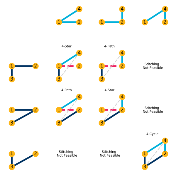
Figure 6: Stitchings of two-star graphlets with two common nodes

A more complicated example is provide by $\mathcal{W}_{2,\vbox{\hbox{\includegraphics[scale={0.125}]{twostar}}}}$ , which is shown in Figure 6. The format of the figure is the same as that of Figure 5. The two vertices in common are $1$ and $2$. An interesting feature of this example is that not all graphlet stitchings are feasible.

In evaluating $\Xi\left(\mathcal{W}_{q,S,R}\right)$ it is helpful to observe that $\mathcal{W}_{q,S,R}$ may include multiple isomorphisms of the same graph. Since the probabilities $\Pr\left(W=G_{N}\left[\left\{1,\ldots,p\right\}\right]\cup G_{N}\left[\left\{p-q,\ldots,2p-q\right\}\right]\right)$ and $\Pr\left(W^{\prime}=G_{N}\left[\left\{1,\ldots,p\right\}\right]\cup G_{N}\left[\left\{p-q,\ldots,2p-q\right\}\right]\right)$ coincide when $W$ and $W^{\prime}$ are isomorphic to one another, we can also “represent” $\mathcal{W}_{q,S,R}$ as a multi-set, with one (arbitrary) labelling of each of the non-isomorphic graphlet stitchings retained as elements, but with multiplicities equal to the number of isomorphic appearances. For example, the cardinality of $\mathcal{W}_{1,\vbox{\hbox{\includegraphics[scale={0.125}]{twostar}}}}$ is $\left|\mathrm{iso}\left(\vbox{\hbox{\includegraphics[scale={0.125}]{twostar}}}\right)\right|\times\left|\mathrm{iso}\left(\vbox{\hbox{\includegraphics[scale={0.125}]{twostar}}}\right)\right|=9$, but with only three non-isomorphic elements. Inspecting Figure 5 we define the multi-set:

$$\mathcal{W}_{1,\vbox{\hbox{\includegraphics[scale={0.125}]{twostar}}}}^{\mathrm{m}}=\left(\left\{\vbox{\hbox{\includegraphics[scale={0.125}]{fourstar}}},\vbox{\hbox{\includegraphics[scale={0.125}]{tailedthreestar}}},\vbox{\hbox{\includegraphics[scale={0.125}]{fivepath}}}\right\},\left\{\left(\vbox{\hbox{\includegraphics[scale={0.125}]{fourstar}}},1\right),\left(\vbox{\hbox{\includegraphics[scale={0.125}]{tailedthreestar}}},4\right),\left(\vbox{\hbox{\includegraphics[scale={0.125}]{fivepath}}},4\right)\right\}\right).$$

Let $\nu_{q,R,S}\left(W\right)$ denote the multiplicity of $W$ in $\mathcal{W}_{q,R,S}^{\mathrm{m}}$; for example the multiplicity of in $\mathcal{W}_{1,\vbox{\hbox{\includegraphics[scale={0.125}]{twostar}}}}^{\mathrm{m}}$ is $\nu_{1,\vbox{\hbox{\includegraphics[scale={0.125}]{twostar}}}}\left(\vbox{\hbox{\includegraphics[scale={0.125}]{tailedthreestar}}}\right)=4$.

We then have that, using equation (93), the equality $\Xi\left(\mathcal{W}_{1,\vbox{\hbox{\includegraphics[scale={0.125}]{twostar}}}}^{\mathrm{m}}\right)=\Xi\left(\mathcal{W}_{1,\vbox{\hbox{\includegraphics[scale={0.125}]{twostar}}}}\right)$. Similarly, inspecting $\mathcal{W}_{2,\vbox{\hbox{\includegraphics[scale={0.125}]{twostar}}}}$ (see Figure 6) , we see that it also contains three non-isomorphic elements, yielding

$$\mathcal{W}_{2,\vbox{\hbox{\includegraphics[scale={0.125}]{twostar}}}}^{\mathrm{m}}=\left(\left\{\vbox{\hbox{\includegraphics[scale={0.125}]{onethreewheel}}},\vbox{\hbox{\includegraphics[scale={0.125}]{fourpath}}},\vbox{\hbox{\includegraphics[scale={0.125}]{fourcycle}}}\right\},\left\{\left(\vbox{\hbox{\includegraphics[scale={0.125}]{onethreewheel}}},2\right),\left(\vbox{\hbox{\includegraphics[scale={0.125}]{fourpath}}},2\right),\left(\vbox{\hbox{\includegraphics[scale={0.125}]{fourcycle}}},1\right)\right\}\right).$$

Finally, it is easy to see that $\mathcal{W}_{3,\vbox{\hbox{\includegraphics[scale={0.125}]{twostar}}}}^{\mathrm{m}}=\left(\left\{\vbox{\hbox{\includegraphics[scale={0.125}]{twostar}}}\right\},\left\{\left(\vbox{\hbox{\includegraphics[scale={0.125}]{twostar}}},3\right)\right\}\right)$. The reader may verify that

$$\mathcal{W}_{1,\vbox{\hbox{\includegraphics[scale={0.125}]{triangle}}}}^{\mathrm{m}}=\left(\left\{\vbox{\hbox{\includegraphics[scale={0.125}]{twotriangle}}}\right\},\left\{\left(\vbox{\hbox{\includegraphics[scale={0.125}]{twotriangle}}},1\right)\right\}\right),\thinspace\mathcal{W}_{2,\vbox{\hbox{\includegraphics[scale={0.125}]{triangle}}}}^{\mathrm{m}}=\left(\left\{\vbox{\hbox{\includegraphics[scale={0.125}]{chordalcycle}}}\right\},\left\{\left(\vbox{\hbox{\includegraphics[scale={0.125}]{chordalcycle}}},1\right)\right\}\right),\thinspace\mathcal{W}_{3,\vbox{\hbox{\includegraphics[scale={0.125}]{triangle}}}}^{\mathrm{m}}=\left(\left\{\vbox{\hbox{\includegraphics[scale={0.125}]{triangle}}}\right\},\left\{\left(\vbox{\hbox{\includegraphics[scale={0.125}]{triangle}}},1\right)\right\}\right)$$

as well as that

$$\mathcal{W}_{1,\vbox{\hbox{\includegraphics[scale={0.125}]{twostar}}},\vbox{\hbox{\includegraphics[scale={0.125}]{triangle}}}}^{\mathrm{m}}=\left(\left\{\vbox{\hbox{\includegraphics[scale={0.125}]{twotailedtriangle}}},\vbox{\hbox{\includegraphics[scale={0.125}]{rattailedtriangle}}}\right\},\left\{\left(\vbox{\hbox{\includegraphics[scale={0.125}]{twotailedtriangle}}},1\right),\left(\vbox{\hbox{\includegraphics[scale={0.125}]{rattailedtriangle}}},2\right)\right\}\right),\thinspace\mathcal{W}_{2,\vbox{\hbox{\includegraphics[scale={0.125}]{twostar}}},\vbox{\hbox{\includegraphics[scale={0.125}]{triangle}}}}^{\mathrm{m}}=\left(\left\{\vbox{\hbox{\includegraphics[scale={0.125}]{tailedtriangle}}}\right\},\left\{\left(\vbox{\hbox{\includegraphics[scale={0.125}]{tailedtriangle}}},2\right)\right\}\right),\thinspace\mathcal{W}_{3,\vbox{\hbox{\includegraphics[scale={0.125}]{twostar}}},\vbox{\hbox{\includegraphics[scale={0.125}]{triangle}}}}^{\mathrm{m}}=\emptyset.$$

These multi-sets will be used to study the covariance of $\left(P_{N}\left(\vbox{\hbox{\includegraphics[scale={0.125}]{twostar}}}\right),P_{N}\left(\vbox{\hbox{\includegraphics[scale={0.125}]{triangle}}}\right)\right)^{\prime}$ as well as the variance of the transitivity index.

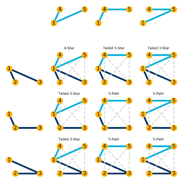
Figure 5: Stitchings of two-star graphlets with one common node

Notes: Depiction of all possible ways to join (or “stitch”) a pair of two-star ( ) subgraphs together with one node in common. Each of the resulting subgraphs is a pentad wiring. The dashed gray edges involve pairs of nodes that are not common across the pair of two-stars. Hence the subgraph induced by the five nodes in the pentad may or may not include these edges. The set $\mathcal{W}_{1,\vbox{\hbox{\includegraphics[scale={0.125}]{twostar}}}}$ has $\left|\mathrm{iso}\left(\vbox{\hbox{\includegraphics[scale={0.125}]{twostar}}}\right)\right|\times\left|\mathrm{iso}\left(\vbox{\hbox{\includegraphics[scale={0.125}]{twostar}}}\right)\right|=9$ elements.

Source: Author’s calculations.

At the risk of overkill, the following calculations illustrate how the two stitching probability definitions, equations (92) and (93), coincide. For the two-star example, starting with equation (92), I get

$$\Xi\left(\mathcal{W}_{1,\vbox{\hbox{\includegraphics[scale={0.125}]{twostar}}}}\right)= \frac{\Pr\left(\vbox{\hbox{\includegraphics[scale={0.125}]{twostar}}}\cong G_{N}\left[\left\{1,2,3\right\}\right]\thinspace\&\thinspace\vbox{\hbox{\includegraphics[scale={0.125}]{twostar}}}\cong G_{N}\left[\left\{1,4,5\right\}\right]\right)}{\left|\mathrm{iso}\left(\vbox{\hbox{\includegraphics[scale={0.125}]{twostar}}}\right)\right|^{2}}$$

$$= \frac{1}{\left|\mathrm{iso}\left(\vbox{\hbox{\includegraphics[scale={0.125}]{twostar}}}\right)\right|^{2}}\mathbb{E}\left[\left\{D_{12}D_{13}\left(1-D_{23}\right)+D_{12}\left(1-D_{13}\right)D_{23}+\left(1-D_{12}\right)D_{13}D_{23}\right\}\right.$$

$$\left.\times\left\{D_{14}D_{15}\left(1-D_{45}\right)+D_{14}\left(1-D_{15}\right)D_{45}+\left(1-D_{14}\right)D_{15}D_{45}\right\}\right]$$

$$= \frac{1}{\left|\mathrm{iso}\left(\vbox{\hbox{\includegraphics[scale={0.125}]{twostar}}}\right)\right|^{2}}\left\{\mathbb{E}\left[D_{12}D_{13}\left(1-D_{23}\right)D_{14}D_{15}\left(1-D_{45}\right)\right]\right|$$

$$+4\mathbb{E}\left[D_{12}D_{13}\left(1-D_{23}\right)D_{14}\left(1-D_{15}\right)D_{45}\right]$$

$$\left.+4\mathbb{E}\left[D_{12}\left(1-D_{13}\right)D_{23}D_{14}\left(1-D_{15}\right)D_{45}\right]\right\}$$

$$= \frac{1}{\left|\mathrm{iso}\left(\vbox{\hbox{\includegraphics[scale={0.125}]{twostar}}}\right)\right|^{2}}\left[\nu_{1,\vbox{\hbox{\includegraphics[scale={0.125}]{twostar}}}}\left(\vbox{\hbox{\includegraphics[scale={0.125}]{fourstar}}}\right)\Pr\left(\vbox{\hbox{\includegraphics[scale={0.125}]{fourstar}}}=G_{N}\left[\left\{1,2,3\right\}\right]\cup G_{N}\left[\left\{1,4,5\right\}\right]\right)\right.$$

$$+\nu_{1,\vbox{\hbox{\includegraphics[scale={0.125}]{twostar}}}}\left(\vbox{\hbox{\includegraphics[scale={0.125}]{tailedthreestar}}}\right)\Pr\left(\vbox{\hbox{\includegraphics[scale={0.125}]{tailedthreestar}}}=G_{N}\left[\left\{1,2,3\right\}\right]\cup G_{N}\left[\left\{1,4,5\right\}\right]\right)$$

$$\left.+\nu_{1,\vbox{\hbox{\includegraphics[scale={0.125}]{twostar}}}}\left(\vbox{\hbox{\includegraphics[scale={0.125}]{fivepath}}}\right)\Pr\left(\vbox{\hbox{\includegraphics[scale={0.125}]{fivepath}}}=G_{N}\left[\left\{1,2,3\right\}\right]\cup G_{N}\left[\left\{1,4,5\right\}\right]\right)\right]$$

$$= \sum_{W\in\mathcal{W}_{1,\vbox{\hbox{\includegraphics[scale={0.125}]{twostar}}}}^{\mathrm{m}}}\nu_{1,\vbox{\hbox{\includegraphics[scale={0.125}]{twostar}}}}\left(W\right)\Pr\left(W=G_{N}\left[\left\{1,2,3\right\}\right]\cup G_{N}\left[\left\{1,4,5\right\}\right]\right)$$

$$= \Xi\left(\mathcal{W}_{1,\vbox{\hbox{\includegraphics[scale={0.125}]{twostar}}}}^{\mathrm{m}}\right).$$ (94)

The third equality follows from relationships like $\mathbb{E}\left[D_{12}D_{13}\left(1-D_{23}\right)D_{14}\left(1-D_{15}\right)D_{45}\right]=\mathbb{E}\left[D_{12}D_{13}\left(1-D_{23}\right)\left(1-D_{14}\right)D_{15}D_{45}\right]$, which allow for the grouping together of terms. The balance of the equalities are consequences of the definitions given above.

Notes: Depiction of all possible ways to join (or “stitch”) a pair of two-star ( ) subgraphs together with two nodes in common. Each of the resulting subgraphs is a tetrad wiring. The dashed gray edges involve the pair of nodes that is not common across the pair of two-stars. Hence the subgraph induced by the four nodes in the tetrad may or may not include this edge.

Source: Author’s calculations.

Sampling variances

With the above notations in hand, I now calculate the sampling variances of $\hat{P}(\vbox{\hbox{\includegraphics[scale={0.125}]{twostar}}})$ and $P_{N}(\vbox{\hbox{\includegraphics[scale={0.125}]{triangle}}})$ as well as their covariance. Holland & Leinhardt, (1970, 1976) were the first to derive variance expressions for subgraph counts. The specific development presented here follows Bhattacharya & Bickel, (2015). A Hoeffding, (1948) variance-composition gives

$$\mathbb{V}\left(\left(\begin{array}[]{c}P_{N}\left(\vbox{\hbox{\includegraphics[scale={0.125}]{triangle}}}\right)\\ P_{N}\left(\vbox{\hbox{\includegraphics[scale={0.125}]{twostar}}}\right)\end{array}\right)\right)=\binom{N}{3}^{-2}\sum_{q=0}^{3}\binom{N}{3}\binom{3}{q}\binom{N-3}{3-q}\left(\begin{array}[]{cc}\Sigma_{q}\left(\vbox{\hbox{\includegraphics[scale={0.125}]{triangle}}}\right)&\Sigma_{q}\left(\vbox{\hbox{\includegraphics[scale={0.125}]{triangle}}},\vbox{\hbox{\includegraphics[scale={0.125}]{twostar}}}\right)\\ \Sigma_{q}\left(\vbox{\hbox{\includegraphics[scale={0.125}]{triangle}}},\vbox{\hbox{\includegraphics[scale={0.125}]{twostar}}}\right)&\Sigma_{q}\left(\vbox{\hbox{\includegraphics[scale={0.125}]{twostar}}}\right)\end{array}\right)$$

with $\Sigma_{q}\left(\vbox{\hbox{\includegraphics[scale={0.125}]{triangle}}}\right)$, $\Sigma_{q}\left(\vbox{\hbox{\includegraphics[scale={0.125}]{twostar}}}\right)$ and $\Sigma_{q}\left(\vbox{\hbox{\includegraphics[scale={0.125}]{triangle}}},\vbox{\hbox{\includegraphics[scale={0.125}]{twostar}}}\right)$ as defined by (91) above (using the shorthand $\Sigma_{q}\left(S,S\right)=\Sigma_{q}\left(S\right)$ etc). Using the fact that each of these variances and covariances is zero when $q=0$ and reorganizing terms gives

$$\mathbb{V}\left(\left(\begin{array}[]{c}P_{N}\left(\vbox{\hbox{\includegraphics[scale={0.125}]{triangle}}}\right)\\ P_{N}\left(\vbox{\hbox{\includegraphics[scale={0.125}]{twostar}}}\right)\end{array}\right)\right)= \binom{N}{3}^{-2}\sum_{q=1}^{3}\binom{N}{3}\binom{3}{q}\binom{N-3}{3-q}\left[\begin{array}[]{cc}\Xi\left(\mathcal{W}_{q,\vbox{\hbox{\includegraphics[scale={0.125}]{triangle}}}}\right)&\Xi\left(\mathcal{W}_{q,\vbox{\hbox{\includegraphics[scale={0.125}]{triangle}}},\vbox{\hbox{\includegraphics[scale={0.125}]{twostar}}}}\right)\\ \Xi\left(\mathcal{W}_{q,\vbox{\hbox{\includegraphics[scale={0.125}]{triangle}}},\vbox{\hbox{\includegraphics[scale={0.125}]{twostar}}}}\right)&\Xi\left(\mathcal{W}_{q,\vbox{\hbox{\includegraphics[scale={0.125}]{twostar}}}}\right)\end{array}\right]$$

$$-\left[1-\frac{\left(N-3\right)!^{2}}{N!\left(N-6\right)!}\right]\left[\begin{array}[]{cc}P\left(\vbox{\hbox{\includegraphics[scale={0.125}]{triangle}}}\right)^{2}&P\left(\vbox{\hbox{\includegraphics[scale={0.125}]{triangle}}}\right)P\left(\vbox{\hbox{\includegraphics[scale={0.125}]{twostar}}}\right)\\ P\left(\vbox{\hbox{\includegraphics[scale={0.125}]{triangle}}}\right)P\left(\vbox{\hbox{\includegraphics[scale={0.125}]{twostar}}}\right)&P\left(\vbox{\hbox{\includegraphics[scale={0.125}]{twostar}}}\right)^{2}\end{array}\right].$$

In what follows I assume that the network generating process is such that, for each $N$, $\Sigma_{q}\left(\vbox{\hbox{\includegraphics[scale={0.125}]{triangle}}}\right)$ and $\Sigma_{q}\left(\vbox{\hbox{\includegraphics[scale={0.125}]{twostar}}}\right)$ are not identically equal to zero for $q\geq 1$. This prevents $P_{N}\left(\vbox{\hbox{\includegraphics[scale={0.125}]{triangle}}}\right)$ and $P_{N}\left(\vbox{\hbox{\includegraphics[scale={0.125}]{twostar}}}\right)$ from exhibiting degenerate U-Statistic-like attributes (c.f., Graham,, 2017, Theorem 1). The restriction is a real one, ruling out the Erdös-Renyi case. Separate results for this special case are presented below.

As introduced earlier, in order to accommodate sequences of networks with varying degrees of sparsity, we can index the underlying population graphon by $N$, setting $h_{N}\left(u,v\right)=\rho_{N}w\left(u,v\right)$ with $w\left(u,v\right)=f_{\left.U_{i},U_{j}\right|D_{ij}}\left(\left.u,v\right|D_{ij}=1\right)$ and allowing $\rho_{N}\rightarrow 0$ as $N\rightarrow\infty$. Under such a sequence of GGPs $P\left(\vbox{\hbox{\includegraphics[scale={0.125}]{triangle}}}\right)$ and $P\left(\vbox{\hbox{\includegraphics[scale={0.125}]{twostar}}}\right)$ will tend to zero. In order to understand the properties of $P_{N}\left(\vbox{\hbox{\includegraphics[scale={0.125}]{triangle}}}\right)$ vis-a-vis $P\left(\vbox{\hbox{\includegraphics[scale={0.125}]{triangle}}}\right)$ we must normalize. It is natural to normalize according to the number edges in the subgraph under consideration.

Let $\tilde{P}\left(\vbox{\hbox{\includegraphics[scale={0.125}]{triangle}}}\right)=P\left(\vbox{\hbox{\includegraphics[scale={0.125}]{triangle}}}\right)/\rho_{N}^{3}$, $\tilde{P}\left(\vbox{\hbox{\includegraphics[scale={0.125}]{twostar}}}\right)=P\left(\vbox{\hbox{\includegraphics[scale={0.125}]{twostar}}}\right)/\rho_{N}^{2}$, $\tilde{P}_{N}\left(\vbox{\hbox{\includegraphics[scale={0.125}]{triangle}}}\right)=P_{N}\left(\vbox{\hbox{\includegraphics[scale={0.125}]{triangle}}}\right)/\rho_{N}^{3}$ and so on. So normalizing I get

$$\mathbb{V}\left(\left(\begin{array}[]{c}\tilde{P}_{N}\left(\vbox{\hbox{\includegraphics[scale={0.125}]{triangle}}}\right)\\ \tilde{P}_{N}\left(\vbox{\hbox{\includegraphics[scale={0.125}]{twostar}}}\right)\end{array}\right)\right)= \binom{N}{3}^{-2}\sum_{q=1}^{3}\binom{N}{3}\binom{3}{q}\binom{N-3}{3-q}\left[\begin{array}[]{cc}\rho_{N}^{-6}\Xi\left(\mathcal{W}_{q,\vbox{\hbox{\includegraphics[scale={0.125}]{triangle}}}}\right)&\rho_{N}^{-5}\Xi\left(\mathcal{W}_{q,\vbox{\hbox{\includegraphics[scale={0.125}]{triangle}}},\vbox{\hbox{\includegraphics[scale={0.125}]{twostar}}}}\right)\\ \rho_{N}^{-5}\Xi\left(\mathcal{W}_{q,\vbox{\hbox{\includegraphics[scale={0.125}]{triangle}}},\vbox{\hbox{\includegraphics[scale={0.125}]{twostar}}}}\right)&\rho_{N}^{-4}\Xi\left(\mathcal{W}_{q,\vbox{\hbox{\includegraphics[scale={0.125}]{twostar}}}}\right)\end{array}\right]$$ (99)

$$-\left[1-\frac{\left(N-3\right)!^{2}}{N!\left(N-6\right)!}\right]\left[\begin{array}[]{cc}\tilde{P}\left(\vbox{\hbox{\includegraphics[scale={0.125}]{triangle}}}\right)^{2}&\tilde{P}\left(\vbox{\hbox{\includegraphics[scale={0.125}]{triangle}}}\right)\tilde{P}\left(\vbox{\hbox{\includegraphics[scale={0.125}]{twostar}}}\right)\\ \tilde{P}\left(\vbox{\hbox{\includegraphics[scale={0.125}]{triangle}}}\right)\tilde{P}\left(\vbox{\hbox{\includegraphics[scale={0.125}]{twostar}}}\right)&\tilde{P}\left(\vbox{\hbox{\includegraphics[scale={0.125}]{twostar}}}\right)^{2}\end{array}\right].$$ (102)

Expression (102) agrees with the corresponding expression of Bhattacharya & Bickel, (2015) for injective homomorphism frequencies (Equation (3.8), p. 2395). The main difference is the analog of $\Xi\left(\mathcal{W}_{q,\vbox{\hbox{\includegraphics[scale={0.125}]{triangle}}}}\right)$ in their expression is itself an injective homomorphism density, whereas here $\Xi\left(\mathcal{W}_{q,\vbox{\hbox{\includegraphics[scale={0.125}]{triangle}}}}\right)$ is neither an injective homomorphism nor an induced subgraph density and instead involves checking for particular patterns of both adjacency and non-adjacency as described above.

Rates of convergence

To understand the rate of convergence in mean square of, for example, $\tilde{P}_{N}\left(\vbox{\hbox{\includegraphics[scale={0.125}]{triangle}}}\right)$ toward $\tilde{P}\left(\vbox{\hbox{\includegraphics[scale={0.125}]{triangle}}}\right)$, we need to determine the order of each of the terms in (102). Let $e\left(R\right)\overset{def}{\equiv}\left|\mathcal{E}\left(R\right)\right|$ and $e\left(S\right)\overset{def}{\equiv}\left|\mathcal{E}\left(S\right)\right|$ denote the number of edges in graphlets $R$ and $S$. Next observe that $\binom{N}{p}^{-1}\binom{p}{q}\binom{N-p}{p-q}=O\left(N^{-q}\right)$. We therefore have that the terms in the summation indexed by $q$ in (102) are $O\left(N^{-q}\rho_{N}^{-e\left(R\right)}\rho_{N}^{-e\left(S\right)}\right)O\left(\Xi\left(\mathcal{W}_{q,R,S}\right)\right)$ for $q=1,\ldots,p.$ I divide these terms, closely following Bhattacharya & Bickel, (2015), into three cases:

Case 1 ($q=1$): when $q=1$ the number of edges in all elements of $\mathcal{W}_{q,R,S}$ equals $e\left(R\right)+e\left(S\right)$ for any subgraphs $R$ and $S$. Hence $O\left(\Xi\left(\mathcal{W}_{1,R,S}\right)\right)=O\left(\rho_{N}^{e\left(R\right)}\rho_{N}^{e\left(S\right)}\right)$, yielding

$$O\left(N^{-1}\rho_{N}^{-e\left(R\right)}\rho_{N}^{-e\left(S\right)}\right)O\left(\Xi\left(\mathcal{W}_{1,R,S}\right)\right)=O\left(N^{-1}\right).$$

The $q=1$ summand in (102) is of order $N^{-1}$. In general, from the theory of U-statistics, one would expect this to be the leading variance term; however, the present situation is more complicated.

Case 2 ($q=3$ or $q=p$): In this case the order of $\Xi\left(\mathcal{W}_{3,\vbox{\hbox{\includegraphics[scale={0.125}]{triangle}}}}\right)$ is $O\left(\rho_{N}^{3}\right)$, $\Xi\left(\mathcal{W}_{3,\vbox{\hbox{\includegraphics[scale={0.125}]{twostar}}}}\right)$ is $O\left(\rho_{N}^{2}\right)$ and $\mathcal{W}_{3,\vbox{\hbox{\includegraphics[scale={0.125}]{triangle}}},\vbox{\hbox{\includegraphics[scale={0.125}]{twostar}}}}$ is empty so that $\Xi\left(\text{$\mathcal{W}_{3,\vbox{\hbox{\includegraphics[scale={0.125}]{triangle}}},\vbox{\hbox{\includegraphics[scale={0.125}]{twostar}}}}$}\right)=0$. Therefore, recalling that $\lambda_{N}=\left(N-1\right)\rho_{N}$ equals average degree,

$$O\left(N^{-3}\rho_{N}^{-2e\left(\vbox{\hbox{\includegraphics[scale={0.125}]{triangle}}}\right)}\right)O\left(\Xi\left(\mathcal{W}_{3,\vbox{\hbox{\includegraphics[scale={0.125}]{triangle}}}}\right)\right) =O\left(\lambda_{N}^{-3}\right)$$

$$O\left(N^{-3}\rho_{N}^{-2e\left(\vbox{\hbox{\includegraphics[scale={0.125}]{twostar}}}\right)}\right)O\left(\Xi\left(\mathcal{W}_{3,\vbox{\hbox{\includegraphics[scale={0.125}]{twostar}}}}\right)\right) =O\left(N^{-1}\lambda_{N}^{-2}\right)$$

$$O\left(N^{-3}\rho_{N}^{-e\left(\vbox{\hbox{\includegraphics[scale={0.125}]{triangle}}}\right)}\rho_{N}^{-e\left(\vbox{\hbox{\includegraphics[scale={0.125}]{twostar}}}\right)}\right)O\left(\Xi\left(\mathcal{W}_{3,\vbox{\hbox{\includegraphics[scale={0.125}]{triangle}}},\vbox{\hbox{\includegraphics[scale={0.125}]{twostar}}}}\right)\right) =o\left(1\right).$$

Case 3 ($q=2$ or $\left(2\leq q\leq p-1\right)$): Here the order of $\Xi\left(\mathcal{W}_{2,\vbox{\hbox{\includegraphics[scale={0.125}]{triangle}}}}\right)$ equals $O\left(\rho_{N}^{2e\left(\vbox{\hbox{\includegraphics[scale={0.125}]{triangle}}}\right)-\left(q-1\right)}\right)=O\left(\rho_{N}^{5}\right)$, $\Xi\left(\mathcal{W}_{2,\vbox{\hbox{\includegraphics[scale={0.125}]{twostar}}}}\right)$ equals $O\left(\rho_{N}^{2e\left(\vbox{\hbox{\includegraphics[scale={0.125}]{twostar}}}\right)-\left(q-1\right)}\right)=O\left(\rho_{N}^{3}\right)$ and that of $\Xi\left(\text{$\mathcal{W}_{2,\vbox{\hbox{\includegraphics[scale={0.125}]{triangle}}},\vbox{\hbox{\includegraphics[scale={0.125}]{twostar}}}}$}\right)$ equals $O\left(\rho_{N}^{e\left(\vbox{\hbox{\includegraphics[scale={0.125}]{triangle}}}\right)+e\left(\vbox{\hbox{\includegraphics[scale={0.125}]{twostar}}}\right)-\left(q-1\right)}\right)=O\left(\rho_{N}^{4}\right)$ . Therefore

$$O\left(N^{-2}\rho_{N}^{-2e\left(\vbox{\hbox{\includegraphics[scale={0.125}]{triangle}}}\right)}\right)O\left(\Xi\left(\mathcal{W}_{2,\vbox{\hbox{\includegraphics[scale={0.125}]{triangle}}}}\right)\right) =O\left(N^{-1}\lambda_{N}^{-1}\right)$$

$$O\left(N^{-2}\rho_{N}^{-2e\left(\vbox{\hbox{\includegraphics[scale={0.125}]{twostar}}}\right)}\right)O\left(\Xi\left(\mathcal{W}_{2,\vbox{\hbox{\includegraphics[scale={0.125}]{twostar}}}}\right)\right) =O\left(N^{-1}\lambda_{N}^{-1}\right)$$

$$O\left(N^{-2}\rho_{N}^{-e\left(\vbox{\hbox{\includegraphics[scale={0.125}]{triangle}}}\right)}\rho_{N}^{-e\left(\vbox{\hbox{\includegraphics[scale={0.125}]{twostar}}}\right)}\right)O\left(\Xi\left(\mathcal{W}_{2,\vbox{\hbox{\includegraphics[scale={0.125}]{triangle}}},\vbox{\hbox{\includegraphics[scale={0.125}]{twostar}}}}\right)\right) =O\left(N^{-1}\lambda_{N}^{-1}\right).$$

For the two variance terms we have

$$\mathbb{V}\left(\tilde{P}_{N}\left(\vbox{\hbox{\includegraphics[scale={0.125}]{triangle}}}\right)\right) =O\left(\frac{1}{N}\right)+O\left(\frac{1}{N\lambda_{N}}\right)+O\left(\frac{1}{\lambda_{N}^{3}}\right)$$

$$\mathbb{V}\left(\tilde{P}_{N}\left(\vbox{\hbox{\includegraphics[scale={0.125}]{twostar}}}\right)\right) =O\left(\frac{1}{N}\right)+O\left(\frac{1}{N\lambda_{N}}\right)+O\left(\frac{1}{N\lambda_{N}^{2}}\right)$$

indicating that the rate at which, for example, $\tilde{P}_{N}\left(\vbox{\hbox{\includegraphics[scale={0.125}]{triangle}}}\right)$ converges in mean square toward $\tilde{P}\left(\vbox{\hbox{\includegraphics[scale={0.125}]{triangle}}}\right)$, depends on the behavior of average degree as the network grows large. This reflects the fact that, depending on a combination of the nature of the graphlet of interest and the rate at which $\lambda_{N}$ does, or does not, grows with $N$, several of the terms in (102) may be of equal order.

For any increasing sequence of average degree we have

$$\mathbb{V}\left(\tilde{P}_{N}\left(\vbox{\hbox{\includegraphics[scale={0.125}]{triangle}}}\right)\right)= O\left(\max\left(\frac{1}{N},\frac{1}{\lambda_{N}^{3}}\right)\right)$$

$$\mathbb{V}\left(\tilde{P}_{N}\left(\vbox{\hbox{\includegraphics[scale={0.125}]{twostar}}}\right)\right)= O\left(\frac{1}{N}\right)$$

$$\mathbb{C}\left(\tilde{P}_{N}\left(\vbox{\hbox{\includegraphics[scale={0.125}]{triangle}}}\right),\tilde{P}_{N}\left(\vbox{\hbox{\includegraphics[scale={0.125}]{twostar}}}\right)\right)= O\left(\frac{1}{N}\right).$$

If $\lambda_{N}\geq CN^{1/3}$, then the rate of convergence is $\sqrt{N}$ for both $\tilde{P}_{N}\left(\vbox{\hbox{\includegraphics[scale={0.125}]{twostar}}}\right)$ and $\tilde{P}_{N}\left(\vbox{\hbox{\includegraphics[scale={0.125}]{triangle}}}\right)$. In the sparse case, with $\lambda_{N}\rightarrow\lambda$, $\tilde{P}\left(\vbox{\hbox{\includegraphics[scale={0.125}]{twostar}}}\right)$, due to the acyclic structure of the two-star graphlet, remains estimable at the $\sqrt{N}$ rate. However in this case all three of its variance terms are of equal order. In contrast $\tilde{P}\left(\vbox{\hbox{\includegraphics[scale={0.125}]{triangle}}}\right)$ is (evidently) not consistently estimable in the sparse case.

Asymptotic normality

When average degree is $\lambda_{N}>CN^{1/3}$, such that both $\tilde{P}_{N}\left(\vbox{\hbox{\includegraphics[scale={0.125}]{twostar}}}\right)$ and $\tilde{P}_{N}\left(\vbox{\hbox{\includegraphics[scale={0.125}]{triangle}}}\right)$ converge at the $\sqrt{N}$ rate, an application of Theorem 1.c of Bickel et al., (2011) establishes that, under some regularity conditions,

$$\sqrt{N}\left(\begin{array}[]{c}\tilde{P}_{N}\left(\vbox{\hbox{\includegraphics[scale={0.125}]{triangle}}}\right)-\tilde{P}\left(\vbox{\hbox{\includegraphics[scale={0.125}]{triangle}}}\right)\\ \tilde{P}_{N}\left(\vbox{\hbox{\includegraphics[scale={0.125}]{twostar}}}\right)-\tilde{P}\left(\vbox{\hbox{\includegraphics[scale={0.125}]{twostar}}}\right)\end{array}\right)\overset{D}{\rightarrow}\mathcal{N}\left(\left(\begin{array}[]{c}0\\ 0\end{array}\right),9\left(\begin{array}[]{cc}\tilde{\Sigma}_{1}\left(\vbox{\hbox{\includegraphics[scale={0.125}]{triangle}}}\right)&\tilde{\Sigma}_{1}\left(\vbox{\hbox{\includegraphics[scale={0.125}]{triangle}}},\vbox{\hbox{\includegraphics[scale={0.125}]{twostar}}}\right)\\ \tilde{\Sigma}_{1}\left(\vbox{\hbox{\includegraphics[scale={0.125}]{triangle}}},\vbox{\hbox{\includegraphics[scale={0.125}]{twostar}}}\right)&\tilde{\Sigma}_{1}\left(\vbox{\hbox{\includegraphics[scale={0.125}]{twostar}}}\right)\end{array}\right)\right),$$ (103)

where $\tilde{\Sigma}_{1}\left(\vbox{\hbox{\includegraphics[scale={0.125}]{triangle}}}\right)=\rho_{N}^{-6}\Sigma_{1}\left(\vbox{\hbox{\includegraphics[scale={0.125}]{triangle}}}\right)$, $\tilde{\Sigma}_{1}\left(\vbox{\hbox{\includegraphics[scale={0.125}]{triangle}}},\vbox{\hbox{\includegraphics[scale={0.125}]{twostar}}}\right)=\rho_{N}^{-5}\Sigma_{1}\left(\vbox{\hbox{\includegraphics[scale={0.125}]{triangle}}},\vbox{\hbox{\includegraphics[scale={0.125}]{twostar}}}\right)$ etc. Proving (103) is relatively straightforward. I do not sketch the argument here, but note that the main tools needed were already introduced in the analysis of dyadic regression appearing in Section 4 above.

As noted previously, if $\lambda_{N}\rightarrow\lambda$ as $N\rightarrow\infty$ such that the network is sparse in the limit, then a general result on $\sqrt{N}\left(\tilde{P}_{N}\left(\vbox{\hbox{\includegraphics[scale={0.125}]{triangle}}}\right)-\tilde{P}\left(\vbox{\hbox{\includegraphics[scale={0.125}]{triangle}}}\right)\right)$ is unavailable. In contrast, part (b) of Theorem 1 in Bickel et al., (2011) implies that not only does $\tilde{P}_{N}\left(\vbox{\hbox{\includegraphics[scale={0.125}]{twostar}}}\right)$ remain $\sqrt{N}$ consistent for $\tilde{P}\left(\vbox{\hbox{\includegraphics[scale={0.125}]{twostar}}}\right)$ in this case, but also that $\sqrt{N}\left(\tilde{P}_{N}\left(\vbox{\hbox{\includegraphics[scale={0.125}]{twostar}}}\right)-\tilde{P}\left(\vbox{\hbox{\includegraphics[scale={0.125}]{twostar}}}\right)\right)$ remains asymptotically normal. The limiting variance in this case differs from the one given in (103); all terms in $\mathbb{V}\left(\tilde{P}_{N}\left(\vbox{\hbox{\includegraphics[scale={0.125}]{twostar}}}\right)\right)$ are of equal order (and hence should be retained).

More generally the sampling properties of induced subgraph frequencies under sparse graph limits remains relatively unexplored. The sensitivity of rates of convergence and distributional properties to assumptions about $\lambda_{N}$ raises concerns about uniformity of inference procedures. A similar concern is suggested by the properties of these statistics when the graphon is constant. This last case is considered next.

Two-star and triangle counts in Erdös-Renyi networks

The analysis above assumes that the graphon is such that $\mathbb{C}\left(\mathbf{1}\left(R\cong G_{N}\left[\mathbf{i}_{p}\right]\right),\mathbf{1}\left(S\cong G_{N}\left[\mathbf{j}_{p}\right]\right)\right)\neq 0$ when $\mathbf{i}_{p}$ and $\mathbf{j}_{p}$ share exactly one index in common (such that $\Xi\left(\mathcal{W}_{1,S}\right)-P\left(S\right)^{2}>0$). This condition will generally hold for graphons which vary in $u$ and $v$ (such that the events $D_{12}=1$ and $D_{13}=1$ are not independent), but it does rule out the Erdös-Renyi case (where links form independently with constant probability $\rho$). This graph generation process has been extensively studied by probabilists for over sixty years (e.g., Janson et al.,, 2000).

In statistics, Janson & Nowicki, (1991) and Nowicki, (1991) studied the sampling properties of induced and partial subgraph frequencies when the network is an Erdös-Renyi one. They demonstrated asymptotic normality of such frequencies with a $\sqrt{\tbinom{N}{2}}$ rate of convergence. These earlier results, at first glance, appear to be in tension with the more general results of Bickel et al., (2011), who showed asymptotic normality with a $\sqrt{N}$ rate of convergence under general graphons. It turns out, however, that the leading (i.e., $q=1$) term in (102) is identically equal to zero under the Erdös-Renyi GPP. The Erdös-Renyi GPP is a “degenerate” special case.

To see this, evaluate the stitching probabilities (93) under the Erdös-Renyi GPP to get

$$\Xi\left(\mathcal{W}_{1,\vbox{\hbox{\includegraphics[scale={0.125}]{twostar}}}}\right)=\rho^{4}\left(1-\rho\right)^{2},\thinspace\Xi\left(\mathcal{W}_{2,\vbox{\hbox{\includegraphics[scale={0.125}]{twostar}}}}\right)=\frac{4}{9}\rho^{3}\left(1-\rho\right)^{2}+\frac{1}{9}\rho^{4}\left(1-\rho\right),\thinspace\Xi\left(\mathcal{W}_{3,\vbox{\hbox{\includegraphics[scale={0.125}]{twostar}}}}\right)=\frac{1}{3}\rho^{2}\left(1-\rho\right)$$

and

$$\Xi\left(\mathcal{W}_{1,\vbox{\hbox{\includegraphics[scale={0.125}]{triangle}}}}\right)=\rho^{6},\thinspace\Xi\left(\mathcal{W}_{2,\vbox{\hbox{\includegraphics[scale={0.125}]{triangle}}}}\right)=\rho^{5},\thinspace\Xi\left(\mathcal{W}_{3,\vbox{\hbox{\includegraphics[scale={0.125}]{triangle}}}}\right)=\rho^{3}$$

and

$$\Xi\left(\mathcal{W}_{1,\vbox{\hbox{\includegraphics[scale={0.125}]{twostar}}},\vbox{\hbox{\includegraphics[scale={0.125}]{triangle}}}}\right)=\rho^{5}\left(1-\rho\right),\thinspace\Xi\left(\mathcal{W}_{2,\vbox{\hbox{\includegraphics[scale={0.125}]{twostar}}},\vbox{\hbox{\includegraphics[scale={0.125}]{triangle}}}}\right)=\frac{2}{3}\rho^{4}\left(1-\rho\right),\thinspace\Xi\left(\mathcal{W}_{3,\vbox{\hbox{\includegraphics[scale={0.125}]{twostar}}},\vbox{\hbox{\includegraphics[scale={0.125}]{triangle}}}}\right)=0.$$

Under these graphlet stitching probabilities the $q=1$ variance term, which is generally the leading variance term in Bickel et al., (2011, Theorem 1), instead equals

$$\left(\begin{array}[]{cc}\Sigma_{1}\left(\vbox{\hbox{\includegraphics[scale={0.125}]{triangle}}}\right)&\Sigma_{1}\left(\vbox{\hbox{\includegraphics[scale={0.125}]{triangle}}},\vbox{\hbox{\includegraphics[scale={0.125}]{twostar}}}\right)\\ \Sigma_{1}\left(\vbox{\hbox{\includegraphics[scale={0.125}]{triangle}}},\vbox{\hbox{\includegraphics[scale={0.125}]{twostar}}}\right)&\Sigma_{1}\left(\vbox{\hbox{\includegraphics[scale={0.125}]{twostar}}}\right)\end{array}\right)=\mathbf{0}_{2}\mathbf{0}_{2}^{\prime}.$$

Hence, under the (dense) Erdös-Renyi GPP, the leading variance term is instead the $q=2$ one, yielding for $0<\rho<1$ but $\rho\neq 2/3$,

$$\sqrt{\tbinom{N}{2}}\left(\begin{array}[]{c}P_{N}\left(\vbox{\hbox{\includegraphics[scale={0.125}]{triangle}}}\right)-P\left(\vbox{\hbox{\includegraphics[scale={0.125}]{triangle}}}\right)\\ P_{N}\left(\vbox{\hbox{\includegraphics[scale={0.125}]{twostar}}}\right)-P\left(\vbox{\hbox{\includegraphics[scale={0.125}]{twostar}}}\right)\end{array}\right) \overset{D}{\rightarrow}\mathcal{N}\left(\left(\begin{array}[]{c}0\\ 0\end{array}\right),9\left(\begin{array}[]{cc}\Sigma_{2}\left(\vbox{\hbox{\includegraphics[scale={0.125}]{triangle}}}\right)&\Sigma_{2}\left(\vbox{\hbox{\includegraphics[scale={0.125}]{triangle}}},\vbox{\hbox{\includegraphics[scale={0.125}]{twostar}}}\right)\\ \Sigma_{2}\left(\vbox{\hbox{\includegraphics[scale={0.125}]{triangle}}},\vbox{\hbox{\includegraphics[scale={0.125}]{twostar}}}\right)&\Sigma_{2}\left(\vbox{\hbox{\includegraphics[scale={0.125}]{twostar}}}\right)\end{array}\right)\right)$$ (110)

where

$$\left(\begin{array}[]{cc}\Sigma_{2}\left(\vbox{\hbox{\includegraphics[scale={0.125}]{triangle}}}\right)&\Sigma_{2}\left(\vbox{\hbox{\includegraphics[scale={0.125}]{triangle}}},\vbox{\hbox{\includegraphics[scale={0.125}]{twostar}}}\right)\\ \Sigma_{2}\left(\vbox{\hbox{\includegraphics[scale={0.125}]{triangle}}},\vbox{\hbox{\includegraphics[scale={0.125}]{twostar}}}\right)&\Sigma_{2}\left(\vbox{\hbox{\includegraphics[scale={0.125}]{twostar}}}\right)\end{array}\right)=\rho^{3}\left(1-\rho\right)\left(\begin{array}[]{cc}\rho^{2}&\frac{1}{3}\rho\left(2-3\rho\right)\\ \frac{1}{3}\rho\left(2-3\rho\right)&\frac{1}{9}\left(2-3\rho\right)^{2}\end{array}\right).$$

See Corollaries 2 and 4 of Nowicki, (1991) for additional context and references to the primary literature.

Uniform Inference

The analysis of the previous two subsections showed how the limiting distributions of two-star and triangle frequencies are sensitive to the form of the graphon, $h_{N}\left(u,v\right)=\rho_{N}w\left(u,v\right)$. If $\rho_{N}$ approaches zero too quickly, or $w\left(u,v\right)$ is a constant, the rate of convergence of the estimator changes. This raises concerns about how to conduct inference in settings where the limiting graph is ‘close to sparse’ and/or the graphon is ‘nearly’ constant, or equivalently, dependence across dyads sharing agents in common is weak. In such settings an approach to inference based on (103), may have poor properties when $N$ is finite. This is because the $q=1$, $q=2$ and $q=3$ terms in the variance expression (102) may all be of similar order. For this reason, it seems advisable to keep all terms when calculating variances for test statistics. Clearly, there are open questions on how best to undertake testing in this setting.

Application of results to inference on transitivity in Nyakatoke

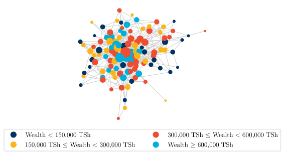
Figure 7: Nyakatoke risk-sharing network

Sources: De Weerdt, (2004) and authors’ calculations. ‘TSh’ is an abbreviation for Tanzanian Shillings.

De Weerdt, (2004) collected information of risk-sharing relationships across 119 houses in Nyakatoke, a small village in Tanzania (see Figure 8). The density of this network is 0.0698, while its transitivity index is 0.1884, nearly three times a large. A natural question is whether the high transitivity index simple reflects “chance” or is a real feature of Nyakatoke. To assess this I construct a confidence interval for the transitivity index using the delta method and the results outlined above. Other than the empirical illustration included in Bhattacharya & Bickel, (2015), I am aware of no other published examples of large network inference on the transitivity index.

The natural analog estimates of $\Xi\left(\mathcal{W}_{1,\vbox{\hbox{\includegraphics[scale={0.125}]{triangle}}}}\right)$, $\Xi\left(\mathcal{W}_{1,\vbox{\hbox{\includegraphics[scale={0.125}]{twostar}}}}\right)$, and $\Xi\left(\mathcal{W}_{1,\vbox{\hbox{\includegraphics[scale={0.125}]{triangle}}},\vbox{\hbox{\includegraphics[scale={0.125}]{twostar}}}}\right)$ involve summations over all $\tbinom{N}{3}\tbinom{3}{1}\tbinom{N-3}{3-1}=30\times\tbinom{N}{5}$ pairs of triads sharing exactly one common agent. This requires evaluating the configuration of all $\tbinom{N}{5}$ pentads in the network; a computationally non-trivial task even for medium-sized networks. It is for this reason that Bhattacharya & Bickel, (2015) suggest a subsampling approach to variance estimation.

For the Nyakatoke network we have a total of $\binom{119}{3}=273,819$ triad configurations to count and a total of $\binom{119}{5}=182,637,273$ pentads that need to be inspected in order to calculate variances. These are large numbers, but nevertheless small enough enough for a desktop computer to handle in a few minutes. Direct calculation gives

$$P_{N}\left(\vbox{\hbox{\includegraphics[scale={0.125}]{triangle}}}\right)=\begin{array}[]{c}0.00115\\ (0.00030)\end{array},\thinspace\thinspace P_{N}\left(\vbox{\hbox{\includegraphics[scale={0.125}]{twostar}}}\right)=\begin{array}[]{c}0.00496\\ (0.00100)\end{array}$$

These standard errors include estimates of both the first and last terms in (102) above, although the second of these is asymptotically negligible as long as average degree grows fast enough (which is assumed for the asymptotic normality result).

Applying the delta method I get an estimated standard error for the transitivity index of 0.011; this suggests that transitivity is significantly greater than what we would expect to observe under the Erdös-Renyi random graph null.

7.2 Moments of the degree distribution

Networks are complex objects, making their analysis both conceptually and technically challenging. One approach to simplification involves looking only at the number of links each agent has, that is their degree, $D_{i+}=\sum_{j\neq i}D_{ij}$, ignoring all other architectural features of the network. Indeed, a substantial empirical literature focuses on the degree sequence of a network as its primary object of interest (Barabási & Albert,, 1999; Barabási,, 2016).

Most real world networks exhibit substantial degree heterogeneity, making the degree sequence an interesting statistic to study and model. A network’s degree sequence is also straightforward to measure. A researcher need only ask about the number of friends, suppliers, or partners each agent has, not their identity. Many general purpose datasets collect such information. For example General Social Survey (GSS) sometimes collects information on the number of close confidants (cf., Marsden,, 1987; McPherson et al.,, 2006), while demographers routinely collect information on the number of lifetime and/or concurrent sexual partners. Simplicity and data availability both drive the substantial focus on degree distributions in empirical work.

It is possible for two graphs with the same degree sequence to be topologically different; their diameters and transitivity indices, for example, may differ substantially. At the same time a network’s degree sequence is an important summary statistic, constraining other features of it, even local ones. This is shown by Theorem 3, which I believe is an original result (albeit perhaps folk wisdom; Snijders et al.,, 2006, cf., ).

Theorem 3.

(Degree Sequence Moments) Let $G$ be an exchangeable random graph of order $N$. The $m^{th}$ moment of $D_{i+}=\sum_{j\neq i}D_{ij}$ equals

$$\mathbb{E}\left[D_{i+}^{m}\right] =\sum_{k=1}^{m}C_{k,m}\times\mathbb{E}\left[D_{ij_{1}}\times\cdots\times D_{ij_{k}}\right]$$

for $m=1,2,\ldots,N-1$ and $C_{k,m}=\tbinom{N-1}{k}\left(\sum_{\mathbf{p}\in\mathcal{P}_{k,m}}\frac{m!}{p_{1}!\times\cdots\times p_{k}!}\right)$ with

$$\mathcal{P}_{k,m}=\left\{\left(p_{1},\ldots,p_{k}\right)\thinspace:\thinspace\sum_{j=1}^{k}p_{j}=m,\thinspace p_{j}\in\mathbb{N}\text{ for $j=1,\ldots,k$}\right\}$$

and $\mathbb{N}$ the set of positive integers.

Proof.

See Appendix A. ∎

Theorem 3 implies that the first four uncentered moments of $D_{i+}$ equal

$$\mathbb{E}\left[D_{i+}\right]= \left(N-1\right)P\left(\vbox{\hbox{\includegraphics[scale={0.125}]{edge}}}\right)$$ (111)

$$\mathbb{E}\left[D_{i+}^{2}\right]= \left(N-1\right)P\left(\vbox{\hbox{\includegraphics[scale={0.125}]{edge}}}\right)+\left(N-1\right)\left(N-2\right)Q\left(\vbox{\hbox{\includegraphics[scale={0.125}]{twostar}}}\right)$$ (112)

$$\mathbb{E}\left[D_{i+}^{3}\right]= \left(N-1\right)P\left(\vbox{\hbox{\includegraphics[scale={0.125}]{edge}}}\right)+3\left(N-1\right)\left(N-2\right)Q\left(\vbox{\hbox{\includegraphics[scale={0.125}]{twostar}}}\right)$$ (113)

$$+\left(N-1\right)\left(N-2\right)\left(N-3\right)Q\left(\vbox{\hbox{\includegraphics[scale={0.125}]{onethreewheel}}}\right)$$

$$\mathbb{E}\left[D_{i+}^{4}\right]= \left(N-1\right)P\left(\vbox{\hbox{\includegraphics[scale={0.125}]{edge}}}\right)+7\left(N-1\right)\left(N-2\right)Q\left(\vbox{\hbox{\includegraphics[scale={0.125}]{twostar}}}\right)$$ (114)

$$+6\left(N-1\right)\left(N-2\right)\left(N-3\right)Q\left(\vbox{\hbox{\includegraphics[scale={0.125}]{onethreewheel}}}\right)$$

$$+\left(N-1\right)\left(N-2\right)\left(N-3\right)\left(N-4\right)Q\left(\vbox{\hbox{\includegraphics[scale={0.125}]{fourstar}}}\right).$$

In dense networks it is natural to divide $D_{i+}$ by $N-1$. With degrees so normalized, all terms in equations (111) to (114) are asymptotically dominated by the last one as $N\rightarrow\infty$. Hence, in the limit, the $k^{th}$ moment of normalized degree equals the injective homomorphism density of $k$-stars in the limiting graphon (cf., Diaconis et al.,, 2008, Lemma 4.1). In the dense case we have, for example, that

$$\underset{N\rightarrow\infty}{\lim}\mathbb{V}\left(\frac{D_{i+}}{N-1}\right)=Q\left(\vbox{\hbox{\includegraphics[scale={0.125}]{twostar}}}\right)-P\left(\vbox{\hbox{\includegraphics[scale={0.125}]{edge}}}\right)P\left(\vbox{\hbox{\includegraphics[scale={0.125}]{edge}}}\right).$$ (115)

When the network is not dense, the natural normalization is instead by average degree, $\lambda_{N}=\left(N-1\right)\rho_{N}$, which may no longer be proportional to $N$ in the limit. In the sparse case, $\lambda_{N}\rightarrow\lambda$, and all terms in equations (111) to (114) are of equal order. For example, the fourth uncentered moment of $D_{i+}/\lambda_{N}$ equals, in a sparse limit,

$$\underset{N\rightarrow\infty}{\lim}\mathbb{E}\left[\left(\frac{D_{i+}}{\lambda_{N}}\right)^{4}\right]=\frac{\tilde{P}\left(\vbox{\hbox{\includegraphics[scale={0.125}]{edge}}}\right)}{\lambda^{3}}+\frac{7\tilde{Q}\left(\vbox{\hbox{\includegraphics[scale={0.125}]{twostar}}}\right)}{\lambda^{2}}+\frac{6\tilde{Q}\left(\vbox{\hbox{\includegraphics[scale={0.125}]{onethreewheel}}}\right)}{\lambda}+\tilde{Q}\left(\vbox{\hbox{\includegraphics[scale={0.125}]{fourstar}}}\right),$$

where a tilde above a subgraph/homomorphism density, as earlier, denotes the density divided by $\rho_{N}$ raised to the power of the number of edges in the subgraph under consideration (e.g., $\tilde{Q}\left(\vbox{\hbox{\includegraphics[scale={0.125}]{twostar}}}\right)=Q\left(\vbox{\hbox{\includegraphics[scale={0.125}]{twostar}}}\right)/\rho_{N}^{2}$).

From (111) and (112) have that, in the sparse case,

$$\underset{N\rightarrow\infty}{\lim}\mathbb{V}\left(\frac{D_{i+}}{\lambda_{N}}\right)=\left[\tilde{Q}\left(\vbox{\hbox{\includegraphics[scale={0.125}]{twostar}}}\right)-\tilde{P}\left(\vbox{\hbox{\includegraphics[scale={0.125}]{edge}}}\right)\tilde{P}\left(\vbox{\hbox{\includegraphics[scale={0.125}]{edge}}}\right)\right]+\frac{\tilde{P}\left(\vbox{\hbox{\includegraphics[scale={0.125}]{edge}}}\right)}{\lambda}.$$ (116)

There are several peculiarities in these expressions. Returning to the dense case, when the graph is an Erdös-Renyi homogenous random graph, $Q\left(\vbox{\hbox{\includegraphics[scale={0.125}]{twostar}}}\right)=P\left(\vbox{\hbox{\includegraphics[scale={0.125}]{edge}}}\right)P\left(\vbox{\hbox{\includegraphics[scale={0.125}]{edge}}}\right)$ , and (115) indicates that the distribution of $D_{i+}/\left(N-1\right)$ is degenerate in the limit. In that case normalizing $D_{i+}$ by $\sqrt{N-1}$ results in a random variable with a non-degenerate variance in the limit since

$$\mathbb{V}\left(D_{i+}\right)=\left(N-1\right)\left(N-2\right)\left[Q\left(\vbox{\hbox{\includegraphics[scale={0.125}]{twostar}}}\right)-P\left(\vbox{\hbox{\includegraphics[scale={0.125}]{edge}}}\right)P\left(\vbox{\hbox{\includegraphics[scale={0.125}]{edge}}}\right)\right]+\left(N-1\right)P\left(\vbox{\hbox{\includegraphics[scale={0.125}]{edge}}}\right)\left(1-P\left(\vbox{\hbox{\includegraphics[scale={0.125}]{edge}}}\right)\right).$$

Observations such as these suggest that, as with subgraph frequencies, it may be desirable to retain all terms – including nominally asymptotically dominated ones – when calculating the variance and other moments of the degree distribution.

Atalay et al., (2011) construct a theoretical model of supply chain formation. They informally assess the plausibility of a calibrated version of their model by comparing their model-predicted degree sequence with the one observed in the US Buyer-Supplier network (see their Figure 1). A formal minimum $\chi^{2}$ type specification test of their model could be constructed on the basis of Theorem 3.

7.3 Further reading and open questions

Subgraph frequencies are, in many ways, analogous to moments of a distribution. Relatedly methods of estimation and inference for subgraph frequencies have many applications, from attaching a measure of uncertainty to statistics like the transitivity index, to facilitating specification testing and model estimation. As the discussion here shows, the large network properties of empirical subgraph frequencies depend on the nature and magnitude of dependence across links induced by the graphon as well as properties like sparsity. Formulating methods of inference for subgraph frequencies that are adaptive to these features of the GGP would be useful. Menzel, (2017) makes some progress in this direction, but substantial work remains.

Volfosky & Airoldi, (2016), extending results due to Diaconis & Freedman, (1980), present results relating finitely and infinitely exchangeable arrays. Results of this type could be useful for understanding how best to proceed when the network in hand corresponds to the equilibrium of an $N$-player game where the conditional independence structure associated Aldous-Hoover type GGPs may not formally hold, but where – for $N$ large enough – it should hold approximately.

Bhattacharya & Bickel, (2015), Green & Shalizi, (2017) and Menzel, (2017) discuss subsampling and bootstrap methods for exchangeable random arrays. Adapting ideas introduced by, for example, Menzel, (2017) to accommodate sparse networks would be theoretically interesting and practically useful.

I have emphasized more recent work on subgraph frequencies, but the earlier papers, beginning with the seminal one by Holland & Leinhardt, (1976) are rewarding to read (or re-read) in the light of contemporary developments. The survey paper by Jackson et al., (2017) presents many real work examples of degree distributions and other network statistics. This paper also relates these measures to theoretical ideas in the economic literature on network formation and network games.

A rather different approach to asymptotic analysis of network statistics builds off the probability literature on random geometric graphs (Penrose,, 2003). These models posit a strong form of homophily such that agents which are far apart from one another (in some, perhaps latent, space) link infrequently (or not at all). The (latent) spatial structure renders agents non-exchangeable. This mechanism generates sufficient independence among distant units such that LLNs and CLTs can be proven. Leung, (2019), Kuersteiner, (2019), and Leung & Moon, (2019) develop these ideas to prove LLNs and CLTs for network statistics where the observed network is assumed to be a strategic network equilibrium configuration. A challenge of this approach is that valid inference appears to require information on agents’ positions (so that HAC type variance estimators can be used). Unfortunately it is often most natural to view such positions as latent (e.g., Hoff et al.,, 2002; Krivitsky et al.,, 2009). Nevertheless, this approach, by building on insights from the literature of random geometric graphs, as well as spatial statistics, seems well calibrated to some network applications. For example, sparseness seems to be easier to handle in this framework (cf., Graham,, 2016).

Understanding the connections between approaches to large network inference based upon random geometric graphs versus exchangeable random graphs remains, to my knowledge, largely unexplored.

8 Strategic models of network formation

The models of network formation introduced in Sections 4, 5 and 6 are externality free: the utility two agents create by forming a link is invariant to the presence or absence of links elsewhere in the network. In contrast, the theoretical literature on network formation, beginning with the seminal paper by Jackson & Wolinsky, (1996), is decidedly focused on the study of models where agents’ preferences are interdependent. That is, the utility dyad $\left\{i,j\right\}$ generates by forming an edge may vary with the presence or absence of additional edges elsewhere in the network. For example, if $i$ and $j$ share many neighbors (“friends”) in common, they may reap utility gains from ‘triadic closure’ when linking; incidentally also forming many triangles (Simmel,, 1908; Coleman,, 1988; Jackson et al.,, 2012).

Models with interdependencies in preferences are typically called strategic models of network formation. The use of the word strategic here stems from connections, both historical and substantive, between recent theoretical research on networks and game theory. I will comment on this nomenclature after first introducing the standard notion of equilibrium used by theoretical network researchers in this area: pairwise stability. Pairwise stability is the equilibrium concept introduced by Jackson & Wolinsky, (1996). Here I introduce the definition which excludes the possibility of transfers between agents; the transferable utility case was introduced in Section 3.

Let $\nu_{i}\thinspace:\thinspace\mathbb{D}_{N}\rightarrow\mathbb{R}$ be a utility function for agent $i$, which maps adjacency matrices into utils. In order to define pairwise stability I need a definition of marginal utility. As earlier, the marginal utility for agent $i$ associated with (possible) edge $\left(i,j\right)$ is

$$MU_{ij}\left(\mathbf{D}\right)=\left\{\begin{array}[]{cc}\nu_{i}\left(\mathbf{D}\right)-\nu_{i}\left(\mathbf{D}-ij\right)&\text{if}\thinspace D_{ij}=1\\ \nu_{i}\left(\mathbf{D}+ij\right)-\nu_{i}\left(\mathbf{D}\right)&\text{if}\thinspace D_{ij}=0\end{array}\right.$$ (117)

recalling that $\mathbf{D}-ij$ is the adjacency matrix associated with the network obtained after deleting edge $\left(i,j\right)$ and $\mathbf{D}+ij$ the one obtained via link addition.

Definition 6.

(Pairwise stability without Transfers) The network $G$ is pairwise stable if (i) no agent wishes to dissolve a link

$$\forall\left(i,j\right)\in\mathcal{E}\left(G\right),\thinspace MU_{ij}\left(\mathbf{D}\right)\geq 0\thinspace\text{and}\thinspace MU_{ji}\left(\mathbf{D}\right)\geq 0$$ (118)

and (ii) no pair of agents wishes to form a link

$$\forall\left(i,j\right)\notin\mathcal{E}\left(G\right),\thinspace MU_{ij}\left(\mathbf{D}\right)>0\thinspace\Rightarrow\thinspace MU_{ji}\left(\mathbf{D}\right)<0.$$ (119)

Two features of Definition 6 merit emphasis. First, an implication of the definition is that utility is nontransferable across agents. This differs from some of the models introduced earlier. Second, the strategic moniker aside, pairwise stability is a really non-strategic/myopic notion of equilibrium. This point is elegantly made by Ostrovsky, (2008) in a related context. Pairwise stability does not require agents to engage in any “what if” or forward-looking introspection. Specifically it does not require agents to imagine what might happen to the rest of the network were they to add or delete a link, rather it simply requires them to behave optimally given the actions of all other agents in the network. The key feature of so-called strategic models relative to those in Sections 4, 5 and 6 is not behavioral, but in their different assumptions about the nature of preferences. Here utility is interdependent; this is the interesting complication.

For any profile of preferences $\left\{\nu_{i}\right\}_{i=1}^{M}$ there many be many network configurations satisfying Definition 6. The potentially high cardinality of the set of pairwise stable network configurations makes the direct application of econometric methods designed for the analysis of games computationally prohibitive (c.f., Bajari et al., 2010b, ; Bajari et al.,, 2013). Nevertheless insights from research in this area is valuable for analyzing empirical models of network formation.

8.1 A fixed point approach with increasing preferences

One example of this claim is provided by an elegant and interesting paper by Miyauchi, (2016). This paper draws on insights from the theory of supermodular games (e.g., Topkis,, 1998) and their empirical analysis (Jia,, 2008; Uetake & Watanabe,, 2013) to formulate a tractable estimation strategy for a class of strategic network formation models. Following Miyauchi, (2016) consider the mapping $\varphi\left(\mathbf{D}\right)\thinspace:\thinspace\mathbb{D}_{N}\rightarrow\mathbb{I}_{\tbinom{N}{2}}$:

$$\varphi\left(\mathbf{D}\right)\equiv\left[\begin{array}[]{c}\mathbf{1}\left(MU_{12}\left(\mathbf{D}\right)\geq 0\right)\mathbf{1}\left(MU_{21}\left(\mathbf{D}\right)\geq 0\right)\\ \mathbf{1}\left(MU_{13}\left(\mathbf{D}\right)\geq 0\right)\mathbf{1}\left(MU_{31}\left(\mathbf{D}\right)\geq 0\right)\\ \vdots\\ \mathbf{1}\left(MU_{N-1N}\left(\mathbf{D}\right)\geq 0\right)\mathbf{1}\left(MU_{NN-1}\left(\mathbf{D}\right)\geq 0\right)\end{array}\right].$$ (120)

Observe that $\mathbf{1}\left(MU_{ij}\left(\mathbf{D}\right)\geq 0\right)\mathbf{1}\left(MU_{ji}\left(\mathbf{D}\right)\geq 0\right)$ equals $1$ if condition (118) of pairwise stability holds (which implies edge $\left(i,j\right)$ is present) and zero otherwise (which implies condition (119) and hence the absence of edge $\left(i,j\right)$). Under the maintained assumption that the observed network is pairwise stable, its adjacency matrix is therefore the fixed point

$$\mathbf{D}=\mathrm{vech^{-1}}\left[\varphi\left(\mathbf{D}\right)\right].$$ (121)

Here $\mathrm{vech}(\cdot)$ vectorizes the $\tbinom{N}{2}$ elements in the lower triangle of an $N\times N$ matrix and I define its inverse operator as creating a symmetric matrix with a zero diagonal. There may, of course, be many $\mathbf{d}\in\mathbb{D}_{N}$ such that $\mathbf{d}=\mathrm{vech^{-1}}\left[\varphi\left(\mathbf{d}\right)\right]$. Miyauchi, (2016) notes, however, that if the preference profile $\left\{\nu_{i}\right\}_{i=1}^{N}$ satisfies what he calls a non-negative externality condition, namely that the marginal utilities $MU_{ij}\left(\mathbf{d}\right)$ are weakly increasing in $\mathbf{d}$ for all $i$ and $j$, then one can characterize the set of pairwise stable networks with Tarski’s (1955) fixed point theorem (Miyauchi,, 2016, Proposition 1). The invocation of Tarski, (1955) implies that the set of pairwise stable networks corresponds to a complete lattice with a maximum and minimum equilibrium. Furthermore any pairwise stable network is a partial subgraph, defined on nodes $\left\{1,\ldots,N\right\}$ of the maximum equilibrium. And the minimum equilibrium is always a partial subgraph, again defined on nodes $\left\{1,\ldots,N\right\}$ of any pairwise stable equilibrium. This has many useful implications. Trivially, the set of equilibrium networks can be sorted according to density; less trivially their degree sequences can also be ordered.

Of course, the non-negative externality requirement is restrictive; there are many settings where diminishing marginal utility in links might be plausible (e.g., capacity constraints). At the same time, many extant empirical models of network formation do satisfy the restriction, so exploring estimation maintaining it is reasonable. Miyauchi, (2016, Section 3.3) provides additional discussion.

Again borrowing results from the theory of supermodular games, Miyauchi, (2016) shows that the minimum equilibrium, say $\mathbf{\underline{d}}$, can be computed by fixed point iteration of (120) starting from the empty adjacency matrix, while the maximum equilibrium, say $\overline{\mathbf{d}}$, may be computed by fixed point iteration starting from the adjacency matrix associated with the complete graph $K_{N}$. A similar computational insight, albeit in non-network settings, features in Jia, (2008) and Uetake & Watanabe, (2013).

At this stage, to show how the above insights can be used concretely, it is helpful to parameterize the utility function, introducing both explicit heterogeneity and a parameter vector. Adopting the random utility approach pioneered by McFadden, (1974), assume, for example, that

$$\nu_{i}\left(\mathbf{d},\mathbf{U};\theta_{0}\right)=\sum_{j}d_{ij}\left[\alpha_{0}+\beta_{0}\left[\sum_{k}d_{ik}d_{jk}\right]-U_{ij}\right],$$ (122)

with $\mathbf{U}=\left[U_{ij}\right]_{i,j\in\left\{1,\ldots,N\right\},i\neq j}$, $\theta=\left(\alpha,\beta\right)^{\prime}$ and the change in notation for the utility function emphasizing that the econometrician does not observe the matrix of random utility shifters $\mathbf{U}$. In practice the elements of $\mathbf{U}$, as is common in discrete choice analysis, are assumed to be i.i.d random draws from some known distribution (e.g, the standard Normal or Logistic distribution).

Equation (122) implies that the marginal utility agent $i$ gets from a link with $j$ is

$$MU_{ij}\left(\mathbf{d},\mathbf{U};\theta_{0}\right)=\alpha_{0}+\beta_{0}\left[\sum_{k}d_{ik}d_{jk}\right]-U_{ij}$$ (123)

This marginal utility is increasing in the number of links $i$ and $j$ have in common, embodying a structural taste for transitive closure (here I assume that $\beta_{0}>0$). Clearly (123) is weakly increasing in $\mathbf{d}\in\mathbb{D}_{N}$ and hence Tarski’s (1955) theorem applies. For a given draw of $\mathbf{U}$ and value of $\theta$ we can compute minimum and maximum equilibria, respectively $\mathbf{\underline{d}}\left(\mathbf{U};\theta\right)$ and $\overline{\mathbf{d}}\left(\mathbf{U};\theta\right)$, by fixed point iteration. Let $\underline{G}_{N}\left(\mathbf{U};\theta\right)$ and $\overline{G}_{N}\left(\mathbf{U};\theta\right)$ be the graphs corresponding to these adjacency matrices. Using these graphs we can compute, for example, the injective homomorphism frequencies $t_{\mathrm{inj}}\left(S,\underline{G}_{N}\left(\mathbf{U};\theta\right)\right)$ and $t_{\mathrm{inj}}\left(S,\overline{G}_{N}\left(\mathbf{U};\theta\right)\right)$ for $S=\vbox{\hbox{\includegraphics[scale={0.125}]{twostar}}},\vbox{\hbox{\includegraphics[scale={0.125}]{triangle}}}$ etc. These homomorphism frequencies correspond to model predictions associated with specific draws of $\mathbf{U}$ and values of $\theta$. Using simulation to integrate out the former, yields the vectors

$$\underline{\pi}\left(\theta\right)=\frac{1}{B}\sum_{b=1}^{N}\left(\begin{array}[]{c}t_{\mathrm{inj}}\left(S_{1},\underline{G}_{N}\left(\mathbf{U}^{\left(b\right)};\theta\right)\right)\\ \vdots\\ t_{\mathrm{inj}}\left(S_{J},\underline{G}_{N}\left(\mathbf{U}^{\left(b\right)};\theta\right)\right)\end{array}\right),\thinspace\thinspace\thinspace\overline{\pi}\left(\theta\right)=\frac{1}{B}\sum_{b=1}^{N}\left(\begin{array}[]{c}t_{\mathrm{inj}}\left(S_{1},\overline{G}_{N}\left(\mathbf{U}^{\left(b\right)};\theta\right)\right)\\ \vdots\\ t_{\mathrm{inj}}\left(S_{J},\overline{G}_{N}\left(\mathbf{U}^{\left(b\right)};\theta\right)\right)\end{array}\right)$$

for $\mathbf{U}^{\left(1\right)},\mathbf{U}^{\left(2\right)}\ldots,\mathbf{U}^{\left(B\right)}$ a sequence of independent simulated random utility shifter profiles and $S_{1},\ldots,S_{J}$ a set of $J$ identifying motifs of interest.

Miyauchi, (2016) works under the assumption that the econometrician observes of $c=1,\ldots,C$ independent networks, with, in a slight change relative to earlier notation, $G_{c}$ denoting the $c^{th}$ network/graph. Let $\pi\left(G_{c}\right)$ be the vector of $S_{1},\ldots,S_{J}$ injective homomorphism frequencies as observed in the $c^{th}$ network and let $\underline{\pi}_{c}\left(\theta\right)$ and $\overline{\pi}^{c}\left(\theta\right)$ be the corresponding expected frequencies at the minimum and maximum pairwise stable equilibria for that network at parameter $\theta$. These frequencies are computed using simulation as described above. Under preferences (122) the only reason these frequencies might vary with $c$ is if the networks observed by the econometrician vary in the number of agents within them.

Miyauchi, (2016) focuses on assumptions which may only partially identify $\theta$, but to begin with consider adding to the set-up the assumption that agents select the maximum equilibrium (cf., Jia,, 2008). In that case

$$\mathbb{E}\left[\bar{\pi}_{c}\left(\theta_{0}\right)-\pi\left(G_{c}\right)\right]=0,$$ (124)

is a valid moment condition. If the set of chosen motifs is sufficiently rich so as to point identify $\theta$, then consistent estimation of $\theta_{0}$ by the method of simulated moments is straightforward (McFadden,, 1989; Pakes & Pollard,, 1989; Gourieroux et al.,, 1993).

Because the asymptotic approximation involves $C\rightarrow\infty$, this approach hinges upon the availability of a large number of independent networks (each described by the same $\theta_{0}$). If, instead, only a single large network is observed, then econometrician might use the methods outlined in Section 7 to form an estimate of the variance of $\pi\left(G_{N}\right)$, say $\hat{\Omega}_{\pi}$. An estimate of $\theta$ could then be formed by minimizing the simulated minimum distance (SMD) criterion:

$$\hat{\theta}_{\mathrm{SMD}}=\left(\bar{\pi}\left(\theta\right)-\pi\left(G_{N}\right)\right)^{\prime}\hat{\Omega}_{\pi}^{-1}\left(\bar{\pi}\left(\theta\right)-\pi\left(G_{N}\right)\right).$$

Note that $\hat{\Omega}_{\pi}$ is constructed under an Aldous-Hoover dependence/independence structure; such a structure may not characterize the finite $N$ structural model. An additional approximation argument is involved; understanding and formalizing this argument is required to (rigorously) derive the law of $\hat{\theta}_{\mathrm{SMD}}$ (suitably scaled and centered).

When analyzing incomplete models, researchers are often reluctant to make assumptions about equilibrium selection (which complete the model). Miyauchi, (2016) shows that if the chosen vector of moments satisfies a certain monotonicity property (see his Property 1), then inference can be based upon the pair of moment inequalities

$$\mathbb{E}\left[\bar{\pi}_{c}\left(\theta_{0}\right)-\pi\left(G_{c}\right)\right] \geq 0$$ (125)

$$\mathbb{E}\left[\underline{\pi}_{c}\left(\theta_{0}\right)-\pi\left(G_{c}\right)\right] \leq 0.$$

Confidence intervals which asymptotically cover $\theta_{0}$ with probability at least $1-\alpha$ can be constructed using the approach outlined by, for example, Andrews & Soares, (2010). Injective homomorphism frequencies appear to satisfy the needed property, although some induced subgraph frequencies may not.

8.2 Directed links with private information

Leung, (2015) studies a model of simultaneous directed network formation where agents have private information. In a directed network agent $i$ may send a link to agent $j$ such that $D_{ij}=1$; agent $j$ may or may not decide to reciprocate and send a link back to $i$. The adjacency matrix is no longer symmetric, although it retains a diagonal of structural zeros. The $i^{th}$ row of the adjacency matrix records the set of links agent $i$ chooses to send to other agents, while the $i^{th}$ column records the set of links that other agents choose to send to $i$.

To describe Leung’s (2015) approach let $\mathbf{D}_{\left[-i,\cdot\right]}$ be the sub-adjacency matrix constructed by deleting the $i^{th}$ row from $\mathbf{D}$. The marginal utility agent $i$ receives when she directs a link to agent $j$ is

$$\mathrm{MU}_{ij}\left(\mathbf{D}_{\left[-i,\cdot\right]},\mathbf{X};\theta_{0}\right)-U_{ij}.$$ (126)

An important implication of (126) is that while $i$’s gain from sending a link to $j$ may vary with the presence or absence of links elsewhere in the network, it does not vary with the presence or absence of other links which $i$ herself may or may not direct. This restriction rules out interesting preference structures (see below), but simplifies the analysis substantially. Ridder & Sheng, (2017) develop an approach to relaxing this feature of Leung’s (2015) setup. To describe the main ideas I work with a special case of (126) :

$$\mathrm{MU}_{ij}\left(\mathbf{D}_{\left[-i,\cdot\right]},\mathbf{X};\theta_{0}\right)=\alpha_{0}+\beta_{0}D_{ji}+\gamma_{0}\sum_{k\neq i,j}D_{ki}D_{kj}+t\left(X_{i},X_{j}\right)^{\prime}\delta_{0},$$ (127)

for $\theta_{0}=\left(\alpha_{0},\beta_{0},\gamma_{0},\delta_{0}^{\prime}\right)^{\prime}$ and $t\left(X_{i},X_{j}\right)$ a vector of possibly non-symmetric functions of exogenous agent attributes. The parameter $\beta_{0}$ indexes the utility gain associated with reciprocity in links, while $\gamma_{0}$ captures the utility gain arising when a link is supported. A directed edge from $i$ to $j$ is supported by agent $k$, if $k$ directs links to both $i$ and $j$ (this allows, for example, $k$ to “referee” transactions between $i$ and $j$).

Support, although related, differs from transitivity (cf., Jackson et al.,, 2012); replacing $\sum_{k}D_{ki}D_{kj}$ with $\sum_{k}D_{ik}D_{jk}$ in (127) means that $\gamma_{0}$ would instead index a structural taste for transitivity (i.e., that a link to a “friend of one of my friends” generates more utility). However a transitivity term of this type is ruled out by the restriction that the marginal utility of an $i$ to $j$ link does not vary with the presence or absence of other links which $i$ may or may not send (cf., Ridder & Sheng,, 2017).

Leung, (2015) assumes that $\mathbf{U}_{i}=\left(U_{i1},\ldots,U_{ii-1},U_{ii+1},\ldots,U_{iN}\right)^{\prime}$, the idiosyncratic components of link utilities, are private information to agent $i$, while all other features of the game are common knowledge to all agents. Let $P_{ij}$ denote the common prior held by all players other than $i$ regarding the probability that she directs a link to $j$. Let $\mathbf{P}$ denote the $N\left(N-1\right)\times 1$ vector of such common priors. In a Bayes-Nash equilibrium agent $i$ will best respond to the common prior by choosing to direct an edge toward $j$ according to

$$D_{ij}=\mathbf{1}\left(\alpha_{0}+\beta_{0}P_{ji}+\gamma_{0}\sum_{k\neq i,j}P_{ki}P_{kj}+t\left(X_{i},X_{j}\right)^{\prime}\delta_{0}-U_{ij}\geq 0\right);$$

that is $i$ forms the directed edge only if the expected marginal utility from doing so is positive. Assuming, for example, that the $\left\{U_{ij}\right\}_{i,j=1}^{N}$ are i.i.d. standard normals. Let

$$\varphi_{ij}\left(\mathbf{P},\mathbf{X};\theta_{0}\right)=\Phi\left(\alpha_{0}+\beta_{0}P_{ji}+\gamma_{0}\sum_{k\neq i,j}P_{ki}P_{kj}+t\left(X_{i},X_{j}\right)^{\prime}\delta_{0}\right)$$

with $\Phi\left(\cdot\right)$ the standard normal CDF. A Bayesian-Nash equilibrium requires self-consistency of beliefs such that $\mathbf{P}$ corresponds to a fixed point of the mapping.

$$\varphi\left(\mathbf{P},\mathbf{X};\theta_{0}\right)=\left[\begin{array}[]{c}\varphi_{12}\left(\mathbf{P},\mathbf{X};\theta_{0}\right)\\ \vdots\\ \varphi_{1N}\left(\mathbf{P},\mathbf{X};\theta\right)\\ \vdots\\ \varphi_{N1}\left(\mathbf{P},\mathbf{X};\theta\right)\\ \vdots\\ \varphi_{NN-1}\left(\mathbf{P},\mathbf{X};\theta_{0}\right)\end{array}\right].$$ (128)

One approach would be to apply ideas analogous to those developed in Miyauchi, (2016) using (128). Leung, (2015), instead creatively adapts the two-step approach familiar from the wider econometrics literature on incomplete information games (Bajari et al., 2010a, ; Bajari et al.,, 2013). Let $\hat{\mathbf{P}}$ be a nonparametric estimate of the belief vector $\mathbf{P}$. With this estimate in hand, $\theta_{0}$, may be estimated by finding the maximum of the criterion

$$\underset{\theta}{\max\thinspace\thinspace}\frac{1}{N\left(N-1\right)}\sum_{i=1}^{N}\sum_{j\neq i}D_{ij}\ln\varphi_{ij}\left(\mathbf{\hat{P}},\mathbf{X};\theta\right)+\left(1-D_{ij}\right)\ln\left[1-\varphi_{ij}\left(\mathbf{\hat{P}},\mathbf{X};\theta\right)\right],$$ (129)

using a standard Probit MLE program.

The challenge with this approach is that it is not obvious how one can consistently estimate $\mathbf{P}$. Unlike in, for example, the literature on entry games, where the same player is observed playing independent replications of a game across different markets, in the present set-up there is only a single game. Leung’s (2015) key insight is to note that under an exchangeability assumption and a focus on symmetric equilibria, estimation of $\mathbf{P}$ is possible because it implies that (ordered dyads) with identical covariate configurations have identical ex ante linking probabilities. For the case of discretely-valued $X_{i}$ Leung, (2015, Proposition 1) shows, under assumptions, that for $\hat{P}_{ij}=\left[\sum_{k,l}\mathbf{1}\left(t\left(X_{k},X_{l}\right)=t\left(X_{i},X_{j}\right)\right)\right]^{-1}\times\left[\sum_{k,l}D_{kl}\mathbf{1}\left(t\left(X_{k},X_{l}\right)=t\left(X_{i},X_{j}\right)\right)\right]$

$$\underset{i,j\in\mathcal{V}\left(G_{N}\right)}{\sup}\left|\hat{P}_{ij}-P_{ij}\right|\overset{p}{\rightarrow}0$$

at rate $N^{1/2}$. Using these estimates in (129) results in a consistent and asymptotically normal estimate of $\theta_{0}$ under regularity conditions. The interesting features of these results involve the need to account for first step estimation error as well as for dependencies across dyads sharing one agent in common. Leung, (2015) also presents a variance estimator and an empirical illustration based on the network data collected by Banerjee et al., (2013).

8.3 Bounded degree and restricted heterogeneity

Like Miyauchi, (2016), de Paula et al., (2018) study a simultaneous-move complete information model of network formation. They place three key restrictions on the graph generating process. First, they assume that agents only wish to maintain a small number of links. Second, that utility only varies with the addition or deletion of links within a finite radius. For example an agent may care about the friends of her friends, but not the friends of the friends of her friends. Third, there are only a finite number of agent types and, crucially, agents are indifferent among links of the same type. There is some nuance to the last restriction since indirect connections may matter. Consider two Black individuals, each with a Black and White friend, the restriction is that any third agent is indifferent between forming a link with either of these two individuals. Similar restrictions feature prominently in one-to-one transferable utility matching models (e.g., Choo & Siow,, 2006; Graham,, 2013; Galichon & Salanie,, 2017). The first and last of these assumptions are “non-standard”, but de Paula et al., (2018) show how they make identification analysis tractable.

They begin by noting that, under their assumptions, any rooted network – a configuration of links within a fixed distance about a focal “root” node – will take one of a finite number of configurations. Identification of preference parameters comes from comparing model predictions about the frequency of these configurations with their empirical counterparts.

The operationalization of this intuition into a workable method of inference is the main contribution of their paper. To describe this contribution assume that the utility agent $i$ gets from network configuration $\mathbf{D}=\mathbf{d}$ is, for example,

$$\nu_{i}\left(\mathbf{d},\mathbf{U};\theta_{0}\right)=\sum_{j}d_{ij}\left[\alpha_{0}^{\prime}R_{ij}+\beta_{0}\left[\sum_{k}d_{ik}d_{jk}\right]+U_{i}\left(X_{j}\right)\right]-\infty\cdot\mathbf{1}\left(\sum_{j}d_{ij}>L\right).$$

Here $R_{ij}=r\left(X_{i},X_{j}\right)$ is a vector of known symmetric functions of $X_{i}$ and $X_{j}$, $L$ is the maximum number links an agent might desire (known by the econometrician), and $U_{i}\left(x\right)$ is an unobserved utility-shifter with known distribution. This utility shifter varies with $i$, but only depends on $j$ via the covariate $X_{j}$. The expression above suggests that associated with each agent are just $\left|\mathbb{X}\right|$ shocks, one for each type of agent. de Paula et al., (2018) actually attach $L\times\left|\mathbb{X}\right|$ shocks to each agent, but their main ideas can be conveyed under the more restrictive set-up.

Let $U_{i}=\left(U_{i}\left(x_{1}\right),\ldots,U_{i}\left(x_{\left|\mathbb{X}\right|}\right)\right)^{\prime}$ denote the vector of taste shocks associated with agent $i$. Since agents maintain no more than $L$ links, and preferences are only affected by network structure within a certain radius, the number of logically observable rooted network configurations is finite. For each of these configurations we can ask, for a given value of $\theta$ and draw of $U_{i}$, whether an agent will unilaterally reject it (e.g., given the configuration’s structure she may prefer to unilaterally dissolve some links). de Paula et al., (2018) call the set of acceptable rooted networks a preference class. Since the distribution of $U_{i}$ is known, the ex ante probability that any individual falls into a particular preference class when $\theta$ takes a particular value can be computed (typically via simulation).

A network can be generated by choosing the frequency with which agents of (i) a particular type, and (ii) belonging to a particular preference class, are assigned to specific rooted network configurations. Theorem 1 of de Paula et al., (2018) shows how to construct these frequencies in a way which satisfies pairwise stability. A parameter value belongs to the identified set, if there exists a feasible vector of allocation probabilities such that the predicted frequencies with which the various rooted network configurations occur match their corresponding empirical frequencies. Theorem 2 of de Paula et al., (2018) shows how this question may be answered by solving a particular quadratic program.

The identification analysis assumes there are continuum of agents. Since their graph is sparse, the object they work with is not a graphon, but its sparse graph analog, called a graphing in the literature (Lovász,, 2012). For inference they assume that the econometrician observes a random sample of rooted networks, perhaps collected via snowball sampling.

8.4 Many agent approximations

Menzel, (2016) studies a class of large network formation models with exchangeable agents. He characterizes the limiting network as $N\rightarrow\infty$ and investigates how to use this limit to approximate the finite network in hand. One example of the family of preference structures accommodated by his set-up is

$$MU_{ij}\left(\mathbf{D},\mathbf{U};\theta_{0}\right)=\underset{\text{marginal benefit}}{\underbrace{\alpha_{0}^{\prime}R_{ij}+\beta_{0}\left[\min\left(\sum_{k}D_{ik}D_{jk},1\right)\right]+\sigma U_{ij}}}-\underset{\text{marginal cost}}{\underbrace{\left(\ln J+\sigma U_{i0}\right)}}.$$ (130)

The scale and location parameters, $\sigma$ and $J$, vary with $N$ in a particular way in order to obtain useful limits.

Menzel, (2016) observes that a network is pairwise stable if and only if $D_{ij}=1$ when $MU_{ij}\geq 0$ and $D_{ij}=0$ when $MU_{ij}<0$ for all $j\in\mathcal{W}_{i}$. The set $\mathcal{W}_{i}$ includes all agents $j$ who are willing to form a link with agent $i$ or, equivalently, who would not veto such a link:

$$\mathcal{W}_{i}=\left\{j\in\left.\mathcal{V}\left(G_{N}\right)\right\backslash\left\{i\right\}\thinspace:\thinspace MU_{ji}\geq 0\right\}.$$

When $J$ grows with $N$ at the appropriate rate, the number of links accepted by agent $i$, among those available in $\mathcal{W}_{i}$, is stochastically bounded (ensuring that the limiting network is sparse). Furthermore, using extreme value theory, Menzel, (2016) shows that the effect of the endogenous choice set, $\mathcal{W}_{i}$, on the probability of forming a particular link is completely summarized by a conditional logit type inclusive value.

Let

$$Z_{ij}=\left(X_{i},X_{j},T_{ij}\right)^{\prime}$$

for $T_{ij}=\min\left(\sum_{k}D_{ik}D_{jk},1\right).$ Further, for purposes of illustration, let $X_{i}\in\left\{0,1\right\}$ be a binary indicator for, say, gender. In this case $Z_{ij}$ takes values within the finite set $\mathbb{Z}$. For example woman $i$ may link with woman $j$, with whom she shares at least one friend in common, such that $Z_{ij}=\left(1,1,1\right)^{\prime}$ . Menzel, (2016) demonstrates that the probability that agent $i$’s highest utility link is of type $Z_{ij}=z$, among all those available to her, takes a logit form. Furthermore, when $N$ is large, the inclusive value in this probability depends only on agent $i$’s exogenous attribute $X_{i}$ (for preferences structure different than (130) the argument may be a bit more complicated).

In setting up the sequence of network formation games appropriately, and also in characterizing the resulting limit, Menzel, (2016) demonstrates considerable ingenuity and technical skill. Stepping back, the underlying intuition is quite simple. Under exchangeability of agents, the link formation process for observationally identically agents should be similar when $N$ is large.

Next consider the link frequency “distribution”

$$F_{N}\left(z\right)=\frac{1}{N}\sum_{i=1}^{N}\sum_{j\neq i}\mathbf{1}\left(D_{ij}=1,X_{i}\leq x_{1},X_{j}\leq x_{2},T_{ij}\leq t_{12}\right)$$

for $z=\left(x_{1},x_{2},t_{12}\right)^{\prime}$. This is not a proper measure, it integrates to average degree, not one. Nevertheless these frequencies have well-defined limits which Menzel, (2016) is able to relate to the limiting choice probabilities associated with the infinite agent network formation game. Note that $F_{N}\left(z\right)$ is closely related to a network moment, as introduced in (3.5) earlier. As in the other papers surveyed in this section, the identification/estimation approach relates empirical frequencies with model-implied counterparts. Characterizing these model-implied counterparts (in the limit) is non-trivial. Menzel, (2016) shows that depending on the preference structure considered, as well as researcher assumptions about equilibrium selection, preference parameters may be point or set identified. For point identified models Menzel, (2016) suggests a constrained maximum likelihood estimator based on the form of the limiting model.

8.5 Models with (unobserved) sequential meeting processes

Miyauchi, (2016), Leung, (2015), de Paula et al., (2018) and Menzel, (2016) all model network formation as a static game. Any underlying dynamics governing link formation are left unmodeled. This is in keeping with the agnosticism regarding equilibrium selection maintained by these researchers. Mele, (2017) and Mele & Zhu, (2017), in contrast, present models of network formation which make explicit assumptions about how agents meet, form, dissolve and maintain links.

In their model pairs of agents meet sequentially. Upon meeting a dyad decides to either form, maintain, or dissolve a link. Although the utility attached to any given link may depend on current network structure, agents are not forward looking. Rather agents myopically add, maintain, or subtract links in order to raise current utility without anticipating the effects of their actions on the future decisions of other agents in the network.

To discuss their results I work with the preference specification featured in Mele & Zhu, (2017). Let $\mathbf{d}_{t}$ be a particular undirected network configuration in period $t$. The utility agent $i$ gets from such a configuration is given by

$$\nu_{i}\left(\mathbf{d}_{t},\mathbf{X},\mathbf{U}_{t};\theta_{0}\right)=\sum_{j}d_{ijt}\left[\alpha_{0}^{\prime}R_{ij}^{*}+\frac{\beta_{0}}{N}\left[\sum_{k}d_{jkt}\right]-U_{ijt}\right]$$ (131)

with $\theta=\left(\alpha^{\prime},\beta\right)^{\prime}$. Here $R_{ij}^{*}=r^{*}\left(X_{i},X_{j}\right)$ is a vector of known functions of $X_{i}$ and $X_{j}$. This term indexes, for example, the utility gains from homophilous sorting. The second term in (131) captures the benefits associated with indirect connections; that is, the return agent $i$ receives from linking with $j$ may, in part, depend on the number of links $j$ already has. If $\beta_{0}>0$ ($\beta_{0}<0$), then there exist utility gains from linking with more (less) popular agents. It is also possible to incorporate a transitivity, or mutual friends, term into (131).

The preference shock $U_{ijt}$ is a Type I extreme value random variable; independently distributed across dyads and over time. I will return to the implications of these assumptions for the interpretation and identification of the model shortly.

Under (131) the marginal utility agent $i$ gets from a link with $j$ is

$$MU_{ij}\left(\mathbf{d}_{t},\mathbf{X},\mathbf{U}_{t};\theta_{0}\right)=\alpha_{0}^{\prime}R_{ij}^{*}+\frac{\beta_{0}}{N}\left[\sum_{k}d_{jkt}\right]-U_{ijt}.$$ (132)

Mele & Zhu, (2017) assume utility is transferable. This implies that if $i$ and $j$ meet in period $t$ they will form (or maintain) a link if the net surplus from doing so is positive (cf., Bloch & Jackson,, 2007):

$$MU_{ij}\left(\mathbf{d}_{t},\mathbf{X},\mathbf{U}_{t};\theta_{0}\right)+MU_{ji}\left(\mathbf{d}_{t},\mathbf{X},\mathbf{U}_{t};\theta_{0}\right)\geq 0\Longleftrightarrow R_{ij}^{\prime}\alpha_{0}+\frac{\beta_{0}}{N}\left[\sum_{k}\left(d_{ikt}+d_{jkt}\right)\right]$$ (133)

$$\geq U_{ijt}+U_{jit},$$

where $R_{ij}=R_{ij}^{*}+R_{ji}^{*}$. The $R_{ij}$ term is analogous to the vector of regressors appearing in the dyadic regression model discussed in Section 4. Observe, in keeping with the undirected nature of the network, that (133) is invariant to permutations of the agents’ indices.

Dyads meet one at a time (i.e., sequentially). In each period the probability that a particular $ij$ dyad is chosen, say $\rho_{ij}$, is greater than zero. Let $Z_{t}=ij$ if dyad $\left\{i,j\right\}$ is chosen to meet in period $t$. This meeting variable equals one of the $\binom{N}{2}$ possible dyad index pairs each period. Conditional on $i$ and $j$ meeting, as well as the beginning-of-period-$t$ network structure, the probability that they form (or maintain) a link is logistic:

$$\Pr\left(\left.\mathbf{D}_{t+1}=\mathbf{D}_{t}+ij\right|\mathbf{D}_{t},\mathbf{X},Z_{t}=ij;\theta_{0}\right)=\frac{\exp\left(R_{ij}^{\prime}\alpha_{0}+\frac{\beta_{0}}{N}\left[\sum_{k}\left(D_{ikt}+D_{jkt}\right)\right]\right)}{1+\exp\left(R_{ij}^{\prime}\alpha_{0}+\frac{\beta_{0}}{N}\left[\sum_{k}\left(D_{ikt}+D_{jkt}\right)\right]\right)}.$$

This link probability function augments the simple dyadic logistic regression model introduced earlier with terms, in this case a popularity effect, which arise due to interdependencies in preferences.

Under these assumptions the sequence of adjacency matrices $\mathbf{D}_{0},\mathbf{D}_{1},\ldots$ is a Markov chain with transition probabilities depending on the exact specification of the meeting process and the logistic probabilities specified above. This chain is irreducible and aperiodic. Therefore the ergodic theorem implies that, in the limit, realized networks will correspond to draws from a unique stationary distribution. Mele & Zhu, (2017, Theorem 2.1) show that this stationary distribution equals (cf., Blume,, 1993)

$$\pi_{N}\left(\mathbf{d};\mathbf{X},\theta_{0}\right)=\frac{\exp\left(Q_{N}\left(\mathbf{d};\mathbf{X},\theta_{0}\right)\right)}{\sum_{\mathbf{v}\in\mathbb{D}_{N}}\exp\left(Q_{N}\left(\mathbf{v};\mathbf{X},\theta_{0}\right)\right)}$$ (134)

for $Q_{N}\left(\mathbf{d};\mathbf{X},\theta\right)=\sum_{i=1}^{N}\nu_{i}\left(\mathbf{d},\mathbf{X},\mathbf{0};\theta_{0}\right)$. See also Mele, (2017, Theorem 1). Equation (134) corresponds to what network researchers call an exponential random graph model (ERGM). Robins et al., 2007a and Robins et al., 2007b provide an overview of ERGMs for social network analysis. de Paula, (2017, Section 4.1) provides an interesting overview from the vantage point of an econometrician. The results of Mele, (2017) and Mele & Zhu, (2017) provide a microeconomic foundation for (certain forms of) ERGMs. This is interesting, especially in light of peculiarities of the ERGM modeling framework emphasized by others (e.g., Shalizi & Rinaldo,, 2013).

It turns out that $Q_{N}\left(\mathbf{d};\mathbf{X},\theta\right)$ is also the potential function, in the sense of Monderer & Shapley, (1996), associated with a particular network formation game. Consider preference structure (131), but with all the pair-specific preference shocks set identically equal to zero. The set of networks which (locally) maximize $Q_{N}\left(\mathbf{d};\mathbf{X},\theta\right)$ correspond to the set of Nash equilibrium networks associated with the simultaneous move network formation game under these zero heterogeneity preferences. The stationary distribution (134) clearly has modes at these equilibria. Mele & Zhu, (2017) assume that the econometrician observes a single draw from this stationary distribution. This draw, loosely, can be viewed as a random perturbation of an equilibrium network in the associated “heterogeneity free” simultaneous move static game.

Unfortunately computing the maximum likelihood estimate of $\theta_{0}$ is not straightforward. This is because the denominator in (134) involves a summation over all undirected networks of order $N$. It is impossible to evaluate this summation directly except for trivially small networks. Furthermore approximate computation of the MLE via, for example, Markov Chain Monte Carlo (MCMC) methods, is also difficult (e.g., Bhamidi et al.,, 2011).

Mele & Zhu, (2017), building on ideas in Chatterjee & Diaconis, (2013) and Chatterjee & Dembo, (2016), propose an approximate variational estimate of $\theta_{0}$ (cf., Daudin et al.,, 2008; Bickel et al.,, 2013). While their approximation does not generally coincide with the MLE, they show that the difference between the two shrinks to zero as $N$ grows large.

At a high level they proceed as follows. First, consider the conditional edge independence model introduced in (3):

$$\Pr\left(\mathbf{D}=\mathbf{d};q\right)=\prod_{i<j}q_{ij}^{d_{ij}}\left(1-q_{ij}\right)^{1-d_{ij}},$$ (135)

with $q_{ij}$ equaling the probability that $i$ and $j$ link. In this context the conditional edge independence model is sometimes called the mean-field approximation. Exploiting ideas in Wainwright & Jordan, (2008) and He & Zheng, (2013), they observe that the (log of the) constant of integration in (134) is bounded below by

$$\frac{1}{N^{2}}\ln\left[\sum_{\mathbf{v}\in\mathbb{D}_{N}}\exp\left(Q_{N}\left(\mathbf{v};\theta\right)\right)\right] \geq\mathbb{E}_{q}\left[Q_{N}\left(\mathbf{D};\theta\right)\right]+\frac{1}{N^{2}}\mathbb{S}\left(q\right)$$

with $\mathbb{S}\left(q\right)$ denoting Shannon’s Entropy and the expectation with respect to the approximating mean field model (135). Next choose the probabilities $q=\left(q_{12},q_{13},\ldots,q_{N-1N}\right)^{\prime}$ to maximize the above lower bound. This is the variational problem. Clearly, the optimal approximation will vary with $\theta$, the structural parameter of interest. The approximation will also not be exact, since conditional edge independence models represent only a restricted set of all the possible probability distributions on $\mathbb{D}_{N}$. The variational estimate of $\theta_{0}$, say $\hat{\theta}_{\mathrm{VE}}$, is chosen to maximize (134) after replacing its denominator with the lower bound described above.

Mele & Zhu, (2017), using a result in Chatterjee & Dembo, (2016), show that the lower bound approximation becomes tight as $N\rightarrow\infty$. Furthermore the limit of the variational problem corresponds to finding a graphon. More precisely, they find that as $N\rightarrow\infty$,

1. the stationary distribution associated with their strategic network formation model is arbitrarily well approximated by a conditional edge independence model with some graphon $h\left(u,v\right)$, or a mixture of such models;

2. these graphons correspond to local maximizers of a limiting version of the variational problem; and

3. $\hat{\theta}_{\mathrm{VE}}$ coincides with a local maximizer of (134).

The first finding is to be expected given the Aldous-Hoover Theorem and associated discussion in Section 3. The second result is related to work by Chatterjee & Diaconis, (2013). It is of interest here since it provides a connection between a structural model of strategic network formation and the exchangeable random graph theory reviewed earlier.

While Mele, (2017) provides a nice microeconomic potential game interpretation of ERGMs, and Mele & Zhu, (2017) make important progress on methods of estimation, major challenges in the areas of identification, estimation and inference in this class of models nevertheless remain.

Christakis et al., (2010) also model link formation as a sequential process. Their approach differs from that of Mele, (2017). They assume the initial network is empty and that all $\tbinom{N}{2}$ dyads meet in a specific (unobserved) order. Upon meeting they myopically decide whether to form a link or not. After all pairs of agents meet once, further link revisions do not occur. In order to construct a likelihood Christakis et al., (2010) assigned a distribution to the unobserved meeting sequence and integrate it out. For computation they develop a Bayesian approach based on MCMC methods. One feature of their set-up is that the model may place positive probability on network configurations that are not pairwise stable. In contrast the ergodic distribution associated with Mele’s (2017) model places most of its mass in the neighborhood of equilibrium network configurations. While this may be viewed as undesirable, from a computational standpoint the Christakis et al., (2010) method appears attractive. In principal their model could be extended to allow each pair of agents to meet multiple (but still a finite number of) times.

8.6 Further reading and open questions

With exception of the paper by Miyauchi, (2016), all of the papers surveyed above base estimation and inference on a single network. To get workable LLNs and CLTs each of these authors deal with the dependence across links induced by strategic interaction in interesting ways. Leung, (2015) introduces private information; in a resulting Bayes-Nash equilibrium links are conditionally independent given common information. The reduced form probability of a directed link from $i$ to $j$ implied by his model is quite similar to the representation result associated with $X$-exchangeability introduced in the context of dyadic regression in Section 4. To a first approximation this probability depends only upon $X_{i}$ and $X_{j}$ (since the other sources of variation in $\sum_{k\neq i,j}P_{ki}P_{kj}$ should be rather modest when $N$ is large enough). Therefore, relative to a simple dyadic probit model, the Leung, (2015) model adds an equilibrium constraint.

In de Paula et al., (2018) the key assumption appears to be that preference heterogeneity is over types of links alone, with no dyad-specific component. As mentioned earlier, similar assumptions have proved to be very powerful in the literature on matching. Although Menzel, (2016) works with a model which generates a sparse graph in the limit (with dependence across links vanishing), his use of exchangeability arguments does suggest connections to the Aldous-Hoover type representation results introduced earlier. Mele, (2017) and Christakis et al., (2010) posit sequential meeting processes that effectively “complete” what would otherwise be an incomplete simultaneous move $N$-player game. Each of these approaches have pros and cons; a variety of computational and inference issues remain unsolved. At the same time the creativity and diversity of them suggests that forward progress on these types of models is possible. Better understanding the connections between different modeling assumptions would be useful.

Another approach, not surveyed here, but nevertheless promising, involves working with subnetworks. A focus on subnetworks sidesteps some of the computational challenges that arise when trying to apply methods from the econometrics of games to network formation problems (where there are typically many agents). Sheng, (2014) pioneered this approach. Gualdani, ming develops additional (related) results.

9 The bright and happy future of network econometrics

This chapter has surveyed a burgeoning literature on the econometrics of networks. This literature – combining insights from econometric research on panel data and games, new tools in applied probability and statistics, and original thinking – now provides a basic set of tools for the analysis of networks. Nevertheless substantial work remains unfinished. As noted at the start of this chapter, datasets with natural graph theoretic structure abound in economics, and increasingly feature in published research. Each dataset exhibits its own peculiarities: in some links are undirected, in others directed. The network may be bipartite or even multi-partite(e.g., Min,, 2019). The size and order of available network datasets vary immensely. In some cases a network may be observed over multiple periods, in others just once. For many of these settings there exist no extant econometric modeling strategies, in all of them existing work could be improved in a number of ways.

A defining feature of the econometric approach to modeling network formation is its random utility foundation. When preferences are interdependent – where the utility two agents attach to a candidate link may vary with the presence or absence of links elsewhere in the network – multiple equilibrium network configurations are likely. The analysis of incomplete models is an important recent accomplishment of econometrics. The combinatoric complexity of large networks will require new developments in this area. The set of papers surveyed in Section 8 gives some flavor of the key issues and possible solutions.

Another defining feature of modern microeconometric research is the incorporation of unobserved heterogeneity; heterogeneity that agents observe and act upon, but which is unobserved by the researcher. In the single agent setting panel data facilitates the identification and estimation of models with rich heterogeneity structures. Networks have natural panel-like aspects. In a dense network each agent decides whether to (attempt to) form a link with all other agents. Multiple decisions per agent are observed. Leveraging this panel-like structure has been a key feature of some of the contributions surveyed in Sections 4, 5 and 6 above.

Understanding the properties of the different methods surveyed above under sequences of networks which are dense, sparse or somewhere in between, remains incomplete. Uniformity of testing procedures across these various cases would be desirable. Some preliminary work on bootstrapping methods in the networks setting now exists (e.g., Green & Shalizi,, 2017; Menzel,, 2017; Davezies et al.,, 2019), but this remains relatively unexplored. Semiparametric efficiency bounds are yet to be characterized, let alone the development of estimators attaining them. Computational advances will be important for spurring real world application.

This chapter has focused on network formation. While the question of how networks form is scientifically interesting, so is that of what they do? This latter question was a key driver of the peer effects literature which emerged after Manski, (1993). Developing methods for simultaneously modeling the formation and consequences of social and economic networks remains an important open area (Auerbach,, 2016; Johnsson & Moon,, 2017). Finally, although more and more empirical work with a network dimensions appears each year, application of the methods outlined above in substantive empirical work is a high priority. In addition to whatever subject area insights such applications may produce, they will no doubt spur further methodological innovations.

Appendix A Appendix

Lemma 2.

(U-Statistic with Estimated Parameter) Let $\left\{Z_{i}\right\}_{i=1}^{N}$ be a simple random sample drawn from some population $F_{Z}$ and $\phi\left(Z_{i},Z_{j};\beta,\gamma\right)$ be a function from $\mathbb{Z}\times\mathbb{Z}$ to $\mathbb{R}^{J}$ indexed by $\beta\in\mathbb{B}$ and $\gamma\in\mathbb{C}$ (with $\mathbb{B}$ and $\mathbb{C}$ compact subsets of $\mathbb{R}^{\dim\left(\beta\right)}$ and $\mathbb{R}^{\dim\left(\gamma\right)}$ respectively). Suppose that $\phi\left(z_{1},z_{2};\beta,\gamma\right)$ is twice continuously differentiable in $\gamma$ for all $z_{1},z_{2}\in\mathbb{Z}\times\mathbb{Z}$ with

$$\mathbb{E}\left[\left\|\phi\left(Z_{1},Z_{2};\beta,\gamma\right)\right\|_{2}\right] <\infty$$ (136)

$$\mathbb{E}\left[\left\|\frac{\partial\phi\left(Z_{1},Z_{2};\beta,\gamma\right)}{\partial\gamma^{\prime}}\right\|_{F}\right] <\infty$$ (137)

$$\mathbb{E}\left[\left\|\frac{\partial}{\partial\gamma^{\prime}}\left\{\frac{\partial\phi\left(Z_{1},Z_{2};\beta,\gamma\right)}{\partial\gamma_{p}}\right\}\right\|_{F}\right] <\infty,\ \ p=1,\ldots,\dim\left(\gamma\right).$$ (138)

Then, for $\hat{\gamma}$ a $\sqrt{N}$-consistent estimate of $\gamma_{0}$, and defining $\bar{\phi}_{N}\left(\beta,\gamma\right)\overset{def}{\equiv}\tbinom{N}{2}^{-1}\sum_{i=1}^{N}\sum_{j=i+1}^{N-1}\phi\left(Z_{i},Z_{j};\beta,\gamma\right)$ and $\Phi\left(\beta,\gamma\right)\overset{def}{\equiv}\mathbb{E}\left[\phi\left(Z_{1},Z_{2};\beta,\gamma\right)\right]$, we have

$$\sqrt{N}\left[\bar{\phi}_{N}\left(\beta,\hat{\gamma}\right)-\Phi\left(\beta,\gamma_{0}\right)\right]= \frac{2}{\sqrt{N}}\sum_{i=1}^{N}\psi_{0}\left(Z_{1};\beta,\gamma_{0}\right)+\Gamma_{0,\beta\gamma}\left(\beta\right)\sqrt{N}\left(\hat{\gamma}-\gamma_{0}\right)+o_{p}\left(1\right)$$ (139)

where $\phi_{1}\left(z;\beta,\gamma\right)=\mathbb{E}\left[\phi\left(z,Z_{1};\beta,\gamma\right)\right]$ and

$$\psi_{0}\left(Z_{1};\beta,\gamma\right)= \phi_{1}\left(Z_{1};\beta,\gamma\right)-\Phi\left(\beta,\gamma\right)$$

$$\Gamma_{0,\beta\gamma}\left(\beta\right)= \mathbb{E}\left[\frac{\partial\phi\left(Z_{1},Z_{2};\beta,\gamma_{0}\right)}{\partial\gamma^{\prime}}\right].$$

Proof of Lemma 2

A Taylor expansion of $\bar{\phi}_{N}\left(\beta,\hat{\gamma}\right)$ in $\hat{\gamma}$ about $\gamma_{0}$ yields, after some re-arrangement and centering,

$$\sqrt{N}\left[\bar{\phi}_{N}\left(\beta,\hat{\gamma}\right)-\Phi\left(\beta,\gamma_{0}\right)\right]=\sqrt{N}\left[\bar{\phi}_{N}\left(\beta,\gamma_{0}\right)-\Phi\left(\beta,\gamma_{0}\right)\right]+\Gamma_{N,\beta\gamma}\left(\beta,\bar{\gamma}\right)\sqrt{N}\left(\hat{\gamma}-\gamma_{0}\right),$$ (140)

with $\bar{\gamma}$ a mean value between $\hat{\gamma}$ and $\gamma_{0}$ which may vary across the rows of the Hessian $\Gamma_{N,\beta\gamma}\left(\beta,\gamma\right)\overset{def}{\equiv}\frac{\partial\bar{\phi}_{N}\left(\beta,\gamma\right)}{\partial\gamma^{\prime}}.$ Next recall the definition of the $L_{2,1}$ norm:

$$\left\|\mathbf{A}\right\|_{2,1}=\sum_{j=1}^{n}\left[\sum_{i=1}^{m}\left|a_{ij}\right|^{2}\right]^{1/2}.$$ (141)

The mean value theorem, as well as compatibility of the Frobenius matrix norm with the Euclidean vector norm, gives for any $\gamma$ and $\gamma^{*}$ both in $\mathbb{C}$,

$$\left\|\frac{\partial\bar{\phi}_{N}\left(\beta,\gamma\right)}{\partial\gamma^{\prime}}-\frac{\partial\bar{\phi}_{N}\left(\beta,\gamma^{*}\right)}{\partial\gamma^{\prime}}\right\|_{2,1} \leq\sum_{p=1}^{\dim\left(\gamma\right)}\left\|\frac{\partial}{\partial\gamma^{\prime}}\left\{\frac{\partial\bar{\phi}_{N}\left(\beta,\gamma\right)}{\partial\gamma_{p}}\right\}\right\|_{F}\left\|\gamma-\gamma_{*}\right\|_{2}.$$ (142)

Observe that $\frac{\partial}{\partial\gamma^{\prime}}\left\{\frac{\partial\bar{\phi}_{N}\left(\beta,\gamma\right)}{\partial\gamma_{p}}\right\}$ is a matrix of U-statistics with kernels whose first moments are finite (by condition 138 above). By Serfling, (1980, Theorem 5.4A) these U-statistics converge in probability and hence, from (142)

$$\left\|\frac{\partial\bar{\phi}_{N}\left(\beta,\gamma\right)}{\partial\gamma^{\prime}}-\frac{\partial\bar{\phi}_{N}\left(\beta,\gamma^{*}\right)}{\partial\gamma^{\prime}}\right\|_{2,1}\leq O_{p}\left(1\right)\cdot\left\|\gamma-\gamma_{*}\right\|_{2}.$$

This condition, as well compactness of $\mathbb{C}$, continuity of $\frac{\partial\bar{\phi}_{N}\left(\beta,\gamma\right)}{\partial\gamma}$ in $\gamma$, and condition (137), allow for an application of Lemma 2.9 in Newey & McFadden, (1994) such that $\underset{\gamma\in\mathbb{C}}{\sup}\left\|\frac{\partial\bar{\phi}_{N}\left(\beta,\gamma\right)}{\partial\gamma^{\prime}}-\Gamma_{\beta\gamma}\left(\beta,\gamma\right)\right\|_{F}\overset{p}{\rightarrow}0$ with $\Gamma_{\beta\gamma}\left(\beta,\gamma\right)=\mathbb{E}\left[\frac{\partial\phi\left(Z_{1},Z_{2};\beta,\gamma\right)}{\partial\gamma^{\prime}}\right].$ This, along with consistency of $\hat{\gamma}$ for $\gamma_{0}$, is enough to ensure that $\frac{\partial\bar{\phi}_{N}\left(\beta,\bar{\gamma}\right)}{\partial\gamma^{\prime}}\overset{p}{\rightarrow}\Gamma_{0,\beta\gamma}\left(\beta\right)$. Equation (139) then follows by observing that $\bar{\phi}_{N}\left(\beta,\gamma_{0}\right)-\Phi\left(\beta,\gamma_{0}\right)$ is a vector of mean zero U-Statistics with Hájek projections equal to the corresponding components of the first term to the right of the equality in (139) (see, for example, Theorem 5.3.3. of Serfling, (1980) and invoke condition (136) above). See Mao, (2018, Lemma S1) for a related Lemma.

Order of variances and covariances for $p^{th}$ order induced subgraph frequencies

Here I present the order of the covariance between empirical subgraph frequencies, where the subgraph is of arbitrary order. For general $p^{th}$-order graphlets $R$ and $S$ we have that

$$\mathbb{C}\left(P_{N}\left(R\right),P_{N}\left(S\right)\right)= \binom{N}{p}^{-2}\sum_{q=1}^{p}\binom{N}{p}\binom{p}{q}\binom{N-p}{p-q}\Sigma_{q}\left(R,S\right)$$

$$= \binom{N}{p}^{-2}\sum_{q=1}^{p}\binom{N}{p}\binom{p}{q}\binom{N-p}{p-q}\Xi\left(\mathcal{W}_{q,R,S}\right)$$

$$-\left[1-\frac{\left(N-p\right)!^{2}}{N!\left(N-2p\right)!}\right]P\left(R\right)P\left(S\right).$$ (143)

Normalizing by $\rho_{N}$ raised to the number of edges in $R$ and $S$, respectively $\rho_{N}^{e\left(R\right)}$ and $\rho_{N}^{e\left(S\right)}$, yields

$$\mathbb{C}\left(\tilde{P}_{N}\left(R\right),\tilde{P}_{N}\left(S\right)\right)= \left\{\underset{O\left(N^{-q}\rho_{N}^{-e\left(R\right)}\rho_{N}^{-e\left(S\right)}\right)O\left(\Xi\left(\mathcal{W}_{q,R,S}\right)\right)}{\underbrace{\binom{N}{p}^{-2}\sum_{q=1}^{p-1}\binom{N}{p}\binom{p}{q}\binom{N-p}{p-q}\left[\frac{\Xi\left(\mathcal{W}_{q,R,S}\right)}{\rho_{N}^{e\left(R\right)}\rho_{N}^{e\left(S\right)}}\right]}}\right.$$

$$\left.-\left[1-\frac{\left(N-p\right)!^{2}}{N!\left(N-2p\right)!}\right]\tilde{P}\left(R\right)\tilde{P}\left(S\right)\right\}.$$ (144)

There are $2p-q$ vertices in each element of $\mathcal{W}_{q,R,S}$.

Case 1 ($q=1$):

If $q=1$, then $e\left(W\right)=e\left(R\right)+e\left(S\right)$ for all $W\in\mathcal{W}_{q,R,S}.$ This gives

$$O\left(N^{-q}\rho_{N}^{-e\left(R\right)}\rho_{N}^{-e\left(S\right)}\right)O\left(\Xi\left(\mathcal{W}_{1,R,S}\right)\right) =O\left(N^{-1}\rho_{N}^{-e\left(R\right)}\rho_{N}^{-e\left(S\right)}\right)O\left(\rho_{N}^{e\left(R\right)}\rho_{N}^{e\left(S\right)}\right)$$

$$=O\left(N^{-1}\right).$$

Case ($q=p$):

If $q=p$, then $\Xi\left(\mathcal{W}_{q,R,S}\right)=0$ unless $R=S$. In that case, the “variance case”, we have that $e\left(W\right)=p$ since $W=R=S.$ This gives

$$O\left(N^{-q}\rho_{N}^{-2e\left(R\right)}\right)O\left(\Xi\left(\mathcal{W}_{p,R}\right)\right) =O\left(N^{-p}\rho_{N}^{-2e\left(R\right)}\right)O\left(\rho_{N}^{e\left(R\right)}\right)$$

$$=O\left(N^{-p}\rho_{N}^{-e\left(R\right)}\right).$$

If $R$ is a p-cycle, then $p=e\left(R\right)$, yielding the simplification $O\left(N^{-p}\rho_{N}^{-e\left(R\right)}\right)=O\left(\lambda_{N}^{-p}\right)$.

If $R$ is a tree, then $e\left(R\right)=p-1$, yielding the simplification $O\left(N^{-p}\rho_{N}^{-e\left(R\right)}\right)=O\left(N^{-1}\lambda_{N}^{-\left(p-1\right)}\right)$.

Case ($1<q<p$):

For $q=2,\ldots,p-1$ we have that $e\left(W\right)=e\left(R\right)+e\left(S\right)-\left(q-1\right)$ if $R$ and $S$ are both p-cycles so that

$$O\left(N^{-q}\rho_{N}^{-e\left(R\right)}\rho_{N}^{-e\left(S\right)}\right)O\left(Q\left(\mathcal{W}_{q,R,S}\right)\right) =O\left(N^{-q}\rho_{N}^{-e\left(R\right)}\rho_{N}^{-e\left(S\right)}\right)O\left(\rho_{N}^{e\left(R\right)+e\left(S\right)-\left(q-1\right)}\right)$$

$$=O\left(N^{-q}\rho_{N}^{-\left(q-1\right)}\right)$$

$$=O\left(N^{-1}\lambda_{N}^{-\left(q-1\right)}\right).$$

Whereas we have that $e\left(W\right)\geq e\left(R\right)+e\left(S\right)-\left(q-1\right)$ if $R$ and $S$ are both trees, or one is a tree and the other a p-cycle, so that

$$O\left(N^{-q}\rho_{N}^{-e\left(R\right)}\rho_{N}^{-e\left(S\right)}\right)O\left(\Xi\left(\mathcal{W}_{q,R,S}\right)\right) \leq O\left(N^{-q}\rho_{N}^{-e\left(R\right)}\rho_{N}^{-e\left(S\right)}\right)O\left(\rho_{N}^{e\left(R\right)+e\left(S\right)-\left(q-1\right)}\right)$$

$$=O\left(N^{-1}\lambda_{N}^{-\left(q-1\right)}\right).$$

Proof of Theorem 3

Without loss of generality set $i=1$. By the definition of degree we have that

$$\mathbb{E}\left[D_{1+}^{m}\right]=\mathbb{E}\left[\left(\sum_{j=2}^{N}D_{1j}\right)^{m}\right],$$

the multinomial theorem allows us to write the term inside the expectation above as

$$D_{1+}^{m}=\left(\sum_{j=2}^{N}D_{1j}\right)^{m} =\sum_{q_{2}+\cdots+q_{N}=m}\binom{m}{q_{2},q_{3},\cdots,q_{N}}\prod_{j=2}^{N}D_{1j}^{q_{j}}$$ (145)

where $\binom{m}{q_{2},q_{3},\cdots,q_{N}}=\frac{m!}{q_{2}!q_{3}!\cdots q_{N}!}.$ Since $D_{1j}$ is binary $D_{1j}^{q_{j}}=D_{1j}$ for all $q_{j}=1,2,\ldots,m$ and zero when $q_{j}=0$. This implies that $\prod_{j=2}^{N}D_{1j}^{q_{j}}=D_{1j_{1}}\times\cdots\times D_{1j_{k}}$ for $D_{1j_{1}}$, $D_{1j_{2}},\ldots,D_{1j_{k}}$ the set of $1\leq k\leq m$ link indicators with $q_{j}\geq 1$. Consider agents $j_{1},j_{2},\ldots,j_{k}$, with, say, $q_{j_{1}}=p_{1}$, $q_{j_{2}}=p_{2},\ldots,q_{j_{k}}=p_{k}$ such that $\mathbf{p}\in\mathcal{P}_{k,m}$, it follows that

$$\prod_{j=2}^{N}D_{1j}^{q_{j}}=D_{1j_{1}}^{p_{1}}\times\cdots\times D_{1j_{k}}^{p_{k}}.$$ (146)

By the multinomial theorem the coefficient on (146) equals $\frac{m!}{p_{1}!\times\cdots\times p_{k}!}$, but since

$$D_{1j_{1}}^{p_{1}}\times\cdots\times D_{1j_{k}}^{p_{k}}=D_{1j_{1}}^{p_{1}^{*}}\times\cdots\times D_{1j_{k}}^{p_{k}^{*}}=D_{1j_{1}}\times\cdots\times D_{1j_{k}}$$

for any $\mathbf{p},\mathbf{p}^{*}\in\mathcal{P}_{k,m}$, the coefficient on $D_{1j_{1}}\times\cdots\times D_{1j_{k}}$ after combining identical terms in (145) equals $\sum_{\mathbf{p}\in\mathcal{P}_{k,m}}\frac{m!}{p_{1}!\times\cdots\times p_{k}!}.$ Putting these pieces together yields

$$\mathbb{E}\left[D_{i+}^{m}\right]=\sum_{k=1}^{m}\left(\sum_{\mathbf{p}\in\mathcal{P}_{k,m}}\frac{m!}{p_{1}!\times\cdots\times p_{k}!}\right)\mathbb{E}\left[\sum_{j_{1}<\cdots<j_{k}}D_{ij_{1}}\times\cdots\times D_{ij_{k}}\right]$$

The expectations of the summands in $\sum_{j_{1}<\cdots<j_{k}}D_{ij_{1}}\times\cdots\times D_{ij_{k}}$ are all identical with cardinality $\tbinom{N-1}{k}$. The assertion follows.

References

- (1) Acemoglu, D., Akcigit, U., & Kerr, W. (2016a). Networks and the macroeconomy: an empirical exploration. NBER Macroeconomics Annual, 31(1), 273 – 335.
- (2) Acemoglu, D., Akcigit, U., & Kerr, W. R. (2016b). Innovation network. Proceedings of the National Academy of Sciences, 113(41), 11482 – 11488.
- Acemoglu et al., (2012) Acemoglu, D., Carvalho, V., Ozdaglar, A., & Tahbaz-Salehi, A. (2012). The network origins of aggregate fluctuations. Econometrica, 80(5), 1977 – 2016.
- Ahern & Harford, (2014) Ahern, K. R. & Harford, J. (2014). The importance of industry links in merger waves. Journal of Finance, 69(2), 527 – 576.
- Airoldi et al., (2008) Airoldi, E. M., Blei, D. M., Fienberg, S. E., & Xing, E. P. (2008). Mixed membership stochastic blockmodels. Journal of Machine Learning Research, 9, 1981 – 2014.
- Alatas et al., (2016) Alatas, V., Banerjee, A., Chandrasekhar, A. G., Hanna, R., & Olken, B. A. (2016). Network structure and the aggregation of information: theory and evidence from indonesia. American Economic Review, 106(7), 1663 – 1704.
- Aldous, (1981) Aldous, D. J. (1981). Representations for partially exchangeable arrays of random variables. Journal of Multivariate Analysis, 11(4), 581 – 598.
- Ambrus et al., (2014) Ambrus, A., Mobius, M., & Szeidl, A. (2014). Consumption risk-sharing in social networks. American Economic Review, 104(1), 149 – 182.
- An et al., (2018) An, C., O’Malley, A. J., Rockmore, D. N., & Stock, C. D. (2018). Analysis of the u.s. patient referral network. Statistics in Medicine, 37(5), 847 – 866.
- Anderson, (2011) Anderson, J. E. (2011). The gravity model. Annual Review in Economics, 3(1), 133 – 160.
- Andrews & Soares, (2010) Andrews, D. W. & Soares, G. (2010). Inference for parameters defined by moment inequalities using generalized moment selection. Econometrica, 78(1), 119 – 157.
- Angrist, (2014) Angrist, J. (2014). The perils of peer effects. Labour Economics, 30, 98–108.
- Apicella et al., (2012) Apicella, C. L., Marlowe, F. W., Fowler, J. H., & Christakis, N. A. (2012). Social networks and cooperation in hunter-gatherers. Nature, 481(7382), 497 – 501.
- Arellano & Bover, (1995) Arellano, M. & Bover, O. (1995). Another look at the instrumental variables estimation of error-component models. Journal of Econometrics, 68(1), 29 – 51.
- Arellano & Hahn, (2007) Arellano, M. & Hahn, J. (2007). Advances in Economics and Econometrics: Theory and Applications, volume 3, chapter Understanding bias in nonlinear panel models: some recent developments, (pp. 381 – 309). Cambridge University Press.: Cambridge.
- Arellano & Honoré, (2001) Arellano, M. & Honoré, B. (2001). Handbook of Econometrics, volume 5, chapter Panel data models: some recent developments, (pp. 3229 – 3296). North-Holland: Amsterdam.
- Aronow et al., (2017) Aronow, P. M., Samii, C., & Assenova, V. A. (2017). Cluster-robust variance estimation for dyadic data. Political Analysis, 23(4), 564 – 577.
- Atalay et al., (2011) Atalay, E., Hortaçsu, A., Roberts, J., & Syverson, C. (2011). Network structure of production. Proceedings of the National Academy of Sciences, 108(13), 5199 – 5202.
- Atalay et al., (2014) Atalay, E., Hortaçsu, A., & Syverson, C. (2014). Vertical integration and input flows. American Economic Review, 104(4), 1120 – 1148.
- Athey et al., (2018) Athey, S., Eckles, D., & Imbens, G. W. (2018). Exact p-values for network interference. Journal of American Statistical Association, forthcoming.
- Attanasio et al., (2012) Attanasio, O., Barr, A., Cardenas, J. C., Genicot, G., & Meghir, C. (2012). Risk pooling, risk preferences, and social networks. American Economic Journal: Applied Economics, 4(2), 134 – 167.
- Auerbach, (2016) Auerbach, E. (2016). A matching estimator for models with endogenous network formation. Technical report, University of California - Berkeley.
- Badev, (2017) Badev, A. (2017). Discrete games in endogenous networks: equilibria and policy. Technical Report 1705.03137, arXiv.
- (24) Bajari, P., Hong, H., Krainer, J., & Nekipelov, D. (2010a). Estimating static models of strategic interactions. Journal of Business and Economic Statistics, 28(4), 469 – 482.
- Bajari et al., (2013) Bajari, P., Hong, H., & Nekipelov, D. (2013). Advances in Economics and Econometrics, Tenth World Congress, volume 3, chapter Game theory and econometrics: a survey of some recent research, (pp. 3 – 52). Cambridge University Press: Cambridge.
- (26) Bajari, P., Hong, H., & Ryan, S. P. (2010b). Identification and estimation of a discrete game of complete information. Econometrica, 78(5), 1529 – 1568.
- Baldwin & Taglioni, (2007) Baldwin, R. & Taglioni, D. (2007). Trade effects of the euro: a comparison of estimators. Journal of Economic Integration, 22(4), 780 – 818.
- Banerjee et al., (2013) Banerjee, A., Chandrasekhar, A. G., Dulfo, E., & Jackson, M. O. (2013). The diffusion of microfinance. Science, 341(6144), 363 – 370.
- Barabási, (2016) Barabási, A.-L. (2016). Network Science. Cambridge: Cambridge University Press.
- Barabási & Albert, (1999) Barabási, A.-L. & Albert, R. (1999). Emergence of scaling in random networks. Science, 286(5439), 509 – 512.
- Barabási & Bonabau, (2003) Barabási, A.-L. & Bonabau, E. (2003). Scale-free networks. Scientific American, (pp. 50 – 59).
- Barnett et al., (2011) Barnett, M., Landon, B., O’Malley, A., Keating, N., & Christakis, N. (2011). Mapping physician networks with self-reported and administrative data. Health Services Research, 46(5), 1592 – 1609.
- Barrot & Sauvagnat, (2016) Barrot, J.-N. & Sauvagnat, J. (2016). Input specificity and the propagation of idiosyncratic shocks in production networks. Quarterly Journal of Economics, 131(3), 1543 – 1592.
- Beaman, (2011) Beaman, L. A. (2011). Social networks and the dynamics of labour market outcomes: Evidence from refugees resettled in the us. Review of Economic Studies, 79(1), 128 – 161.
- Bearman et al., (2004) Bearman, P. S., Moody, J., & Stovel, K. (2004). Chains of affection: the structure of adolescent romantic and sexual networks. American Journal of Sociology, 110(1), 44 – 91.
- Bech & Atalay, (2010) Bech, M. L. & Atalay, E. (2010). The topology of the federal funds market. Physica A: Statistical Mechanics and its Applications, 389(22), 5223 – 5246.
- Bellio & Varin, (2005) Bellio, R. & Varin, C. (2005). A pairwise likelihood approach to generalized linear models with crossed random effects. Statistical Modelling, 5(3), 217 – 227.
- Bernard et al., (2018) Bernard, A. B., Moxnes, A., & Saito, Y. (2018). Geography and firm performance in the japanese production network. Journal of Political Economy. RIETI Discussion Paper 14-E-034.
- Bhamidi et al., (2011) Bhamidi, S., Bresler, G., & Sly, A. (2011). Mixing time of exponential random graphs. The Annals of Applied Probability, 21(6), 2146 – 2170.