Maintaining Ferment: On Opinion Control Over Social Networks

Abstract

We consider the design of external inputs to achieve a control objective on the opinions, represented by scalars, in a social network. The opinion dynamics follow a variant of the discrete-time Friedkin-Johnsen model. We first consider two minimum cost optimal control problems over a finite interval $(T_{0},T),$ $T_{0}>0$—(1) TF where opinions at all nodes should exceed a given $\tau,$ and (2) GF where a scalar function of the opinion vector should exceed a given $\tau.$ For both problems we first provide a Pontryagin maximum principle (PMP) based control function when the controlled nodes are specified. We then show that both these problems exhibit the turnpike property where both the control function and the state vectors stay near their equilibrium for a large fraction of the time. This property is then used to choose the optimum set of controlled nodes. We then consider a third system, MF, which is a cost-constrained optimal control problem where we maximize the minimum value of a scalar function of the opinion vector over $(T_{0},T).$ We provide a numerical algorithm to derive the control function for this problem using non-smooth PMP based techniques. Extensive numerical studies illustrate the three models, control techniques and corresponding outcomes.

, , ,

1 Introduction

1.1 Background

The process of opinion formation and learning by individuals over social networks has been researched for many decades now. Although these are, in general, complex processes, determined by the nature of influences on the individuals over the social network, many simple and useful mathematical models have been proposed and studied. Most popular models have the following structure. The social network is described by a weighted directed graph in which the nodes of the graph represent the agents or social players and the weighted edges represent the interactions between the agents. The opinion of an agent is modeled as a scalar quantity associated with the node corresponding to that agent. These scalar quantities could represent the strength of an orientation towards a subject or a topic, in which case the range of valid values of the scalar could be a subset of the real numbers. The scalar quantity could also represent a subjective probability associated with some chance event, in which case the range would be a subset of $[0,1].$ The opinions at the nodes evolve over time according to a social interaction model that is described by a discrete time evolution equation with the opinion at node $i$ at time $t+1,$ say $x_{i}(t+1),$ being a function of the opinions of itself and of its neighbors on the social network at time $t.$ Vector of opinions at the nodes and continuous time systems have also been considered in the literature.

The classical opinion evolution, or opinion dynamics, equation is the French-DeGroot model defined by

$$x_{i}(t+1)=\sum_{j}A_{i,j}x_{j}(t)$$

where $A_{ij}$ is the weight of edge $(i,j).$ A continuous time version of this model is called the Abelson model and is given by the following differential equation model.

$$\dot{x}_{i}(t)=\sum_{j}A_{i,j}\left(x_{j}(t)-x_{i}(t)\right)$$

There are of course several variations of the French-DeGroot model. The Friedkin-Johnsen model introduces a susceptibility parameter where the opinion at a node evolves as a convex combination of the neighbors’ opinions and a native prejudice. In the Hegselmann-Krause model only a set of ‘trusted’ neighbors (defined as neighbors whose opinions do not differ by more than a threshold) can influence a node. In Taylor’s model, the neighbor’s opinions and a set of static sources, or communication channels, can influence the scalar opinions at the nodes. A reasonably comprehensive introduction to the preceding models and their analyses are available in [28, 29]. Another excellent reference is [2]. In this paper we will consider a variation of the Friedkin-Johnsen model and will be described in more detail in the next section.

1.2 Related Work

The key characteristic of the models that are surveyed in [28, 29, 2] is the absence of any influences or inputs external to the social network. Further, all the nodes behave similarly in the updating of their opinions. Thus the analysis objective in these early works is in the asymptotic behavior of the opinions $x_{i}(t)$ and the convergence rate to the asymptotic values.

There is now a growing interest in analyzing the effect on opinion formation in the presence of inputs external to the social network; see e.g., [21, 5]. The objective of these works is, like before, to analyze the equilibrium behavior of the opinions under different models of the external inputs. These studies are prompted by the need to understand how campaigns on social media influence the group behavior of a social network. Another variation is to consider the situation where some of the nodes behave differently than others; specifically, a small number of the nodes are stubborn and do not change their opinions while the rest of the nodes change their opinions according to the usual opinion dynamics model. Example models and analyses are in [3, 1, 14, 27]. Once again, the interest is in the analysis to study the equilibrium behavior.

A key departure from analysis to design towards achieving a desired objective was, to the best of our knowledge, first considered in [8, 9]. They considered choosing the set of stubborn nodes and their opinion values so as to converge to the predetermined consensus at the fastest rate subject to cost constraints. A similar objective for the case of nodes having binary valued opinions is considered in [25]. In this paper we consider the design of external control inputs to achieve a desired control objective on the opinion values—of achieving a desired opinion profile over the control horizon.

We conclude this discussion by pointing out that there are some superficial similarities between the control of opinions as studied in this paper and controlled flow of information using epidemic models on graphs, e.g., [22, 23]. We reiterate that they are not related. The work in [13] has goals most similar to ours but there are key differences—different objectives and different constraints. Our interest is in controlling the behaviour over the entire control period, [13] is interested in the state at the end of the period. For their key result, [13] uses a continuous time model and invokes the Pontryagin maximum principle (PMP) to show that the control is bang-bang.

1.3 Our Contributions

In the first part of this work, we consider the problem of maintaining the opinion levels above a predetermined threshold (ferment) level at all the network nodes at all times of a finite time horizon, after allowing for a small startup period. This is to be achieved by control agents external to the social network that can influence opinion at some nodes. The control nodes change their opinions according to a control schedule and are not influenced by other nodes. Equivalently, some nodes inject ‘external opinions’ into the network. This model is a natural extension to the goals of [9, 25].

The preceding control objective is motivated by campaigns that need to achieve a minimum interest level, or a ‘mindshare,’ in the population. This interest level is modeled as a scalar value at the nodes. Another motivation is the many studies that have reported use of online social networks to create social ferment to facilitate certain actions. There have also been news reports about online social networks wanting to counter such activities .

In the preceding, ferment is to be maintained at minimum cost. In the second part of the paper, consider the objective of maximizing the minimum of a scalar function of the opinion vector over a finite time horizon, subject to a given total cost constraint for the period.

Our contributions and the organization of the rest of the paper are as below.

In Section 2 we set up the notation and describe the opinion dynamics model, a variation of the Friedkin-Johnsen model. In this model, in the absence of the control inputs, the opinions at each node decays to a node-specific quiescent level. We also set up the optimal control problem of maintaining ferment in the social network at times $\{T_{0},\ldots,T\}$ at minimum cost when nodes that can receive the control inputs are provided. In Section 3 we present a technique to determine an optimal control trajectory based on the Pontryagin maximum principle (PMP). In Section 4 we show that the optimal control trajectory has the turnpike property, i.e., as the time horizon $T$ becomes large, the states and the control will be near their equilibrium level for all but a vanishing fraction of time instants. This property enables us to pose the choice of the controlled nodes as a constrained optimization problem. This optimization problem, its solution under a relaxation, and the possible heuristics are described in Section 5. Section 6 considers the max-min problem of maximizing the minimum of a scalar function of the opinion vector over a finite time horizon, subject to a given total cost constraint and describes the numerical procedure for deriving a control function for this problem using non-smooth PMP based techniques. In Section 7, numerical simulations are used to illustrate the properties of the cost of maintaining ferment on three different graph models that are widely used to describe social networks.

2 Preliminaries

In this section we first describe the opinion dynamics model, followed by the control objectives. Toward this, we employ the following notation. $\mathbb{R}$ denotes the real numbers, $\mathbb{R}_{+}$ the positive real numbers, and $\mathbb{N}$ the positive integers. $I_{n}$ is the $n\times n$ identity matrix. The $i$-th entry of vector $v$ is denoted by $v_{i}$. For $a,b\in\mathbb{R}^{n}$, the relation $a\geq b$ denotes the entry-wise inequality $a_{i}\geq b_{i}\text{~{}for~{}all~{}}i\in\{1,\ldots,n\}$. The transpose of matrix $\mathcal{M}$ is denoted by $\mathcal{M}^{\intercal}$. For matrix $\mathcal{B}\in\mathbb{R}^{n\times m}$, the norm $\|\mathcal{B}\|_{0}$ denotes the total number of non-zero entries in $\mathcal{B}$. The dot product of vectors $u$ and $v$ is denoted by $\left<u,v\right>$

2.1 Opinion Dynamics

A set of $n$ agents, denoted by $\mathcal{N},$ are connected over a social network. Agent $i$ has a positive scalar-valued opinion, modeled as the state $x_{i}(t)\in\mathbb{R}$ at time $t.$ The agents interact with their neighbors over the social network and evolve their opinions with time. The social interactions are modeled by the weighted directed edges of the network graph $\mathcal{G}=(\mathcal{N},\mathcal{E})$ with the edge set $\mathcal{E}$ modeling the interaction among the agents. The opinion (state) dynamics in the network for each node $i$, in the absence of external control inputs, is governed by the following variation of the Friedkin-Johnsen model law.

$$x_{i}(t+1)=q_{i}+\sum_{j:(i,j)\in\mathcal{E}}a_{ij}\left(x_{j}(t)-q_{j}\right)+a_{ii}\left(x_{i}(t)-q_{i}\right)$$ (1)

Here $q_{i},$ $q_{i}\geq 0,$ is the quiescent opinion of agent $i$ (it could be the final state from an exogenous interaction process), $a_{ij},$ $0\leq a_{ij}<1,$ models the strength of the influence of opinion of agent $j$ on that of agent $i,$ and $a_{ii}$ models the stubbornness of agent $i.$

We assume $\sum_{j=1}^{n}a_{ij}<1$ for all $i,$ i.e., the weight matrix $A=[[a_{ij}]]$ is substochastic.

Remark 2.1.

Under this assumption, at any time, the opinion of each agent has two components—a constant native opinion and an additive perturbation due to interactions with neighbours. In the absence of external inputs, all agents regress to their native opinion. In the context of our motivating scenarios, we believe that this is a more natural model.

The vector form of (1) can be written as

$$x(t+1)=Ax(t)+(I_{n}-A)q.$$ (2)

Here $x(t)$ is a column vector with $x_{i}(t)$ as $i$-th component, $q$ is the column vector of quiescent opinions, and $I_{n}$ is the identity matrix. It can be checked that, without a control input, $x(t)\to q.$ See that $x(t)=A^{t}x(0)+\sum_{i=0}^{t}A^{i}(I_{n}-A)q$. As $A$ is substochastic, $x(t)$ tends to $q$ as $t$ grows large. Our interest is in maintaining ferment over the finite time horizon $\{T_{0},\ldots,T\},$ through control inputs injected at the controlled nodes starting at time $t=0.$ There are $m$ control inputs, each of which can inject control actions into exactly one controlled node. Matrix $B\in\{0,1\}^{n\times m}$ maps control sources to controlled nodes with $b_{ij}=1$ if control $j$ is connected to node $i$.

Remark 2.2.

We also remark that $b_{ij}$ could in general be any positive real number. Making it take values in $\{0,1\}$ allows us to provide additional results.

In the presence of the control inputs, the opinion dynamics take the following form.

$$x(t+1)=Ax(t)+Bu(t)+(I_{n}-A)q~{}~{}~{}\text{for~{}}t=0,\ldots,T-1$$ (3)

Here $u(t)\in\mathbb{R}^{m}$ is the column vector of control actions applied at time instant $t.$ In the rest of the paper, for brevity, we denote the state-action trajectory $(x(t),u(t))_{t=0}^{T-1}$ by $(x,u)$.

We assume that the $(A,B)$ is controllable.

Assumption 2.1 is basic in this context [13].

We assume that the control actions have a convex cost.

Assumption 2.1 is reasonable because of the law of diminishing returns; in this context this means that effecting marginal change becomes harder with increasing values. To anchor the discussion, we define the following cost function on the control inputs

$$\mathbb{R}^{m}\ni\mu\mapsto c(\mu):=\mu^{\intercal}R\mu\in\mathbb{R}.$$ (4)

Here $R\in\mathbb{R}^{m\times m}$ is symmetric and positive definite.

2.2 Control Objectives

We view the problem from the point of view of the external agent applying the control inputs and consider the following three different, yet related, objectives—total ferment (TF), group ferment (GF), and maxmin group ferment (MF). These are detailed below.

In problem (TF), the objective is to have the opinion at every node exceed a specific threshold for $T_{0}\leq t\leq T.$ Specifically, let $\tau_{i}$ be the minimum opinion level that needs to be maintained at node $i$ in the time interval $\{T_{0},\ldots,T\},$ i.e., $x_{i}(t)\geq\tau_{i},$ for all $i$ and for all $t\in\{T_{0},\ldots,T\}.$ Let $\tau=[\tau_{i}]$ be the column vector of the thresholds. This imposes a state constraint given by

$$x(t)\in\begin{cases}\mathbb{R}^{n}&\mbox{for~{}}t=0,\ldots,T_{0}-1,\\ \mathbb{X}_{TF}&\mbox{for~{}}t=T_{0},\ldots,T,\end{cases}$$ (5)

where $\mathbb{X}_{TF}=\{y\in\mathbb{R}^{n}~{}|~{}y\geq\tau\}.$

The problem of minimizing the cost of (TF) is stated as an optimal control problem in the following Lagrange form.

$$\begin{split}&\underset{u}{\text{minimize}}~{}~{}J_{TF}(\bar{x},u)=\sum_{t=0}^{T-1}c\left(u(t)\right)\\ &\text{subject~{}to}~{}~{}\begin{cases}\text{state~{}dynamics~{}of~{}\eqref{eq:dynamics}},\\ \text{state~{}constraints~{}of~{}\eqref{eq:total-ferment}}\\ x(0)=\bar{x}\in\mathbb{R}^{n}\text{~{}(given).}\end{cases}\end{split}$$ (TF)

Problem (TF) is a constrained LQ optimal control problem. The cost of an optimal control-action trajectory for (TF) with initial state $\bar{x}$ will be denoted by $J^{*}_{TF}(\bar{x})$, i.e.,

$$J^{*}_{TF}(\bar{x}):=\underset{u}{~{}\inf~{}}J_{TF}(\bar{x},u).$$ (6)

For problem (GF) we first define the following function of the opinions. Let $\psi(x(t)):\mathbb{R}^{n}\rightarrow\mathbb{R}$ be an elementwise increasing and differentiable function defined on the opinion vector $x.$ For (GF) we will require that $\psi(x(t))\geq kn$ for $T_{0}\leq t\leq T$ and some $0<k<1$. Define the set $\mathbb{X}_{GF}:=\{y\in\mathbb{R}^{n}~{}|~{}\psi(y)\geq kn\}.$ The state constraints for (GF) are given by

$$x(t)\in\begin{cases}\mathbb{R}^{n}&\mbox{for~{}}t=0,\ldots,T_{0}-1,\\ \mathbb{X}_{GF}&\mbox{for~{}}t=T_{0},\ldots,T.\end{cases}$$ (7)

For $\psi(\cdot)$ any of the functions that are used in classification problems could be used. In this paper, we will use the following form of $\psi$, chosen for the convenience in computing its derivative: for $a>0$ and $\tau>0,$

$$\mathbb{R}^{n}\ni y\mapsto\psi(y)=\sum_{i=1}^{n}\frac{1}{1+e^{-a(y_{i}-\tau)}}.$$

With a suitable choice of $a$, the requirement that $\psi(x(t))>kn$ for $T_{0}\leq t\leq T$, is a soft proxy for the requirement that the fraction of nodes with opinions larger $\tau$ be above $k.$ The constrained LQ optimal control problem to achieve (GF) will be as under.

$$\begin{split}&\underset{u}{\text{minimize}}~{}~{}J_{GF}(\bar{x},u)=\sum_{t=0}^{T-1}c\left(u(t)\right)\\ &\text{subject~{}to}~{}~{}\begin{cases}\text{state~{}dynamics~{}\eqref{eq:dynamics}},\\ \text{state~{}constraints~{}\eqref{eq:group-ferment}}\\ x(0)=\bar{x}\in\mathbb{R}^{n}\text{~{}(given).}\end{cases}\end{split}$$ (GF)

The cost of an optimal control-action trajectory for (GF) with initial state $\bar{x}$ will be

$$J^{*}_{GF}(\bar{x}):=\underset{u}{~{}\inf~{}}J_{GF}(\bar{x},u).$$ (8)

The preceding two optimal control problems are minimum cost formulations. An alternative would be to have a total cost constraint. For such a situation we define a maxmin optimization problem as follows. We will continue to use the function $\psi$ defined above and consider the following optimal control problem.

$$\begin{split}&\underset{u}{\text{maximize}}~{}~{}\underset{t}{\text{minimum}}~{}~{}\psi(x(t))\\ &\text{subject~{}to}~{}~{}\begin{cases}\text{state~{}dynamics~{}\eqref{eq:dynamics}},\\ J_{MF}(\bar{x},u)=\sum_{t=0}^{T-1}c\left(u(t)\right)\ \leq\ C\\ x(0)=\bar{x}\in\mathbb{R}^{n}\text{~{}(given).}\end{cases}\end{split}$$ (MF)

In the next section we describe a method to obtain an optimal control trajectory for problems (TF) and (GF) based on the Pontryagin maximum principle. The optimal control trajectory for problem (MF) will be described in Section 6.

3 Optimal Control via Pontryagin Maximum Principle

In this section we give a proof that an optimal solution exists for the optimal control problems (TF) and (GF). This result, given formally in Theorem (1), holds under Assumption (2.1). We show that it also holds under the following weaker assumption on the pair $(A,B):$ For every node in the network, there exists a directed path to it from at least one of the controlled nodes. Let $d_{i}$ be the number of hops from the nearest controlled node to node $i$ and and let $d_{\max}=\max_{i}d_{i}$. Then we have the following result.

Theorem 1.

Consider problems (TF) and (GF) and suppose that Assumption 3 holds. For $T_{0}>d_{\max}$, an optimal solution to the problems (TF) and (GF) exists.

We first show that the problem is feasible. Note that the feasibility of problem (TF) implies the feasibility of problem (GF). This is true because for all parameter $k$ and function $\psi(\cdot)$ defining set $\mathbb{X}_{GF}$, there is a vector $\tau$ defining set $\mathbb{X}_{TF}$ such that $y\in\mathbb{X}_{TF}$ implies $y\in\mathbb{X}_{GF}.$ In other words, the state constraints of problem (GF) are satisfied if the state constraints of problem (TF) are satisfied for some appropriately chosen threshold $\tau.$ Recall that the dynamics of the system are as follows:

$$x(1) =Ax(0)+Bu(0)+(I_{n}-A)q$$ (9)

$$x(t) =A^{n}x(0)+(A^{t-1}B\ldots AB~{}B)\begin{pmatrix}u(0)\\ \vdots\\ u(t-1)\end{pmatrix}$$ (10)

$$+(A^{t-1}\ldots A~{}I)\begin{pmatrix}(I_{n}-A)q\\ \vdots\\ (I_{n}-A)q\end{pmatrix}$$

Note that all entries of $A$ and $B$ are non-negative. Recall from Assumption 2 that the matrix $B$ maps a control input to exactly one controlled node. This implies that $B$ has a $1$ entry in its $i$-th row if the $i$-th node is a controlled node. See that $A^{t}B$ is a set of $m$ columns, one corresponding to each controlled node. The $l$-th column of $A^{t}B$ contains the weights of the $t$-length path from the $l$-th controlled node to all nodes of the network. From Assumption 3, there exists a directed path of length at most $d_{\max}$ from at least one of the controlled nodes to all nodes of the network. Therefore for $T_{0}>d_{\max},$ the matrix $(A^{T_{0}-1}B\ldots AB~{}B)$ has no row with all zeros. Here, the $i$-th row of $(A^{T_{0}-1}B\ldots AB~{}B)$ being zero implies that node $i$ cannot be influenced in $T_{0}$ time steps with the given set of controlled nodes. Let for the $j$-th row of $(A^{T_{0}-1}B\ldots AB~{}B)$, the $i$-th column has one of the non-zero entries. Then, see from (10) that it is possible to apply a large enough control on the $i$-th entry of $(u(0),\cdots,u(T_{0}-1))$ to achieve $x_{j}(t)\geq\tau_{j}.$ This is true for all $j\in\{1,\ldots,n\}.$ Therefore, for $T_{0}>d_{\max}$, there exists a control action trajectory $(u(0),\cdots,u(T_{0}-1))$ for which $x(T_{0})\in\mathbb{X}_{TF}$. Note that we do not require $(A^{T_{0}-1}B\ldots AB~{}B)$ to be of full rank to ensure $x(T_{0})\in\mathbb{X}_{TF}$ because we do not want to take $x(T_{0})$ to a specific point. Rather, we require it to be larger than a threshold, which can be ensured by applying a large enough control if $(A^{T_{0}-1}B\ldots AB~{}B)$ doesn’t have a zero row. See that $(A^{T_{0}-1}B\ldots AB~{}B)$ has no negative entries because $A$ and $B$ have no negative entries. Now, we repeat this for all time steps $t\in\{T_{0}+1,T_{0}+2,\cdots,T\}$. The sum of the control action trajectories obtained on solving these $T-T_{0}+1$ problems is an example of a feasible solution for the problem (TF).

Now consider the problem as an optimization problem over $(u(0),\cdots,u(T-1)).$ Since the problem is feasible, there exists one trajectory $((\bar{u})(0),\cdots,(\bar{u})(T-1))$ that satisfies all constraints. Pick a compact set $K$ such that outside $K$ the cost is larger than the cost for $((\bar{u})(0),\cdots,(\bar{u})(T-1))$. Such a compact $K$ exists due to the near-monotonicity of the cost $c(\cdot)$. The cost of $(u(0),\cdots,u(T-1))$ is continuous and $K$ is compact. Weierstrass’s theorem [30] guarantees the existence of a minimum.

In the rest of the paper we will assume $T\gg T_{0}\geq d_{\max}.$

We use the necessary conditions of optimality from the discrete time PMP [26] to solve the problems (TF) and (GF). The costate variable is $\left(\lambda(t)\right)_{t=0}^{T}\in\mathbb{R}^{n}$. Define the Hamiltonian

$$\mathbb{R}\times\mathbb{R}^{n}\times\mathbb{N}\times\mathbb{R}^{n}\times\mathbb{R}^{m}\ni(\nu,\zeta,\xi,\mu)\mapsto H(\nu,\zeta,\xi,\mu)$$

$$:=\zeta^{\intercal}\left(A\xi+B\mu+(I_{n}-A)q\right)-\nu c\left(\mu\right)\in\mathbb{R}.$$ (11)

Let $(x^{*}(t))_{t=0}^{T}$ and $(u^{*}(t))_{t=0}^{T-1}$ be an optimal state-action trajectory that solves (TF) (similarly (GF)). PMP asserts that there exists $\nu\in\{0,1\}$, a sequence $(\lambda(t))_{t=0}^{T}$, and a sequence $(\eta(t))_{t=T_{0}}^{T-1}$ such that

$$\lambda(T) =0$$

$$\lambda(t-1) =\frac{\partial}{\partial\xi}H\left(\nu,\lambda(t),x^{*}(t),u^{*}(t)\right)-\eta(t)$$ (12)

for $t=1,\ldots,T-1$, such that the scalar $\nu$ and the sequence $(\lambda(t))_{t=0}^{T}$ do not identically vanish. The Hamiltonian maximization condition asserts that an optimal control trajectory $(u^{*}(t))_{t=0}^{T-1}$ must satisfy

$$\left.\frac{d}{d\mu}\right|_{\mu=u^{*}(t)}\nu c\left(\mu\right)=B^{\intercal}\lambda(t)$$

for $t=0,\ldots,T-1$. For our quadratic cost function,

$$u^{*}(t)=\frac{1}{2\nu}R^{-1}B^{\intercal}\lambda(t).$$ (13)

From PMP, $\nu$ either takes value $0$ or $1$. The case of $\nu=0$ corresponds to abnormal control ([10], Theorem 9.1 on page 179).

Multiplier $\eta(t)\in\mathbb{R}^{n}$ takes only non-negative values by definition. Further, from the complementary slackness condition

$$\eta_{i}(t)(x_{i}(t)-\tau_{i})=0$$

for $i=1,\ldots,n,$ and $t=T_{0},\ldots,T,$ where $\tau$ is the required ferment level.

The PMP provides necessary conditions for optimality in the form of a well-posed system of boundary value problems. There are several computational procedures that may be used to obtain the optimal control sequences, including shooting methods and homotopy based methods; see, e.g., [32] for a detailed survey. Since most of these techniques are well known, we will not elaborate on them any more. Instead, we will explore the interesting turnpike phenomenon that the solutions to (TF) and (GF) exhibit. This means that as time horizon $T$ becomes large, the optimal state-action trajectories stay close to certain equilibrium pairs for all but a vanishing fraction of time instants. This is investigated in the next section. We will also see that this behavior allows us to simplify the optimal control problem and provides mechanisms to choose most efficient, and effective controlled nodes.

4 Turnpike Behavior of the Optimal Control

In this section we demonstrate that under a mild condition on $T_{0}$, the optimal state-action trajectories for (TF) and (GF) possess a turnpike property. Recall that the turnpike property implies that as the time horizon $T$ becomes large, the state and control remain close to an equilibrium point for all but a vanishing fraction of time instants for a discrete time optimal control problem. It was first observed and studied by von Neumann [33] and Dorfman et al., [11] in the context of optimal control in economics. The turnpike property is closely related to the system theoretic properties of dissipativity and strict dissipativity. Dissipativity formalizes the condition that a system cannot store more energy than supplied from the outside; strict dissipativity requires, in addition, that some energy is dissipated to the environment. The relation between (strict) dissipativity and the turnpike property was first established in [17] and later generalized in [19]. Specialized results for constrained discrete time linear quadratic optimal control problems are in [18]. We begin with the following definitions.

Definition 4.1.

([17]) A state-action pair $(x^{e},u^{e})\in\mathbb{R}^{n}\times\mathbb{R}^{m}$ is called an equilibrium of (3) if $f(x^{e},u^{e})=x^{e}$, and $(x^{e},u^{e})$ satisfies the given state and action constraints.

For the dynamics in (3) and constraints in (5), the equilibrium point for (TF) can be explicitly found by solving the following convex problem.

$$\begin{split}&\underset{u^{e}}{\text{minimize}}~{}~{}(u^{e})^{\intercal}Ru^{e}\ \ ,\\ &\text{subject to}\begin{cases}x^{e}=Ax^{e}+Bu^{e}+(I_{n}-A)q\ ,\\ x^{e}\geq\tau\ .\\ \end{cases}\end{split}$$ (14)

The equilibrium for (GF) can be analogously defined. We have the following lemma (see Appendix A.1 for proof) for the existence of such an equilibrium.

Lemma 4.2.

Under Assumption 3, an equilibrium point, as defined in (14), exists.

Definition 4.3.

([18, Definition 2.4]) Let $\mathcal{K}$ be the set of continuous and strictly increasing functions, i.e., $\mathcal{K}:=\{h:\mathbb{R}_{+}\to\mathbb{R}_{+}|h~{}\text{is strictly increasing, continuous, \& }h(0)=0\}.$ Given an equilibrium $(x^{e},u^{e})$ of (3), the system (TF) (resp. (GF)) is called strictly dissipative with respect to supply rate $\mathbb{R}^{m}\ni u\mapsto c(u)-c(u^{e})\in\mathbb{R}$ if there exists a function $g:\mathbb{X}\to\mathbb{R}$ bounded from below and a function $\rho\in\mathcal{K}$ such that for all $x\in\mathbb{X}$ and $u\in\mathbb{R}^{m}$ satisfying $f(x,u)\in\mathbb{X}$, we have

$$c(u)-c(u^{e})+g(x)-g(f(x,u))\geq\rho(\|x-x^{e}\|).$$ (15)

The system (TF) (resp. (GF)) is called dissipative if the preceding property holds with $\rho\equiv 0$.

A readily verifiable and sufficient condition for the system (TF) (resp. (GF)) to be strictly dissipative can be obtained from ([18], Lemma 4.1) rewritten as below.

Lemma 4.4.

Let $c(\cdot)$ be as defined in (4). Given a positive definite matrix $P\in\mathbb{R}^{n\times n}$, there exists $q\in\mathbb{R}^{n}$ such that the constrained LQ system (TF) or (GF) is strictly dissipative with storage function $g(x)=x^{\intercal}Px+q^{\intercal}x$ if and only if the matrix $P-A^{\intercal}PA$ is positive definite.

To prove that system (TF) (resp. (GF)) is strictly dissipative, we need to show that with $P=I_{n}$, $I_{n}-A^{\intercal}A$ is positive definite. However, since $A$ is sub-stochastic by definition, it follows that (TF) (resp. (GF)) is strictly dissipative.

We now define two variants of the turnpike property in relation to (TF) and (GF), adapted from [19, 18]. Denote the state trajectory under the action sequence $u$ by $(x_{u}(t,\bar{x}))_{t=0}^{T}$, where $\bar{x}$ is the initial state. Moreover, denote the total cost of the state-action trajectory, $((x_{u}(t,\bar{x}))_{t=0}^{T},u)$ by $J_{TF}(\bar{x},u)$ as in (TF) or by $J_{GF}(\bar{x},u)$ as in (GF).

Definition 4.5.

The optimal control problems (TF) and (GF) have the near-equilibrium turnpike property at an equilibrium $(x^{e},u^{e})$ if for each $\rho>0$, $\epsilon>0$, and $\delta>0$ there exists a constant $C_{\rho,\epsilon,\delta}>0$ such that for all $\bar{x}\in\mathbb{R}^{n}$ with $\|\bar{x}-x^{e}\|\leq\rho$, all $T\in\mathbb{N}$, and all trajectories $(x_{u}(t,\bar{x}))_{t=0}^{T}$ satisfying

$$J_{TF}(\bar{x},u)\leq Tc(u^{e})+\delta$$ (16)

$$J_{GF}(\bar{x},u)\leq Tc(u^{e})+\delta$$ (17)

for some admissible $u$, with

$$\#\{t\in\{T_{0},\ldots,T\}~{}|~{}\|x_{u}(t,\bar{x})-x^{e}\|~{}>\epsilon\}\leq C_{\rho,\epsilon,\delta}.$$ (18)

Definition 4.6.

The optimal control problem given by (TF) (resp. (GF)) has the turnpike property at an equilibrium $(x^{e},u^{e})$ of (3) on a set $\mathbb{X}_{tp}\subset\mathbb{R}^{n}$ if for each compact set $K\subset\mathbb{X}_{tp}$ and for each $\epsilon>0$ there exists a constant $C_{K,\epsilon}>0$ such that for all $\bar{x}\in K$, all $T\in\mathbb{N}$, the optimal state trajectories $(x^{*}(t))_{t=0}^{T}$ with initial value $\bar{x}$ satisfy

$$\#\{t\in\{T_{0},\ldots,T\}~{}|~{}\|x^{*}(t)-x^{e}\|~{}>\epsilon\}\leq C_{K,\epsilon}.$$ (19)

Definition 4.7.

([19]) The equilibrium $x^{e}$ is cheaply reachable for system  (TF) (resp. system (GF)) if there exists a constant $D>0$ with $J^{*}_{TF}(\bar{x})\leq Tc(u^{e})+D$ (resp.$J^{*}_{GF}(\bar{x})\leq Tc(u^{e})+D$) for all $\bar{x}\in\mathbb{R}^{n}$ and all $T\in\mathbb{N}$.

In the preceding, $\#S$ denotes the number of elements of a finite set $S$. These definitions imply the following. If a control problem possesses the near-equilibrium turnpike property of (Definition 4.5), then the trajectories for which the associated cost is close to the steady state value stay in a neighborhood of $x^{e}$ for most of the time. If a control problem possesses the turnpike property (Definition 4.6), then the optimal state trajectories stay in a neighborhood of $x^{e}$ most of the time. They can be far from $x^{e}$ for at most a bounded number of time instants, the bound being independent of $T.$ We assume that $T$ is far from this bound. In fact, we will see from our simulations that the trajectories approach $x^{e}$ very quickly.

From [17, Theorem 5.3] we know that strict dissipativity implies near-equilibrium turnpike property. Since we have shown that systems (TF) and (GF) are strictly dissipative, they also have the near-equilibrium turnpike property. However, we need the turnpike property as defined in Definition 4.6 to show that the solution obtained using the PMP, i.e., an optimal state-action trajectory, stays near the equilibrium. To this end, we invoke [19, Lemma 3.9(b)] that is adapted as follows.

Lemma 4.8.

If the optimal control problems (TF) and (GF) exhibit the near-equilibrium turnpike property at $(x^{e},u^{e})$ and $x^{e}$ is cheaply reachable as defined in 4.7, then they also have the turnpike property at $(x^{e},u^{e})$.

For problems (TF) and (GF), the state constraints, $x\in\mathbb{X}_{TF}$ and $x\in\mathbb{X}_{GF}$ respectively are not active for $t\in\{0,\ldots,T_{0}-1\}$. We use this property to prove that for $T_{0}$ large enough, $x^{e}$ is cheaply reachable as part of Theorem 2 below, which is the main result.

Theorem 2.

For $T_{0}$ large enough, the optimal control problems (TF) and (GF) have the turnpike property.

From Lemma 4.8, we know that if $x^{e}$ is cheaply reachable from all possible initial states $\bar{x}$, then the proof is complete. Consider the control action trajectory $\tilde{u}$ that steers the state from $x(0)=\bar{x}$ to $x(T_{0})=x^{e}$ with minimum cost, and thereafter it maintains the state at $x^{e}$ by applying action $u^{e}$. Here the parameter $T_{0}$ is picked as the smallest integer such that $x(T_{0})=x^{e}$ is achievable for all $\bar{x}\in\mathbb{R}^{n}$. For large enough $T$ and a full rank Gramian matrix of the system, such a $T_{0}$ is guaranteed to exist for all initial states $\bar{x}$. This follows from the fact that the system with a full-rank Gramian is controllable and no state-action constraints are imposed on the system for $t\leq T_{0}$. The cost of $\tilde{u}$ is: $J_{TF}(\bar{x},\tilde{u})=(T-T_{0})c(u^{e})+D^{*}(\bar{x})$, where $D^{*}(\bar{x})$ is the finite cost of steering the system from $x(0)=\bar{x}$ to $x(T_{0})=x^{e}$ in minimum cost. By definition, no control trajectory can have a cost smaller than $J^{*}_{TF}(\bar{x})$ as defined in (6), which means:

$$J^{*}_{TF}(\bar{x}) \leq J_{TF}(\bar{x},\tilde{u})=(T-T_{0})c(u^{e})+D^{*}(\bar{x}).$$ (20)

Which implies that

$$J^{*}_{TF}(\bar{x}) \leq Tc(u^{e})+D^{*}(\bar{x}).$$ (21)

From the definition of cheap reachability (4.7), (21) ensures that $x^{e}$ is cheaply reachable and finishes the proof for (TF). The proof for (GF) follows similarly.

Remark 4.9.

We remark that in the preceding proof, we did not need $b_{ij}\in\{0,1\}$ and hence the theorem is valid for $b_{ij}\in\mathbb{R}.$ However, the next section will require that $b_{ij}\in\{0,1\}.$

Figs. 1 and 2 show a typical turnpike state and control action trajectories for one instance of problem (TF) on the Zachary’s Karate Club friendship network (see [34] for details of the origin of this network) with $n=34$ nodes, $T=100$ time steps and $T_{0}=10$. The initial opinions are $\bar{x}_{i}=0.5$ for all $i\in[1,\ldots,34]$. The threshold is $\tau=0.7$ and the quiescent level is $q=0$ implying that the interest in the topic dies out eventually in the absence of external control. There are $m=5$ controlled nodes. It can be seen from the plots in Figs. 1 and 2 that the state-action trajectories stay at the equilibrium for most time instants after $t=T_{0}$.

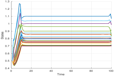
Figure 1: A typical state trajectory for our optimal control problem. Each curve depicts the state trajectory corresponding to a node of the underlying graph. The experiment was done on the Zachary’s Karate Club friendship network, with $n=34$ nodes, $T=100$ time step, and $T_{0}=10$. The initial opinion level is $0.5$ on all nodes and the threshold level is $\tau=0.7$. There are $m=5$ controlled nodes. Observe that the equilibrium values are reached shortly after $t=T_{0}$. This is evident from the fact that $\|x(12)-x^{e}\|_{2}/\|x^{e}\|_{2}=0.009$ and $\|x(15)-x^{e}\|_{2}/\|x^{e}\|_{2}=0.00076$.

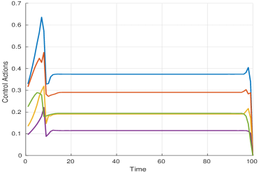
Figure 2: A typical control action trajectory for our optimal control problem. Each curve corresponds to the control actions at one of $m=5$ controlled nodes. The experimental setup is same as for Fig. 1. It can be observed that the equilibrium values are reached shortly after $t=T_{0}$.This is evident from the fact that $\|u(12)-u^{e}\|_{2}/\|u^{e}\|_{2}=0.020$ and $\|u(15)-u^{e}\|_{2}/\|u^{e}\|_{2}=0.00089$.

Figure 3: A typical state trajectory for the Group Ferment optimal control problem. Each curve depicts the state trajectory corresponding to a node of the underlying graph. The experiment was done on the Zachary’s Karate Club friendship network, with $n=34$ nodes, $T=100$ time step, and $T_{0}=10$. The initial opinion level is $0.5$ on all nodes and the threshold level is $\tau=0.7$. There are $m=5$ controlled nodes. The values of parameters $k$ and $a$ are $0.5$ and $1$ respectively.

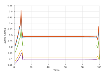
Figure 4: A typical control action trajectory for the Group Ferment optimal control problem. Each curve corresponds to the control actions at one of $m=5$ controlled nodes. The experimental setup is same as for Fig. 3.

5 Selecting an Optimal Set of Controlled Nodes

In the previous sections, we have studied the problem of finding the minimum cost control when the $m$ controlled nodes are given. We now take the design view and allow the influencing entity to choose the $m$ controlled nodes. In the discussion in this section, we restrict our attention to the case of $R=I_{m}.$ Extensions to the case of a diagonal, positive $R$ is straightforward.

The problem of choosing $m$ controlled nodes can also be seen as designing the matrix $B$ such that $m$ of its entries are $1$ and others are $0.$ For the optimal control problem (TF), this reduces to solving the following optimization problem.

$$\begin{split}&\underset{B}{\text{minimize}}~{}~{}J^{*}_{TF}(\bar{x})=\sum_{t=0}^{T-1}\|u^{*}(t)\|_{2}^{2}\\ &\text{subject to}~{}~{}\|B\|_{0}=m,\end{split}$$ (22)

where, given a particular choice of $B$, $(u^{*}(t))_{t=0}^{T-1}$ denotes an optimal control action trajectory for (TF). The optimization for (GF) is analogous with $J^{*}_{TF}(\bar{x})$ being replaced by $J^{*}_{GF}(\bar{x}).$

It must be noted that for some graph topologies, there may exist sets of controlled nodes for which an equilibrium $(x^{e},u^{e})$ does not exist. That is, there are valid matrices $B^{\dagger}$ such that there is no solution to $x^{e}=Ax^{e}+B^{\dagger}u^{e}+(I_{n}-A)q$ for $x^{e}\geq\tau$. Towards this, we invoke Lemma 4.2 which states that an equilibrium is guaranteed to exist under Assumption 3.

The state-action trajectories, before the equilibrium is reached, are difficult to analyze and this makes solving the above optimization problem hard. Recall that the turnpike property of the optimal solutions of (TF) and (GF) implies that the state-action trajectory $(x^{*}(t),u^{*}(t))_{t=0}^{T}$ remains close to an equilibrium point $(x^{e},u^{e})$, for all but a small fraction of the time steps in $(T_{0},T).$ The equilibrium point for (TF) can be found explicitly via (14). Now observe that the equilibrium $(x^{e},u^{e})$ is independent of the initial state $\bar{x}$ and the final time $T$. Hence, rather than solve (22) exactly, we can consider approximately solving the optimization problem in (22), where we optimize the choice of controlled nodes to minimize the cost incurred while the state is close to $x^{e}.$ Informally, this ensures that the cost is minimized to keep the system running in the equilibrium state. We expect this to be a good approximation, especially as the time horizon $T$ becomes large. Thus the following optimization problem is a good approximation for the exact solution of the problem of optimally selecting controlled nodes for (TF).

$$\begin{split}&\underset{B}{\text{minimize}}~{}~{}\|u^{e}\|_{2}^{2}\\ &\text{subject to}\begin{cases}x^{e}=Ax^{e}+Bu^{e}+(I_{n}-A)q\\ x^{e}\geq\tau\\ \|B\|_{0}=m.\end{cases}\end{split}$$ (23)

For problem (GF), the second constraint is replaced by $\phi(x^{e})\geq kn.$

The sparsity constraint on $B$ in (23) makes the problem non-convex and thus, hard to solve. The following two heuristics are based on the above optimization problem.

5.1 Convex Relaxation

Here we remove the constraint on $B$ in (23) and add a term in the objective function corresponding to the $l_{1}$ norm of the control, corresponding to the well-known LASSO regularization technique [31]. We define an auxiliary variable $\tilde{u}^{e}\in\mathbb{R}^{n}$ to be used in place of $Bu^{e}$ such that the resulting problem formulation is:

$$\begin{split}&\underset{\tilde{u}^{e}}{\text{minimize}}~{}~{}\|\tilde{u}^{e}\|_{2}^{2}+\mu\|\tilde{u}^{e}\|_{1}\\ &\text{subject to}\begin{cases}x^{e}=Ax^{e}+\tilde{u}^{e}+(I_{n}-A)q\\ x^{e}\geq\tau.\end{cases}\end{split}$$ (24)

Let the solution of this convex problem be $\tilde{u}^{*}$. The controlled nodes are chosen as the nodes corresponding to which $\tilde{u}^{*}$ has non-zero entries. The regularization coefficient $\mu$ can be adapted to change the sparsity level desired from the solution. However, it might not always be possible to match the sparsity of the solution to $m$, the number of controlled nodes. In such a scenario, one can select the top $m$ elements of $\tilde{u}^{*}$ to select the controlled nodes.

It must be noted here that such a convex relaxation heuristic can be used only for problem (TF) and not for problem (GF). This is because the set specifying the state constraints is convex for problem (TF) and is generally non-convex for problem (GF). In the following subsection we give an heuristic which is applicable for both the problems, (TF) and (GF).

5.2 A Greedy Heuristic

A greedy heuristic can be used for the non-convex problem (23) and the corresponding problem for (GF). In this greedy heuristic we choose one node per step of the algorithm. At each step we choose the node that causes the largest reduction in the total cost of maintaining the state at equilibrium to include into the set of controlled nodes. Algorithm 1 describes this heuristic formally for problem (TF). The algorithm for problem (GF) will be similar except for a minor change in lines 8–10 that are shown in Algorithm 2. To ensure that the intermediate steps of the algorithms have feasible solutions, we start building the set of controlled nodes with a set of nodes having direct paths to all other nodes. The existence of such a set of nodes is ensured by Assumption 3. We denote this small set of nodes by $C_{\text{init}}.$

Input: $(A,q,\tau,m,n)$

Output: Set of controlled nodes

1 Let C be the set of controlled nodes

$C=C_{\text{init}}$

  $\backslash\backslash$ initialization

2 for $i\leftarrow 1$ to $m$ do

3       $n_{i}=\underset{j\in\mathcal{N}\backslash C}{\arg\min}~{}equilibrium\_cost(C\cup\{j\})$

       $C\leftarrow C\cup n_{i}$

        $\backslash\backslash$ greedy update

4      

5 end for

1 Procedure $equilibrium\_cost$(S)

2       $B=0_{m\times n}$

       $i=1$

        $\backslash\backslash$ counter variable

3       for $j\in S$ do

             $B(j,i)=1$

              $\backslash\backslash$ designing $B$ using $S$

4             $i=i+1$

5            

6       end for

7      

8      $\text{minimize}~{}~{}\|u^{e}\|_{2}^{2}$

9       subject to $\begin{cases}x^{e}=Ax^{e}+Bu^{e}+(I_{n}-A)q\\ x^{e}\geq\tau\end{cases}$

10       return $\|u^{e}\|_{2}^{2}$

11

12

Algorithm 1 Greedy heuristic for controlled node selection for problem (TF)

1 $\underset{u}{\text{minimize}}~{}~{}J_{GF}(\bar{x},u)=\sum_{t=0}^{T-1}\|u(t)\|^{2}_{2}$

2 subject to $\begin{cases}\text{state~{}dynamics~{}\eqref{eq:dynamics}},\\ \text{state~{}constraints~{}\eqref{eq:group-ferment}}\\ x(0)=\bar{x}\in\mathbb{R}^{n}\text{~{}(given).}\end{cases}$

3 return $J_{GF}(\bar{x},u)$

4

Algorithm 2 Lines 8–10 in Algorithm 1 should be replaced by this segment to obtain the $m$ controlled nodes for problem (GF) using the greedy heuristic.

6 Max Min Optimal Control

To solve the problem (MF), we need to define the following two system variables in addition to $x(t)\in\mathbb{R}^{n},$ the opinion at each of the nodes at time $t.$

• $r(t)\in\mathbb{R}$ is the record of $\psi(x(\cdot))$ up to time $t,$ i.e., it is the minimum value of $\psi(x(\cdot))$ till time $t-1.$ Formally,

  $$r(t)=\begin{cases}\psi(x(0))&t=0\\ \min_{0\leq\tau\leq t-1}~{}~{}\psi(x(\tau))&t=1,\ldots,T,\end{cases}$$ (25)

• $y(t)\in\mathbb{R},$ is the running sum of the control cost till time $t-1,$ i.e.,

  $$y(t)=\begin{cases}0&t=0\\ \sum_{\tau=0}^{t-1}c(u(\tau))&t=1,\ldots,T,\end{cases}$$ (26)

  subject to the budget constraint, imposed by the boundary condition

  $$y(T)\leq C.$$ (27)

We can see that problem (MF) is equivalent to maximizing $r(T)$ subject to the budget constraint $y(T)\leq C$ and the given initial conditions. Thus we can use $x(t),$ $r(t),$ and $y(t)$ as the state variables in an optimal control problem. The dynamics of these state variables will be as follows.

$$\begin{split}x(t+1)&=f(x(t),u(t))~{}~{}~{}~{}~{}~{}~{}~{}~{}~{}\text{for~{}}t=0,\ldots,T-1,\\ r(t+1)&=\min\{r(t),\psi(x(t))\}~{}~{}\text{for~{}}t=0,\ldots,T-1,\\ y(t+1)&=y(t)+c(u(t))~{}~{}~{}~{}~{}~{}~{}~{}\text{for~{}}t=0,\ldots,T-1.\end{split}$$ (28)

Observe that the dynamics of the state variable $r(t)$ are generally not smooth. This implies that the classical PMP cannot be used to solve the problem (MF).

Optimal control with minimax cost has been studied before; see [7], the authoritative monograph and the references therein for a general introduction to the problem and the issues. Here, we use some recent results on non-smooth PMP obtained in [24], and develop a numerical technique to solve the optimal control problem (MF) exactly. The non-smooth PMP solution based on [24], is discussed in the following subsection.

6.1 Non-smooth PMP formulation

Consider the problem (MF). Let $(x^{*}(t),r^{*}(t),y^{*}(t))_{t=0}^{T}$ and $(u^{*}(t))_{t=0}^{T-1}$ be an optimal state-action trajectory that solves (MF). Define the Hamiltonian

$$\mathbb{R}^{n}\times\mathbb{R}\times\mathbb{R}\times\mathbb{R}^{n}\times\mathbb{R}\times\mathbb{R}\times\mathbb{R}^{m}\ni(\zeta_{x},\zeta_{r},\zeta_{y},\xi_{x},\xi_{r},\xi_{y},\mu)$$

$$\mapsto H(\zeta_{x},\zeta_{r},\zeta_{y},\xi_{x},\xi_{r},\xi_{y},\mu):=\zeta_{x}^{\intercal}\left(A\xi_{x}+B\mu+(I_{n}-A)q\right)$$

$$+\zeta_{r}\min\{\xi_{r},\psi(\xi_{x})\}+\zeta_{y}(\xi_{y}+c(\mu)).$$

Let the adjoint variables be given by $(\lambda_{x}(t),\lambda_{r}(t),\lambda_{y}(t))_{t=0}^{T}$. For ease of notation, we use $\lambda(t)$ in place of $(\lambda_{x}(t),\lambda_{r}(t),\lambda_{y}(t))$ and $\lambda_{xr}(t)$ to denote the tuple $(\lambda_{x}(t),\lambda_{r}(t))$. Similarly we use $xr^{*}(t)$ to denote the tuple $(x^{*}(t),r^{*}(t))$. The non-smooth PMP asserts that there exists a sequence $(\lambda(t))_{t=0}^{T}$ that satisfy the following.

• The adjoint variable $\lambda^{*}(t)$ does not vanish at any time.

• The state dynamics follow

  $$\begin{split}x^{*}(t+1)=\frac{\partial}{\partial\zeta_{x}}H(\lambda^{*}(t),x^{*}(t),r^{*}(t),y^{*}(t),u^{*}(t))\\ r^{*}(t+1)=\frac{\partial}{\partial\zeta_{r}}H(\lambda^{*}(t),x^{*}(t),r^{*}(t),y^{*}(t),u^{*}(t))\\ y^{*}(t+1)=\frac{\partial}{\partial\zeta_{y}}H(\lambda^{*}(t),x^{*}(t),r^{*}(t),y^{*}(t),u^{*}(t))\\ \text{for~{}}t=0,\ldots,T-1.\end{split}$$ (29)

• The adjoint dynamics [24] follow

  $$\begin{split}&\lambda_{y}(t-1)=\frac{\partial}{\partial\xi_{y}}H(\lambda^{*}(t),x^{*}(t),r^{*}(t),y^{*}(t),u^{*}(t))\\ &\left<\lambda_{xr}(t-1),v\right>\geq\mathcal{D}_{v}H(\lambda^{*}(t),\cdot,\cdot,y^{*}(t),u^{*}(t))(xr^{*}(t))\\ &\text{for all~{}}v\in\mathbb{R}^{n+1},\text{~{}for~{}}t=1,\ldots,T-1.\end{split}$$ (30)

• Since the objective is to maximize $r(T)$, the following terminal conditions are satisfied:

  $$\lambda_{r}(T)=1,$$ (31)

  $$\lambda_{x}(T)=0.$$ (32)

• The following complementary slackness condition is satisfied.

  $$\lambda_{y}(T)(y^{*}(T)-C)=0.$$ (33)

• The following Hamiltonian maximization condition is satisfied.

  $$\frac{\partial}{\partial\mu} H(\lambda^{*}(t),x^{*}(t),r^{*}(t),y^{*}(t),u^{*}(t))=0,$$ (34)

  $${\color[rgb]{0,0,0}{\text{i.e.,~{}}u^{*}(t)=\frac{1}{2\lambda^{*}_{y}(T)}R^{-1}B^{\intercal}\lambda_{x}^{*}(t).}}$$ (35)

The case of $\lambda^{*}_{y}(T)=0$ corresponds to the existence of abnormal control. It must also be noted that the non-smooth PMP, similar to PMP, is based on first order conditions and does not guarantee the uniqueness of the solution obtained. It must be noted here that the non-smooth PMP uses directional derivatives to specify the dynamics of the adjoint variables; see definition below.

Definition 6.1.

([10], Section 1.4 on page 20) Let $g:\mathbb{R}^{d}\times\mathbb{R}^{m}\to\mathbb{R}^{n}$ be a continuous map. For $y\in\mathbb{R}^{m}$ and a vector $v\in\mathbb{R}^{d}$, we denote by $\mathcal{D}_{v}g(\cdot,y)(x)$ the directional derivative of $g(\cdot,y)$ along $v$ at $x$, whenever the following limit exists:

$$\mathcal{D}_{v}g(\cdot,y)(x):=\lim_{\theta\downarrow 0}\frac{g(x+\theta v,y)-g(x,y)}{\theta}$$ (36)

Note that the directional derivative above is defined as a right-hand (one-sided) limit. If $g$ is continuously differentiable, then $\mathcal{D}_{v}g(\cdot,y)(x)=\frac{\partial}{\partial x}g(x,y).v$.

In the following we develop a modified forward-backward sweep algorithm to find a numerical solution of problem (MF) satisfying the conditions of the non-smooth PMP. In the next subsection, we outline the algorithm.

6.2 Numerical Algorithm

Before we discuss the algorithm, we analyze the directional derivative of the Hamiltonian for problem (MF). We denote the ordered pair of vector $v_{x}\in\mathbb{R}^{n}$ and scalar $v_{r}\in\mathbb{R}$ by $v,$ such that $\mathbb{R}^{n}\times\mathbb{R}\ni v=(v_{x},v_{r})$.

$$\mathcal{D}_{v}H(\lambda,\cdot,\cdot,y,u)(xr)$$

$$=\lim_{\theta\downarrow 0}\frac{H(x+\theta v_{x},r+\theta v_{r},y,u)-H(x,r,y,u)}{\theta}$$ (37)

Here we consider three cases for the the relation between $r(t)$ and $\psi(x(t))$ to determine the directional derivatives which will then give the adjoint dynamics.

• Case 1: for some time instant $t=t_{1},$ we have $r(t_{1})<\psi(x(t_{1}))$. In this case, the record state $r(t_{1}+1)$ is updated such that $r(t_{1}+1)=r(t_{1})$. The non-smooth PMP formulation is same as the usual PMP because the Hamiltonian is differentiable in all the state variables. The adjoint dynamics at this time instant are given by

  $$\lambda_{y}(t_{1}-1) =\lambda_{y}(t_{1}),$$

  $$\lambda_{r}(t_{1}-1) =\lambda_{r}(t_{1}),$$

  $$\lambda_{x}(t_{1}-1) =A^{\intercal}\lambda_{x}(t_{1}).$$

• Case 2: For some time instant $t=t_{2},$ we have $r(t_{2})>\psi(x(t_{2}))$. In this case, the record state $r(t_{2}+1)$ is updated such that $r(t_{2}+1)=\psi(x(t_{2}))$. The non-smooth PMP formulation is same as the usual PMP because the Hamiltonian is differentiable in all the state variables. The adjoint dynamics at this time instant are given by

  $$\lambda_{y}(t_{2}-1) =\lambda_{y}(t_{2}),$$

  $$\lambda_{r}(t_{2}-1) =0,$$

  $$\lambda_{x}(t_{2}-1) =A^{\intercal}\lambda_{x}(t_{2})+\lambda_{r}(t_{2})\frac{d}{dx}\psi(x(t_{2})).$$

• Case 3: For some time instant $t=t_{3},$ we have $r(t_{3})=\psi(x(t_{3}))$. In this case the non-smooth PMP formulation is not the same as the usual PMP because the Hamiltonian is not differentiable in all the state variables. Using the directional derivatives, the adjoint dynamics at the time instant $t_{3}$ are given by

  $$\lambda_{y}(t_{3}-1)=\lambda_{y}(t_{3}),$$

  $$\left<\lambda_{r}(t_{3}-1),v_{r}\right>+\left<\lambda_{x}(t_{3}-1),v_{x}\right>$$

  $$\geq\mathcal{D}_{v}H(\lambda(t_{3}),\cdot,\cdot,y(t_{3}),u(t_{3}))(xr(t_{3}))$$

  $$\text{for all~{}}v_{x}\in\mathbb{R}^{n}\text{~{}and all~{}}v_{r}\in\mathbb{R}.$$

  The directional derivative, in direction $v$, at the time $t_{3}$ instant can be given by:

  $$\lambda_{x}^{\intercal}(t_{3})Av_{x}+\lambda_{r}(t_{3})\min\left\{\left<\frac{d}{dx}\psi(x(t_{3})),v_{x}\right>,v_{r}\right\}.$$ (38)

  A proof of (38) is in Appendix A.2.

  The adjoint dynamics are:

  $$\lambda_{y}(t_{3}-1)=\lambda_{y}(t_{3}),$$

  $$\left<\lambda_{r}(t_{3}-1),v_{r}\right>+\left<\lambda_{x}(t_{3}-1),v_{x}\right>$$

  $$\geq\lambda_{x}^{\intercal}(t_{3})Av_{x}+\lambda_{r}(t_{3})\min\left\{\left<\frac{d}{dx}\psi(x(t_{3})),v_{x}\right>,v_{r}\right\}$$ (39)

  $$\text{for all~{}}v_{x}\in\mathbb{R}^{n}\text{~{}and all~{}}v_{r}\in\mathbb{R}.$$

  Here we consider the following two possibilities:

  $$\left<\frac{d}{dx}\psi(x(t_{3})),v_{x}\right>\geq v_{r},$$

  $$\left<\frac{d}{dx}\psi(x(t_{3})),v_{x}\right><v_{r}.$$

  We need $\lambda_{x}(t_{3}-1)$ and $\lambda_{r}(t_{3}-1)$ to be such that (39) is satisfied for both the above stated possibilities. We use the following values of $\lambda_{x}(t_{3}-1)$ and $\lambda_{r}(t_{3}-1)$:

  $$\begin{split}\lambda_{x}(t_{3}-1)&=A^{\intercal}\lambda_{x}(t_{3})+\phi\lambda_{r}(t_{3})\frac{d}{dx}\psi(x(t_{3})),\\ \lambda_{r}(t_{3}-1)&=(1-\phi)\lambda_{r}(t_{3}),\\ \text{for some~{}}\phi&\in[0,1].\end{split}$$ (40)

  We now verify that this indeed satisfies (39).

  When $\left<\frac{d}{dx}\psi(x(t_{3})),v_{x}\right>>v_{r},$ (39) reduces to:

  $$\left<\lambda_{r}(t_{3}-1),v_{r}\right>+\left<\lambda_{x}(t_{3}-1),v_{x}\right>$$

  $$\geq\lambda_{x}^{\intercal}(t_{3})Av_{x}+\lambda_{r}(t_{3})v_{r}.$$ (41)

  Using the adjoint dynamics given by (40), we see that

  $$\left<\lambda_{r}(t_{3}-1),v_{r}\right>+\left<\lambda_{x}(t_{3}-1),v_{x}\right>=\left<(1-\phi)\lambda_{r}(t_{3}),v_{r}\right>$$

  $$+\left<A^{\intercal}\lambda_{x}(t_{3})+\phi\lambda_{r}(t_{3})\frac{d}{dx}\psi(x(t_{3})),v_{x}\right>$$

  $$=\lambda_{x}^{\intercal}(t_{3})Av_{x}+(1-\phi)\lambda_{r}(t_{3})v_{r}$$

  $$+\phi\lambda_{r}(t_{3})\left<\frac{d}{dx}\psi(x(t_{3})),v_{x}\right>$$

  $$\geq\lambda_{x}^{\intercal}(t_{3})Av_{x}+\lambda_{r}(t_{3})v_{r}$$

  $$\text{for~{}}\phi\lambda_{r}(t_{3})\geq 0,$$ (42)

  thus satisfying (41) if $\phi\lambda_{r}(t_{3})\geq 0$.

  Now we consider the second case, i.e., when $\left<\frac{d}{dx}\psi(x(t_{3})),v_{x}\right><v_{r}$. In this case, condition (39) reduces to:

  $$\left<\lambda_{r}(t_{3}-1),v_{r}\right>+\left<\lambda_{x}(t_{3}-1),v_{x}\right>$$

  $$\geq\lambda_{x}^{\intercal}(t_{3})Av_{x}+\lambda_{r}(t_{3})\left<\frac{d}{dx}\psi(x(t_{3})),v_{x}\right>.$$ (43)

  From the adjoint dynamics in (40), we see that

  $$\left<\lambda_{r}(t_{3}-1),v_{r}\right>+\left<\lambda_{x}(t_{3}-1),v_{x}\right>=\left<(1-\phi)\lambda_{r}(t_{3}),v_{r}\right>$$

  $$+\left<A^{\intercal}\lambda_{x}(t_{3})+\phi\lambda_{r}(t_{3})\frac{d}{dx}\psi(x(t_{3})),v_{x}\right>$$

  $$=\lambda_{x}^{\intercal}(t_{3})Av_{x}+(1-\phi)\lambda_{r}(t_{3})v_{r}$$

  $$+\phi\lambda_{r}(t_{3})\left<\frac{d}{dx}\psi(x(t_{3})),v_{x}\right>$$

  $$\geq\lambda_{x}^{\intercal}(t_{3})Av_{x}+\lambda_{r}(t_{3})\left<\frac{d}{dx}\psi(x(t_{3})),v_{x}\right>$$

  $$\text{for~{}}(1-\phi)\lambda_{r}(t_{3})\geq 0,$$ (44)

  thus satisfying (43) if $(1-\phi)\lambda_{r}(t_{3})\geq 0$. To satisfy both (41) and (43), we need to satisfy both $\phi\lambda_{r}(t_{3})\geq 0$ and $(1-\phi)\lambda_{r}(t_{3})\geq 0$. This implies $\lambda_{r}(t_{3})\geq\phi\lambda_{r}(t_{3})\geq 0$ and therefore $\phi\in[0,1]$. This verifies that our design in 40 satisfies 39. Note that this is valid only for $\lambda_{r}(t_{3})\geq 0,$ which follows the terminal conditions (31) and the dynamics of $\lambda_{r}(\cdot)$ ensuring that it doesn’t change its sign. The exact value of $\phi$ is determined by the algorithm to ensure the required relation between $r(t_{3})$ and $\psi(x(t))$.

The detailed algorithm is described in Algorithm 3. The value of the adjoint variable $\lambda_{y}(T)$ is determined by the shooting method, implemented in the outer loop of Algorithm 3, such that the complementary slackness conditions (33) are satisfied.

Input: $A,B,Budget,\bar{x},\varepsilon_{1},\varepsilon_{2},w,\mu$

Output: Optimal state-action trajectory $(x^{*},u^{*})$

1 Set: $\lambda_{x}(T)=0,$ $\lambda_{r}(T)=1$.

2 Initialize: $\lambda_{y}^{(0)}(T)=1.$

3 repeat

4       Initialize: $u^{(0)}=0$.

5       repeat

6             Forward Sweep: Find $x^{(j)}$ using $u^{(j)}$ via (28).

7             Backward Sweep:

8            $\tilde{u}=Backward\left(\lambda_{x}(T),\lambda_{r}(T),\lambda_{y}^{(p)}(T),x^{(j)}\right)$

9             $u^{(j+1)}=wu^{(j)}+(1-w)\tilde{u}$

10      until $j^{*}\text{such that~{}}\left\|u^{(j^{*})}-u^{(j^{*}-1)}\right\|_{F}<\varepsilon_{1}$

11      $Expenditure=\sum_{t=0}^{T-1}c\left(u^{(j^{*})}(t)\right)$

12       $\lambda_{y}^{(p+1)}(T)=\lambda_{y}^{(p)}(T)-\mu(Expenditure-Budget)$

13      

14until $p^{*}\text{such that~{}}\left|\lambda_{y}^{(p^{*})}(T)-\lambda_{y}^{(p^{*}-1)}(T)\right|<\varepsilon_{2}$

15$u^{*}=u^{(j^{*})},$ $x^{*}$ from $u^{*}$ via (28).

16 Procedure $Backward$($\lambda_{x}(T),\lambda_{r}(T),\lambda_{y}^{(p)}(T),x^{(j)}$)

17       for $\tau\leftarrow T-1$ to $0$ do

18             Find $\phi$ such that $\psi(x(\tau))=\psi(x(\tau+1))$,

19             with adjoint dynamics (40) and control (35).

20             if $\phi>1$ then

21                  $\lambda_{x}(\tau)=A^{\intercal}\lambda_{x}(\tau+1)+\lambda_{r}(\tau+1)\left<\frac{d}{dx}\psi(x(\tau+1))\right>$

22                   $\lambda_{r}(\tau)=0$

23                   $\lambda_{y}(\tau)=\lambda_{y}(\tau+1)$

24             else if $\phi<0$ then

25                  $\lambda_{x}(\tau)=A^{\intercal}\lambda_{x}(\tau+1)$

26                   $\lambda_{r}(\tau)=\lambda_{r}(\tau+1)$

27                   $\lambda_{y}(\tau)=\lambda_{y}(\tau+1)$

28             else

29                  $\lambda_{x}(\tau)=A^{\intercal}\lambda_{x}(\tau+1)+\phi\lambda_{r}(\tau+1)\left<\frac{d}{dx}\psi(x(\tau+1))\right>$

30                   $\lambda_{r}(\tau)=(1-\phi)\lambda_{r}(\tau+1)$

31                   $\lambda_{y}(\tau)=\lambda_{y}(\tau+1)$

32             end if

33             $\tilde{u}(\tau)=\frac{1}{2\lambda_{y}^{(p)}(T)}R^{-1}B^{\intercal}\lambda_{x}(\tau)$

34       end for

35      return $\tilde{u}$

36

Algorithm 3 Numerical algorithm to solve the maxmin ferment problem

7 Numerical Results

In this section we report the results from a subset of the extensive numerical experiments that we performed. For the (TF) problem, we first study the performance of our algorithm to choose the controlled nodes and compare it against some natural heuristics. We show that our algorithm is better. We then study the effect on the cost of maintaining ferment as a function of different parameters—structure of the network, the threshold level, the number of controlled nodes, and the stubbornness of the nodes. For all these experiments, the results for the (GF) problem are qualitatively similar to that of (TF) and we can draw similar conclusions. Hence we do not report those results. However, we do study the effect of parameters $a$ and $k$ on the cost of maintaining ferment and also analyze the opinion levels at the nodes in the network. Finally, for the (MF) problem, we study the behavior of the minimum value that is attained as a function of the budget.

The setup for the experiments is as follows. For all the experiments, the influence matrix $A$ is such that the sum of each row of $A$ is $0.9$, making it sub-stochastic. Further, each agent places equal weight on its opinion and that of each of its neighbors. This means that for any node $i$ and each of its neighbors $j$, $a_{ii}=a_{ji}=0.9/(N_{i}+1)$ where $N_{i}$ is the number of in-neighbors of $i.$ The initial opinions are taken as $\bar{x}=0.5$ and the quiescent level is set to $q=0$ such that the opinion recedes to zero in the absence of external control. The threshold level $\tau_{i}$ is set to $0.7$ for all $i.$ The system is studied for $T=100$ time steps and the threshold level is enforced from $T_{0}=10$ onwards. For all the experiments, we take the matrix $R$ in the cost function (4) to be the identity matrix $I_{m}.$ We use the open source software CasADi[4] for numerical simulations. The state-action trajectories obtained from CasADi are verified to satisfy the necessary conditions obtained using PMP in Section 3. Our experiments are performed on three kinds of random networks, each with $n=50$ nodes—the Erdős-Rènyi (ER) graphs [12], Barabàsi-Albert (BA) graphs [6], and $k$-regular graphs ($k$R). Finally, the results are averaged over $100$ realizations of the random network topology. The standard deviations in the results are also indicated on the plots. The height of the bar on one side of the point is equal to the standard deviation in $100$ random realizations.

It must noted that the initial conditions of the states are not crucial to the results of the simulation tests. As seen earlier in the paper, the equilibrium state-control trajectories are independent of the initial conditions. For $T$ large in comparison to $T_{0}$, the initial conditions have negligible effect on the total costs of maintaining ferment.

7.1 Total Ferment  (TF)

We begin by studying the impact of several model parameters on the cost of the (TF) problem.

7.1.1 Choosing controlled nodes

Social network literature provides several notions of centrality and we investigate the performance when such ‘central nodes’ are used as controlled nodes. We consider two such criteria

• Nodes with high out-degrees are clearly more influential than those with lower out-degrees. Degree centers of a graph is the set of nodes with the highest out-degree.

• Nodes that are close to a large number of nodes can propagate a control signal quicker than others. Distance center of a graph is the set of nodes that have the minimum eccentricity (largest hop-distance from the node to any other node).

We compare the cost of maintaining ferment when the set of $m$ controlled nodes are chosen to be the degree centers, the distance centers, and chosen using the convex relaxation described in Section 5.1 and using the greedy algorithm described in Section 5.2. Finding the distance center is in general NP-hard, and we instead use a greedy approximation algorithm [20]. The results for the three kinds of random networks, each with $n=50$ nodes and an average degree of $6$, are tabulated in Tables 1–Table 3.

Method	$m=2$	$m=4$	$m=6$	$m=8$	$m=10$
Greedy	174.94	95.90	71.01	58.13	48.81
Convex	181.38	105.45	83.67	72.31	65.08
Degree centers	180.36	102.18	76.79	63.33	54.69
Distance centers	1392.05	707.10	478.16	358.00	287.09

Table 1: Cost of maintaining ferment in BA networks.

Method	$m=2$	$m=4$	$m=6$	$m=8$	$m=10$
Greedy	607.18	276.57	181.24	136.59	110.15
Convex	669.55	311.03	195.97	142.31	120.44
Degree centers	680.96	325.52	216.67	166.65	137.98
Distance centers	3730.61	1606.88	921.27	626.96	451.36

Table 2: Cost of maintaining ferment in a ER networks.

Method	$m=2$	$m=4$	$m=6$	$m=8$	$m=10$
Greedy	1535.32	645.99	397.86	284.13	220.00
Convex	2003.55	825.47	481.33	326.47	251.48
Degree centers	1961.74	817.46	502.07	346.07	261.73
Distance centers	1811.33	761.41	471.87	336.70	256.54

Table 3: Cost of maintaining ferment in $k$R networks.

From the Tables 1–Table 3, we see that the greedy algorithm performs the best in all cases. It is also observed that the distance centres performs very poorly for the BA and ER graphs, while its performance is comparable to the other heuristics for the $k$R graph. One reason why distance centres perform so badly for the BA and ER graphs is that it sometimes fails to pick the nodes with the larger out-degrees, which can have large influence in the network. In the $k$R graphs, this heuristic is good because all nodes have equal out-degrees. On the other hand, the degree centers heuristic picks the nodes with the highest out-degrees and thus performs fairly well. However, it is not the best scheme as it does not account for the distance to other nodes while selecting the controlled nodes. The convex relaxation heuristic also performs comparably to the degree centers but not as good as the greedy heuristic. Given these results, in all of the following experiments, we will use the greedy algorithm for selecting the controlled nodes.

7.1.2 Effect of Network Structure

Here we study the variation of the cost of maintaining ferment with the average degree and the degree distribution of the network. The variation in the degree distributions is provided by the different networks. For each given average degree, we consider the BA graphs with the power law degree distribution, the Erdős-Rènyi (ER) graphs [12] with binomial degree distribution and the random regular graphs with constant degree. Each network consists of $n=50$ nodes with $m=5$ controlled nodes, chosen according to the greedy heuristic presented in Section 5.2. We plot the results in Fig. 5.

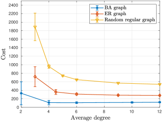
Figure 5: Cost of maintaining ferment as a function of average degree.

From Fig. 5, we see that it is cheaper to maintain ferment in a network with a higher average degree but the marginal gain decreases rather rapidly with increasing degree. This is to be expected since once the graph is fairly well-connected, all nodes are easily accessible and increasing the degree further has minimal benefit. For a given average degree, we also see that the cost is the least for the BA network and and highest for $k$R graphs, indicating that the presence of nodes with high degrees makes it easier to maintain the ferment.

7.1.3 Effect of Threshold Value

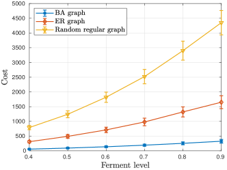
Figure 6: Cost of maintaining ferment as a function of desired ferment level.

In Fig. 6, we plot the cost of maintaining ferment as a function of the threshold $\tau.$ The cost is approximately quadratic with respect to $\tau.$ This is to be expected since the cost function is a quadratic. In keeping with the finding from the previous experiment, the cost is highest in the $k$R graphs and lowest for BA graphs. The effect of the degree distribution is noteworthy with significant cost reductions being obtained when there are a few nodes with large degrees as in the BA graph.

7.1.4 Number of Controlled Nodes

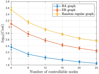
Figure 7: Cost of maintaining ferment as a function of the number of controlled nodes.

Fig. 7 shows the cost of maintaining ferment as a function of $m,$ the number of controlled nodes. Note that the cost is plotted on a logarithmic scale indicating that the reduction in cost is quite steep. This sharp reduction in cost is due to two reasons: firstly, as the cost function for control inputs is convex, having to apply smaller control inputs at a larger number of controlled nodes decreases the total cost. The second reason is that having a larger number of controlled nodes decreases the average distance of nodes from a controlled node, thus helping reduce the control inputs required to influence the most remote nodes.

7.1.5 Effect of Stubbornness

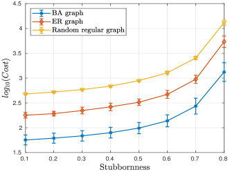
Figure 8: Cost of maintaining ferment as a function of the stubbornness of agents when all the agents are stubborn.

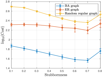
Figure 9: Cost of maintaining total ferment: $80\%$ agents have $a_{ii}=0,$ plot of cost vs $a_{ii}$ of stubborn nodes.

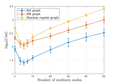
Figure 10: Cost of maintaining ferment as a function of the number of stubborn agents; $a_{ii}=0.7$ for each stubborn agent.

Recall that in (1), $a_{ii}$ denotes the stubbornness of node $i.$ We now study its effect on the cost of maintaining ferment. In the first set of experiments we assume that $a_{ii}$ is the same for all $i.$ The $a_{ji}$ are calculated as before, i.e., $a_{ji}=(0.9-a_{ii})/N_{i}$ where $N_{i}$ is the number of in-neighbors of $i.$ Fig. 8 plots the cost as a function of $a_{ii}.$ We see that the cost increases very rapidly with an increase in the stubbornness of the agents in the network. This indicates that a thorough understanding of the population stubbornness is vital before starting a campaign for maintaining ferment on a topic for a certain period of time.

Next, we repeat this experiment except that now only a fraction ($20\%$) of the nodes are stubborn, chosen at random from the network. The cost of maintaining ferment as a function of $a_{ii}$ is plotted in Fig. 9. Here the results are very different from the case of all agents being stubborn. The cost first decreases with the level of stubbornness $a_{ii}$ and then increases. The decrease can be explained as the stubborn nodes are good candidates for controlled nodes. The increase, seen for a very high level of stubbornness is because of those stubborn nodes which were not chosen as controlled nodes. Recall that in this experiment, there are $m=5$ controlled nodes and $10$ stubborn nodes.

We also perform another variation of this experiment with a varying fraction of the agents being stubborn. The stubbornness of the stubborn agents is set to $a_{ii}=0.7$, and the number of stubborn agents is varied from $0$ to $50$. The results of this experiment are in Fig. 10. It can be seen that the cost of maintaining ferment is smallest when the number of stubborn nodes is $5$ for all three types of networks. This is equal to the number of controlled nodes, $m=5$ and stubborn nodes make good controlled nodes. This is backed by the observation that when the number of stubborn nodes is $5$, on average, $4.19$, $4.52$, and $4.97$ controlled nodes are stubborn in the ER, BA, and $k$R graphs respectively. The cost increases with increasing number of stubborn nodes, beyond $5$. This is because these additional stubborn nodes are not controlled and thus they lead to a higher cost of maintaining ferment.

7.2 Group Ferment (GF)

We will now consider the (GF) problem. For all the experiments conducted above, the results for the (GF) problem are qualitatively similar to that of (TF) and we can draw similar conclusions. Hence we do not report those results. We will instead study the effect of parameters $a$ and $k$ on the cost of maintaining group ferment.

7.2.1 Effect of $a$ and $k$

Recall that $a$ is the slope parameter of the sigmoid function and $k$ is the fraction that determines the level of group ferment to be maintained. As before, we take the number of nodes in the network to be $n=50$, the average degree is set to $6$, and the threshold parameter $\tau$ is set to $0.7$. The system is observed for $T=100$ time steps and the setup time $T_{0}=10$. The number of controlled nodes is $m=5$ and they are chosen by using the greedy heuristic. As before, the results are averaged over $100$ realizations of the network topology. In Tables 4, 5, and 6, we tabulate the average cost of maintaining group ferment as a function of the parameters $a:$ slope of sigmoid function and $k:$ the level of group ferment desired. We do this experiment for the ER, BA, and $k$R graphs.

$a$ $\downarrow$    $k$ $\rightarrow$	$0.5$	$0.6$	$0.7$	$0.8$
$1$	44.40	115.77	234.56	441.10
$3$	44.61	65.64	93.92	136.27
$5$	44.97	57.91	74.24	97.24
$7$	45.38	55.10	66.95	83.05
$10$	45.95	53.37	62.09	77.39

Table 4: Cost of maintaining group ferment in BA networks as a function of $a,$ slope of sigmoid function and $k,$ level of desired group ferment.

$a$ $\downarrow$    $k$ $\rightarrow$	$0.5$	$0.6$	$0.7$	$0.8$
$1$	253.99	681.72	1427.35	2762.23
$3$	267.60	406.50	594.21	876.89
$5$	281.17	369.05	477.83	632.44
$7$	289.95	355.42	433.38	542.56
$10$	296.80	345.79	403.86	482.92

Table 5: Cost of maintaining group ferment in $k$R networks as a function of $a,$ slope of sigmoid function, and $k,$ level of group ferment desired.

$a$ $\downarrow$    $k$ $\rightarrow$	$0.5$	$0.6$	$0.7$	$0.8$
$1$	114.06	301.50	622.50	1195.90
$3$	106.94	160.59	234.19	344.85
$5$	109.76	144.22	187.78	248.73
$7$	112.18	138.62	170.57	213.49
$10$	105.56	124.47	146.59	175.17

Table 6: Cost of maintaining group ferment in ER networks as a function of parameters $a,$ slope of sigmoid function, and $k,$ level of group ferment desired.

In Tables 4, 5, and 6, note that the cost is increasing with increase in the parameter $k$. This is to be expected because a larger value of $k$ implies a stricter ferment requirement. For most values of $k$, the cost decreases with an increase in the slope parameter $a$. A higher value of $a$ implies that the sigmoid function used in the group ferment requirement resembles the step function more closely, which in turn means that the condition can be satisfied by targeting control on to a smaller fraction of nodes and ignoring the nodes which are more difficult to influence. It can also be observed that the increments in the cost with $k$ are larger for smaller values of $a$. This is because a smaller value of $a$ implies that the sigmoid function has a smaller slope and a larger value of control is required to achieve the same increase in $\phi(x(\cdot)).$

We also tabulate the average number of nodes whose opinion values are actually above the threshold at equilibrium when the control is applied to maintain group ferment. From Tables 7, 8, and 9, it can be seen that group ferment can be obtained by taking a smaller number of nodes above the threshold for smaller values of $k$. However for a higher value of $k,$ the group ferment is ensured only when a larger number of nodes are above the threshold, and as seen in Tables 4, 5, and 6, this comes at an increased cost. It can be seen that for some small values of $k,$ $a$ needs to be large to achieve the objective of having $kn$ nodes above $\tau.$

$a$ $\downarrow$    $k$ $\rightarrow$	$0.5$	$0.6$	$0.7$	$0.8$
$1$	17.10	50.00	50.00	50.00
$3$	17.23	44.63	50.00	50.00
$5$	17.68	39.35	47.41	50.00
$7$	19.32	36.21	45.13	49.31
$10$	20.06	34.01	42.24	48.03

Table 7: Average number of nodes with opinions above threshold at equilibrium in the (GF) problem in BA networks, as a function of the parameters $a:$ slope of sigmoid function and $k:$ the level of group ferment desired.

$a$ $\downarrow$    $k$ $\rightarrow$	$0.5$	$0.6$	$0.7$	$0.8$
$1$	7.54	50.00	50.00	50.00
$3$	12.70	38.61	50.00	50.00
$5$	18.51	34.17	48.97	50.00
$7$	23.11	33.54	44.46	49.91
$10$	27.03	33.32	37.77	48.74

Table 8: The average number of nodes which are actually above the threshold at equilibrium in the (GF) problem in $k$R networks, as a function of the parameters $a:$ slope of sigmoid function and $k:$ the level of group ferment desired.

$a$ $\downarrow$    $k$ $\rightarrow$	$0.5$	$0.6$	$0.7$	$0.8$
$1$	17.66	49.81	50.00	50.00
$3$	17.58	34.91	45.58	45.83
$5$	18.83	31.78	41.91	45.75
$7$	20.49	30.31	38.33	45.35
$10$	19.26	26.73	32.50	39.77

Table 9: The average number of nodes which are actually above the threshold at equilibrium in the (GF) problem in ER networks, as a function of the parameters $a:$ slope of sigmoid function and $k:$ the level of group ferment desired.

7.3 Maxmin Ferment  (MF)

Finally, we study the (MF) problem. Specifically, we plot the maxmin ferment level attained as a function of the available budget. The underlying graph has $n=50$ nodes and the average degree is $6$. The threshold parameter $\tau$ is set to $0.7$. The system is observed for $T=100$ time steps. The initial opinion level is set to a high value, $\bar{x}_{i}=2~{}\forall i\in[1,\ldots,n]$. The slope parameter $a=0.5$. The number of controlled nodes is $m=5$ and they are chosen by the degree centres heuristic. For this problem, we choose the degree centres heuristic instead of the greedy heuristic because the greedy heuristic is based upon the condition that the Turnpike property is present in the state-control trajectories, which is not true for this problem. On the other hand, the degree centres heuristic is more general in definition and scope. The results corresponding to BA, ER and $k$R networks are in Fig. 11 where the value of $\underset{t}{\text{minimum~{}}}\psi(x(t))$ is plotted as a function of the budget. Each point on the plot represents the average ferment and average budget across $50$ observations of the random graph topologies. Since we use a iterative algorithm to converge to the intended budget value, we also collect data points corresponding to the sample path and then bin the observations into $10$ groups. The average budget and the average ferment for each bin is plotted. It can be seen that the ferment is costliest for the $k$R graph and cheapest for the BA graph. The results corresponding to larger values of $a$ could not be attained due to stability issues of the numerical procedure.

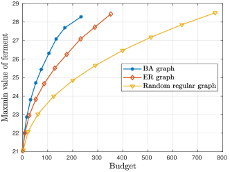
Figure 11: Ferment level attained as a function of the budget in maxmin problem for $k$R, ER, and BA networks.

8 Discussion

We considered the control problem of influencing opinion dynamics on a social network to achieve control objectives. Motivated by ‘mindshare’-like objectives of campaigns, we were interested in the opinion levels (states) over the entire control period. We considered two types of problems—a minimum cost problem with constraints on the allowable states in $\{T_{0},\ldots,T\}$ and a maxmin problem with total cost constraint.

Several open questions remain even within the problem space that we considered. Our extensive simulations indicate that the set of controlled nodes obtained as a solution to the convex relaxation (24) for both TF and GF is submodular. If this were the case then the greedy heuristic is within $(1-1/e)$ of the optimal value. Also, Algorithm 3 that determines the control function for the maxmin problem has numerical stability issues. An algorithm without this deficiency is desirable.

There are of course several variations possible both on the opinion dynamics, and on the state constraints. We expect that the key techniques and the results would be along similar lines. An important class of problems would be to consider multiple opposing campaigns possibly with different control nodes. For example, in [16], we have considered two opposing campaigns in a continuous time $SI_{1}SI_{2}S$ epidemic model and obtained the Nash control strategies. There are of course myriad possibilities.

Appendix A Appendix - Proofs

A.1 Proof of Lemma 4.2

Consider the system

$$\text{minimize}~{}~{}\|u^{e}\|_{2}^{2}$$ (45)

$$\text{subject to }\begin{cases}&x^{e}=Ax^{e}+Bu^{e}+(I_{n}-A)q\\ &x^{e}\geq\tau.\end{cases}$$ (46)

Rewrite (46) as

$$(I_{n}-A)(x^{e}-q) =Bu^{e},$$ (47)

$$x^{e} \geq\tau.$$ (48)

After a change of variable, $(x^{e}-q)\to x^{e}$, we get

$$(I_{n}-A)x^{e} =Bu^{e},$$ (49)

$$x^{e} \geq\tau-q.$$ (50)

We will now focus on the matrix $(I_{n}-A)$ and its inverse. See that since $A$ is substochastic, $(I_{n}-A)^{-1}=\sum_{i=0}^{\infty}A^{i}$. Since all the entries of $A^{i}$ are non-negative for all $i\in\{0,\cdots,\infty\}$, $(I_{n}-A)^{-1}$ has all entries non-negative. That is:

$$(I_{n}-A)^{-1}\succcurlyeq 0.$$ (51)

Now consider the following:

$$x^{e} =(I_{n}-A)^{-1}Bu^{e},$$ (52)

$$x^{e} \geq\tau-q.$$ (53)

Let the set of controlled nodes be $C.$ Here, we have that $Bu^{e}\in\mathbb{R}^{n\times 1}$ has the $k$-th entry non-zero for all $k\in C.$ Let the non-zero entries of $Bu^{e}$ be $c_{k}>0$ for all $k\in C.$ Denote the $l$-th column of matrix $M$ by $M_{l}.$ Now, the constraints can be written as:

$$x^{e} =\sum_{k\in C}c_{k}[(I_{n}-A)^{-1}]_{k}$$ (54)

$$x^{e} \geq\tau-q.$$ (55)

Since $A$ is sub-stochastic, we have $(I_{n}-A)^{-1}=\sum_{i=0}^{\infty}A^{i}.$ Now the original problem can be re-stated as:

$$\text{minimize}~{}~{}~{}\sum_{k\in C}c_{k}^{2}$$ (56)

$$\text{subject to }~{}\sum_{k\in C}c_{k}\left[\sum_{i=0}^{\infty}A^{i}\right]_{k}\geq\tau-q.$$ (57)

It follows from (51) that the above problem has a solution if for all rows of $\sum_{i=0}^{\infty}A^{i}$ there is a non-zero entry in at least one of the columns indexed $k$ for $k\in C$. This is ensured by Assumption 3.

A.2 Proof of (38)

Here we give a proof that when at time $t=t_{3},$ $r(t_{3})=\psi(x(t_{3})),$ the directional derivatives in direction $v$ are equal to (38). From (37), we have

$$\mathcal{D}_{v}H(\lambda,\cdot,\cdot,y,u)(xr)$$

$$=\lim_{\theta\downarrow 0}\frac{H(x+\theta v_{x},r+\theta v_{r},y,u)-H(x,r,y,u)}{\theta}$$

$$=\lim_{\theta\downarrow 0}\frac{\lambda_{x}^{\intercal}(t_{3})A(x(t_{3})+\theta v_{x}-x(t_{3}))}{\theta}$$

$$+\lim_{\theta\downarrow 0}\frac{\lambda_{r}(t_{3})(\text{min}\{\psi(x(t_{3})+\theta v_{x}),r(t_{3})+\theta v_{r}\}-r(t_{3}))}{\theta}$$

$$=\lambda_{x}^{\intercal}(t_{3})Av_{x}+\lambda_{r}(t_{3})\min\left\{\left<\frac{d}{dx}\psi(x(t_{3})),v_{x}\right>,v_{r}\right\}.$$

References

- [1] D. Acemoglu, G. Como, F. Fagnani, and A. Ozdaglar. Opinion fluctuations and disagreement in social networks. Mathematics of Operations Research, 38:1–27, 2013.
- [2] D. Acemoglu and A. Ozdaglar. Opinion dynamics and learning in social networks. Dynamic Games and Applications, 1(1):3–49, March 2011.
- [3] D. Acemoglu, A. Ozdaglar, and A. ParandehGheibi. Spread of (mis)information in social networks. Games and Economic Behavior, 70:194–228, 2010.
- [4] Joel A E Andersson, Joris Gillis, Greg Horn, James B Rawlings, and Moritz Diehl. CasADi—A software framework for nonlinear optimization and optimal control. Mathematical Programming Computation, In Press, 2018.
- [5] M. Azzimonti and M. Fernandes. Social media networks, fake news, and polarization. Technical Report Working Paper 24462, National Bureau of Economic Research, March 2018.
- [6] Albert-László Barabási and Réka Albert. Emergence of scaling in random networks. Science, 286(5439):509–512, 1999.
- [7] Vladimir G. Boltyanski and Alexander S. Poznyak. Robust Maximum Principle” Theory and Applications. Birkhasuer, 2012.
- [8] V. S. Borkar and A. Karnik. Controlled gossip. In Proceedings of the Allerton Conference on Communication, Control, and Computing, 2011.
- [9] V. S. Borkar, J. Nair, and N. Sanketh. Manufacturing consent. IEEE Transactions on Automatic Control, 60(1):104–117, January 2015.
- [10] Francis Clarke. Functional analysis, calculus of variations and optimal control, volume 264. Springer Science & Business Media, 2013.
- [11] Robert Dorfman, Paul Anthony Samuelson, and Robert M Solow. Linear Programming and Economic Analysis. Courier Corporation, 1987.
- [12] Paul Erdös and Alfréd Rényi. On random graphs, I. Publicationes Mathematicae (Debrecen), 6:290–297, 1959.
- [13] Soheil Eshghi, Victor Preciado, Saswati Sarkar, Santosh Venkatesh, Qing Zhao, Raissa D’Souza, and Ananthram Swami. Spread, then target, and advertise in waves: Optimal budget allocation across advertising channels. IEEE Transactions on Network Science and Engineering, 2018.
- [14] J. Ghaderi and R. Srikant. Opinion dynamics in social networks with stubborn agents: Equilibrium and convergence rate. Automatica, 50(12):3209–3215, December 2014.
- [15] Mohak Goyal, Debasish Chatterjee, Nikhil Karamchandani, and D Manjunath. Maintaining ferment. In 2019 IEEE 58th Conference on Decision and Control (CDC), pages 5217–5222. IEEE, 2019.
- [16] Mohak Goyal and D Manjunath. Opinion control competition in a social network. In 2020 International Conference on COMmunication Systems & NETworkS (COMSNETS), pages 306–313. IEEE, 2020.
- [17] Lars Grüne. Economic receding horizon control without terminal constraints. Automatica, 49(3):725–734, 2013.
- [18] Lars Grüne and Roberto Guglielmi. Turnpike properties and strict dissipativity for discrete time linear quadratic optimal control problems. SIAM Journal on Control and Optimization, 56(2):1282–1302, 2018.
- [19] Lars Grüne and Matthias A Müller. On the relation between strict dissipativity and turnpike properties. Systems & Control Letters, 90:45–53, 2016.
- [20] Dorit S Hochbaum and David B Shmoys. A best possible heuristic for the -center problem. Mathematics of Operations Research, 10(2):180–184, 1985.
- [21] A. Jadbabaie, N. Moolavi, A. Sandroni, and A. Tahbaz-Salehi. Non Bayesian social learning. Games and Economic Behavior, 76:210–225, 2012.
- [22] K. Kandhway and J. Kuri. How to run a campaign: Optimal control of SIS and SIR information epidemics. Applied Mathematics and Computation, 231:79–92, 2014.
- [23] K. Kandhway and J. Kuri. Campaigning in heterogenous social networks: Optimal control of SI information epidemics. IEEE/ACM Transactions on Networking, 24(1):383–396, 2016.
- [24] Shruti Kotpalliwar, Pradyumna Paruchuri, Debasish Chatterjee, and Ravi Banavar. Discrete time optimal control with frequency constraints for non-smooth systems. Automatica, 107:493–501, 2019.
- [25] N. Masuda. Opinion control in complex networks. New Journal of Physics, 17(033301), 2015.
- [26] Pradyumna Paruchuri and Debasish Chatterjee. Discrete time Pontryagin maximum principle under state-action-frequency constraints. IEEE Transactions on Automatic Control, 64(10):4202–4208, October 2019.
- [27] M. Pirani and S. Sundaram. On the smallest eigenvalue of grounded Laplacian matrices. IEEE Transactions on Automatic Control, 61(2):509–514, February 2016.
- [28] Anton V Proskurnikov and Roberto Tempo. A tutorial on modeling and analysis of dynamic social networks: Part I. Annual Reviews in Control, 43:65–79, 2018.
- [29] Anton V Proskurnikov and Roberto Tempo. A tutorial on modeling and analysis of dynamic social networks: Part II. Annual Reviews in Control, 45:166–190, 2018.
- [30] Halsey Lawrence Royden. Real analysis. Krishna Prakashan Media, 1968.
- [31] Robert Tibshirani. Regression shrinkage and selection via the LASSO. Journal of the Royal Statistical Society: Series B (Methodological), 58(1):267–288, 1996.
- [32] Emmanuel Trélat. Optimal control and applications to aerospace: Some results and challenges. Journal of Optimization Theory and Applications, 154(3):713–758, 2012.
- [33] John Von Neumann. A model of general economic equilibrium. In Readings in the Theory of Growth, pages 1–9. Springer, 1971.
- [34] W. W. Zachary. An information flow model for conflict and fission in small groups. J. of Anthropological Research, 33(4):pp. 452–473, 1977.