Assessing effect heterogeneity of a randomized treatment using conditional inference trees

Abstract

Treatment effect heterogeneity occurs when individual characteristics influence the effect of a treatment. We propose a novel approach that combines prognostic score matching and conditional inference trees to characterize effect heterogeneity of a randomized binary treatment. One key feature that distinguishes our method from alternative approaches is that it controls the Type I error rate, i.e., the probability of identifying effect heterogeneity if none exists and retains the underlying subgroups. This feature makes our technique particularly appealing in the context of clinical trials, where there may be significant costs associated with erroneously declaring that effects differ across population subgroups. TEHTrees are able to identify heterogeneous subgroups, characterize the relevant subgroups and estimate the associated treatment effects. We demonstrate the efficacy of the proposed method using a comprehensive simulation study and illustrate our method using a nutrition trial dataset to evaluate effect heterogeneity within a patient population.
Treatment effect heterogeneity; causal effects; conditional inference trees; matching.

1 Introduction

Under mild assumptions, randomized experiments estimate the average causal effect (ACE) of an intervention, also referred to as the average treatment effect (ATE). However, individuals may vary in their response to intervention so that the ATE is a poor representation of some individuals’ expected benefit (or harm) from the intervention, a phenomenon often referred to as treatment effect heterogeneity [1]. For a given intervention, two heterogeneity-related questions arise: 1) Is the effect of the intervention heterogeneous? 2) If the intervention effect is heterogeneous, how does it vary across individuals? Many heterogeneity-focused statistical methods address both questions using a single model or procedure. Traditional approaches to characterizing treatment effect heterogeneity have primarily centered around regression modeling with interaction terms between the treatment and covariates. In such models, interaction terms can be used to assess whether treatment effect heterogeneity exists and also to characterize its magnitude. Alternatively, formal nonparametric tests have been developed to test a null hypothesis of zero average treatment effect for any subpopulation defined by covariates and whether the average treatment effect is identical for all subpopulations [2].

1.1 Existing methods for the identification of treatment effect heterogeneity

A rapidly growing toolkit of flexible machine learning techniques has produced several data-driven methods for characterizing treatment effect heterogeneity [3, 4, 5, 6]. Flexible methods for heterogeneous treatment effect estimation include methods based on random forests [7, 8, 9], the LASSO [10], recursive partitioning [11, 12, 13], boosting [14], Bayesian frameworks [15, 16, 17, 18], combination frameworks [19, 20], a generic machine learning approach [21] and a general class of two-stage algorithms that seek to address concerns about adapting machine learning for effect estimation [22].

While many of the aforementioned techniques have shown impressive abilities to identify heterogeneous subgroups in situations where heterogeneity exists, they are often overly aggressive in identifying treatment effect heterogeneity when, in truth, there is none. Put more simply, most existing procedures for detecting treatment effect heterogeneity do not control Type I error. This lack of control of Type I error is particularly problematic in the context of randomized trials, where false declarations of treatment effect heterogeneity for a therapeutic agent could lead to wasteful follow-up studies and inappropriate off-label use in identified sub-populations. Several recently-proposed approaches have taken initial steps to address this issue: Zhang et al. [23] proposed two new splitting criteria within a CART-like framework to maintain a balance between minimizing error in estimating the treatment effect and maximizing heterogeneity; Watson and Holmes [24] compiled machine learning approaches to formally test for the presence of effect heterogeneity, evaluate the predictive benefits of the machine learning algorithm over a traditional statistical model and exert control over the type I error rate; Foster et al. [12] recommended computing an associated measure of uncertainty for each subgroup to account for the consequences of false discovery and Rigdon et al. [25] introduced a matching plus classification and regression tree (mCART) that reduces the potential for falsely detecting treatment effect heterogeneity. Other approaches (e.g., [8]) have also offered a framework to formally test for the overall effect heterogeneity. However, no flexible, unified framework has yet emerged that combines formal inferential testing for treatment effect heterogeneity with a focus on characterization of subgroups experiencing differential treatment effects.

1.2 Our contribution

In this paper, we propose a novel approach to testing for and characterizing effect heterogeneity of a randomized binary treatment on a continuous outcome, while explicitly controlling the Type I error rate. Our Treatment Effect Heterogeneity Tree (TEHTree) method involves building a conditional inference tree using pairs of individuals matched on the prognostic score [26]. After describing the TEHTree method and providing theoretical motivation for matching based on prognostic scores, we present the results of a substantial simulation study demonstrating TEHTree’s Type I error control (power) in the absence (presence) of effect heterogeneity and compare its performance to other established techniques. This simulation study also evaluates subgroup identification and associated characterization for a unified framework (as in Causal Tree and TEHTree) against a two-stage method, which first generates individual treatment effects from an ensemble framework and then runs the effects through a conditional inference tree to determine subgroups. We also offer a comparison of the real-world performance of the two methods using data from a recent randomized trial in nutrition.

2 Method

2.1 Setup and Notation

Let $\mathbf{Y}=\{Y_{1},\dots,Y_{n}\}$ be a continuous response vector for $k$ subjects randomized to treatment $Z=0$ and $n-k$ subjects randomized to treatment $Z=1$. The treatment assignments for all subjects are denoted by $\mathbf{Z}=\{Z_{1},\dots,Z_{n}\}$. An accompanying $n\times p$-dimensional matrix $\mathbf{X}=\{\mathbf{X}_{1},\dots,\mathbf{X}_{p}\}$ contains the $p$ covariates for each of the $n$ subjects with $\mathbf{X}_{i}=\{X_{i1},\dots,X_{ip}\}$.

In the counterfactual framework, each individual has a pair of counterfactual outcomes $(Y_{0i},Y_{1i})$, where $Y_{1i}$ is the outcome of subject $i$ if assigned to treatment $Z=1$ and $Y_{0i}$ the outcome if assigned to $Z=0$. Hence, every individual has a (counterfactual, causal) treatment effect $Y_{1i}-Y_{0i}$, and the Average Treatment Effect (ATE) is defined as the mean of these within-individual differences, $ATE=E[Y(1)-Y(0)]$ (we have switched to the parenthetical counterfactual notation $Y(Z)$ to denote the observation $Y_{Zi}$ for arbitrary $i$). One of the benefits of randomization is that, under often plausible assumptions, the difference in means of randomized groups $E(Y|Z=1)-E(Y|Z=0)$ estimates the ATE. The Stable Unit Treatment Value Assumption (SUTVA) [27] bundles together two assumptions: 1) the treatment assigned to an individual affects only the outcome for that individual, and 2) there is only one “version” of treatment. In most randomized studies, SUTVA is plausible, a notable exception being studies of infectious diseases in closed populations. The other key assumption is ignorability, i.e., that treatment assignment $Z$ is independent of the counterfactual pair $(Y(0),Y(1))$. While this “no unmeasured confounding” assumption is non-trivial in observational studies, it is satisfied by design in a randomized trial.

The counterfactual framework allows every individual $i$ to experience a different effect of treatment, but because study participants are typically assigned to either $Z=1$ or $Z=0$, these individual-level effects $Y_{1i}-Y_{0i}$ are unobserved. Instead, we can characterize treatment effect heterogeneity in the counterfactual framework by estimating the Conditional Average Treatment Effect [28],

$$CATE(\mathbf{x})=E(Y(1)-Y(0)|\mathbf{X}=\mathbf{x}).$$

Because $Z$ is randomized, ignorability holds within any subset defined by $\mathbf{X}=\mathbf{x}$, and hence $CATE(\mathbf{x})$ can be estimated from $E(\mathbf{Y}|Z=1,\mathbf{X}=\mathbf{x})-E(\mathbf{Y}|Z=0,\mathbf{X}=\mathbf{x})\equiv\mu_{1}(\mathbf{x})-\mu_{0}(\mathbf{x})$. Therefore, the key challenge to characterizing treatment effect heterogeneity in randomized studies is to identify distinct subgroups defined by $\mathbf{X}$ with different CATEs. In the absence of treatment effect heterogeneity, the null hypothesis $H_{0}:CATE(\mathbf{x})=ATE\ \forall\mathbf{x}$ holds. Most methods that seek to characterize how CATEs employ flexible semi- and non-parametric techniques in an attempt to identify regions of heterogeneity, but do not control the Type I error probability. In contrast, our approach embeds a classical parametric regression framework within a flexible tree model, allowing for both explicit control of the Type I error rate and characterization of treatment effect heterogeneity when it exists. The following two sections introduce the matching and conditional inference tree techniques that form the basis of our method.

2.2 Matching

If we observed $Y_{1i}$, $Y_{0i}$, and $\mathbf{X}_{i}$ for all $i$ then standard approaches to characterizing variability in a continuous outcome with respect to covariates could be used to estimate CATEs; for example, we could fit a regression tree using the differences $Y_{1i}-Y_{0i}$ as outcomes and $\mathbf{X}_{i}$ as predictors. However, in most trials an individual’s outcome is observed under only one treatment, and hence $Y_{1i}-Y_{0i}$ is unobserved. So, we propose to impute it by matching each individual $i$ assigned to $Z_{i}=1$ with a “similar” individual $j$ having $Z_{j}=0$ and using $(Y_{i}-Y_{j})$ to approximate $Y_{1i}-Y_{0i}$. If $j$ is an “exact” match for $i$ in the sense that $\mathbf{X}_{i}=\mathbf{X}_{j}$, then we can use $E(Y_{i}-Y_{j}|\mathbf{X}_{i}=\mathbf{x})$ to estimate $CATE(\mathbf{x})$. When the number of covariates $p$ is even moderately large and/or elements of $\mathbf{X}$ are continuous, it will typically be impossible to find exact matches for most individuals. One way of overcoming this problem is by deriving a single measure that characterizes the “distance” between individuals. If two individuals $i$ and $j$ with $Z_{i}=1$ and $Z_{j}=0$ have distance $d_{ij}=d$ between them,

$$E(Y_{i}-Y_{j}|\mathbf{X}_{i}=\mathbf{x},\mathbf{X}_{j}=\mathbf{x}^{\prime},d_{ij}=d,Z_{i}=1,Z_{j}=0)=CATE(\mathbf{x})+\Delta^{0}_{ij}(\mathbf{x},\mathbf{x}^{\prime},d)$$ (1)

(see Appendix A for the short proof). Hence, pairs matched according to $d_{ij}$ can be used to estimate CATEs provided $\Delta^{0}$ is small. Note that, in general, $\Delta^{0}$ may be non-zero even if $d=0$; it is the price paid for reducing the multidimensional vectors $\mathbf{x}$ and $\mathbf{x}^{\prime}$ to the scalar distance $d$.

A number of distance measures for matching have been proposed, some of which we review briefly here. Broadly speaking, these measures can be broken down into three categories according to how they define similarity: based on the distance between covariate vectors (e.g., Mahalanobis distance), based on the probability of being treated (propensity score), and based on the predicted value of the outcome (prognostic score). The propensity score [29, 30] is unhelpful, when treatment is randomized, since by design the covariates are independent of treatment assignment and as a result propensity score matching does not make $\Delta^{0}$ small. Another way of summarizing the similarity between individuals is via the prognostic score [26]. Individuals with similar prognostic scores have similar predicted values of the outcome under treatment $Z=0$ (typically a control condition). Matching on prognostic scores is appealing in our context where the goal is approximate individual causal treatment effects $Y_{1i}-Y_{0i}$. If two individuals $i$ and $j$ with $Z_{i}=1$ and $Z_{j}=0$ have the same prognostic score $\phi(\mathbf{X}_{i})=\phi(\mathbf{X}_{j})=\phi$,

$$E(Y_{i}-Y_{j}\mid\mathbf{X}_{i}=\mathbf{x},\mathbf{X}_{j}=\mathbf{x}^{\prime},\phi,Z_{i}=1,Z_{j}=0)=CATE(\mathbf{x})$$ (2)

(see proof in Appendix A). This result immediately implies that if $d_{ij}=|\phi(\mathbf{X}_{i})-\phi(\mathbf{X}_{j})|=0$, then $\Delta^{0}=0$ in Equation 1. In other words, matching on the prognostic score yields pairs that can be used to estimate conditional average treatment effects. Note that this result holds if $\mathbf{X}$ is replaced by any measurable function $m(\mathbf{X})$, so that if $m$ captures the way in which $\mathbf{X}$ modifies the effect of treatment, then pairs matched on $\phi(\mathbf{X})$ retain information about effect modification.

2.3 Conditional Inference Trees

With matched pairs in hand that can be used to estimate CATE$(\mathbf{x})$, the next step is to characterize how the CATE varies with $\mathbf{x}$. Our approach uses conditional inference trees, a variant of decision trees which we briefly introduce here.

The most popular and commonly used technique for building decision trees, the Classification and Regression Tree (CART) technique, was introduced by [31] (originally 1984). Because of its interpretability and flexibility, CART has also been incorporated into several methods for assessing treatment effect heterogeneity. For example, the Causal Tree [13] optimizes for heterogeneity in treatment effects and uses a modified mean-squared criterion expression within a CART framework for both splitting and cross-validation. One of CART’s drawbacks is that, because it considers many possible thresholds on all possible variables when searching for an optimal split, it has a tendency to overfit the data on hand and produce overly complex models. This overfitting tendency can be controlled somewhat by “pruning” trees based on a complexity parameter. However, as we show in our simulation study, even pruned CARTs do not control the Type I error for effect heterogeneity. Several related methods have demonstrated excellent performance in detecting the presence or absence of underlying treatment effect heterogeneity and estimating individual-level CATEs. For example, the Causal Forest algorithm [8], which was developed as an ensemble over Causal Trees, offers an associated formal test for the presence of effect heterogeneity and can estimate $CATE(\mathbf{x})$ for a wide variety of functional relationships between $\mathbf{x}$ and the treatment effect. However, this and similar ensemble methods do not generally yield an interpretable set of subgroups characterizing effect heterogeneity; we highlight these differences in characterization in our simulation study in Section 3.

One alternative to a CART framework is the Conditional Inference Tree (CTree), proposed by [32]. The main difference between CTrees and CARTs is in the splitting process: in CTrees, the processes for choosing a variable to split on or to stop splitting (the “variable selection” step) and choosing an optimal splitting threshold for the selected variable (the “splitting” step) occur sequentially, while in CART they happen simultaneously. In the variable selection step of CTree, the decision of whether not to continue splitting is based on a test of the global null hypothesis $H_{0}:E(\mathbf{Y}|\mathbf{X})=E(\mathbf{Y})$, which is tested by considering all marginal null hypotheses $H_{0}^{m}:E(\mathbf{Y}|\mathbf{X}_{m})=E(\mathbf{Y})$ for $m=1,\dots,p$. In a simple case, each $H_{0}^{m}$ can be assessed by calculating the p-value for the slope term from a univariate regression model of $\mathbf{Y}$ on $\mathbf{X}_{m}$. More generally, this step can accommodate a wide variety of models and test statistics; even if a statistic’s sampling distribution is unknown, permutation tests can be used to calculate p-values for each partial null hypothesis.

Since the global null $H_{0}=\bigcap_{m=1}^{p}H_{0}^{m}$ is rejected if the minimum p-value for all of the partial null hypotheses is less than a pre-specified level of significance, control of Type I error can be achieved by setting this level using an appropriate multiplicity adjustment to account for the testing of the $p$ partial null hypotheses (see Section 2.4.3). If the minimum p-value exceeds the threshold, the tree does not split the given subset further. Otherwise, the partial null hypothesis $H_{0}^{s}$ that results in the smallest p-value will indicate the covariate $\mathbf{X}_{s}$ that is most strongly associated with the outcome $\mathbf{Y}$ and the algorithm proceeds to the next step to determine how to optimally threshold $\mathbf{X}_{s}$. In our method, we calculate p-values associated with the (fixed) slope term from univariate linear mixed models. Once covariate $\mathbf{X}_{s}$ has been selected for splitting, the second step of the CTree algorithm is to find the threshold $c$ that maximizes the discrepancy $|E(\mathbf{Y}|\mathbf{X}_{s}\leq c)-E(\mathbf{Y}|\mathbf{X}_{s}>c)|$. This two-phase splitting procedure is repeated on the resulting partitions until no more subsets are eligible for splitting.

2.4 Treatment Effect Heterogeneity Trees (TEHTrees)

We propose a two-stage approach to assessing treatment effect heterogeneity in randomized studies. In the first stage, prognostic scores are calculated and every treated subject is matched to a control subject (with replacement) based on the prognostic score. In the second stage, within-pair differences in the outcome along with the covariate values of the treated member of each pair are used as inputs to a conditional inference tree. The nodes of the fitted conditional inference tree identify subgroups across which the causal effect of treatment varies. The full algorithm is as follows; in the sections that follow, we provide details about its key steps.

2.4.1 TEHTree algorithm

1. Separate the dataset into a training and holdout set for the purpose of constructing a tree (steps 2-5 below) and for estimating treatment effects (step 6).

2. Fit a model to calculate prognostic scores $\phi$ using individuals in the training data with treatment status $Z=0$, and obtain estimated prognostic scores $\hat{\phi}$ for each individual in the sample. Model details for prognostic score estimation are provided in Section 2.4.2.

3. Form a set of matched pairs $\{(i_{1},j_{1}),(i_{2},j_{2}),\dots,(i_{k},j_{k})\}$ from the training data by matching each treated ($Z=1$) subject with one control ($Z=0$) subject, with replacement, based on $\hat{\phi}$. Ties are broken randomly.

4. For each pair $(i_{l},j_{l})$, calculate the within-pair difference in the outcome, $\delta_{l}=Y_{i_{l}}-Y_{j_{l}}$. Each pair can now be viewed as a single “pseudo-individual” represented by the scalar continuous outcome $\delta_{l}$ and the covariate vector $\mathbf{X}_{l}\equiv\mathbf{X}_{i}$.

5. Use the pseudo-individual data $(\delta_{l},\mathbf{X}_{l})$ created in the previous step and the desired Type I error rate as inputs to create a Treatment Effect Heterogeneity Tree (TEHTree), as described in Section 2.4.3.

6. Estimate the treatment effect within each terminal node of the fitted TEHTree as described in Section 2.4.4.

The preceding algorithm assumes that a sufficient amount of data is available to create a holdout test set of sufficient size to accurately estimate treatment effects within subgroups defined by each terminal node. If the sample size is limited, steps 2-6 can be carried out on the entire dataset with a single-sample estimation approach for step 6 as described in Section 2.4.4.

2.4.2 Estimating prognostic scores

To provide robustness against misspecification of the prognostic score model, we apply the Super Learner [33] to estimate the prognostic score $\phi(\mathbf{X})=E(\mathbf{Y}|Z=0,\mathbf{X})$ using data from the untreated ($Z=0$) group. The base learners in our application consist of the sample mean, a linear model (with and without interaction terms), a generalized additive model, a random forest, stepwise regression (with and without interaction terms), and “polymars” (multivariate adaptive polynomial spline regression) as base learners.

2.4.3 Testing partial null hypotheses

Because the outcome values $\delta_{i,j}$ are derived from pairs formed by matching with replacement, inputs to the conditional inference tree are correlated and hence a standard univariate linear regression-based approach to evaluating the partial null hypotheses $\{H^{0}_{m}:E(\mathbf{Y}|\mathbf{X}_{m})=E(\mathbf{Y})\}$ will produce invalid p-values. Instead, we test partial null hypotheses by fitting univariate linear mixed models of the form:

$$E(\delta_{i,j}|X_{im},b_{j})=\beta_{0}+\beta_{1}X_{im}+b_{j}$$ (3)

where $b_{j}\sim N(0,\tau^{2})$ is a random intercept corresponding to the control subject in each pair. Similar models are used to determine the optimal splitting for selected covariate $\mathbf{X}_{s}$, replacing $X_{im}$ in Equation 3 by $\mathbf{1}[X_{is}\geq c]$.

To establish proof of concept for our method, we used the Bonferroni method to adjust the marginal hypothesis test p-values for multiple comparisons, which sets the significance threshold at $\frac{\alpha}{p}$ for desired Type I error rate $\alpha$. Other less conservative adjustment methods could also be applied; see the Discussion for more details.

2.4.4 Treatment effect estimation

We propose a double-sample (test/holdout set) approach to estimating heterogeneous treatment effects using TEHTree that parallels the one used in the Causal Tree method. After having generated the TEHTree based on the training set, we determine the TEHTree terminal node that each individual in the holdout set belongs to. Each terminal node $\mathcal{T}$ consists of the union of two subsets $\mathcal{T}_{1}=\{i:Z_{i}=1,i\in\mathcal{T}\}$ and $\mathcal{T}_{0}=\{i:Z_{i}=0,i\in\mathcal{T}\}$. We compute the treatment effect estimate as $\Delta(\mathcal{T})=\frac{1}{|\mathcal{T}_{1}|}\sum_{\mathcal{T}_{1}}Y_{i}^{te}-\frac{1}{|\mathcal{T}_{0}|}\sum_{\mathcal{T}_{0}}Y_{i}^{te}$, where $Y_{i}^{te}$ refers to outcomes in the test/holdout set. Note that, for a 1:1 randomized treatment, large discrepancies between $|\mathcal{T}_{1}|$ and $|\mathcal{T}_{0}|$ are unlikely, and hence the precision of $\Delta(\mathcal{T})$ will be approximately proportional to $\frac{1}{\sqrt{|\mathcal{T}|}}$.

If limited sample size precludes carving out an independent holdout set from the original data, a straightforward single-sample estimation approach can be used. Let $\mathcal{T}$ denote the set of matched pairs from the data belonging to each terminal node. Then, the single-sample treatment effect estimate is simply $\Delta(\mathcal{T})=\frac{1}{|\mathcal{T}|}\sum_{l\in\mathcal{T}}\delta_{l}$. Estimation of the precision of the single-sample estimate of $\Delta(\mathcal{T})$ is complicated (relative to the double-sample approach) by the need to consider the correlation between matched pairs. In Section 4, we apply this single-sample approach to the data illustration in the presence of a limited sample size.

2.5 Implementation

We implemented TEHTree in R [34] using a modified conditional inference tree framework and relevant functions in the partykit package [35]. Matching was conducted using the Matching package [36], and all linear mixed models were fit using the nlme package [37]. The Super Learner was used to estimate the prognostic score. Code for implementing TEHTree can be found at https://github.com/AshwiniKV/TEHTree. The Causal Tree and Causal Forest were implemented using the causalTree and grf packages [38].

3 Simulation Study

We conducted simulations to evaluate the TEHTree method and compare its performance to other approaches, including several variants of the Causal Tree technique. We evaluated the Type I error, power, and other statistical properties of the techniques for the tree types over different data generating scenarios that are documented in the Appendix (Tables 1 and 2). Factors that were varied over the scenarios include sample size ($N$ = 100, 200, 500, 1000 and 2000), number of covariates, type of covariates (binary and continuous), coefficients, and pairwise correlation among covariates. The treatment variable $Z$ was generated such that $N/2$ subjects received treatment ($Z=1$) and $N/2$ subjects received control ($Z=0$). All results described in this simulation study are based on 1,000 simulations per scenario. Continuous covariates were generated from multivariate normal distributions with mean zero, unit variance, and varying pairwise correlations. Binary covariates were generated as independent Bernoulli$(0.5)$. Continuous outcomes were generated as independent Normal with unit variance and means depending on the scenarios detailed in Appendix B.

3.1 Type I Error

For a case when there is no treatment effect heterogeneity, we will say that a tree-based method for detecting heterogeneity has committed a Type I error when the tree generates more than one terminal node, incorrectly implying that treatment heterogeneity exists. We generated data under two sets of scenarios where there was no treatment effect heterogeneity. In the first set of scenarios, outcomes were generated from a linear model with main effects for treatment and covariates (Model (M1) in the Table 1). In these scenarios, a simple linear model including treatment and covariates correctly specifies the prognostic score; in other words, the SuperLearner ensemble used to estimate the prognostic score contains the correct model. Figure 1(a) displays the Type I error (in logarithmic scale) of TEHTrees and Causal Trees for data simulated under these scenarios. In all cases, the Type I error of TEHTrees is less than the desired 0.05 level, while the Type I error of Causal Trees is greater than 0.05 in every scenario, usually substantially so. As the sample size increases, the Type I error of Causal Trees increases and is approximately 1 at $N=2000$ for all three scenarios; the Type I error of TEHTrees stays roughly constant. In the second set of scenarios, outcomes were generated from a linear model with main effects of treatment and covariates, along with additional effects for thresholded versions of continuous covariates (Model (M2) in the Appendix, Table 1). In these scenarios, the SuperLearner ensemble does not contain the true model. Figure 1(b) displays the Type I error (in logarithmic scale) for these scenarios. The Type I error rate of TEHTrees tends to increase with sample size and is no longer below the desired 0.05 in every scenario. However, the Type I error rate using TEHTrees is still much lower than the Type I error rate using Causal Trees. We note that this is a particularly challenging scenario for an approach based on prognostic score matching; even modest misspecification of the prognostic score could markedly increase the proportion of matched pairs where one individual has $X>0$ and the other has $X\leq 0$, leading to the (erroneous) conclusion that treatment effects are heterogeneous in $X$. When TEHTree is used with with a correctly-specified prognostic score model (purple points and lines), the Type I error rate is once again controlled.

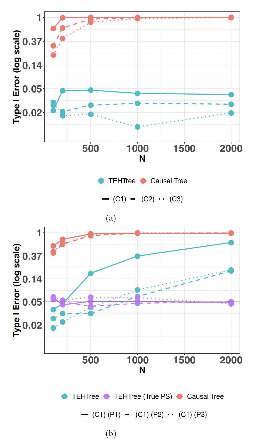
Figure 1: Results of simulations conducted over different scenarios to evaluate the Type I Error rate for TEHTrees and Causal Trees. The plots use data generated from Models M1 and M2, as specified in the Appendix (Table 1). The different scenarios associated with each model and their parameters are also further summarised in the Appendix (Table 2). The error rates are displayed at sample sizes $N$ = 100, 200, 500, 1000 and 2000.

3.2 Power

We characterized the performance of TEHTrees and Causal Trees under a number of different data generating scenarios where treatment effect heterogeneity is driven by binary (dichotomized) covariates only, and a mixture of binary and continuous covariates. We defined the power for detecting treatment effect heterogeneity as the probability that a tree produced a split on a variable having a non-zero interaction with treatment (i.e., one that is responsible for producing treatment effect heterogeneity). Note that while this definition of power does not credit trees with splitting on variables unrelated to heterogeneity, in cases where the treatment effect interacts with several different covariates, a tree is credited with rejecting the null hypothesis if it splits on any of these covariates.

Figures 2(a) through 2(d) summarize the results of scenarios where heterogeneity is determined by a single covariate ($X_{1}$) (Models M3, M4, M5 and M7 in Appendix Table 1), and hence the power is the probability of splitting on $X_{1}$. TEHTrees and Causal Trees have similar power when heterogeneity is determined by $I(X_{1}>0)$ (Figure 2(a)) and by continuous $X_{1}$ (Figure 2(b)); the power of TEHTrees is modestly lower for small sample sizes when both the indicator and continuous value contribute to heterogeneity (Figure 2(c)). TEHTrees and Causal Trees have similar power at higher sample sizes when heterogeneity is induced by $\sin(\eta X_{1})$ (Figure 2(d), at $\eta=1.5$).

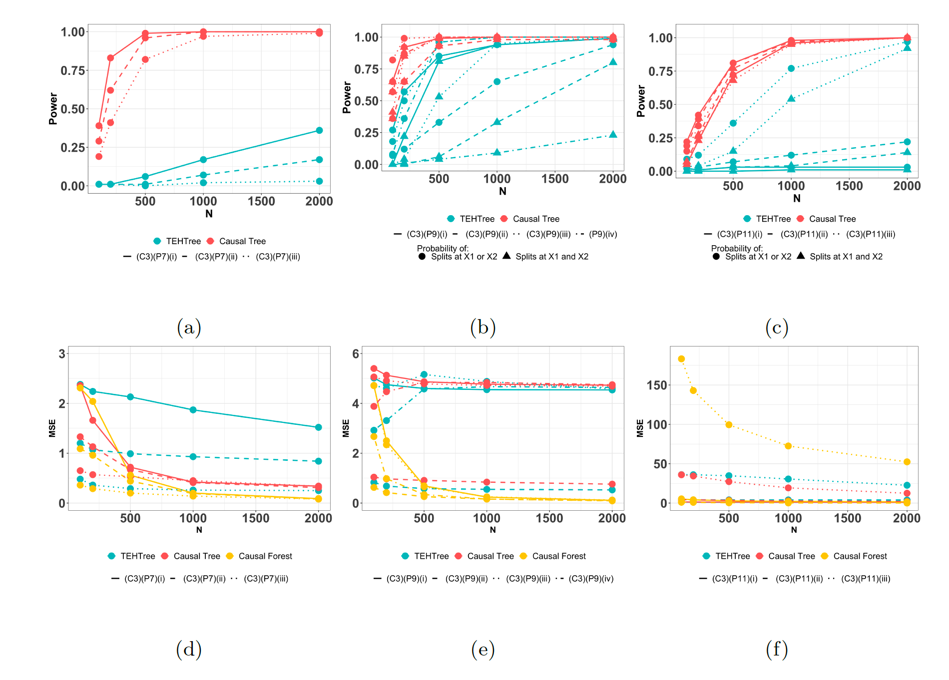
Figure 7: Power (Figure 7(a)-(c)) and Mean-squared error (MSE) (Figure 7(d)-(f)) of the estimated average treatment effect. The data are generated using Models M6, M8 and M10.

Figure 7(a) in the Appendix is notable as it shows that TEHTree has very low power when effect heterogeneity is driven by $I(-0.5<X_{1}<0.5)$. This result is due to the fact that, in our implementation, the null hypothesis $H_{0}:E(\delta_{ij}|X)=E(\delta_{ij})$ is tested via the coefficient of the main effect of $X$ in a (mixed) linear model. When heterogeneity is due to the above indicator, this coefficient will often be estimated as being close to zero and hence the null hypothesis is unlikely to be rejected. An implementation which used a more robust test for variation of the mean with $X$ (e.g., by using a joint test for higher-order polynomial terms) would perform better in this case at the cost of greater computational complexity. As with the utilization of the appropriate functional form and its positive impact on performance, TEHTree is likely to have lower power if important predictor variables are simply not measured.

Figure 2(e) also displays the power of TEHTrees and Causal Trees when heterogeneity in the treatment effect is due to two variables, $X_{1}$ and $X_{2}$. For this Model M9, we considered two definitions of power: splitting on either $X_{1}$ or $X_{2}$, and splitting on both $X_{1}$ and $X_{2}$. In general, both types of power are higher for Causal Trees than TEHTrees.

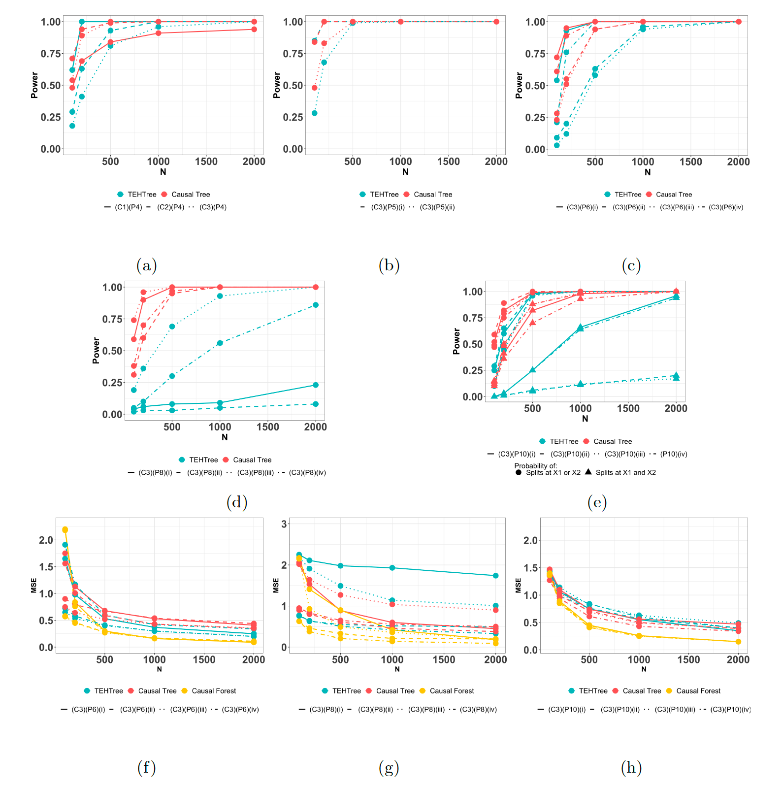
Figure 2: Figures 2(a) - 2(e) present values of power for TEHTrees and Causal Trees. The plots use data generated from Models M3, M4, M5, M7 and M9. Figures 2(f) - 2(h) presents the mean squared error (MSE) of the estimated average treatment effect. The plots use data generated from Models M5, M7 and M9. In both cases, data are generated according to different scenarios with sample sizes N = 100, 200, 500, 1000 and 2000. See Appendix for details of simulation settings and additional results.

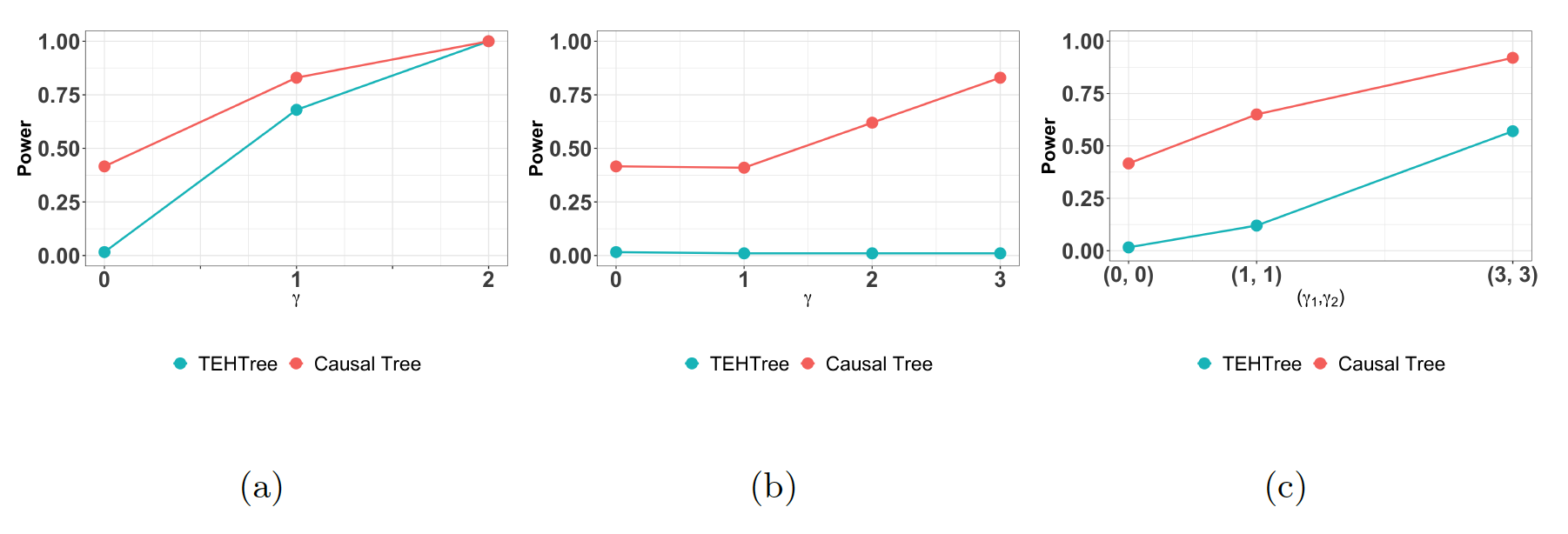
Figure 6: Power of TEHTrees and Causal Trees at different levels of $\gamma$, using scenarios for Models M4, M6 and M8 and when N = 200.

Results for other relevant Models M8 and M10 are available in the Appendix (Figure 7(b)-(c)). While the preceding results show that the Causal Tree approach has higher power than our proposed TEHTree method under many data generating scenarios, this comparison (like most power comparisons) is somewhat misleading since TEHTree controls the Type I error rate while Causal Tree does not. Figure 6 (in the Appendix) shows how the power of Causal Tree and TEHTree vary in Models M4, M6 and M8 as the parameters that determine heterogeneity range from 0 (no heterogeneity) to larger values (substantial heterogeneity).

3.3 Treatment Effect Estimation

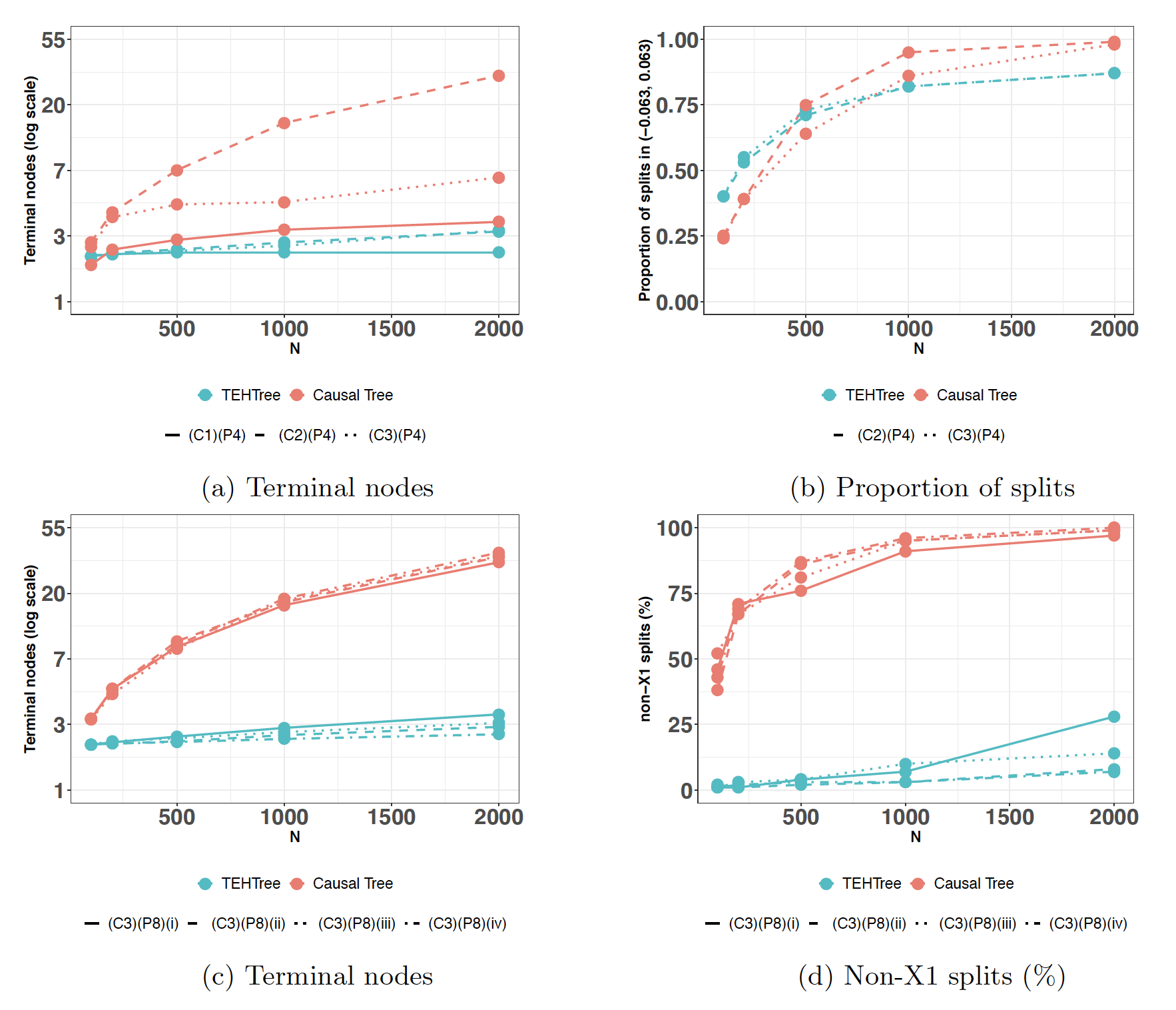
Figure 8: Characteristics of the trees built by TEHTrees (TT) and Causal Trees (CT) when heterogeneity is due to $I(X_{1}>0)$ (in Model M3) and the $\sin(\eta X_{1})$ term (in Model M7). Figure 8(a) and Figure 8(b) correspond to data generated using Model M3 and Figure 8(c) and Figure 8(d) correspond to data generated using Model M7. The described characteristics include the proportion of those split points that are within the middle 5% of a standard normal distribution (i.e., proportion in $I=(-0.063,0.063)$ since the true split point is zero), the average number of terminal nodes (presented in logarithmic scale) when a split is made and proportion of splits at variables besides $\mathbf{X}_{1}$ (presented as a percentage).

Figures 2(f)-(h) present the mean squared error (MSE) of the treatment effect estimates across data generating scenarios and for different sample sizes. The scenarios are defined using Models M5, M7 and M9 and the details are fully described in the Appendix (Tables 1 and 2). Across most scenarios, Causal Trees and TEHTrees show similar MSEs and Causal Forests generally show lower MSEs at larger sample sizes. Characteristics of TEHTrees and Causal Trees using data generated by Model M3 and Model M7 are displayed in the Appendix (Figure 8); the figure describes both the proportion of split points within a given distance of the true split point and the number of terminal nodes.

3.4 Subgroup identification

As demonstrated above, single-method techniques which do not control Type I error tend to ”oversplit” and identify many subgroups when heterogeneity is truly defined by only a few. Figure 3(a) describes these differences in comparison to the Causal Tree and TEHTree algorithms using data generated from Model M1. Across sample sizes, TEHTree retains the Type I error rate control while Causal Forest generated effects leads to trees that continue to split in the absence of effect heterogeneity. Other simulation results for data generated from Models M4, M6, M7 and M8 can be found in the Appendix.

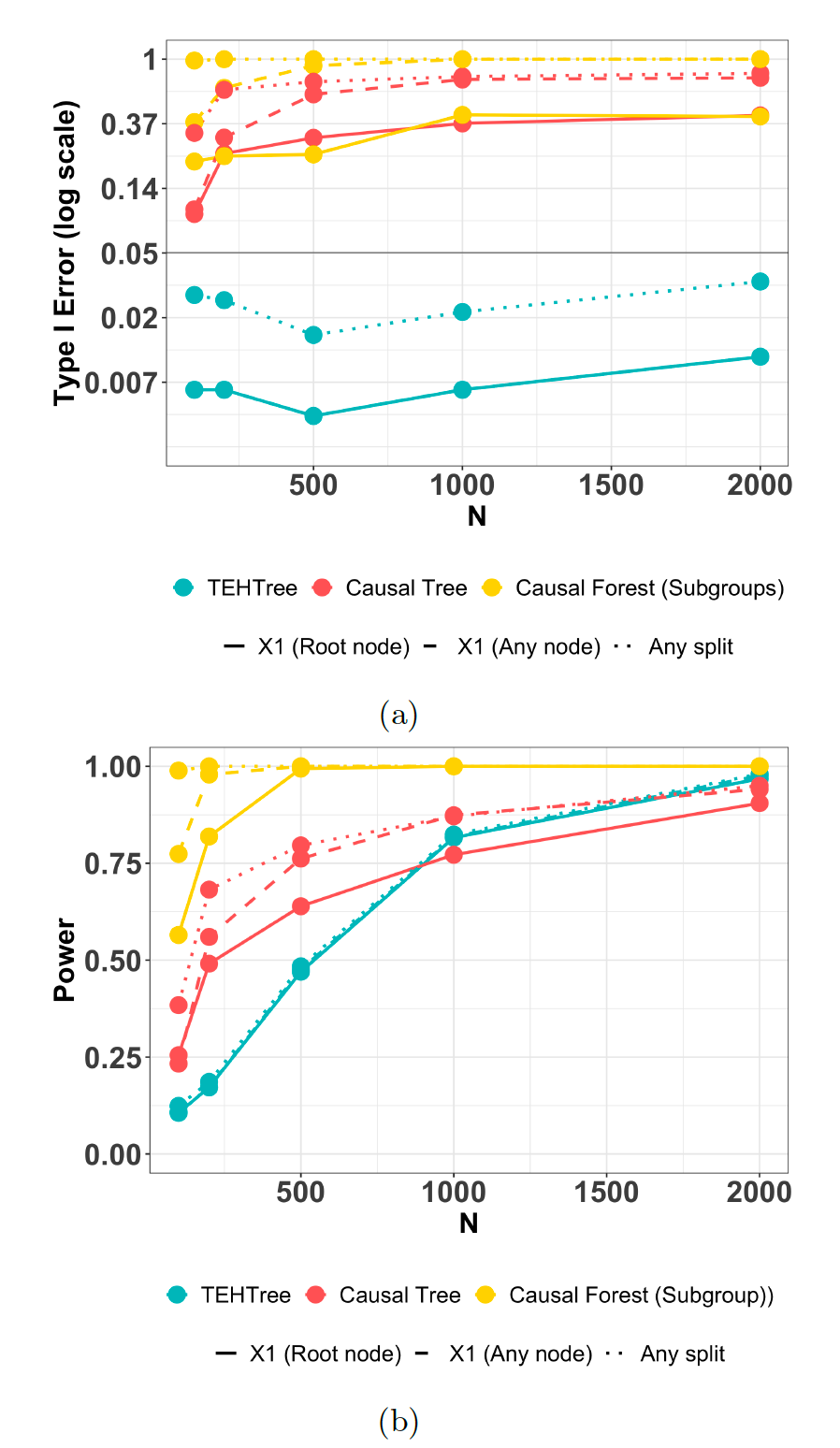
Figure 3: Type I error and Power of different tree types when data are generated over sample sizes N = 100, 200, 500, 1000 and 2000. The data to demonstrate the error rates and power are generated using Models M1 and M3 respectively. For a given simulation, these measures are defined over the probability of the tree splitting at X1 at the root node, the tree splitting at X1 at any node and the probability of a tree splitting at all.

Figure 4 illustrates this phenomenon by showing the sample partitions defined by the terminal nodes of three techniques: TEHTree, Causal Tree, and a decision tree with treatment effects from Causal Forest used as inputs. Each column in the panel corresponds to a tree type and each row is a separate realization of a simulated dataset. In these data, the only driver of effect heterogeneity is $I(X_{1}\geq 0)$, and the methods are given data on two covariates, $X_{1}$ and $X_{2}$. TEHTree consistently identifies the correct subgroups by splitting in the neighborhood of $X_{1}=0$; in four out of five simulated datasets, this is the only split TEHTree produces. The Causal Tree also regularly identifies a split near $X_{1}=0$, but also frequently identifies additional, non-heterogeneity-inducing splits on both $X_{1}$ and $X_{2}$. Treatment effects estimated by Causal Forest are much more heterogeneous, decision trees based on these effects produce multiple splits on both $X_{1}$ and $X_{2}$.

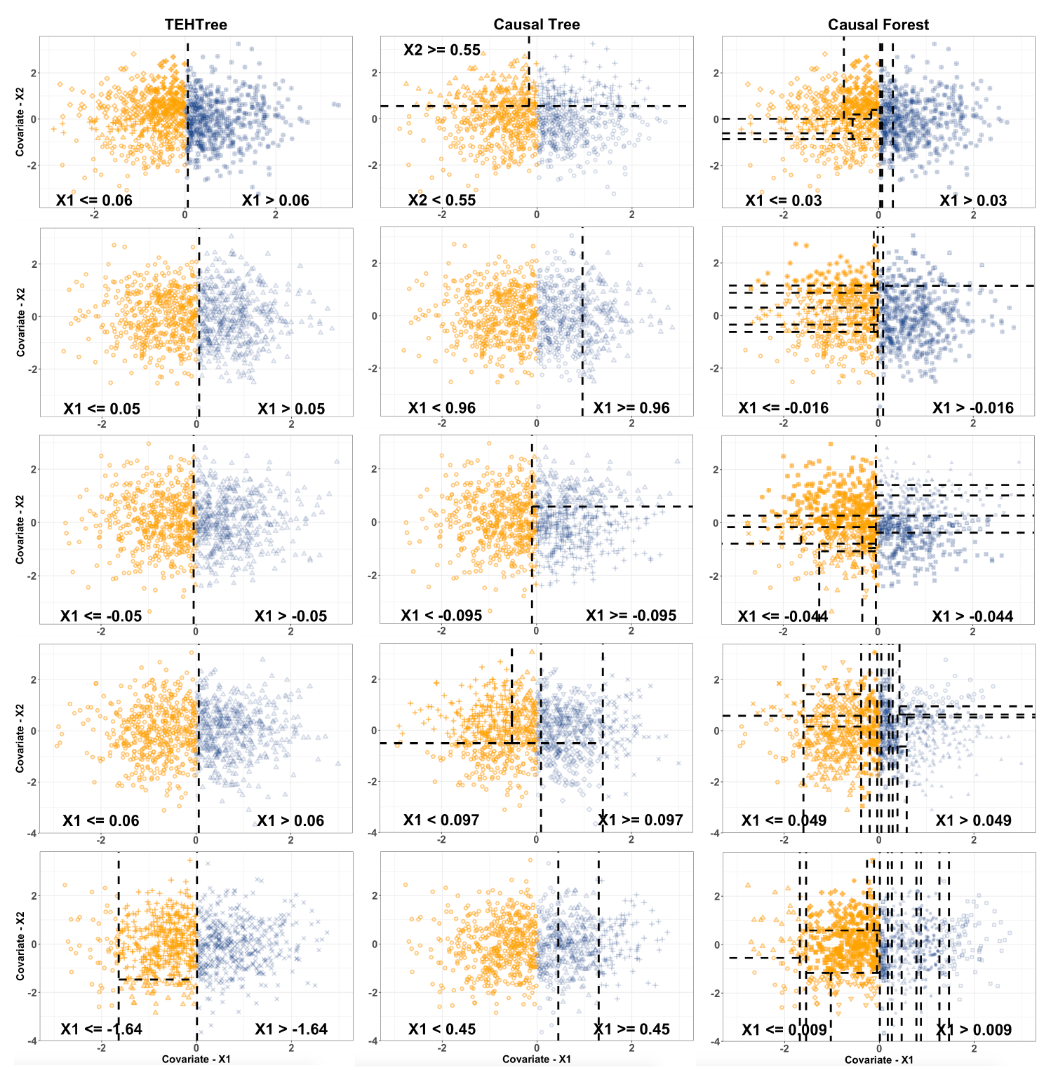
Figure 4: Series of plots showing partitions determined by different tree types (for a continuous outcome, continuous covariates and 1000 corresponding simulated observations using Model M3). The first split at each root node and the criterion is labelled within each plot. Navy blue points within each plot correspond to values where $X_{1}\geq 0$ and orange points correspond to values where $X_{1}<0$. In the first row, the first plot displays partitions for a TEHTree (Root node splits at $X_{1}\leq 0.06$), the second plot for a Causal Tree (Root node splits at $X_{2}\geq 0.55$) and the third plot displays partitions extracted using a Conditional Inference Tree over treatment effects estimated from a Causal Forest (Root node splits at $X_{1}\leq 0.03$). This panel displays partitions determined by three different tree types for five simulated datasets (as corresponding to the five rows and three columns).

4 Illustration

We illustrate the application of TEHTree, Causal Tree, and Causal Forest to data from the Box Lunch Study (BLS) [39], a randomized controlled trial to evaluate the effect of receiving daily boxed lunches of three different portion sizes (400 kcal, 800 kcal, and 1600 kcal) on daily energy intake and body weight of working adults. The BLS study enrolled 233 subjects including a group that did not receive any boxed lunches; we analyzed a complete-case version of the data where 156 subjects were assigned to receive one of the three fixed portion size lunches. More specifically, we consider the problem of characterizing heterogeneity across the effect of “treatment” (defined as the 800 and 1600 kcal boxed lunches, $n=107$) versus “control” (the 400 kcal boxed lunch, $n=49$) on daily caloric intake six months after randomization. The average treatment effect (ATE) is a difference of 193 kcal/day. For this analysis, we consider how the ATE varies with four baseline covariates: BMI, age, a measure of hunger, and EDEQ-14.0, a measure of loss of control over eating in the past 28 days.

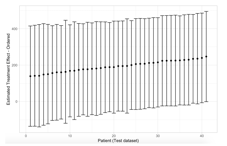
Figure 10: Estimated treatment effects (determined using a Causal Forest algorithm) for patients in the test dataset.

We applied Causal Forest [8] to estimate individual treatment effects and empirically evaluate the presence of effect heterogeneity. The Causal Forest was fit to a training dataset of 117 subjects including the 4 baseline patient characteristics and the relevant causal treatment effects were estimated on 39 test set subjects (displayed in Figure 10 in the Appendix). The results suggest that the subjects experience a relatively homogeneous response to treatment with respect to these covariates. The method does not explicitly identify covariates which induce heterogeneity.

Next, we compared the results of applying TEHTree and Causal Tree to the data. Figures 5(a)-(b) show the TEHTree and Causal Tree that result from analyzing the BLS data. TEHTree was implemented using the modifications specified in Section 2.4.4, and the double-sample Causal Tree method used the default parameters with the exception of setting a minimum size for splitting to 10 treated and 10 controls. While both trees identify covariates that induce heterogeneity, the covariate identified and their split points are quite different. Figures 5(c)-(d) represent the results of applying Causal Tree and TEHTree to a permuted version of the dataset in which the rows of the covariate matrix were permuted to remove associations between covariates and the outcomes but retain within-covariate correlation. In these data, there should be no association between covariates and treatment effects, however, Causal Tree identifies three heterogeneous subgroups defined by age and BMI. TEHTree does not generate any splits, correctly reflecting the true lack of heterogeneity in the permuted data.

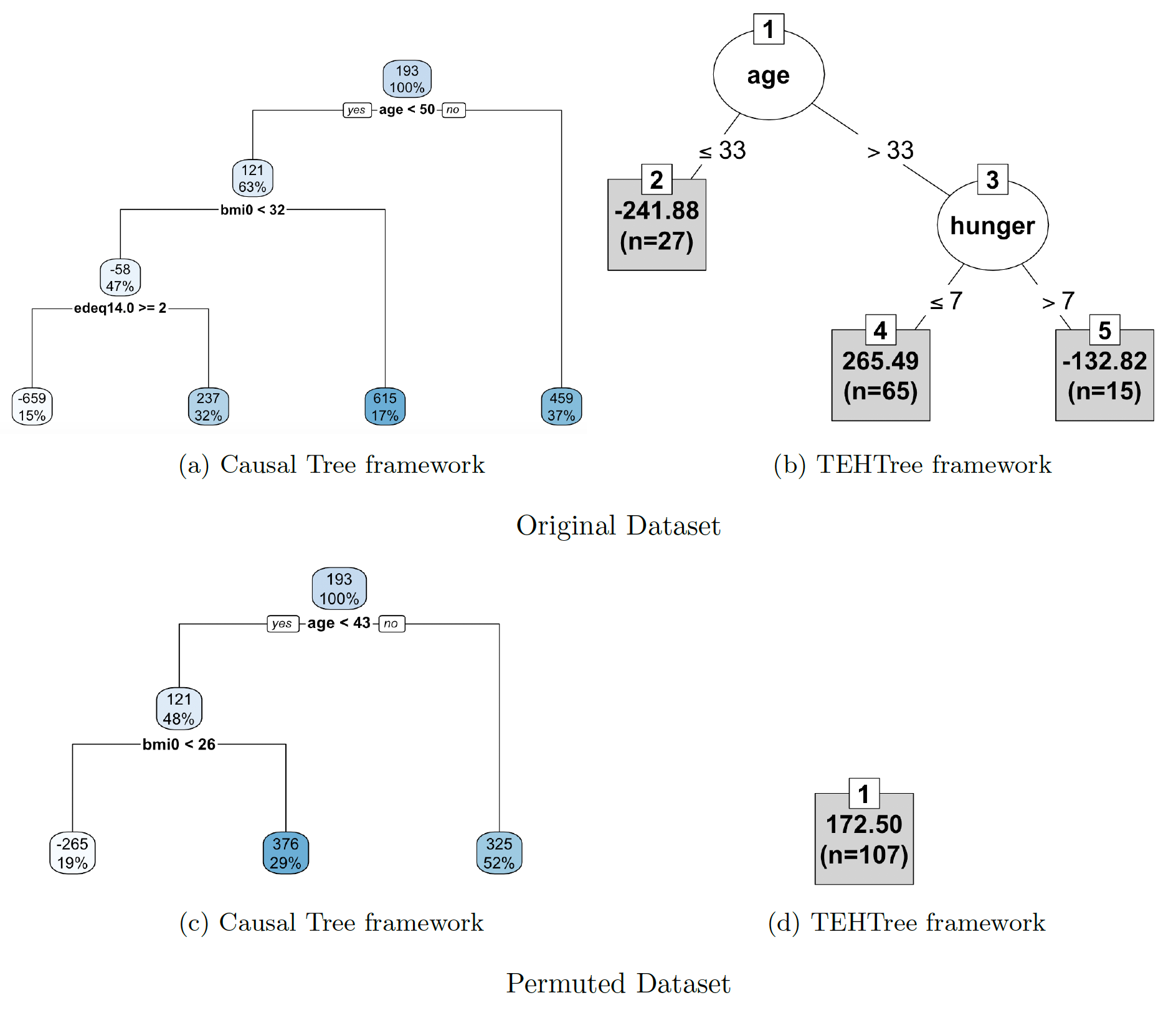
Figure 5: Results of applying Causal Tree and TEHTrees to identify heterogeneity in the effect of the intervention on daily caloric intake using data (with four different covariates) from the Box Lunch Study. Sub-figures 5(a) and 5(b) show the trees produced by applying the methods to the original dataset, and sub-figures 5(c) and 5(d) show the trees when the methods are applied to a dataset where the rows permuted to remove covariate-outcome associations.

5 Discussion

Characterizing treatment effect heterogeneity is becoming a common target of secondary analyses of data from randomized controlled trials. As an alternative to methods that require that the nature of potential subgroups be pre-specified (e.g., via covariate interactions with treatment), several methods have been recently proposed to detect treatment effect heterogeneity in a more data-driven manner [13, 8, 14, 19]. However, while most of these methods incorporate procedures for preventing overfitting, they do not offer any guarantees about Type I error, i.e., the probability of identifying heterogeneous subgroups in the absence of treatment effect heterogeneity. Particularly in the context of randomized trials, explicit control of Type I error may increase the willingness of researchers to apply treatment effect heterogeneity techniques. In this paper, we propose TEHTrees, a novel method that uses a conditional inference tree framework to characterize effect heterogeneity of a binary treatment while controlling the Type I error rate.

As shown in our simulation study, existing methods often yield much higher than nominal Type I error rates, with this error rate generally increasing with sample size. In contrast, TEHTree maintains the specified Type I error rate across most scenarios. In some scenarios, the power of TEHTrees to detect true heterogeneity is competitive with Causal Tree; in other scenarios, TEHTrees has lower power, but these discrepancies mostly arise in scenarios where Causal Tree has very high Type I error rates, i.e., its power curve lies above that of TEHTrees for both null and alternative hypotheses. Causal Trees displayed lower MSE than TEHTrees in multiple scenarios, which was most likely due to greater variability in split points for TEHTree structures. We conjecture that this variability can be attributed to the bias introduced by the matching estimator. Decreasing bias in the matching estimator, or using an alternative approach to estimating the outcomes that are used as inputs in the conditional inference tree of TEHTrees, may improve estimation of treatment effects with TEHTrees when there are continuous covariates.

TEHTrees offer a flexible approach to detecting effect heterogeneity, and its various building blocks allow for numerous modifications including the choice of a different matching algorithm, an alternative prognostic score model, the utilisation of other criteria to select the splitting variable or its split point, or the implementation of a different estimation technique. For example, the Bonferroni correction method used to find the splitting variable in TEHTrees is likely too conservative to detect small treatment effects when there are a large number of covariates in the study. Alternative multiple comparison adjustment methods should be explored in such cases, e.g., controlling the false discovery rate may be a desirable alternative. In addition, the TEHTree approach could be modified to use other regression models for determining splitting variables; indeed, any technique that tests the relevant marginal null hypotheses while accounting for the matching-induced correlation could be easily incorporated in the TEHTree framework. Our method also inherits the desirable properties of conditional inference trees including the fact that unlike the CART-based Causal Tree, TEHTrees do not favor the inclusion of continuous variables with many potential split points over categorical variables with fewer [40].

Other modifications and extensions could also improve the robustness of TEHTrees. Like many matching-based approaches, our method does not account for the variability introduced by the matching estimator, so an extra step may be required to control for the inflation of Type I error that might occur in situations when good matches are difficult to obtain due to lack of overlap in covariate distributions between treatment groups. However, in randomized studies covariates are, on average, balanced between treatment groups and hence lack of overlap between the supports of the covariate distributions is unlikely to be a problem. TEHTree’s performance depends on the accuracy of the prognostic score model. As shown in the simulation, using an ensemble approach to estimating the prognostic score provides a degree of (but not total) robustness against prognostic score misspecification. One type of misspecification that we did not consider in the simulation was omission of predictors of the outcome; as with most matching-based methods, omission of such variables will decrease the quality of the resulting matches and hence lead to poorer performance.

Though we assume treatment is randomized throughout this paper, TEHTrees could be extended for use with observational data involving non-randomized treatments or exposures. However, additional assumptions and modifications to the method would be required to achieve covariate balance and ensure unbiased estimation of treatment effects.

Appendix A

A.1 Appendix A: Proofs

Proof of Equation 1

$$E(Y_{i}-Y_{j}|\mathbf{X}_{i} = \mathbf{x},\mathbf{X}_{j}=\mathbf{x}^{\prime},d_{ij}=d,Z_{i}=1,Z_{j}=0)$$

$$= E(Y_{1i}-Y_{0j}|\mathbf{X}_{i}=\mathbf{x},\mathbf{X}_{j}=\mathbf{x}^{\prime},d_{ij}=d)$$

$$= E(Y_{1i}-Y_{0i}|\mathbf{X}_{i}=\mathbf{x},d_{ij}=d)+E(Y_{0i}-Y_{0j}|\mathbf{X}_{i}=\mathbf{x},\mathbf{X}_{j}=\mathbf{x}^{\prime},d_{ij}=d)$$

$$= E(Y_{1i}-Y_{0i}|\mathbf{X}_{i}=\mathbf{x})+\Delta^{0}_{ij}(\mathbf{x},\mathbf{x}^{\prime},d)$$

$$= CATE(\mathbf{x})+\Delta^{0}_{ij}(\mathbf{x},\mathbf{x}^{\prime},d)$$

Proof of Equation 2

$$E(Y_{i}-Y_{j}\mid\mathbf{X}_{i} = \mathbf{x},\mathbf{X}_{j}=\mathbf{x}^{\prime},\phi,Z_{i}=1,Z_{j}=0)$$

$$= E(Y_{1i}-Y_{0j}|\mathbf{X}_{i}=\mathbf{x},\mathbf{X}_{j}=\mathbf{x}^{\prime},\phi)$$

$$= E(Y_{1i}-Y_{0i}|\mathbf{X}_{i}=\mathbf{x},\phi)+E(Y_{0i}-Y_{0j}|\mathbf{X}_{i}=\mathbf{x},\mathbf{X}_{j}=\mathbf{x}^{\prime},\phi)$$

$$= E(Y_{1i}-Y_{0i}|\mathbf{X}_{i}=\mathbf{x})+E({Y}_{0i}-Y_{0j}|\phi)$$

$$= E(Y_{1i}-Y_{0i}|\mathbf{X}_{i}=\mathbf{x})+0=CATE(\mathbf{x})$$

A.2 Appendix B: Simulation Scenarios and Additional Results

Continuous covariates were generated from multivariate normal distributions with mean zero, unit variance, and varying pairwise correlations. Binary covariates were generated as independent Binomial$(1,0.5)$. Continuous outcomes were generated as independent $\mathcal{N}$($\mu,1$) with linear predictor $\mu$ as defined below in Table 1. We set $\alpha$ to 0.8, $\theta$ to 0.8 and $\beta$ to $(1.0,0.8,0.6,0.4,0.2)^{T}$ for the first five covariates (0 otherwise). The following models (M1 - M10) and their relevant parameters are used over multiple data scenarios, where data are simulated over $N$ different sample sizes (i.e., $N=100,200,500,1000$ and $2000$).

Table 1: Simulation parameters

Models	(M1)	$\mu=0.8+0.8Z+\beta\mathbf{X}$
	(M2)	$\mu=0.8+0.8Z+\beta\mathbf{X}+\phi I(\mathbf{X}>0)$
	(M3)	$\mu=0.8+0.8Z+\beta\mathbf{X}+\gamma Z\cdot I(X_{1}>0)$
	(M4)	$\mu=0.8+0.8Z+\beta\mathbf{X}+\gamma Z\cdot X_{1}$
	(M5)	$\mu=0.8+0.8Z+\beta\mathbf{X}+\gamma_{1}Z\cdot X_{1}+\gamma_{2}Z\cdot I(X_{1}>0)$
	(M6)	$\mu=0.8+0.8Z+\beta\mathbf{X}+\gamma Z\cdot I(-0.5<X_{1}<0.5)$
	(M7)	$\mu=0.8+0.8Z+\beta\mathbf{X}+\gamma Z\cdot\sin(\eta X_{1})$
	(M8)	$\mu=0.8+0.8Z+\beta\mathbf{X}+\gamma_{1}Z\cdot I(X_{1}>0)+\gamma_{2}Z\cdot I(X_{2}>0))$
	(M9)	$\mu=0.8+0.8Z+\beta\mathbf{X}+\gamma_{1}Z\cdot X_{1}+\gamma_{2}Z\cdot I(X_{2}>0)$
	(M10)	$\mu=0.8+0.8Z+\beta\mathbf{X}+\gamma Z\cdot\mathbf{X}$
	(M11)	$\mu=0.8+0.8Z+\beta\mathbf{X}+\gamma_{1}Z\cdot\mathbf{X}_{C}+\gamma_{2}Z\cdot\mathbf{X}_{B}$
		$\beta=(1.0,0.8,0.6,0.4,0.2,0,\dots,0)^{T}$
Covariates	(C1)	$\mathbf{X}$ = 5 independent binary covariates
	(C2)	$\mathbf{X}$ = 5 independent continuous covariates
	(C3)	$\mathbf{X}$ = 10 independent continuous covariates
Coefficients	(P1)	$\phi_{1}=3,\phi_{2}=\phi_{3}=\phi_{4}=\phi_{5}=0$
	(P2)	$\phi_{1}=1,\phi_{2}=\phi_{3}=\phi_{4}=\phi_{5}=0$
	(P3)	$\phi_{1}=\phi_{2}=1,\phi_{3}=\phi_{4}=\phi_{5}=0$
	(P4)	$\gamma=1$
	(P5)	(i) $\gamma=2$, (ii) $\gamma=1$
	(P6)	(i) $\gamma_{1}=\gamma_{2}=1$, (ii) $\gamma_{1}=1,\gamma_{2}=-1$,
		(iii) $\gamma_{1}=-1,\gamma_{2}=1$, (iv) $\gamma_{1}=\gamma_{2}=-1$
	(P7)	(i) $\gamma=3$, (ii) $\gamma=2$, (iii) $\gamma=1$
	(P8)	(i) $\gamma=2,\eta=2$, (ii) $\gamma=1,\eta=2$,
		(iii) $\gamma=2,\eta=1.5$, (iv) $\gamma=1,\eta=1.5$
	(P9)	(i) $\gamma_{1}=3,\gamma_{2}=3$, (ii) $\gamma_{1}=1,\gamma_{2}=1$,
		(iii) $\gamma_{1}=3,\gamma_{2}=-3$, (iv) $\gamma_{1}=1,\gamma_{2}-3$
	(P10)	(i) $\gamma_{1}=\gamma_{2}=1$, (ii) $\gamma_{1}=1,\gamma_{2}=-1$,
		(iii) $\gamma_{1}=-1,\gamma_{2}=1$, (iv) $\gamma_{1}=\gamma_{2}=-1$
	(P11)	(i) $\gamma=1$, (ii) $\gamma=2$, (iii) $\gamma=6$

Table 2: Simulation scenarios corresponding to main figures. Scenario codes are fully described in Table 1.

Evaluating Type I Error
Figure 1(a)
(M1) (C1)-(C3)	Correctly specified prognostic score
Figure 1(b)
(M2) (C1) (P1)-(P3)	Incorrectly specified prognostic score
Evaluating Power, MSE and Tree Characteristics
Figures 2(a) & 8(a)
(M3) (C1)-(C3) (P4)	Heterogeneity according to $I(X_{1}>0)$
Figure 8(b)	[(i)-(iii) refers to settings (C1)-(C3)]
(M3) (C2)-(C3) (P4)	[(ii)-(iii) refers to settings (C2)-(C3)]
Figure 2(b) & 6(a)
(M4) (C3) (P5) (i)-(ii)	Heterogeneity according to $X_{1}$
Figures 2(c) & 2(f)
(M5) (C3) (P6) (i)-(iv)	Heterogeneity according to $I(X_{1}>0)$ and $X_{1}$
Figures 7(a), 6(b) & 7(d)
(M6) (C3) (P7) (i)-(iii)	Heterogeneity according to $I(-0.5<X_{1}<0.5)$
Figures 2(d) & 2(g)
Figures 8(c) & 8(d)	Heterogeneity according to $\sin(\eta X_{1})$
(M7) (C3) (P8) (i)-(iv)
Figures 7(b), 6(c) & 7(e)
(M8) (C3) (P9) (i)-(iv)	Heterogeneity according to $I(X_{1}>0)$ and $I(X_{2}>0)$
Figures 2(e) & 2(h)
(M9) (C3) (P10) (i)-(iv)	Heterogeneity according to $X_{1}$ and $I(X_{2}>0)$
Figures 7(c) & 7(f)
(M10) (C3) (P11) (i)-(iii)	Heterogeneity according to $X_{1},\dots,X_{10}$
Subgroup Identification
Figure 3
(M1) (C2) & (M3) (C2)	Heterogeneity according to $X_{1}$
Figure 4
(M3) Covariates $X_{1}$ & $X_{2}$	Heterogeneity according to $X_{1}$
Variable Selection
Figure 9
(M11) (C3)	Heterogeneity according to $X_{1}$ and $X_{6}$

Additional scenarios for Models M1 - M10

The results evaluated using Model M1 and Model M2 were displayed in Figures 1(a) and 1(b) using data generated over $N$ = 100, 200, 500, 1000 and 2000. However, the results displayed in Figure 1 assumes the absence of pairwise correlation ($\rho=0$) among the five covariates. Table 3 present results for non-zero values of pairwise correlation $(\rho=0.2,\rho=0.4,\rho=0.6,\rho=0.8)$ over continuous covariates (m = 5) at $N$ = 200 and $N$ = 500. Similarly, Model M2 was varied using different vectors of coefficients for five continous covariates and Table 4 presents results for two additional vectors of coefficients.

Table 3: Type I Error rate when there is no treatment effect heterogeneity (i.e., when $\gamma=0$) and the data are generated according to Model M1. This table presents results for non-zero values of pairwise correlation $(\rho=0.2,\rho=0.4,\rho=0.6,\rho=0.8)$ over continuous covariates (m = 5) at $N$ = 200 and $N$ = 500.

Covariate Type	N	m	$\rho$	Type I Error Rate
				TT	CT
Continuous	200	5	0.2	0.030	0.687
Continuous	200	5	0.4	0.026	0.767
Continuous	200	5	0.6	0.026	0.825
Continuous	200	5	0.8	0.050	0.851
Continuous	500	5	0.2	0.023	0.970
Continuous	500	5	0.4	0.026	0.991
Continuous	500	5	0.6	0.030	0.994
Continuous	500	5	0.8	0.045	0.998

Table 4: Type I Error rate of TEHTrees and Causal Tree when there is no treatment effect heterogeneity and the data are generated according to Model M2. The last column shows the Type I Error of TEHTrees when the true prognostic scores are used in matching.

N	m	$\phi_{1}$	$\phi_{2}$	$\phi_{3}$	$\phi_{4}$	$\phi_{5}$	Type I Error Rate
							TT	CT	TT (true PS)
100	5	0.5	1	0	0	0	0.024	0.429	0.053
200	5	0.5	1	0	0	0	0.021	0.627	0.052
500	5	0.5	1	0	0	0	0.031	0.904	0.062
1000	5	0.5	1	0	0	0	0.056	0.986	0.048
2000	5	0.5	1	0	0	0	0.155	0.995	0.060
100	5	1	1	1	1	1	0.026	0.433	0.053
200	5	1	1	1	1	1	0.019	0.677	0.046
500	5	1	1	1	1	1	0.032	0.956	0.044
1000	5	1	1	1	1	1	0.092	0.997	0.046
2000	5	1	1	1	1	1	0.144	0.998	0.054

Table 5: Power of TEHTrees and Causal Trees when data are generated according to Model M3 and there is treatment effect heterogeneity.

Covariate Type	N	m	$\rho$	Power
				TT	CT
Continuous	200	5	0.2	0.68	0.93
Continuous	200	5	0.4	0.72	0.89
Continuous	200	5	0.6	0.73	0.88
Continuous	200	5	0.8	0.66	0.83
Continuous	500	5	0.2	0.97	0.98
Continuous	500	5	0.4	0.98	0.98
Continuous	500	5	0.6	0.98	0.95
Continuous	500	5	0.8	0.95	0.94

Table 6: Characteristics of the trees including the median and mean of the first split point on $X_{1}$ (the variable with heterogeneous treatment effects). Data are generated using Model M3.

Covariate	N	m	$\rho$	Median		Mean
type				split point		split point
				TT	CT	TT	CT
Continuous	100	5	0.0	-0.01	-0.01	-0.01	-0.01
Continuous	200	5	0.0	0.00	0.00	0.00	0.00
Continuous	500	5	0.0	0.00	0.00	0.00	0.00
Continuous	1000	5	0.0	0.00	-0.00	0.00	-0.00
Continuous	2000	5	0.0	0.00	-0.00	0.00	-0.00
Continuous	100	10	0.0	-0.01	-0.03	-0.03	-0.02
Continuous	200	10	0.0	0.00	0.01	0.02	0.01
Continuous	500	10	0.0	0.00	0.00	0.00	0.00
Continuous	1000	10	0.0	0.00	0.00	0.00	0.00
Continuous	2000	10	0.0	0.00	0.00	0.00	-0.00
Continuous	200	5	0.2	0.00	0.00	0.00	0.00
Continuous	200	5	0.4	0.00	-0.00	0.00	-0.00
Continuous	200	5	0.6	0.00	0.00	-0.01	-0.00
Continuous	200	5	0.8	0.00	0.00	0.01	-0.01
Continuous	500	5	0.2	0.00	-0.00	0.00	-0.00
Continuous	500	5	0.4	0.00	-0.00	-0.01	-0.00
Continuous	500	5	0.6	-0.01	-0.00	0.00	-0.00
Continuous	500	5	0.8	-0.01	-0.00	-0.01	-0.01

Table 7: Power and MSE of the estimated average treatment effect for TEHTrees (TT) and Causal Tree (CT) when data are generated according to Model M4. Power is defined to be the probability of the tree making a split on $X_{1}$. MSE is also computed for Causal Forests (CF) using the estimated individual treatment effects against the generated ‘true’ treatment effects.

$\gamma$	N	$\rho$	Power		# nodes		% non-$X_{1}$ split		MSE
			TT	CT	TT	CT	TT	CT	TT	CT	CF
1	200	0.2	0.70	0.83	2.15	5.09	0.05	0.87	0.89	1.22	0.64
1	500	0.2	0.99	0.99	2.90	11.53	0.09	0.99	0.50	0.80	0.27
1	200	0.4	0.76	0.80	2.20	5.18	0.09	0.90	0.93	1.28	0.58
1	500	0.4	1.00	0.98	2.99	11.60	0.13	0.99	0.52	0.85	0.26
1	200	0.6	0.74	0.76	2.25	5.22	0.17	0.91	0.97	1.26	0.51
1	500	0.6	0.99	0.96	3.10	11.11	0.19	0.97	0.51	0.82	0.24
1	200	0.8	0.64	0.71	2.24	5.21	0.29	0.89	1.01	1.09	0.43
1	500	0.8	0.96	0.93	3.20	10.88	0.33	0.96	0.52	0.70	0.20

Table 8: Power and MSE of the estimated average treatment effect for TEHTrees (TT) and Causal Tree (CT) when data are generated according to Model M5. Power is defined to be the probability of the tree making a split on $X_{1}$. MSE is also computed for Causal Forests (CF) using the estimated individual treatment effects against the generated ‘true’ treatment effects.

$\gamma_{1}$	$\gamma_{2}$	N	$\rho$	Power		# nodes		% non-$X_{1}$ split		MSE
				TT	CT	TT	CT	TT	CT	TT	CT	CF
-1	-1	200	0.2	0.82	0.95	2.14	4.42	0.06	0.68	1.14	1.04
-1	-1	500	0.2	1.00	1.00	2.71	10.46	0.15	0.92	0.59	0.69
-1	-1	200	0.4	0.81	0.98	2.19	4.95	0.13	0.82	1.16	1.06
-1	-1	500	0.4	1.00	1.00	2.88	11.36	0.29	0.99	0.59	0.70
-1	-1	200	0.6	0.81	0.96	2.26	5.03	0.23	0.86	1.14	1.04
-1	-1	500	0.6	1.00	1.00	3.16	11.32	0.44	0.98	0.58	0.66
-1	-1	200	0.8	0.68	0.93	2.37	5.03	0.42	0.91	1.09	0.92
-1	-1	500	0.8	0.96	1.00	3.44	11.01	0.60	0.98	0.57	0.59

Table 9: Power and MSE of the estimated average treatment effect for TEHTrees and Causal Tree when data are generated according to Model M6. Power is defined to be the probability of the tree making a split on $X_{1}$. MSE is also computed for Causal Forests (CF) using the estimated individual treatment effects against the generated ‘true’ treatment effects.

$\gamma$	N	$\rho$	Power		# nodes		% non-$X_{1}$ split		N	MSE
			TT	CT	TT	CT	TT	CT		TT	CT	CF
3	200	0.2	0.13	1.00	2.88	19.59	0.17	0.99	1000	1.97	0.57	0.20
3	500	0.2	0.31	1.00	3.48	38.13	0.40	1.00	2000	1.64	0.43	0.09
3	200	0.4	0.13	1.00	2.83	21.14	0.21	1.00	1000	1.98	0.60	0.19
3	500	0.4	0.35	1.00	3.60	38.00	0.47	1.00	2000	1.66	0.42	0.09
3	200	0.6	0.15	0.99	2.85	20.30	0.28	0.99	1000	1.97	0.58	0.18
3	500	0.6	0.36	1.00	3.63	36.76	0.53	1.00	2000	1.70	0.39	0.09
3	200	0.8	0.17	0.98	2.97	19.36	0.32	0.98	1000	1.97	0.54	0.17
3	500	0.8	0.32	1.00	3.42	33.33	0.59	1.00	2000	1.75	0.33	0.08

Table 10: Power and MSE of the estimated average treatment effect for TEHTrees (TT) and Causal Tree (CT) when data are generated according to Model M7. Power is defined to be the probability of the tree making a split on $X_{1}$.

$\gamma$	N	$\eta$	$\rho$	Power		# nodes		% non-$X_{1}$ split		MSE
				TT	CT	TT	CT	TT	CT	TT	CT
2	200	1.5	0.2	0.40	0.96	2.10	4.90	0.04	1.62	1.95	1.82
2	500	1.5	0.2	0.77	1.00	2.23	11.20	0.06	0.97	1.42	1.37
2	200	1.5	0.4	0.48	0.94	2.10	5.14	0.04	0.87	1.94	1.87
2	500	1.5	0.4	0.86	0.99	2.24	11.52	0.08	0.98	1.38	1.40
2	200	1.5	0.6	0.49	0.92	2.11	5.20	0.09	0.88	1.98	1.86
2	500	1.5	0.6	0.87	0.99	2.26	11.24	0.10	0.98	1.38	1.35
2	200	1.5	0.8	0.47	0.86	2.15	5.13	0.16	0.88	2.05	1.80
2	500	1.5	0.8	0.83	0.98	2.30	10.82	0.17	0.97	1.43	1.26

Table 11: Power and MSE of the estimated average treatment effect using TEHTrees (TT) and Causal Trees (CT) when data are generated according to Model M8. Power is defined to be the probability of making a split on $X_{1}$ or $X_{1}$ (“Power Any”) or on $X_{1}$ and $X_{2}$ (“Power All”)

$\gamma_{1}$	$\gamma_{2}$	N	$\rho$	Power Any		Power All		# nodes		N	MSE
				TT	CT	TT	CT	TT	CT		TT	CT
3	3	200	0.2	0.75	0.94	0.28	0.78	2.49	5.01	1000	4.83	5.23
3	3	500	0.2	0.96	0.99	0.92	0.97	3.91	9.87	2000	4.59	4.93
3	3	200	0.4	0.88	0.92	0.31	0.71	2.56	4.99	1000	4.89	5.32
3	3	500	0.4	1.00	0.98	0.95	0.97	3.92	10.21	2000	4.56	4.92
3	3	200	0.6	0.94	0.91	0.28	0.64	2.57	4.92	1000	4.99	5.27
3	3	500	0.6	1.00	0.97	0.91	0.96	3.83	10.11	2000	4.52	4.86
3	3	200	0.8	0.92	0.91	0.21	0.58	2.58	4.97	1000	5.02	5.18
3	3	500	0.8	1.00	0.98	0.71	0.95	3.52	9.87	2000	4.58	4.82

Table 12: Power and MSE of the estimated average treatment effect for TEHTrees (TT) and Causal Tree (CT) when data are generated according to Model M9. Power is defined to be the probability of making a split on $X_{1}$ or $X_{1}$ (“Power Any”) or on $X_{1}$ and $X_{2}$ (“Power All”).

$\gamma_{1}$	$\gamma_{2}$	N	$\rho$	Power Any		Power All		# nodes		MSE
				TT	CT	TT	CT	TT	CT	TT	CT
-1	-1	200	0.2	0.60	0.93	0.04	0.48	2.17	4.69	1.19	1.11
-1	-1	500	0.2	0.99	1.00	0.40	0.90	3.17	10.69	0.77	0.76
-1	-1	200	0.4	0.75	0.97	0.05	0.55	2.22	5.04	1.21	1.15
-1	-1	500	0.4	1.00	1.00	0.49	0.94	3.51	11.64	0.77	0.79
-1	-1	200	0.6	0.79	0.96	0.07	0.50	2.29	5.07	1.21	1.10
-1	-1	500	0.6	0.99	1.00	0.52	0.93	3.75	11.77	0.74	0.76
-1	-1	200	0.8	0.74	0.93	0.08	0.46	2.39	5.02	1.11	0.98
-1	-1	500	0.8	0.97	1.00	0.42	0.88	3.83	10.95	0.66	0.64

Table 13: Power and MSE of the estimated average treatment effect for TEHTrees (TT) and Causal Tree (CT) when data are generated according to Model M10. Power is defined to be the probability of the tree making a split on any variables (“Power Any”) or on all variables with treatment effect heterogeneity (“Power All”). $\gamma$ is the coefficient of the interaction term.

$\gamma$	Vars	N	$\rho$	Power Any		Power All		# nodes		MSE
	int.			TT	CT	TT	CT	TT	CT	TT	CT
6	12	200	0.2	0.15	0.47	0.04	0.37	2.32	5.87	37.45	34.62
6	12	500	0.2	0.39	0.88	0.12	0.86	2.84	14.01	36.23	24.69
6	12	200	0.4	0.16	0.67	0.04	0.50	2.39	5.62	41.59	36.66
6	12	500	0.4	0.42	0.98	0.12	0.97	2.83	14.77	39.48	23.26
6	12	200	0.6	0.20	0.89	0.05	0.70	2.53	6.17	47.96	35.62
6	12	500	0.6	0.43	1.00	0.12	1.00	2.90	15.35	43.91	22.28
6	12	200	0.8	0.23	0.98	0.06	0.78	2.75	6.47	55.66	32.80
6	12	500	0.8	0.43	1.00	0.14	1.00	3.16	14.93	47.57	20.80

Table 14: Type I Error rate when there is no treatment effect heterogeneity (i.e., when $\gamma=0$ and the data are generated according to Model M1). Probabilities are computed for a tree making a split and variations include the tree splitting at X1 at the root node, splitting at X1 at any node and any split at all. The error rate is determined for TEHTrees (TT), Causal Trees (CT) and Conditional Inference Trees over effects estimated by Causal Forests (CF)

Method	N	m	$\rho$	TN	Type I (M1)	Type I (M1)	Type I (M1)
					$X_{1}$ - Root node	$X_{1}$ - Any node	Any split
CF	100	5	0.4	3.859	0.181	0.446	0.947
TT	100	5	0.4	1.034	0.004	0.004	0.034
CT	100	5	0.4	1.404	0.077	0.086	0.43
CF	200	5	0.4	7.476	0.211	0.676	0.999
TT	200	5	0.4	1.04	0.012	0.012	0.036
CT	200	5	0.4	2.058	0.199	0.275	0.636
CF	500	5	0.4	15.369	0.190	0.92	0.998
TT	500	5	0.4	1.03	0.002	0.002	0.028
CT	500	5	0.4	4.033	0.225	0.487	0.694
CF	100	5	0.8	4.051	0.176	0.483	0.934
TT	100	5	0.8	1.092	0.02	0.022	0.078
CT	100	5	0.8	1.54	0.112	0.145	0.213
CF	200	5	0.8	6.878	0.211	0.681	0.95
TT	200	5	0.8	1.068	0.018	0.02	0.06
CT	200	5	0.8	1.987	0.145	0.213	0.601
CF	500	5	0.8	14.193	0.182	0.879	0.961
TT	500	5	0.8	1.036	0.008	0.008	0.034
CT	500	5	0.8	3.29	0.168	0.364	0.667

Table 15: Power for TEHTrees (TT), Causal Trees (CT) and Conditional inference trees over effects estimated by Causal Forests (CF) when data (continuous outcome and five covariates) are generated according to Model M3. Power is defined to be the probability of the tree making a split and variations include the tree splitting X1 at the root node, X1 at any node (including inner nodes) and any split at all (includes any covariate at all levels)

Method	N	m	$\gamma$	$\rho$	TN	Power (M3)	Power (M3)	Power (M3)
						X1 - Root node	X1 - Any node	Any split
CF	100	5	1	0	3.771	0.565	0.774	0.989
TT	100	5	1	0	1.136	0.106	0.108	0.124
CT	100	5	1	0	1.389	0.255	0.233	0.384
CF	200	5	1	0	8.313	0.819	0.979	1
TT	200	5	1	0	1.206	0.172	0.172	0.186
CT	200	5	1	0	2.196	0.491	0.56	0.682
CF	500	5	1	0	18.908	0.994	1	1
TT	500	5	1	0	1.56	0.47	0.476	0.484
CT	500	5	1	0	4.465	0.639	0.762	0.796
CF	1000	5	1	0	32.21	1	1	1
TT	1000	5	1	0	1.954	0.816	0.818	0.824
CT	1000	5	1	0	8.766	0.772	0.874	0.871
CF	2000	5	1	0	49.536	1	1	1
TT	2000	5	1	0	2.28	0.968	0.976	0.98
CT	2000	5	1	0	17.535	0.905	0.941	0.95
CF	200	5	1	0.4	9.907	0.843	0.986	1
TT	200	5	1	0.4	1.358	0.27	0.27	0.32
CT	200	5	1	0.4	2.1	0.318	0.398	0.635
CF	500	5	1	0.4	21.055	0.989	1	1
TT	500	5	1	0.4	1.796	0.6	0.616	0.65
CT	500	5	1	0.4	4.12	0.417	0.634	0.74
CF	200	5	1	0.8	10.856	0.684	0.987	0.998
TT	200	5	1	0.8	1.52	0.232	0.246	0.428
CT	200	5	1	0.8	1.979	0.202	0.268	0.63
CF	500	5	1	0.8	22.355	0.894	1	1
TT	500	5	1	0.8	1.976	0.466	0.528	0.754
CT	500	5	1	0.8	3.415	0.257	0.438	0.706

Table 16: Power for TEHTrees (TT), Causal Trees (CT) and Conditional inference trees over effects estimated by Causal Forests (CF) when data (continuous outcome and five covariates) are generated according to Model M4. Power is defined to be the probability of the tree making a split and variations include the tree splitting X1 at the root node, X1 at any node (including inner nodes) and any split at all (includes any covariate at all levels)

Method	N	m	$\gamma$	$\rho$	TN	Power (M4)	Power (M4)	Power (M4)
						X1 - Root node	X1 - Any node	Any split
CF	100	5	1	0	4.043	0.892	0.966	1
TT	100	5	1	0	1.862	0.698	0.7	0.704
CT	100	5	1	0	1.475	0.356	0.352	0.495
CF	200	5	1	0	9.754	0.995	1	1
TT	200	5	1	0	2.616	0.966	0.966	0.966
CT	200	5	1	0	2.621	0.813	0.844	0.872
CF	500	5	1	0	25.192	1	1	1
TT	500	5	1	0	4.252	1	1	1
CT	500	5	1	0	5.921	0.979	0.982	0.989
CF	100	5	2	0	4.551	0.999	1	1
TT	100	5	2	0	2.864	0.996	0.996	0.998
CT	100	5	2	0	1.627	0.585	0.557	0.615
CF	200	5	2	0	10.925	1	1	1
TT	200	5	2	0	4.012	1	1	1
CT	200	5	2	0	2.945	0.991	0.99	0.989
CF	500	5	2	0	28.615	1	1	1
TT	500	5	2	0	6.312	1	1	1
CT	500	5	2	0	6.557	1	1	1

Table 17: Power for TEHTrees (TT), Causal Trees (CT) and Conditional Inference Trees over effects estimated by Causal Forests (CF) when data (continuous outcome and five covariates) are generated according to Model M6. Power is defined to be the probability of the tree making a split and variations include the tree splitting X1 at the root node, X1 at any node (including inner nodes) and any split at all (includes any covariate at all levels)

Method	N	m	$\gamma$	$\rho$	TN	Power (M6)	Power (M6)	Power (M6)
						X1 - Root node	X1 - Any node	Any split
CF	100	5	1	0	3.439	0.245	0.46	0.976
TT	100	5	1	0	1.03	0.006	0.006	0.028
CT	100	5	1	0	1.298	0.116	0.109	0.315
CF	200	5	1	0	6.809	0.384	0.764	0.998
TT	200	5	1	0	1.024	0.012	0.012	0.024
CT	200	5	1	0	2.175	0.357	0.399	0.634
CF	500	5	1	0	13.218	0.488	0.828	0.983
TT	500	5	1	0	1.046	0.014	0.016	0.04
CT	500	5	1	0	4.695	0.479	0.687	0.764
CF	1000	5	1	0	21.68	0.653	0.872	0.95
TT	1000	5	1	0	1.152	0.044	0.044	0.106
CT	1000	5	1	0	9.233	0.572	0.803	0.844
CF	2000	5	1	0	31.426	0.642	0.796	0.904
TT	2000	5	1	0	1.492	0.134	0.142	0.246
CT	2000	5	1	0	19.588	0.704	0.925	0.932

Table 18: Power for TEHTrees (TT), Causal Trees (CT) and Conditional inference trees over effects estimated by Causal Forests (CF) when data (continuous outcome and five covariates) are generated according to Model M7. Power is defined to be the probability of the tree making a split and variations include the tree splitting X1 at the root node, X1 at any node (including inner nodes) and any split at all (includes any covariate at all levels)

Method	N	m	$\gamma$	$\eta$	$\rho$	TN	Power (M7)	Power (M7)	Power (M7)
							Root node	Any node	Any split
CF	100	5	1	2	0	3.968	0.636	0.825	0.993
TT	100	5	1	2	0	1.052	0.028	0.028	0.052
CT	100	5	1	2	0	1.419	0.269	0.241	0.426
CF	200	5	1	2	0	8.417	0.87	0.985	1
TT	200	5	1	2	0	1.046	0.036	0.038	0.044
CT	200	5	1	2	0	2.358	0.543	0.61	0.73
CF	500	5	1	2	0	13.987	0.993	0.998	1
TT	500	5	1	2	0	1.13	0.048	0.052	0.096
CT	500	5	1	2	0	5.278	0.745	0.853	0.891
CF	100	5	2	2	0	5.105	0.966	0.997	1
TT	100	5	2	2	0	1.068	0.048	0.05	0.06
CT	100	5	2	2	0	1.546	0.466	0.45	0.558
CF	500	5	2	2	0	13.198	1	1	1
TT	500	5	2	2	0	1.294	0.082	0.082	0.198
CT	500	5	2	2	0	6.714	0.993	0.997	0.999
CF	100	5	1	1.5	0	4.075	0.762	0.904	0.997
TT	100	5	1	1.5	0	1.124	0.106	0.106	0.12
CT	100	5	1	1.5	0	1.441	0.303	0.279	0.471
CF	500	5	1	1.5	0	19.9	1	1	1
TT	500	5	1	1.5	0	1.625	0.494	0.496	0.506
CT	500	5	1	1.5	0	5.151	0.852	0.918	0.935
CF	100	5	2	1.5	0	4.969	0.993	1	1
TT	100	5	2	1.5	0	1.448	0.38	0.384	0.388
CT	100	5	2	1.5	0	1.606	0.542	0.505	0.581
CF	500	5	2	1.5	0	19.026	1	1	1
TT	500	5	2	1.5	0	2.274	0.85	0.86	0.876
CT	500	5	2	1.5	0	5.631	0.998	1	1

Table 19: Power for TEHTrees (TT), Causal Trees (CT) and Conditional inference trees over effects estimated by Causal Forests (CF) when data (continuous outcome and five covariates) are generated according to Model M5. Power is defined to be the probability of the tree making a split and variations include the tree splitting X1 at the root node, X1 at any node (including inner nodes) and any split at all (includes any covariate at all levels)

Method	N	m	$\rho$	$\gamma_{1}$	$\gamma_{2}$	TN	Power (M5)	Power (M5)	Power (M5)
							Root node	Any node	Any split
CF	200	5	0	1	1	10.209	1	1	1
TT	200	5	0	1	1	2.728	1	1	1
CT	200	5	0	1	1	2.758	0.942	0.945	0.946
CF	500	5	0	1	1	26.281	1	1	1
TT	500	5	0	1	1	3.732	1	1	1
CT	500	5	0	1	1	5.814	0.998	0.999	0.997
CF	200	5	0	1	-1	8.781	0.87	0.992	0.999
TT	200	5	0	1	-1	1.648	0.53	0.532	0.546
CT	200	5	0	1	-1	2.43	0.46	0.513	0.74
CF	500	5	0	1	-1	21.558	0.999	1	1
TT	500	5	0	1	-1	2.796	0.962	0.966	0.968
CT	500	5	0	1	-1	5.676	0.845	0.896	0.932
CF	200	5	0	-1	1	8.812	1	1	1
TT	200	5	0	-1	1	1.494	0.418	0.418	0.428
CT	200	5	0	-1	1	2.257	0.45	0.513	0.658
CF	500	5	0	-1	1	21.826	0.998	1	1
TT	500	5	0	-1	1	2.71	0.944	0.944	0.944
CT	500	5	0	-1	1	5.204	0.746	0.864	0.879
CF	200	5	0	-1	-1	10.338	1	1	1
TT	200	5	0	-1	-1	2.544	0.996	0.996	0.996
CT	200	5	0	-1	-1	2.864	0.999	0.998	1
CF	500	5	0	-1	-1	26.462	1	1	1
TT	500	5	0	-1	-1	3.066	1	1	1
CT	500	5	0	-1	-1	6.056	1	1	1

Table 20: Power for TEHTrees (TT), Causal Trees (CT) and Conditional inference trees over effects estimated by Causal Forests (CF) when data (continuous outcome and five covariates) are generated according to Model M8. Power is defined to be the probability of the tree making a split and variations include the tree splitting X1 at the root node, X1 at any node (including inner nodes) and any split at all (includes any covariate at all levels)

Method	N	m	$\rho$	$\gamma_{1}$	$\gamma_{2}$	TN	Power (M8)	Power (M8)	Power (M8)
							Root node	Any node	Any split
CF	200	5	0	3	3	11.264	1	1	1
TT	200	5	0	3	3	3.134	0.464	0.766	0.824
CT	200	5	0	3	3	2.676	0.473	0.715	0.868
CF	500	5	0	3	3	23.279	1	1	1
TT	500	5	0	3	3	4.228	0.468	0.95	0.96
CT	500	5	0	3	3	5.929	0.498	0.944	0.983
CF	200	5	0	1	1	9.529	0.931	1	1
TT	200	5	0	1	1	1.372	0.172	0.192	0.304
CT	200	5	0	1	1	2.182	0.364	0.496	0.669
CF	500	5	0	1	1	22.77	0.999	1	1
TT	500	5	0	1	1	2.178	0.342	0.516	0.682
CT	500	5	0	1	1	5.015	0.418	0.756	0.831
CF	200	5	0	3	-3	11.222	1	1	1
TT	200	5	0	3	-3	2.428	0.31	0.556	0.88
CT	200	5	0	3	-3	3.236	0.529	0.874	0.995
CF	500	5	0	3	-3	23.295	1	1	1
TT	500	5	0	3	-3	3.998	0.152	0.928	1
CT	500	5	0	3	-3	6.334	0.495	0.999	1
CF	200	5	0	1	-3	10.006	1	1	1
TT	200	5	0	1	-3	2.064	0.022	0.04	0.882
CT	200	5	0	1	-3	2.889	0.002	0.426	0.996
CF	500	5	0	1	-3	21.516	1	1	1
TT	500	5	0	1	-3	2.58	0	0.088	1
CT	500	5	0	1	-3	5.407	0	0.761	1

Figure 9: Proportion of splits computed for a scenario with $m=10$ covariates as specified by Model M11. These probabilities are computed over the number of splits on X1 at the rootnode, number of splits on X6 at the rootnode and number of continuous splits.

Table 21: Covariate splits selected using different methods including Causal Tree, TEHTree, Conditional inference tree over effects estimated by a Causal Forest and Importance measure computed for the Causal Forest framework. An equal number of continuous and categorial covariates are fed into this data generating scenario. Characteristics of interest include the proportion of continuous splits, probability of the method splitting on X1 at the rootnode and the probability of the method splitting on X6 at the rootnode.

Method	N	m	$\rho$	Rootnode	Rootnode	Prop. splits
				X1	X6	Continuous
CF (I)	500	10	0.4	0.84	0.096	-
CF	500	10	0.4	0.706	0.27	0.942
TT	500	10	0.4	0.382	0.234	0.443
CT	500	10	0.4	0.368	0.028	0.840
CF (I)	1000	10	0.4	0.8	0.198	-
CF	1000	10	0.4	0.538	0.462	0.967
TT	1000	10	0.4	0.578	0.32	0.623
CT	1000	10	0.4	0.403	0.057	0.810
CF (I)	2000	10	0.4	0.73	0.27	-
CF	2000	10	0.4	0.324	0.676	0.98
TT	2000	10	0.4	0.686	0.31	0.656
CT	2000	10	0.4	0.508	0.096	0.789
CF (I)	500	10	0.8	0.684	0.16	-
CF	500	10	0.8	0.644	0.192	0.946
TT	500	10	0.8	0.364	0.182	0.762
CT	500	10	0.8	0.233	0.011	0.791
CF (I)	1000	10	0.8	0.672	0.306	-
CF	1000	10	0.8	0.554	0.428	0.968
TT	1000	10	0.8	0.556	0.254	0.714
CT	1000	10	0.8	0.257	0.018	0.761
CF (I)	2000	10	0.8	0.656	0.344	-
CF	2000	10	0.8	0.26	0.74	0.981
TT	2000	10	0.8	0.674	0.252	0.651
CT	2000	10	0.8	0.318	0.027	0.757

References

- Longford [1999] Nicholas T Longford. Selection bias and treatment heterogeneity in clinical trials. Statistics in medicine, 18(12):1467–1474, 1999.
- Crump et al. [2008] Richard K Crump, V Joseph Hotz, Guido W Imbens, and Oscar A Mitnik. Nonparametric tests for treatment effect heterogeneity. The Review of Economics and Statistics, 90(3):389–405, 2008.
- Lipkovich et al. [2017] Ilya Lipkovich, Alex Dmitrienko, and Ralph B D’Agostino Sr. Tutorial in biostatistics: data-driven subgroup identification and analysis in clinical trials. Statistics in medicine, 36(1):136–196, 2017.
- Loh et al. [2019] Wei-Yin Loh, Luxi Cao, and Peigen Zhou. Subgroup identification for precision medicine: A comparative review of 13 methods. Wiley Interdisciplinary Reviews: Data Mining and Knowledge Discovery, 9:e1326, 2019.
- Goldstein and Rigdon [2019] Benjamin A Goldstein and Joseph Rigdon. Using Machine Learning to Identify Heterogeneous Effects in Randomized Clinical Trials—Moving Beyond the Forest Plot and Into the Forest. JAMA network open, 2(3):e190004–e190004, 2019.
- Dorie et al. [2019] Vincent Dorie, Jennifer Hill, Uri Shalit, Marc Scott, Dan Cervone, et al. Automated versus do-it-yourself methods for causal inference: Lessons learned from a data analysis competition. Statistical Science, 34(1):43–68, 2019.
- Athey et al. [2019] Susan Athey, Julie Tibshirani, Stefan Wager, et al. Generalized random forests. The Annals of Statistics, 47(2):1148–1178, 2019.
- Wager and Athey [2017] Stefan Wager and Susan Athey. Estimation and inference of heterogeneous treatment effects using random forests. Journal of the American Statistical Association, 113(just-accepted):1228–1242, 2017.
- Su et al. [2018] Xiaogang Su, Annette T Peña, Lei Liu, and Richard A Levine. Random forests of interaction trees for estimating individualized treatment effects in randomized trials. Statistics in medicine, 37(17):2547–2560, 2018.
- Imai et al. [2013] Kosuke Imai, Marc Ratkovic, et al. Estimating treatment effect heterogeneity in randomized program evaluation. The Annals of Applied Statistics, 7(1):443–470, 2013.
- Su et al. [2009] Xiaogang Su, Chih-Ling Tsai, Hansheng Wang, David M Nickerson, and Bogong Li. Subgroup analysis via recursive partitioning. Journal of Machine Learning Research, 10(Feb):141–158, 2009.
- Foster et al. [2011] Jared C Foster, Jeremy MG Taylor, and Stephen J Ruberg. Subgroup identification from randomized clinical trial data. Statistics in medicine, 30(24):2867–2880, 2011.
- Athey and Imbens [2016] Susan Athey and Guido Imbens. Recursive partitioning for heterogeneous causal effects. Proceedings of the National Academy of Sciences, 113(27):7353–7360, 2016.
- Powers et al. [2018] Scott Powers, Junyang Qian, Kenneth Jung, Alejandro Schuler, Nigam H Shah, Trevor Hastie, and Robert Tibshirani. Some methods for heterogeneous treatment effect estimation in high dimensions. Statistics in medicine, 37(11):1767–1787, 2018.
- Green and Kern [2012] D. Green and H. Kern. Modeling heterogeneous treatment effects in survey experiments with Bayesian additive regression trees. Public Opinion Quarterly, 76(3):491–511, 2012.
- Hill [2011] Jennifer L Hill. Bayesian nonparametric modeling for causal inference. Journal of Computational and Graphical Statistics, 20(1):217–240, 2011.
- Hahn et al. [2018] P Richard Hahn, Carlos M Carvalho, David Puelz, Jingyu He, et al. Regularization and confounding in linear regression for treatment effect estimation. Bayesian Analysis, 13(1):163–182, 2018.
- Hahn et al. [2020] P Richard Hahn, Jared S Murray, Carlos M Carvalho, et al. Bayesian regression tree models for causal inference: regularization, confounding, and heterogeneous effects. Bayesian Analysis, pages 1–33, 2020.
- Künzel et al. [2019] Sören R Künzel, Jasjeet S Sekhon, Peter J Bickel, and Bin Yu. Metalearners for estimating heterogeneous treatment effects using machine learning. Proceedings of the National Academy of Sciences, 116(10):4156–4165, 2019.
- Luedtke and van der Laan [2016] Alexander R Luedtke and Mark J van der Laan. Super-learning of an optimal dynamic treatment rule. The international journal of biostatistics, 12(1):305–332, 2016.
- Chernozhukov et al. [2018] Victor Chernozhukov, Mert Demirer, Esther Duflo, and Ivan Fernandez-Val. Generic machine learning inference on heterogenous treatment effects in randomized experiments. Technical report, National Bureau of Economic Research, 2018.
- Nie and Wager [2017] Xinkun Nie and Stefan Wager. Quasi-oracle estimation of heterogeneous treatment effects. arXiv preprint arXiv:1712.04912, 2017.
- Zhang et al. [2018] Weijia Zhang, Thuc Duy Le, Lin Liu, and Jiuyong Li. Estimating heterogeneous treatment effect by balancing heterogeneity and fitness. BMC bioinformatics, 19(19):518, 2018.
- Watson and Holmes [2020] James A Watson and Chris C Holmes. Machine learning analysis plans for randomised controlled trials: detecting treatment effect heterogeneity with strict control of type i error. Trials, 21(1):156, 2020.
- Rigdon et al. [2018] Joseph Rigdon, Michael Baiocchi, and Sanjay Basu. Preventing false discovery of heterogeneous treatment effect subgroups in randomized trials. Trials, 19(1):382, 2018.
- Hansen [2008] B. Hansen. The prognostic analogue of the propensity score. Biometrika, 95(2):481–488, 2008.
- Rubin [1980] Donald B Rubin. Randomization analysis of experimental data: The Fisher randomization test comment. Journal of the American Statistical Association, 75(371):591–593, 1980.
- Abadie and Imbens [2002] Alberto Abadie and Guido Imbens. Technical working paper 283: Simple and bias-corrected matching estimators for average treatment effects. Technical report, National Bureau of Economic Research, 2002.
- Rosenbaum and Rubin [1983] P. Rosenbaum and D. Rubin. The central role of the propensity score in observational studies for causal effects. Biometrika, 70(1):41–55, 1983.
- Stuart et al. [2013] Elizabeth A Stuart, Brian K Lee, and Finbarr P Leacy. Prognostic score–based balance measures can be a useful diagnostic for propensity score methods in comparative effectiveness research. Journal of clinical epidemiology, 66(8):S84–S90, 2013.
- Breiman [2017] Leo Breiman. Classification and regression trees. Routledge, 2017.
- Hothorn et al. [2006] Torsten Hothorn, Kurt Hornik, and Achim Zeileis. Unbiased recursive partitioning: A conditional inference framework. Journal of Computational and Graphical statistics, 15(3):651–674, 2006.
- Van der Laan et al. [2007] Mark J Van der Laan, Eric C Polley, and Alan E Hubbard. Super learner, volume 6. De Gruyter, 2007.
- R Core Team [2018] R Core Team. R: A language and environment for statistical computing, 2018. URL https://www.R-project.org/.
- Hothorn and Zeileis [2015] Torsten Hothorn and Achim Zeileis. Partykit: a modular toolkit for recursive partytioning in R. Journal of Machine Learning Research, 16:3905–3909, 2015.
- Sekhon [2011] J. Sekhon. Multivariate and propensity score matching software with automated balance optimization: the matching package for R. Journal of Statistical Software, 42(7):1–52, 2011. URL http://www.jstatsoft.org/v42/i07/.
- Pinheiro et al. [2012] Jose Pinheiro, Douglas Bates, Saikat DebRoy, Deepayan Sarkar, R Core Team, et al. nlme: Linear and nonlinear mixed effects models, 2012.
- Tibshirani et al. [2018] Julie Tibshirani, Susan Athey, Stefan Wager, Rina Friedberg, Luke Miner, Marvin Wright, Maintainer Julie Tibshirani, LinkingTo Rcpp, RcppEigen Imports DiceKriging, and GNU SystemRequirements. Package ‘grf’, 2018.
- French et al. [2014] Simone A French, Nathan R Mitchell, Julian Wolfson, Lisa J Harnack, Robert W Jeffery, Anne F Gerlach, John E Blundell, and Paul R Pentel. Portion size effects on weight gain in a free living setting. Obesity, 22(6):1400–1405, 2014.
- Song et al. [2004] Hyo-Im Song, Eun-Tae Song, and Moon Sup Song. A study on the bias reduction in split variable selection in cart. Communications for Statistical Applications and Methods, 11(3):553–562, 2004.