Theoretically-Efficient and Practical
Parallel DBSCAN
Abstract.
The DBSCAN method for spatial clustering has received significant attention due to its applicability in a variety of data analysis tasks. There are fast sequential algorithms for DBSCAN in Euclidean space that take work for two dimensions, sub-quadratic work for three or more dimensions, and can be computed approximately in linear work for any constant number of dimensions. However, existing parallel DBSCAN algorithms require quadratic work in the worst case. This paper bridges the gap between theory and practice of parallel DBSCAN by presenting new parallel algorithms for Euclidean exact DBSCAN and approximate DBSCAN that match the work bounds of their sequential counterparts, and are highly parallel (polylogarithmic depth). We present implementations of our algorithms along with optimizations that improve their practical performance. We perform a comprehensive experimental evaluation of our algorithms on a variety of datasets and parameter settings. Our experiments on a 36-core machine with two-way hyper-threading show that our implementations outperform existing parallel implementations by up to several orders of magnitude, and achieve speedups of up to 33x over the best sequential algorithms.
1. Introduction
Spatial clustering methods are frequently used to group together similar objects. Density-based spatial clustering of applications with noise (DBSCAN) is a popular method developed by Ester et al. (Ester et al., 1996) that is able to find good clusters of different shapes in the presence of noise without requiring prior knowledge of the number of clusters. The DBSCAN algorithm has been applied successfully to clustering in spatial databases, with applications in various domains such as transportation, biology, and astronomy.
The traditional DBSCAN algorithm (Ester et al., 1996) and their variants require work quadratic in the input size in the worst case, which can be prohibitive for the large data sets that need to be analyzed today. To address this computational bottleneck, there has been recent work on designing parallel algorithms for DBSCAN and its variants (Brecheisen et al., 2006; Xu et al., 1999; Arlia and Coppola, 2001; Januzaj et al., 2004b, a; Böhm et al., 2009; Xiang Fu et al., 2011; Huang et al., 2017; Coppola and Vanneschi, 2002; Patwary et al., 2012, 2013, 2014; Patwary et al., 2015; Welton et al., 2013; Lulli et al., 2016; Fu et al., 2014; Dai and Lin, 2012; Andrade et al., 2013; Han et al., 2016; Kim et al., 2014; He et al., 2014; Fu et al., 2014; Chen and Chen, 2015; Götz et al., 2015; Cordova and Moh, 2015; Luo et al., 2016; Yu et al., 2015; Hu et al., 2017; Araujo Neto et al., 2015; Hu et al., 2018; Song and Lee, 2018). However, even though these solutions achieve scalability and speedup over sequential algorithms, in the worst-case their number of operations still scale quadratically with the input size. Therefore, a natural question is whether there exist DBSCAN algorithms that are faster both in theory and practice, and in both the sequential and parallel settings.
Given the ubiquity of datasets in Euclidean space, there has been work on faster sequential DBSCAN algorithms in this setting. Gunawan (Gunawan, 2013) and de Berg et al. (de Berg et al., 2017) has shown that Euclidean DBSCAN in 2D can be solved sequentially in work. Gan and Tao (Gan and Tao, 2017) provide alternative Euclidean DBSCAN algorithms for two-dimensions that take work. For higher dimensions, Chen et al. (Chen et al., 2005a) provide an algorithm that takes work for dimensions, and Gan and Tao (Gan and Tao, 2017) improve the result with an algorithm that takes work for any constant . To further reduce the work complexity, there have been approximate DBSCAN algorithms proposed. Chen et al. (Chen et al., 2005a) provide an approximate DBSCAN algorithm that takes work for any constant number of dimensions, and Gan and Tao (Gan and Tao, 2017) provide a similar algorithm taking expected work. However, none of the algorithms described above have been parallelized.
This paper bridges the gap between theory and practice in parallel Euclidean DBSCAN by providing new parallel algorithms for exact and approximate DBSCAN with work complexity matching that of best sequential algorithms (Gunawan, 2013; de Berg et al., 2017; Gan and Tao, 2017), and with low depth, which is the gold standard in parallel algorithm design. For exact 2D DBSCAN, we design several parallel algorithms that use either the box or the grid construction for partitioning points (Gunawan, 2013; de Berg et al., 2017) and one of the following three procedures for determining connectivity among core points: Delaunay triangulation (Gan and Tao, 2017), unit-spherical emptiness checking with line separation (Gan and Tao, 2017), and bichromatic closest pairs. For higher-dimensional exact DBSCAN, we provide an algorithm based on solving the higher-dimensional bichromatic closest pairs problem in parallel. Unlike many existing parallel algorithms, our exact algorithms produce the same results according to the standard definition of DBSCAN, and so we do not sacrifice clustering quality. For approximate DBSCAN, we design an algorithm that uses parallel quadtree construction and querying. Our approximate algorithm returns the same result as the sequential approximate algorithm by Gan and Tao (Gan and Tao, 2017).
We perform a comprehensive set of experiments on synthetic and real-world datasets using varying parameters, and compare our performance to optimized sequential implementations as well as existing parallel DBSCAN algorithms. On a 36-core machine with two-way hyper-threading, our exact DBSCAN implementations achieve 2–89x (24x on average) self-relative speedup and 5–33x (16x on average) speedup over the fastest sequential implementations. Our approximate DBSCAN implementations achieve 14–44x (24x on average) self-relative speedup. Compared to existing parallel algorithms, which are scalable but have high overheads compared to serial implementations, our fastest exact algorithms are faster by up to orders of magnitude (16–6102x) under correctly chosen parameters. Our algorithms can process the largest dataset that has been used in the literature for exact DBSCAN, and outperform the state-of-the-art distributed RP-DBSCAN algorithm (Song and Lee, 2018) by 18–577x.
The contributions of this paper are as follows.
-
(1)
New parallel algorithms for 2D exact DBSCAN, and higher-dimensional exact and approximate DBSCAN with work bounds matching that of the best existing sequential algorithms, and polylogarithmic depth.
-
(2)
Highly-optimized implementations of our parallel DBSCAN algorithms.
-
(3)
A comprehensive experimental evaluation showing that our algorithms achieve excellent parallel speedups over the best sequential algorithms and outperform existing parallel algorithms by up to orders of magnitude.
We have made our source code publicly available at https://github.com/wangyiqiu/dbscan.
2. Preliminaries
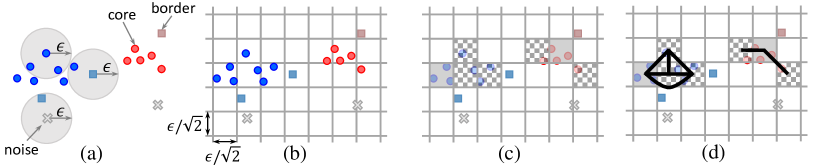
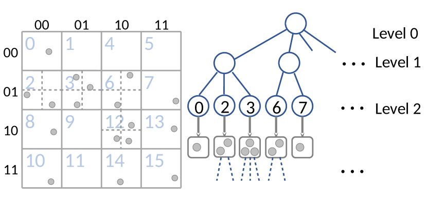
DBSCAN Definition. The DBSCAN (density-based spatial clustering of applications with noise) problem takes as input points , a distance function , and two parameters and minPts (Ester et al., 1996). A point is a core point if and only if . We denote the set of core points as . DBSCAN computes and outputs subsets of , referred to as clusters. Each point in is in exactly one cluster, and two points are in the same cluster if and only if there exists a list of points in such that . For all non-core points , belongs to cluster if for at least one point . Note that a non-core point can belong to multiple clusters. A non-core point belonging to at least one cluster is called a border point and a non-core point belonging to no clusters is called a noise point. For a given set of points and parameters and minPts, the clusters returned are unique. Similar to many previous papers on parallel DBSCAN, we focus on the Euclidean distance metric in this paper. See Figure 1(a) for an illustration of the DBSCAN problem.
Gan and Tao (Gan and Tao, 2017) define the approximate DBSCAN problem, which in addition to the DBSCAN inputs, takes a parameter . The definition is the same as DBSCAN, except for the connectivity rule among core points. In particular, core points within a distance of are still connected, but core points within a distance of may or may not be connected. Core points with distance greater than are still not connected. Due to this relaxation, multiple valid clusterings can be returned. The relaxation is what enables an asymptotically faster algorithm to be designed. A variation of this problem was described by Chen et al. (Chen et al., 2005b).
Existing algorithms as well as some of our new algorithms use subroutines for solving the bichromatic closest pair (BCP) problem, which takes as input two sets of points and , finds the closest pair of points and such that and , and returns the pair and their distance.
Computational Model. We use the work-depth model (Jaja, 1992; Cormen et al., 2009) to analyze the theoretical efficiency of parallel algorithms. The work of an algorithm is the number of operations used, similar to the time complexity in the sequential RAM model. The depth is the length of the longest sequence dependence. By Brent’s scheduling theorem (Brent, 1974), an algorithm with work and depth has overall running time , where is the number of processors available. In practice, the Cilk work-stealing scheduler (Blumofe and Leiserson, 1999) can be used to obtain an expected running time of . A parallel algorithm is work-efficient if its work asymptotically matches that of the best serial algorithm for the problem, which is important since in practice the term in the running time often dominates.
Parallel Primitives. We give an overview of the primitives used in our new parallel algorithms, and show their work and depth bounds in Table 1. We use implementations of these primitives from the Problem Based Benchmark Suite (PBBS) (Shun et al., 2012), an open-source library.
| Work | Depth | Reference | |
|---|---|---|---|
| Prefix sum, Filter | (Jaja, 1992) | ||
| Comparison sort | (Jaja, 1992; Cole, 1988) | ||
| Integer sort | (Vishkin, 2010) | ||
| Semisort | (Gu et al., 2015) | ||
| Merge | (Jaja, 1992) | ||
| Hash table | (Gil et al., 1991) | ||
| 2D Delaunay triangulation | (Reif and Sen, 1992) |
Prefix sum takes as input an array of length , and returns the array as well as the overall sum, . Prefix sum can be implemented by first adding the odd-indexed elements to the even-indexed elements in parallel, recursively computing the prefix sum for the even-indexed elements, and finally using the results on the even-indexed elements to update the odd-indexed elements in parallel. This algorithm takes work and depth (Jaja, 1992).
Filter takes an array of size and a predicate , and returns a new array containing elements for which is true, in the same order as in . We first construct an array of size with if is true and otherwise. Then we compute the prefix sum of . Finally, for each element where is true, we write it to the output array at index (i.e., ). This algorithm also takes work and depth (Jaja, 1992).
Comparison sorting sorts elements based on a comparison function. Parallel comparison sorting can be done in work and depth (Jaja, 1992; Cole, 1988). We use a cache-efficient samplesort (Blelloch et al., 2010) from PBBS which samples pivots on each level of recursion, partitions the keys based on the pivots, and recurses on each partition in parallel.
We also use integer sorting, which sorts integer keys from a polylogarithmic range in work and depth (Vishkin, 2010). The algorithm partitions the keys into sub-arrays and in parallel across all partitions, builds a histogram on each partition serially. It then uses a prefix sum on the counts of each key per partition to determine unique offsets into a global array for each partition. Finally, all partitions write their keys into unique positions in the global array in parallel.
Semisort takes as input key-value pairs, and groups pairs with the same key together, but with no guarantee on the relative ordering among pairs with different keys. Semisort also returns the number of distinct groups. We use the implementation from (Gu et al., 2015), which is available in PBBS. The algorithm first hashes the keys, and then selects a sample of the keys to predict the frequency of each key. Based on the frequency of keys in the sample, we classify them into “heavy keys” and “light keys”, and assign appropriately-sized arrays for each heavy key and each range of light keys. Finally, we insert all keys into random locations in the appropriate array and sort within the array. This algorithm takes expected work and depth with high probability.111 We say that a bound holds with high probability (w.h.p.) on an input of size if it holds with probability at least for a constant .
Merge takes two sorted arrays, and , and merges them into a single sorted array. If the sum of the lengths of the inputs is , this can be done in work and depth (Jaja, 1992). The algorithm takes equally spaced pivots and does a binary search for each pivot in . Each sub-array between pivots in has a corresponding sub-array between the binary search results in . Then it repeats the above process for each pair, except that equally spaced pivots are taken from the sub-array from and binary searches are done in the sub-array from . This creates small subproblems each of which can be solved using a serial merge, and the results are written to a unique range of indices in the final output. All subproblems can be processed in parallel.
For parallel hash tables, we can perform insertions or queries taking work and depth w.h.p. (Gil et al., 1991). We use the non-deterministic concurrent linear probing hash table from (Shun and Blelloch, 2014), which uses an atomic update to insert an element to an empty location in its probe sequence, and continues probing if the update fails.
The Delaunay triangulation on a set of points in 2D contains triangles among every triple of points , , and such that there are no other points inside the circumcircle defined by , , and (de Berg et al., 2008). Delaunay triangulation can be computed in parallel in work and depth w.h.p. (Reif and Sen, 1992). We use the randomized incremental algorithm from PBBS, which inserts points in parallel into the triangulation in rounds, such that the updates to the triangulation in each round by different points do not conflict (Blelloch et al., 2012).
3. DBSCAN Algorithm Overview
This section reviews the high-level structure of existing sequential DBSCAN algorithms (Gunawan, 2013; Gan and Tao, 2017; de Berg et al., 2017) as well as our new parallel algorithms. The high-level structure is shown in Algorithm 1, and an illustration of the key concepts are shown in Figure 1(b)-(d).
We place the points into disjoint -dimensional cells with side-length based on their coordinates (Line 2 and Figure 1(b)). The cells have the property that all points inside a cell are within a distance of from each other, and will belong to the same cluster in the end. Then on Line 3 and Figure 1(c), we mark the core points. On Line 4, we generate the clusters for core points as follows. We create a graph containing one vertex per core cell (a cell containing at least one core point), and connect two vertices if the closest pair of core points from the two cells is within a distance of . We refer to this graph as the cell graph. This step is illustrated in Figure 1(d). We then find the connected components of the cell graph to assign cluster IDs to points in core cells. On Line 5, we assign cluster IDs for border points. Finally, we return the cluster labels on Line 6.
Input: A set of points, , and minPts
Output: An array clusters of sets of cluster IDs for each point
4. 2D DBSCAN Algorithms
This section presents our parallel algorithms for implementing each line of Algorithm 1 in two dimensions. The cells can be constructed either using a grid-based method or a box-based method, which we describe in Sections 4.1 and 4.2, respectively. Section 4.3 presents our algorithm for marking core points. We present several methods for constructing the cell graph in Section 4.4. Finally, Section 4.5 describes our algorithm for clustering border points.
4.1. Grid Computation
In the grid-based method, the points are placed into disjoint cells with side-length based on their coordinates, as done in the sequential algorithms by Gunawan (Gunawan, 2013) and de Berg et al. (de Berg et al., 2017). A hash table is used to store only the non-empty cells, and a serial algorithm simply inserts each point into the cell corresponding to its coordinates.
Parallelization. The challenge in parallelization is in distributing the points to the cells in parallel while maintaining work-efficiency. While a comparison sort could be used to sort points by their cell IDs, this approach requires work and is not work-efficient. We observe that semisort (see Section 2) can be used to solve this problem work-efficiently. The key insight here is that we only need to group together points in the same cell, and do not care about the relative ordering of points within a cell or between different cells. We apply a semisort on an array of length of key-value pairs, where each key is the cell ID of a point and the value is the ID of the point. This also returns the number of distinct groups (non-empty cells).
We then create a parallel hash table of size equal to the number of non-empty cells, where each entry stores the bounding box of a cell as the key, and the number of points in the cell and a pointer to the start of its points in the semisorted array as the value. We can determine neighboring cells of a cell with arithmetic computation based on ’s bounding box, and then look up each neighboring cell in the hash table, which returns the information for that cell if it is non-empty.
4.2. Box Computation
In the box-based method, we place the points into disjoint -dimensional bounding boxes with side-length at most , which are the cells.
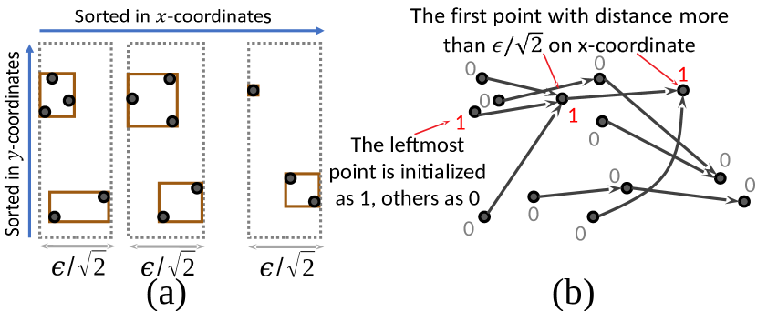
Existing sequential solutions (Gunawan, 2013; de Berg et al., 2017) first sort all points by -coordinate, then scan through the points, grouping them into strips of width and starting a new strip when a scanned point is further than distance from the beginning of the strip. It then repeats this process per strip in the -dimension to create cells of side-length at most . This step is shown in Figure 2(a). Pointers to neighboring cells are stored per cell. This is computed for all cells in each -dimensional strip by merging with each of strips , , , and , as these are the only strips that can contain cells with points within distance . For each merge, we compare the bounding boxes of the cells in increasing -coordinate, linking any two cells that may possibly have points within distance.
Parallelization. We now describe the method for assigning points to strips, which is illustrated in Figure 2(b). Let be the -coordinate of point . We create a linked list where each point is a node. The node for point stores a pointer to the node for point (we call the parent of ), where is the point with the smallest -coordinate such that . Each point can determine its parent in work and depth by binary searching the sorted list of points.
We then assign a value of to the node with the smallest -coordinate, and to all other nodes. We run a pointer jumping routine on the linked list where on each round, every node passes its value to its parent and updates its pointer to point to the parent of its parent (Jaja, 1992). The procedure terminates when no more pointers change in a round. In the end, every node with a value of will correspond to the point at the beginning of a strip, and all nodes with a value of will belong to the strip for the closest node to the left with a value of . This gives the same strips as the sequential algorithm, since all nodes marked will correspond to the closest point farther than from the point of the previously marked node. For merging to determine cells within distance , we use the parallel merging algorithm described in Section 2.
4.3. Mark Core
Illustrated in Figure 1(c), the high-level idea in marking the core points is as follows: first, if a cell contains at least minPts points then all points in the cell are core points, as it is guaranteed that all the points inside a cell will be within to any other point in the same cell; otherwise, each point computes the number of points within its -radius by checking its distance to points in all neighboring cells (defined as cells that could possibly contain points within a distance of to the current cell), and marking as a core point if the number of such points is at least minPts. For a constant dimension, only a constant number of neighboring cells need to be checked.
Parallelization. Our parallel algorithm for marking core points is shown in Algorithm 2. We create an array of length that marks which points are core points. The array is initialized to all 0’s (Line 2). We then loop through all cells in parallel (Line 3). If a cell contains at least minPts points, we mark all points in the cell as core points in parallel (Line 4–6). Otherwise, we loop through all points in the cell in parallel, and for each neighboring cell we count the number of points within a distance of to , obtained using a RangeCount(, , ) query (Lines 8–11) that reports the number of points in that are no more than distance from . The RangeCount(, , ) query can be implemented by comparing to all points in each neighboring cell in parallel, followed by a parallel prefix sum to obtain the number of points in the -radius. If the total count is at least minPts, then is marked as a core point (Lines 12–13).
4.4. Cluster Core
The next step of the algorithm is to generate the cell graph (illustrated in Figure 1(d)). We present three approaches for determining the connectivity between cells in the cell graph. After obtaining the cell graph, we run a parallel connected components algorithm to cluster the core points. For the BCP-based approach, we describe an optimization that merges the BCP computation with the connected components computation using a lock-free union-find data structure.
BCP-based Cell Graph. The problem of determining cell connectivity can be solved by computing the BCP of core points between two cells (recall the definition in Section 2), and checking whether the distance is at most .
Each cell runs a BCP computation with each of its neighboring cells to check if they should be connected in the cell graph. We execute all BCP calls in parallel, and furthermore each BCP call can be implemented naively in parallel by computing all pairwise distances in parallel, writing them into an array containing point pairs and their distances, and applying a prefix sum on the array to obtain the BCP. We apply two optimizations to speed up individual BCP calls: (1) we first filter out points further than from the other cell beforehand as done by Gan and Tao (Gan and Tao, 2017), and (2) we iterate only until finding a pair of points with distance at most , at which point we abort the rest of the BCP computation, and connect the two cells. Filtering points can be done using a parallel filter. To parallelize the early termination optimization, it is not efficient to simply parallelize across all the point comparisons as this will lead to a significant amount of wasted work. Instead, we divide the points in each cell into fixed-sized blocks, and iterate over all pairs of blocks. For each pair of blocks, we compute the distances of all pairs of points between the two blocks in parallel by writing their distances into an array. We then take the minimum distance in the array using a prefix sum, and return if the minimum is at most . This approach reduces the wasted work over the naive parallelization, while still providing ample parallelism within each pair of blocks.
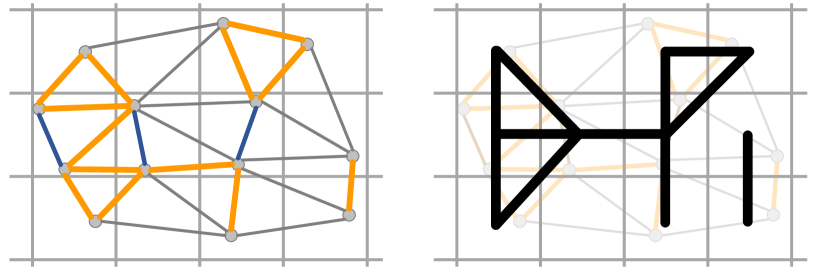
Triangulation-based Cell Graph. In two dimensions, Gunawan (Gunawan, 2013) describes a special approach using Voronoi diagrams. In particular, we can efficiently determine whether a core cell should be connected to a neighboring cell by finding the nearest core point from the neighboring cell to each of the core cell’s core points. Gan and Tao (Gan and Tao, 2017) and de Berg et al. (de Berg et al., 2017) show that a Delaunay triangulation can also be used to determine connectivity in the cell graph. In particular, if there is an edge in the Delaunay triangulation between two core cells with distance at most , then those two cells are connected. This process is illustrated in Figure 3. The proof of correctness is described in (Gan and Tao, 2017; de Berg et al., 2017).
To compute Delaunay triangulation or Voronoi diagram in parallel, Reif and Sen present a parallel algorithm for constructing Voronoi diagrams and Delaunay triangulations in two dimensions. We use the parallel Delaunay triangulation implementation from PBBS (Blelloch et al., 2012; Shun et al., 2012), as described in Section 2.
Unit-spherical emptiness checking-based (USEC) Cell Graph. Gan and Tao (Gan and Tao, 2017) (who attribute the idea to Bose et al. (Bose et al., 2007)) describe an algorithm for solving the unit-spherical emptiness checking (USEC) with line separation problem when comparing two core cells to determine whether they should be connected in the cell graph.
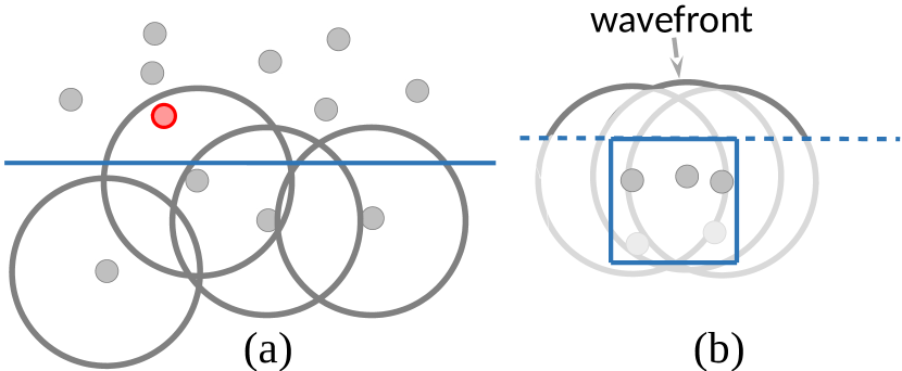
In the USEC with line separation problem, we are given a horizontal or vertical line and would like to check if any of the -radius circles of points on one side of contain any points on the other side of . The problem assumes that the points on each side of are sorted by both -coordinate and -coordinate. This is illustrated in Figure 4.
To apply the USEC with line separation problem to DBSCAN, the points in each core cell are first sorted both by -coordinate and by -coordinate (two copies are stored). For each cell, we consider its top and left boundaries as . For each , we generate the union of -radius circles centered around sorted points in the cell (sorted by -coordinate for a horizontal boundary and -coordinate for a vertical boundary) and keep the outermost arcs of the union of circles lying on the other side of , which is called the wavefront. This is illustrated in Figure 4(b). For a cell connectivity query, we choose to be one of the boundaries of the two cells that separates the two cells. Then we scan the points of one cell in sorted order and check if any of them are contained in the wavefront of the other cell.
Our algorithm assumes that all points are distinct. Without loss of generality, assume that we are generating a wavefront above a horizontal line. To generate the wavefront in parallel, we use divide-and-conquer by constructing the wavefront for the left half of the points and the right half of the points (in sorted order) recursively in parallel. Merging two wavefronts is more challenging. The wavefronts are represented as balanced binary trees supporting split and join operations (Akhremtsev and Sanders, 2016). We merge two wavefronts by taking the top part of each wavefront and joining them together. The top part of each wavefront can be obtained by checking where the left and right wavefronts intersect, and then merging them.
We prove in Section A of the Appendix that the left and right wavefronts intersect at a unique point. Denote the unique arc in the left wavefront that intersects with the right wavefront as . All the arcs to the right of in the left wavefront lie under the right wavefront, so they will not form part of the combined wavefront. On the other hand, all arcs to the left of in the left wavefront forms the left half of the combined wavefront. We find arc by doing an exponential search in the left wavefront starting from the rightmost arc. For each arc visited, we perform a binary search for in the right wavefront to find its intersection with the right wavefront. There are three possible results: (a) lies completely under the right wavefront (no intersection); (b) intersects with the right wavefront; and (c) lies completely outside the right wavefront (no intersection). If the result is (a), we continue the exponential search; if the result is (b), we terminate the search and join the two wavefronts at the intersection; and if the result is (c), arc must lie between and the previous arc visited in the exponential search, and so we continue with a binary search inside that interval to find arc . After the entire wavefront is generated, we write it out to an array by traversing the binary tree in parallel.
We can perform a cell connectivity query in parallel by creating sub-problems using pivots, similar to how parallel merge is implemented (see Section 2). Recall that we are comparing the sorted points of one cell with the wavefront of the other cell. We take equally spaced arc intersections as pivots from the wavefront, and use binary search to find where the pivot fits in the sorted point set. Every set of arcs between two pivots corresponds to a set of sorted points between two binary search results. Then we repeat the procedure on each pair by taking equally spaced pivots in the sorted point set and doing binary search of the pivot in the set of arcs (which may split an arc into multiple pieces). This gives subproblems containing a contiguous subset of the sorted points and a contiguous subset of the (possibly split) arcs of the wavefront. Each subproblem is solved using the sequential USEC with line separation algorithm of (Gan and Tao, 2017). If any of the subproblems return “yes”, then the answer to the original USEC with line separation problem is “yes”, and otherwise it is “no”.
Reducing Cell Connectivity Queries. We now present an optimization that merges the cell graph construction with the connected components computation using a parallel lock-free union-find data structure to maintain the connected components on-the-fly. This technique is used in both the BCP approach and USEC approach for cell graph construction. The pseudocode is shown in Algorithm 3. The idea is to only run a cell connectivity query between two cells if they are not yet in the same component (Line 6), which can reduce the total number of connectivity queries. For example, assume that cells , , and belong to the same component. After connecting with and with , we can avoid the connectivity check between and by checking their respective components in the union-find structure beforehand. This optimization was used by Gan and Tao (Gan and Tao, 2017) in the sequential setting, and we extend it to the parallel setting. We also only check connectivity between two cells at most once by having the cell with higher ID responsible for checking connectivity with the cell with a lower ID (Line 6).
When constructing the cell graph and checking connectivity, we use a heuristic to prioritize the cells based on the number of core points in the cells, and start from the cells with more points, as shown on Line 3. This is because cells with more points are more likely to have higher connectivity, hence connecting the nearby cells together and pruning their connectivity queries. This optimization can be less efficient in parallel, since a connectivity query could be executed before the corresponding query that would have pruned it in the sequential execution. To overcome this, we group the cells into batches, and process each batch in parallel before moving to the next batch. We refer to this new approach as bucketing, and show experimental results for it in Section 7.
4.5. Cluster Border
To assign cluster IDs for border points. We check all points not yet assigned a cluster ID, and for each point , we check all of its neighboring cells and add it to the clusters of all neighboring cells with a core point within distance to .
Parallelization. Our algorithm is shown in Algorithm 4. We loop through all cells with fewer than minPts points in parallel, and for each such cell we loop over all of its non-core points in parallel (Lines 2–3). On Lines 4–7, we check all core points in the current cell and all neighboring cells, and if any are within distance to , we add their clusters to ’s set of clusters (recall that border points can belong to multiple clusters).
5. Higher-dimensional Exact and Approximate DBSCAN
The efficient exact and approximate algorithms for higher-dimensional DBSCAN are also based on the high-level structure of Algorithm 1, and are extensions of some of the techniques for two-dimensional DBSCAN described in Section 4. They use the grid-based method for assigning points to cells (Section 4.1). Algorithms 2, 3, and 4 are used for marking core points, clustering core points, and clustering border points, respectively. However, we use two major optimizations on top of the 2D algorithms: a -d tree for finding neighboring cells and a quadtree for answering range counting queries.
5.1. Finding Neighboring Cells
The number of possible neighboring cells grows exponentially with the dimension , and so enumerating all possible neighboring cells can be inefficient in practice for higher dimensions (although still constant work in theory). Therefore, instead of implementing NeighborCells by enumerating all possible neighboring cells, we first insert all cells into a -d tree (Bentley, 1975), which enables us to perform range queries to obtain just the non-empty neighboring cells. The construction of our -d tree is done recursively, and all recursive calls for children nodes are executed in parallel. We also sort the points at each level in parallel and pass them to the appropriate child. Queries do not modify the -d tree, and can all be performed in parallel. Since a cell needs to find its neighboring cells multiple times throughout the algorithm, we cache the result on its first query to avoid repeated computation.
5.2. Range Counting
While RangeCount queries can be implemented theoretically-efficiently in DBSCAN by checking all points in the target cell, there is a large overhead for doing so in practice. In higher-dimensional DBSCAN, we construct a quadtree data structure for each cell to answer RangeCount queries. The structure of a quadtree is illustrated in Figure 5. A cell of side-length is recursively divided into sub-cells of the same size until the sub-cell becomes empty. This forms a tree where each sub-cell is a node and its children are the up to non-empty sub-cells that it divides into. Each node of the tree stores the number of points contained in its corresponding sub-cell. Queries do not modify the quadtrees and are therefore all executed in parallel. We now describe how to construct the quadtrees in parallel.
Parallel Quadtree Construction. The construction procedure recursively divides each cell into sub-cells. Each node of the tree has access to the points contained in its sub-cell in a contiguous subarray that is part of a global array (e.g., by storing a pointer to the start of its points in the global array as well as the number of points that it represents). We use an integer sort on keys from the range to sort the points in the subarray based on which of the sub-cells it belongs to. Now the points belonging to each of the child nodes are contiguous, and we can recursively construct the up to non-empty child nodes independently in parallel by passing in the appropriate subarray.
To reduce construction time, we set a threshold for the number of points in a sub-cell, below which the node becomes a leaf node. This reduces the height of the tree but makes leaf nodes larger. In addition, we avoid unnecessary tree node traversal by ensuring that each tree node has at least two non-empty children: when processing a cell, we repeatedly divide the points until they fall into at least two different sub-cells.
Range Counting in MarkCore. RangeCount queries are used in marking core points in Algorithm 2. For each cell, a quadtree containing all of its points is constructed in parallel. Then the RangeCount(, , ) query reports the number of points in cell that are no more than distance from point . Instead of naively looping through all points in , we initiate a traversal of the quadtree starting from cell , and recursively search all children whose sub-cell intersects with the -radius of . When reaching a leaf node on a query, we explicitly count the number of points contained in the -radius of the query point.
Exact DBSCAN. For higher-dimensional exact DBSCAN, one of our implementations uses RangeCount queries when computing BCPs in Algorithm 3. For each core cell, we build a quadtree on its core points in parallel. Then for each core point in each core cell , we issue a RangeCount query to each of its neighboring core cells and connect and in the cell graph if the range query returns a non-zero count of core points. Since we do not need to know the actual count, but only whether or not it is non-zero, our range query is optimized to terminate once such a result can be determined. We combine this with the optimization of reducing cell connectivity queries described in Section 4.4
Approximate DBSCAN. For approximate DBSCAN, the sequential algorithm of Gan and Tao (Gan and Tao, 2017) follows the high-level structure of Algorithm 1 using the grid-based cell structure. The only difference is in the cell graph construction, which is done using approximate RangeCount queries.
In the quadtree for approximate RangeCount, each cell of side-length is still recursively divided into sub-cells of the same size, but until either the sub-cell becomes empty or has side-length at most . The tree has maximum depth . We use a modified version of our parallel quadtree construction method to parallelize approximate DBSCAN.
An approximate RangeCount(, , , ) query takes as input a point , and returns an integer that is between the number of points in the -radius and the number of points in the -radius of that are in , (when using approximate RangeCount, all relevant methods takes an additional parameter ). If the answer is non-zero, then the core cell containing is connected to core cell . Our query implementation starts a traversal of the quadtree from , and recursively searches all children whose sub-cell intersects with the -radius of . As done in exact DBSCAN, our query is optimized to terminate once a zero count or a non-zero count can be determined. Once either a leaf node is reached or a node’s sub-cell is completely contained in the -radius of , the search on that path terminates. Queries do not modify the quadtree and can all be executed in parallel.
6. Analysis
This section analyzes the theoretical complexity of our algorithms, showing that they are work-efficient and have polylogarithmic depth.
6.1. 2D Algorithms
Grid Computation. In our parallel algorithm presented in Section 4.1, creating key-value pairs can be done in work and depth in a data-parallel fashion. Semisorting takes expected work and depth w.h.p. Constructing the hash table and inserting non-empty cells into it takes work and depth w.h.p. The overall cost of the parallel grid computation is therefore work in expectation and depth w.h.p.
Box Computation. The serial algorithm (Gunawan, 2013; de Berg et al., 2017) uses work, including sorting, scanning the points to assign them to strips and cells, and merging strips. However, the span is since in the worst case there can be strips.
Parallel comparison sorting takes work and depth. Therefore, sorting the points by -coordinate, and each strip by -coordinate can be done in work and depth overall. Parent finding using binary search for all points takes work and depth. For pointer jumping, the longest path in the linked list halves on each round, and so the algorithm terminates after rounds. We do work per round, leading to an overall work of . The depth is per round, for a total of overall. We repeat this process for the points in each strip, but in the -direction, and the work and depth bounds are the same. For assigning pointers to neighboring cells for each cell, we use a parallel merging algorithm, which takes work and depth. The pointers are stored in an array, accessible in constant work and depth.
MarkCore. For cells with at least minPts points, we spend work overall marking their points as core points (Lines 4–6 of Algorithm 2). All cells are processed in parallel, and all points can be marked in parallel, giving depth.
For all cells with fewer than minPts points, each point only needs to execute a range count query on a constant number of neighboring cells (Gunawan, 2013; Gan and Tao, 2017). RangeCount(, , ) compares to all points in neighboring cell in parallel. Across all queries, each cell will only be checked by many points, and so the overall work for range counting is . Therefore, Lines 8–13 of Algorithm 2 takes work. All points are processed in parallel, and there are a constant number of RangeCount calls per point, each of which takes depth for a parallel prefix sum to obtain the number of points in the -radius. Therefore, the depth for range counting is .
The work for looking up the neighbor cells is and depth is w.h.p. using the parallel hash table that stores the non-empty cells. Therefore, parallel MarkCore takes work and depth w.h.p.
Cell Graph Construction. Reif and Sen present a parallel algorithm for constructing Voronoi diagrams and Delaunay triangulations in two dimensions in work and depth w.h.p. (Reif and Sen, 1992). For the Voronoi diagram approach, each nearest neighbor query can be answered in work, which is used to check whether two cells should be connected and can be applied in parallel. Each cell will only execute a constant number of queries, and so the overall complexity is work and depth w.h.p. For the Delaunay triangulation approach, we can simply apply a parallel filter over all of the edges in the triangulation, keeping the edges between different cells with distance at most . The cost of the filter is dominated by the cost of constructing the Delaunay triangulation.
For the USEC with line separation method, the sorted order of points in each dimension for each cell can be generated in work and depth overall. To generate a wavefront on points, the exponential search has steps per level, and each step involves a binary search which takes work and depth. Therefore, the the work and depth for the searches is per level. Splitting and joining the binary trees to generate the new wavefront on each level takes work and depth (Akhremtsev and Sanders, 2016). Thus, for the work, we obtain the recurrence , which solves to . Since we can solve the recursive subproblems in parallel, for the depth, we obtain the recurrence , which solves to .
Checking whether the sorted set of points from one cell intersects with a wavefront from another cell can be done using an algorithm similar to parallel merging, as described in Section 4.4. In particular, for a wavefront of size and sorted point set of size , we pick equally spaced pivots from the wavefront, and use binary search to split the sorted point set into subsets of size where . The binary searches take a total of work and depth. Then, for the ’th pair forming a subproblem, we pick equally spaced pivots from the ’th subset of points and perform a binary search into the ’th subset of arcs of the wavefront to create more subproblems. This takes a total of work and depth. The subset of points and subset of arcs for each subproblem are now all guaranteed to be of size . In parallel across all subproblems, we run the serial USEC with line separation algorithm of (Gan and Tao, 2017), which takes linear work in the input size. Therefore, the work for this particular instance of USEC with line separation is and the depth is . All cell connectivity queries can be performed in parallel, and so the total work is and and depth is . Since the sequential algorithms for wavefront generation and determining cell connectivity take linear work, our algorithm is work-efficient. After generating each wavefront, we write it out to an array by traversing the binary tree in parallel, which takes linear work and logarithmic depth (Akhremtsev and Sanders, 2016). Including the preprocessing step of sorting, our parallel USEC with line separation problem for determining the connectivity of core cells takes work and depth.
Connected Components. After the cell graph that contains points and edges are constructed, we run connected components on the cell graph. This step can be done in parallel in work and depth w.h.p. using parallel connectivity algorithms (Gazit, 1991; Halperin and Zwick, 1994; Cole et al., 1996; Halperin and Zwick, 2001; Pettie and Ramachandran, 2002).
ClusterBorder. Using a similar analysis as done for marking core points, it can be shown that assigning cluster IDs to border points takes work sequentially (Gunawan, 2013; de Berg et al., 2017). In parallel, since there are a constant number of neighboring cells for each non-core point, and all points in neighboring cells as well as all non-core points are checked in parallel, the depth is for the distance comparisons. Looking up the neighboring cells can be done in work and depth w.h.p. using our parallel hash table. Adding cluster IDs to border point’s set of clusters, while removing duplicates at the same time, can be done using parallel hashing in linear work and depth w.h.p. The work is since we do not introduce any asymptotic work overhead compared to the sequential algorithm.
Overall, we have the following theorem.
Theorem 6.1.
For a constant value of minPts, 2D Euclidean DBSCAN can be computed in work and depth w.h.p.
6.2. Higher-dimensional Algorithm
For dimensions, the BCP problem can be solved either using brute-force checking, which takes quadratic work, or using more theoretically-efficient algorithms that take sub-quadratic work (Agarwal et al., 1991; Chazelle, 1985; Clarkson, 1988). This leads to a DBSCAN algorithm that takes expected work for and expected work for where is any constant (Gan and Tao, 2017). The theoretically-efficient BCP algorithms seem too complicated to be practical (we are not aware of any implementations of these algorithms), and the actual implementation of (Gan and Tao, 2017) does not use them. However, we believe that it is still theoretically interesting to design a sub-quadratic work parallel BCP algorithm to use in DBSCAN, which is the focus of this section.
The sub-quadratic work BCP algorithms are based on constructing Delaunay triangulations (DT) in dimensions, which can be used for nearest neighbor search. However, we cannot afford to construct a DT on all the points, since a -dimensional DT contains up to simplices, which is at least quadratic in the worst-case for .
The idea in the algorithm by Agarwal et al. (Agarwal et al., 1991) is to construct multiple DTs, each for a subset of the points, and a nearest neighbor query then takes the closest neighbor among queries to all of the DTs. The data structure for nearest neighbor queries used by Aggarwal et al. is based on the RPO (Randomized Post Office) tree by Clarkson (Clarkson, 1988). The RPO tree contains levels where each node in the RPO tree corresponds to the DT of a random subset of the points. Parallel DT for a constant dimension can be computed work-efficiently in expectation and in depth w.h.p. (Blelloch et al., 2018). The children of each node can be determined by traversing the history graph of the DT, which takes work and depth. The RPO tree is constructed recursively for levels, and so the overall depth is w.h.p. A query traverses down a path in the RPO tree, querying each DT along the path, which takes work and depth overall. Using this data structure to solve BCP gives a DBSCAN algorithm with expected work and depth w.h.p. For , an improved data structure by Agarwal et al. (Agarwal et al., 1990) can be used to improve the expected work to . The data structure is also based on DT, and so similar to before, we can parallelize the DT construction and obtain the same depth bound.
The overall bounds are summarized in the following theorem.
Theorem 6.2.
For a constant value of minPts, Euclidean DBSCAN can be solved in expected work for and expected work for any constant for , and polylogarithmic depth with high probability.
6.3. Approximate Algorithm
The algorithms for grid construction, marking core points, connected components, and clustering border points are the same as the exact algorithms, and so we only analyze approximate cell graph construction in the approximate algorithm based on the quadtree introduced in Section 5.2. The quadtree has levels and can be constructed in work sequentially for a cell with points. A hash table is used to map non-empty cells to their quadtrees, which takes work w.h.p. to construct. Using a fact from (Arya and Mount, 2000), Gan and Tao show that the number of nodes visited by a query is . Therefore, for constant and , all of the quadtrees can be constructed in a total of work w.h.p., and queries can be answered in expected work.
All of the quadtrees can be constructed in parallel. To parallelize the construction of a quadtree for a cell with points, we sort the points on each level in work and depth using parallel integer sorting (Vishkin, 2010), since the keys are integers in a constant range. In total, this gives work and depth per quadtree. We use a parallel hash table to map non-empty cells to their quadtrees, which takes work and depth w.h.p. to construct. To construct the cell graph, all core points issue a constant number of queries to neighboring cells in parallel. The hash table queries can be done in work and depth w.h.p. and thus cell graph construction has the same complexity. This gives the following theorem.
Theorem 6.3.
For constant values of minPts and , our approximate Euclidean DBSCAN algorithm takes work and depth with high probability.
7. Experiments
This section presents experiments comparing our exact and approximate algorithms as well as existing algorithms.
Datasets. We use the synthetic seed spreader (SS) datasets produced by Gan and Tao’s generator (Gan and Tao, 2017). The generator produces points generated by a random walk in a local neighborhood, but jumping to a random location with some probability. SS-simden and SS-varden refer to the datasets with similar-density and variable-density clusters, respectively. We also use a synthetic dataset called UniformFill that contains points distributed uniformly at random inside a bounding hypergrid with side length , where is the total number of points. The points have double-precision floating point values, but we scaled them to integers when testing Gan and Tao’s implementation, which requires integer coordinates. We generated the synthetic datasets with 10 million points (unless specified otherwise) for dimensions .
In addition, we use the following real-world datasets, which contain points with double-precision floating point values.
-
(1)
Household (Dua and Graff, 2017) is a 7-dimensional dataset with points excluding the date-time information.
-
(2)
GeoLife (Zheng et al., 2008) is a 3-dimensional dataset with points. This dataset contains user location data (longitude, latitude, altitude), and its distribution is extremely skewed.
-
(3)
Cosmo50 (Kwon et al., 2010) is a 3-dimensional dataset with points. We extracted the , , and coordinate information to construct the 3-dimensional dataset.
-
(4)
OpenStreetMap (Haklay and Weber, 2008) is a 2-dimensional dataset with points, containing GPS location data.
-
(5)
TeraClickLog (CriteoLabs, 2013) is a 13-dimensional dataset with
points containing feature values and click feedback of online advertisements. As far as we know, TeraClickLog is the largest dataset used in the literature for exact DBSCAN.
We performed a search on and minPts for the synthetic datasets and chose the default parameters to be those that output a correct clustering. For the SS datasets, the default parameters that we use are similar to those found by Gan and Tao (Gan and Tao, 2017). For ease of comparison, the default parameters for Household are the same as Gan and Tao (Gan and Tao, 2017) and the default parameters for GeoLife, Cosmo50, OpenStreetMap, and TeraClickLog are same as RP-DBSCAN (Song and Lee, 2018). For approximate DBSCAN, we set , unless specified otherwise.
Testing Environment. We perform all of our experiments on Amazon EC2 machines. We use a c5.18xlarge machine for testing of all datasets other than Cosmo50, OpenStreetMap, and TeraClickLog. The c5.18xlarge machine has 2 Intel Xeon Platinum 8124M (3.00GHz) CPUs for a total for a total of 36 two-way hyper-threaded cores, and 144 GB of RAM. We use a r5.24xlarge machine for the three larger datasets just mentioned. The r5.24xlarge machine has 2 Intel Xeon Platinum 8175M (2.50 GHz) CPUs for a total of 48 two-way hyper-threaded cores, and 768 GB of RAM. By default, we use all of the cores with hyper-threading on each machine. We compile our programs with the g++ compiler (version 7.4) with the -O3 flag, and use Cilk Plus for parallelism (Leiserson, 2010).
7.1. Algorithms Tested
We implement the different methods for marking core points and BCP computation in exact and approximate DBSCAN for , and present results for the fastest versions, which are described below.
- •
- •
-
•
our-approx: This approximate implementation implements the RangeCount query in marking core points by scanning through all points in the neighboring cell in parallel, and uses the quadtree for approximate RangeCount queries in cell graph construction described in Section 5.2.
-
•
our-approx-qt: This approximate implementation is the same as our-approx except that it uses the RangeCount query supported by the quadtree described in Section 5.2 for marking core points.
We append the -bucketing suffix to the names of these implementations when using the bucketing optimization described in Section 4.4.
For , we have six implementations that differ in whether they use the grid or the box method to construct cells and whether they use BCP, Delaunay triangulation, or USEC with line separation to construct the cell graph. We refer to these as our-2d-grid-bcp, our-2d-grid-usec, our-2d-grid-delaunay, our-2d-box-bcp, our-2d-box-usec, and our-2d-box-delaunay.
We note that our exact algorithms return the same answer as the standard DBSCAN definition, and our approximate algorithms return answers that satisfy Gan and Tao’s approximate DBSCAN definition (see Section 2).
We compare with the following implementations:
-
•
Gan&Tao-v2 (Gan and Tao, 2017) is the state-of-the-art serial implementation for both exact and approximate DBSCAN. Gan&Tao-v2 only accepts integer values between and , and so when running their code we scaled the datasets up into this integer range and scaled up the value accordingly to achieve a consistent clustering output with other methods.
-
•
pdsdbscan (Patwary et al., 2013) is the implementation of the parallel disjoint-set exact DBSCAN by Patwary et al. compiled with OpenMP.
-
•
hpdbscan (Götz et al., 2015) is the implementation of parallel exact DBSCAN by Gotz et al. compiled with OpenMP. We modified the source code to remove the file output code.
-
•
rpdbscan (Song and Lee, 2018) is the state-of-the-art distributed implementation for DBSCAN using Apache Spark. We note that their variant does not return the same result as DBSCAN. We tested rpdbscan on the same machine that we used, and also report the timings in (Song and Lee, 2018), which were obtained using at least as many cores as our largest machine.
7.2. Experiments for
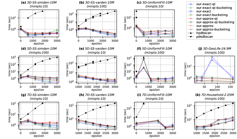
We first evaluate the performance of the different algorithms for . In the following plots, data points that did not finish within an hour are not shown.
Influence of on Parallel Running Time. In this experiment, we fix the default value of minPts corresponding to the correct clustering, and vary within a range centered around the default value. Figure 6 shows the parallel running time vs. for the different implementations. In general, both pdsdbscan and hpdbscan becomes slower with increasing . This is because they use pointwise range queries, which get more expensive with larger . Our methods tend to improve with increasing because there are fewer cells leading to a smaller cell graph, which speeds up computations on the graph. Our implementations significantly outperform pdsdbscan and hpdbscan on all of the data points.
We observe a spike in plot Figure 6(f) when . The implementations that mark core points by scanning through all points in neighboring cells spend a significant amount of time in that phase; in comparison, the quadtree versions perform better because of their more optimized range counting. There is also a spike in Figure 6(j) when . Our exact implementation spends a significant amount of time in cell graph construction. This is because the GeoLife dataset is heavily skewed, certain cells could contain significantly more points. When many cell connectivity queries involve these cells, the quadratic nature using the BCP approach in our-exact makes the cost of queries expensive. On the contrary, methods using the quadtree for cell graph construction (our-exact-qt, our-approx-qt, and our-approx) tend to have consistent performance across the values. For the spike in Figure 6(j), it is interesting to see that the bucketing implementations, our-exact-qt-bucketing and our-exact-bucketing, are significantly faster than our-exact-qt and our-exact because many of the expensive connectivity queries are pruned.
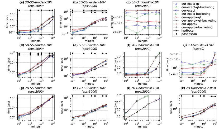
Influence of minPts on Parallel Running Time. In this experiment, we fix the default value of for a dataset and vary minPts over a range from to . Figure 7 shows that our implementations have an increasing trend in running time as minPts increases in most cases. This is consistent with our analysis in Section 6.1 that the overall work for marking core points is . In contrast, minPts does not have much impact on the performance of hpdbscan and pdsdbscan because their range queries, which dominate the total running times, do not depend on minPts. Our implementations outperform hpdbscan and pdsdbscan for almost all values of minPts. Figures 7(d) and 7(g) suggests that hpdbscan can surpass our performance for certain datasets when . However, as suggested by Schubert et al. (Schubert et al., 2017), the minPts value used in practice is usually much smaller, and based on our observation, a minPts value of at most 100 usually gives the correct clusters.
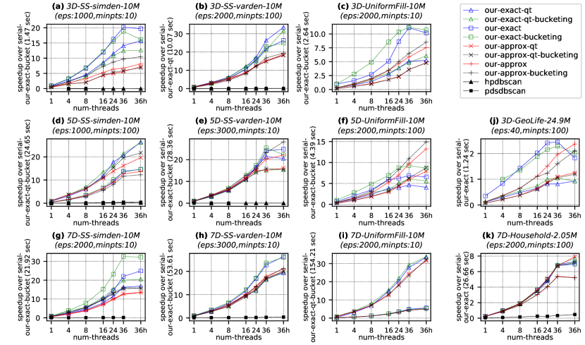
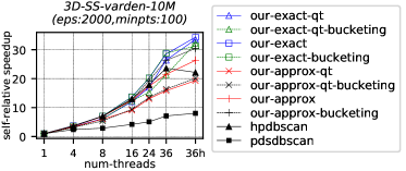
Parallel Speedup. To the best of our knowledge, Gan&Tao-v2 is the fastest existing serial implementation both for exact and approximate DBSCAN. However, we find that across all of our datasets, our serial implementations are faster than theirs by an average of 5.18x and 1.52x for exact DBSCAN and approximate DBSCAN, respectively. In Figure 8, we compare the speedup of the parallel implementations under different thread counts over the best serial baselines for each dataset and choice of parameters. We also show the self-relative speedups for one dataset in Figure 9 and note that the trends are similar on other datasets. For these experiments, we use parameters that generate the correct clusters. Our implementations obtain very good speedups on most datasets, achieving speedups of 5–33x (16x on average) over the best serial baselines. Additionally, the self-relative speedups of our exact and approximate methods are 2–89x (24x on average) and 14-44x (24x on average), respectively. Although hpdbscan and pdsdbscan achieve good self-relative speedup (22–31x and 7–20x, respectively), they fail to outperform the serial implementation on most of the datasets. Compared to hpdbscan and pdsdbscan, we are faster by up to orders of magnitude (16–6102x).
Our speedup on the GeoLife dataset (Figure 8(j)) is low due to the high skewness of cell connectivity queries caused by the skewed point distribution, however the parallel running time is reasonable (less than 1 second). In contrast, hpdbscan and pdsdbscan did not terminate within an hour.
The bucketing heuristic achieved the best parallel performance for several of the datasets (Figures 6(f), (g), and (j); Figures 7(c) and (j); and Figures 8(c), (f), (g), and (j)). In general, the bucketing heuristic greatly reduces the number of connectivity queries during cell graph construction, but in some cases it can reduce parallelism and/or increase overhead due to sorting. We also observe a similar trend on all methods where bucketing is applied.
We also implemented our own parallel baseline based on the original DBSCAN algorithm (Ester et al., 1996). We use a parallel -d tree, and all points perform queries in parallel to find all neighbors in their -radius to check if they should be a core point. However, the baseline was over 10x slower than our fastest parallel implementation for datasets with the correct parameters, and hence we do not show it in the plots.
| GeoLife | Cosmo50 | OpenStreetMap | TeraClickLog | |||||||||||||
| 20 | 40 | 80 | 160 | 0.01 | 0.02 | 0.04 | 0.08 | 0.01 | 0.02 | 0.04 | 0.08 | 1500 | 3000 | 6000 | 12000 | |
| our-exact | 0.541 | 0.617 | 0.535 | 0.482 | 41.8 | 5.51 | 4.69 | 3.03 | 41.4 | 43.2 | 40 | 44.5 | 26.8 | 26.9 | 27.0 | 27.6 |
| rpdbscan (our machine) | 29.13 | 27.92 | 32.04 | 27.81 | 3750 | 562.0 | 576.9 | 672.6 | – | – | – | – | – | – | – | – |
| rpdbscan ((Song and Lee, 2018)) | 36 | 33 | 28 | 27 | 960 | 504 | 438 | 432 | 3000 | 1720 | 1200 | 840 | 15480 | 7200 | 3540 | 1680 |
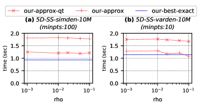
Influence of on Parallel Running Time. Figure 10 shows the effect of varying for our two approximate DBSCAN implementations. We also show our best exact method as a baseline. We only show plots for two datasets as the trend was similar in other datasets. We observe a small decrease in running time as increases, but find that the approximate methods are still mostly slower than the best exact method. On average, for the parameters corresponding to correct clustering, we find that our best exact method is 1.24x and 1.53x faster than our best approximate method when running in parallel and serially, respectively; this can also be seen in Figure 8. Schubert et al. (Schubert et al., 2017) also found exact DBSCAN to be faster than approximate DBSCAN for appropriately-chosen parameters, which is consistent with our observation.
Large-scale Datasets. In Table 2, we show the running times of our-exact on large-scale datasets. We compare with the reported numbers for the state-of-the-art distributed implementation rpdbscan, which use 48 cores distributed across 12 machines (Song and Lee, 2018), as well as numbers for rpdbscan on our machines. The purpose of this experiment is to show that we are able to efficiently process large datasets using just a multicore machine. GeoLife was run on the 36 core machine whereas others were run on the 48 core machine due to their larger memory footprint. We see that our-exact achieves a 18–577x speedup over rpdbscan using the same or a fewer number of cores. We believe that this speedup is due to lower communication costs in shared-memory as well as a better algorithm. Even though TeraClickLog is significantly larger than the other datasets, our running times are not proportionally larger. This is because for the parameters chosen by (Song and Lee, 2018), all points fall into one cell. Therefore, in our implementation all points are core points and are trivially placed into the only cluster. In contrast, rpdbscan incurs communication costs in partitioning the points across machines and merging the clusters from different machines together.
7.3. Experiments for
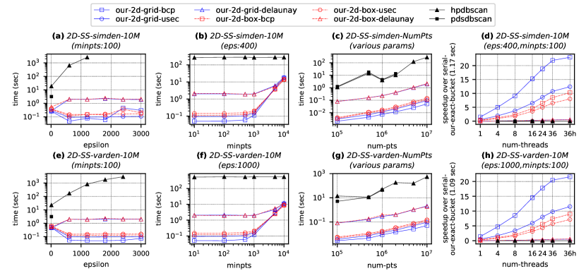
In Figure 11, we show the performance of our six 2D algorithms as well as hpdbscan and pdsdbscan on the synthetic datasets. We show the running time while varying , minPts, number of points, or number of threads. We first note that all of our implementations are significantly faster than hpdbscan and pdsdbscan. In general, we found the grid-based implementations to be faster than the box-based implementations due to the higher cell construction time of the boxed-based implementations. We also found the Delaunay triangulation-based implementations to be significantly slower than the BCP and USEC-based methods due to the high overhead of computing the Delaunay triangulation. The fastest implementation overall was our-2d-grid-bcp.
8. Related Work
Xu et al. (Xu et al., 1999) provide the first parallel exact DBSCAN algorithm, called PDBSCAN, based on a distributed -tree. Arlia and Coppola (Arlia and Coppola, 2001) present a parallel DBSCAN implementation that replicates a sequential -tree across machines to process points in parallel. Coppola and Vanneschi (Coppola and Vanneschi, 2002) design a parallel algorithm using a queue to store core points, where each core point is processed one at a time but their neighbors are checked in parallel to see whether they should be placed at the end of the queue. Januzaj et al. (Januzaj et al., 2004a, b) design an approximate DBSCAN algorithm based on determining representative points on different local processors, and then running a sequential DBSCAN on the representatives. Brecheisen et al. (Brecheisen et al., 2006) parallelize a version of DBSCAN optimized for complex distance functions (Brecheisen et al., 2004).
Patwary et al. (Patwary et al., 2012) present PDSDBSCAN, a multicore and distributed algorithm for DBSCAN using a union-find data structure for connecting points. Their union-find data structure is lock-based whereas ours is lock-free. Patwary et al. (Patwary et al., 2014; Patwary et al., 2015) also present distributed DBSCAN algorithms that are approximate but more scalable than PDSDBSCAN. Hu et al. (Hu et al., 2017) design PS-DBSCAN, an implementation of DBSCAN using a parameter server framework. Gotz et al. (Götz et al., 2015) present HPDBSCAN, an algorithm for both shared-memory and distributed-memory based on partitioning the data among processors, running DBSCAN locally on each partition, and then merging the clusters together. Very recently, Sarma et al. (Sarma et al., 2019) present a distributed algorithm, DBSCAN, and report a running time of 41 minutes for clustering one billion 3-dimensional points using a cluster of 32 nodes. Our running times on the larger 13-dimensional TeraClickLog dataset are significantly faster (under 30 seconds on 48 cores).
Exact and approximate distributed DBSCAN algorithms have been designed using MapReduce (Xiang Fu et al., 2011; Dai and Lin, 2012; He et al., 2014; Fu et al., 2014; Kim et al., 2014; Yu et al., 2015; Araujo Neto et al., 2015; Hu et al., 2018) and Spark (Cordova and Moh, 2015; Han et al., 2016; Luo et al., 2016; Huang et al., 2017; Song and Lee, 2018; Lulli et al., 2016). RP-DBSCAN (Song and Lee, 2018), an approximate DBSCAN algorithm, has been shown to be the state-of-the-art for MapReduce and Spark. GPU implementations of DBSCAN have also been designed (Böhm et al., 2009; Andrade et al., 2013; Welton et al., 2013; Chen and Chen, 2015).
In addition to parallel solutions, there have been optimizations proposed to speed up sequential DBSCAN (Brecheisen et al., 2004; Kryszkiewicz and Lasek, 2010; Mahesh Kumar and Rama Mohan Reddy, 2016). DBSCAN has also been generalized to other definitions of neighborhoods (Sander et al., 1998). Furthermore, there have been variants of DBSCAN proposed in the literature, which do not return the same result as the standard DBSCAN. IDBSCAN (Borah and Bhattacharyya, 2004), FDBSCAN (Liu, 2006), GF-DBSCAN (Tsai and Wu, 2009), I-DBSCAN (Viswanath and Pinkesh, 2006), GNDBSCAN (Huang and Bian, 2009), Rough-DBSCAN (Viswanath and Babu, 2009), and DBSCAN++ (Jang and Jiang, 2019) use sampling to reduce the number of range queries needed. El-Sonbaty et al. (El-Sonbaty et al., 2004) presents a variation that partitions the dataset, runs DBSCAN within each partition, and merges together dense regions. GriDBSCAN (Mahran and Mahar, 2008) uses a similar idea with an improved scheme for partitioning and merging. Other partitioning based algorithms include PACA-DBSCAN (Jiang et al., 2011), APSCAN (Chen et al., 2011), and AA-DBSCAN (Kim et al., 2019). DBSCAN∗ and H-DBSCAN∗ are variants of DBSCAN where only core points are included in clusters (Campello et al., 2015). Other variants use approximate neighbor queries to speed up DBSCAN (Wu et al., 2007; He et al., 2017).
OPTICS (Ankerst et al., 1999), SUBCLU (Kailing et al., 2004), and GRIDBSCAN (Uncu et al., 2006), are hierarchical versions of DBSCAN that compute DBSCAN clusters on different parameters, enabling clusters of different densities to more easily be found. POPTICS (Patwary et al., 2013) is a parallel version of OPTICS based on concurrent union-find.
9. Conclusion
We have presented new parallel algorithms for exact and approximate Euclidean DBSCAN that are both theoretically-efficient and practical. Our algorithms are work-efficient and have polylogarithmic depth, making them highly parallel. Our experiments demonstrate that our solutions achieve excellent parallel speedup and significantly outperform existing parallel DBSCAN solutions. Future work includes designing theoretically-efficient and practical parallel algorithms for variants of DBSCAN and hierarchical versions of DBSCAN.
Acknowledgements
This research was supported by DOE Early Career Award #DE-SC0018947, NSF CAREER Award #CCF-1845763, Google Faculty Research Award, DARPA SDH Award #HR0011-18-3-0007, and Applications Driving Architectures (ADA) Research Center, a JUMP Center co-sponsored by SRC and DARPA.
References
- (1)
- Agarwal et al. (1990) Pankaj K. Agarwal, Herbert Edelsbrunner, Otfried Schwarzkopf, and Emo Welzl. 1990. Euclidean Minimum Spanning Trees and Bichromatic Closest Pairs. In Annual Symposium on Computational Geometry. 203–210.
- Agarwal et al. (1991) Pankaj K. Agarwal, Herbert Edelsbrunner, Otfried Schwarzkopf, and Emo Welzl. 1991. Euclidean minimum spanning trees and bichromatic closest pairs. Discrete & Computational Geometry 6, 3 (01 Sep 1991), 407–422.
- Akhremtsev and Sanders (2016) Y. Akhremtsev and P. Sanders. 2016. Fast Parallel Operations on Search Trees. In IEEE International Conference on High Performance Computing (HiPC). 291–300.
- Andrade et al. (2013) Guilherme Andrade, Gabriel Ramos, Daniel Madeira, Rafael Sachetto, Renato Ferreira, and Leonardo Rocha. 2013. G-DBSCAN: A GPU Accelerated Algorithm for Density-based Clustering. Procedia Computer Science 18 (2013), 369 – 378.
- Ankerst et al. (1999) Mihael Ankerst, Markus M. Breunig, Hans-Peter Kriegel, and Jörg Sander. 1999. OPTICS: Ordering Points to Identify the Clustering Structure. In ACM International Conference on Management of Data (SIGMOD). 49–60.
- Araujo Neto et al. (2015) Antonio Cavalcante Araujo Neto, Ticiana Linhares Coelho da Silva, Victor Aguiar Evangelista de Farias, José Antonio F. Macêdo, and Javam de Castro Machado. 2015. G2P: A Partitioning Approach for Processing DBSCAN with MapReduce. In Web and Wireless Geographical Information Systems. 191–202.
- Arlia and Coppola (2001) Domenica Arlia and Massimo Coppola. 2001. Experiments in Parallel Clustering with DBSCAN. In European Conference on Parallel Processing (Euro-Par). 326–331.
- Arya and Mount (2000) Sunil Arya and David M. Mount. 2000. Approximate range searching. Computational Geometry 17, 3 (2000), 135 – 152.
- Bentley (1975) Jon Louis Bentley. 1975. Multidimensional Binary Search Trees Used for Associative Searching. Commun. ACM 18, 9 (Sept. 1975), 509–517.
- Blelloch et al. (2012) Guy E. Blelloch, Jeremy T. Fineman, Phillip B. Gibbons, and Julian Shun. 2012. Internally Deterministic Parallel Algorithms Can Be Fast. In ACM SIGPLAN Symposium on Proceedings of Principles and Practice of Parallel Programming (PPoPP). 181–192.
- Blelloch et al. (2010) Guy E. Blelloch, Phillip B. Gibbons, and Harsha Vardhan Simhadri. 2010. Low-Depth Cache Oblivious Algorithms. In ACM Symposium on Parallelism in Algorithms and Architectures (SPAA). 189–199.
- Blelloch et al. (2018) Guy E. Blelloch, Yan Gu, Julian Shun, and Yihan Sun. 2018. Parallelism in Randomized Incremental Algorithms. CoRR abs/1810.05303 (2018). arXiv:1810.05303
- Blumofe and Leiserson (1999) Robert D. Blumofe and Charles E. Leiserson. 1999. Scheduling Multithreaded Computations by Work Stealing. J. ACM 46, 5 (Sept. 1999), 720–748.
- Böhm et al. (2009) Christian Böhm, Robert Noll, Claudia Plant, and Bianca Wackersreuther. 2009. Density-based Clustering Using Graphics Processors. In ACM Conference on Information and Knowledge Management. 661–670.
- Borah and Bhattacharyya (2004) B. Borah and D. K. Bhattacharyya. 2004. An improved sampling-based DBSCAN for large spatial databases. In International Conference on Intelligent Sensing and Information Processing. 92–96.
- Bose et al. (2007) Prosenjit Bose, Anil Maheshwari, Pat Morin, Jason Morrison, Michiel Smid, and Jan Vahrenhold. 2007. Space-efficient geometric divide-and-conquer algorithms. Computational Geometry 37, 3 (2007), 209 – 227.
- Brecheisen et al. (2004) S. Brecheisen, H. Kriegel, and M. Pfeifle. 2004. Efficient density-based clustering of complex objects. In IEEE International Conference on Data Mining (ICDM). 43–50.
- Brecheisen et al. (2006) Stefan Brecheisen, Hans-Peter Kriegel, and Martin Pfeifle. 2006. Parallel Density-Based Clustering of Complex Objects. In Advances in Knowledge Discovery and Data Mining (PAKDD). 179–188.
- Brent (1974) Richard P. Brent. 1974. The Parallel Evaluation of General Arithmetic Expressions. J. ACM 21, 2 (April 1974), 201–206.
- Campello et al. (2015) Ricardo Campello, Davoud Moulavi, Arthur Zimek, and Jörg Sander. 2015. Hierarchical Density Estimates for Data Clustering, Visualization, and Outlier Detection. ACM Trans. Knowl. Discov. Data 10, 1, Article 5 (July 2015), 5:1–5:51 pages.
- Chazelle (1985) Bernard Chazelle. 1985. How to search in history. Information and control 64, 1-3 (1985), 77–99.
- Chen and Chen (2015) Chun-Chieh Chen and Ming-Syan Chen. 2015. HiClus: Highly Scalable Density-based Clustering with Heterogeneous Cloud. Procedia Computer Science 53 (2015), 149 – 157.
- Chen et al. (2005a) Danny Z. Chen, Michiel Smid, and Bin Xu. 2005a. Geometric Algorithms for Density-Based Data Clustering. International Journal of Computational Geometry & Applications 15, 03 (2005), 239–260.
- Chen et al. (2005b) Danny Z Chen, Michiel Smid, and Bin Xu. 2005b. Geometric algorithms for density-based data clustering. International Journal of Computational Geometry & Applications 15, 03 (2005), 239–260.
- Chen et al. (2011) Xiaoming Chen, Wanquan Liu, Huining Qiu, and Jianhuang Lai. 2011. APSCAN: A parameter free algorithm for clustering. Pattern Recognition Letters 32, 7 (2011), 973 – 986.
- Clarkson (1988) Kenneth L Clarkson. 1988. A randomized algorithm for closest-point queries. SIAM J. Comput. 17, 4 (1988), 830–847.
- Cole (1988) Richard Cole. 1988. Parallel Merge Sort. SIAM J. Comput. 17, 4 (Aug. 1988), 770–785.
- Cole et al. (1996) Richard Cole, Philip N. Klein, and Robert E. Tarjan. 1996. Finding Minimum Spanning Forests in Logarithmic Time and Linear Work Using Random Sampling. In ACM Symposium on Parallel Algorithms and Architectures (SPAA). 243–250.
- Coppola and Vanneschi (2002) Massimo Coppola and Marco Vanneschi. 2002. High-performance Data Mining with Skeleton-based Structured Parallel Programming. Parallel Comput. 28, 5 (May 2002), 793–813.
- Cordova and Moh (2015) I. Cordova and T. Moh. 2015. DBSCAN on Resilient Distributed Datasets. In International Conference on High Performance Computing Simulation (HPCS). 531–540.
- Cormen et al. (2009) Thomas H. Cormen, Charles E. Leiserson, Ronald L. Rivest, and Clifford Stein. 2009. Introduction to Algorithms (3. ed.). MIT Press.
- CriteoLabs (2013) CriteoLabs. 2013. Terabyte Click Logs. http://labs.criteo.com/downloads/download-terabyte-click-logs/
- Dai and Lin (2012) B. Dai and I. Lin. 2012. Efficient Map/Reduce-Based DBSCAN Algorithm with Optimized Data Partition. In IEEE International Conference on Cloud Computing. 59–66.
- de Berg et al. (2008) Mark de Berg, Otfried Cheong, Marc van Kreveld, and Mark Overmars. 2008. Computational Geometry: Algorithms and Applications. Springer-Verlag.
- de Berg et al. (2017) Mark de Berg, Ade Gunawan, and Marcel Roeloffzen. 2017. Faster DB-scan and HDB-scan in Low-Dimensional Euclidean Spaces. In International Symposium on Algorithms and Computation (ISAAC). 25:1–25:13.
- Dua and Graff (2017) Dheeru Dua and Casey Graff. 2017. UCI Machine Learning Repository. http://archive.ics.uci.edu/ml
- El-Sonbaty et al. (2004) Y. El-Sonbaty, M. A. Ismail, and M. Farouk. 2004. An efficient density based clustering algorithm for large databases. In IEEE International Conference on Tools with Artificial Intelligence. 673–677.
- Ester et al. (1996) Martin Ester, Hans-Peter Kriegel, Jörg Sander, and Xiaowei Xu. 1996. A Density-based Algorithm for Discovering Clusters a Density-based Algorithm for Discovering Clusters in Large Spatial Databases with Noise. In International Conference on Knowledge Discovery and Data Mining (KDD). 226–231.
- Fu et al. (2014) Xiufen Fu, Yaguang Wang, Yanna Ge, Peiwen Chen, and Shaohua Teng. 2014. Research and Application of DBSCAN Algorithm Based on Hadoop Platform. In Pervasive Computing and the Networked World. 73–87.
- Gan and Tao (2017) Junhao Gan and Yufei Tao. 2017. On the Hardness and Approximation of Euclidean DBSCAN. ACM Trans. Database Syst. 42, 3 (2017), 14:1–14:45.
- Gazit (1991) Hillel Gazit. 1991. An Optimal Randomized Parallel Algorithm for Finding Connected Components in a Graph. SIAM J. Comput. 20, 6 (Dec. 1991), 1046–1067.
- Gil et al. (1991) J. Gil, Y. Matias, and U. Vishkin. 1991. Towards a theory of nearly constant time parallel algorithms. In IEEE Symposium on Foundations of Computer Science (FOCS). 698–710.
- Götz et al. (2015) Markus Götz, Christian Bodenstein, and Morris Riedel. 2015. HPDBSCAN: Highly Parallel DBSCAN. In Workshop on Machine Learning in High-Performance Computing Environments. Article 2, 2:1–2:10 pages.
- Gu et al. (2015) Yan Gu, Julian Shun, Yihan Sun, and Guy E. Blelloch. 2015. A Top-Down Parallel Semisort. In ACM Symposium on Parallelism in Algorithms and Architectures (SPAA). 24–34.
- Gunawan (2013) Ade Gunawan. 2013. A faster algorithm for DBSCAN. Master’s thesis, Eindhoven University of Technology.
- Haklay and Weber (2008) M. Haklay and P. Weber. 2008. OpenStreetMap: User-Generated Street Maps. IEEE Pervasive Computing 7, 4 (Oct 2008), 12–18.
- Halperin and Zwick (1994) Shay Halperin and Uri Zwick. 1994. An Optimal Randomized Logarithmic Time Connectivity Algorithm for the EREW PRAM (Extended Abstract). In ACM Symposium on Parallel Algorithms and Architectures (SPAA). 1–10.
- Halperin and Zwick (2001) Shay Halperin and Uri Zwick. 2001. Optimal Randomized EREW PRAM Algorithms for Finding Spanning Forests. Journal of Algorithms 39, 1 (2001), 1 – 46.
- Han et al. (2016) D. Han, A. Agrawal, W. Liao, and A. Choudhary. 2016. A Novel Scalable DBSCAN Algorithm with Spark. In IEEE International Parallel and Distributed Processing Symposium Workshops (IPDPSW). 1393–1402.
- He et al. (2017) Qing He, Hai Xia Gu, Qin Wei, and Xu Wang. 2017. A Novel DBSCAN Based on Binary Local Sensitive Hashing and Binary-KNN Representation. Adv. in MM 2017 (2017), 3695323:1–3695323:9.
- He et al. (2014) Yaobin He, Haoyu Tan, Wuman Luo, Shengzhong Feng, and Jianping Fan. 2014. MR-DBSCAN: a scalable MapReduce-based DBSCAN algorithm for heavily skewed data. Frontiers of Computer Science 8, 1 (01 Feb 2014), 83–99.
- Hu et al. (2017) Xu Hu, Jun Huang, and Minghui Qiu. 2017. A Communication Efficient Parallel DBSCAN Algorithm Based on Parameter Server. In ACM on Conference on Information and Knowledge Management (CIKM). 2107–2110.
- Hu et al. (2018) Xiaojuan Hu, Lei Liu, Ningjia Qiu, Di Yang, and Meng Li. 2018. A MapReduce-based improvement algorithm for DBSCAN. Journal of Algorithms & Computational Technology 12, 1 (2018), 53–61.
- Huang et al. (2017) Fang Huang, Qiang Zhu, Ji Zhou, Jian Tao, Xiaocheng Zhou, Du Jin, Xicheng Tan, and Lizhe Wang. 2017. Research on the Parallelization of the DBSCAN Clustering Algorithm for Spatial Data Mining Based on the Spark Platform. Remote Sensing 9, 12 (2017).
- Huang and Bian (2009) M. Huang and F. Bian. 2009. A Grid and Density Based Fast Spatial Clustering Algorithm. In International Conference on Artificial Intelligence and Computational Intelligence, Vol. 4. 260–263.
- Jaja (1992) J. Jaja. 1992. Introduction to Parallel Algorithms. Addison-Wesley Professional.
- Jang and Jiang (2019) Jennifer Jang and Heinrich Jiang. 2019. DBSCAN++: Towards fast and scalable density clustering. In International Conference on Machine Learning (ICML), Vol. 97. 3019–3029.
- Januzaj et al. (2004a) Eshref Januzaj, Hans-Peter Kriegel, and Martin Pfeifle. 2004a. DBDC: Density Based Distributed Clustering. In International Conference on Extending Database Technology (EDBT). 88–105.
- Januzaj et al. (2004b) Eshref Januzaj, Hans-Peter Kriegel, and Martin Pfeifle. 2004b. Scalable Density-based Distributed Clustering. In European Conference on Principles and Practice of Knowledge Discovery in Databases. 231–244.
- Jiang et al. (2011) Hua Jiang, Jing Li, Shenghe Yi, Xiangyang Wang, and Xin Hu. 2011. A new hybrid method based on partitioning-based DBSCAN and ant clustering. Expert Systems with Applications 38, 8 (2011), 9373 – 9381.
- Kailing et al. (2004) Karin Kailing, Hans-Peter Kriegel, and Peer Kröger. 2004. Density-Connected Subspace Clustering for High-Dimensional Data. In SIAM International Conference on Data Mining. 246–256.
- Kim et al. (2019) Jeong-Hun Kim, Jong-Hyeok Choi, Kwan-Hee Yoo, and Aziz Nasridinov. 2019. AA-DBSCAN: an approximate adaptive DBSCAN for finding clusters with varying densities. The Journal of Supercomputing 75, 1 (01 Jan 2019), 142–169.
- Kim et al. (2014) Younghoon Kim, Kyuseok Shim, Min-Soeng Kim, and June Sup Lee. 2014. DBCURE-MR: An efficient density-based clustering algorithm for large data using MapReduce. Information Systems 42 (2014), 15 – 35.
- Kryszkiewicz and Lasek (2010) Marzena Kryszkiewicz and Piotr Lasek. 2010. TI-DBSCAN: Clustering with DBSCAN by Means of the Triangle Inequality. In Rough Sets and Current Trends in Computing. 60–69.
- Kwon et al. (2010) YongChul Kwon, Dylan Nunley, Jeffrey P. Gardner, Magdalena Balazinska, Bill Howe, and Sarah Loebman. 2010. Scalable Clustering Algorithm for N-Body Simulations in a Shared-Nothing Cluster. In Scientific and Statistical Database Management. 132–150.
- Leiserson (2010) Charles E. Leiserson. 2010. The Cilk++ concurrency platform. J. Supercomputing 51, 3 (2010).
- Liu (2006) B. Liu. 2006. A Fast Density-Based Clustering Algorithm for Large Databases. In International Conference on Machine Learning and Cybernetics. 996–1000.
- Lulli et al. (2016) Alessandro Lulli, Matteo Dell’Amico, Pietro Michiardi, and Laura Ricci. 2016. NG-DBSCAN: Scalable Density-based Clustering for Arbitrary Data. Proc. VLDB Endow. 10, 3 (Nov. 2016), 157–168.
- Luo et al. (2016) G. Luo, X. Luo, T. F. Gooch, L. Tian, and K. Qin. 2016. A Parallel DBSCAN Algorithm Based on Spark. In IEEE International Conferences on Big Data and Cloud Computing. 548–553.
- Mahesh Kumar and Rama Mohan Reddy (2016) K. Mahesh Kumar and A. Rama Mohan Reddy. 2016. A Fast DBSCAN Clustering Algorithm by Accelerating Neighbor Searching Using Groups Method. Pattern Recogn. 58, C (Oct. 2016), 39–48.
- Mahran and Mahar (2008) S. Mahran and K. Mahar. 2008. Using grid for accelerating density-based clustering. In IEEE International Conference on Computer and Information Technology. 35–40.
- Patwary et al. (2015) Md. Mostofa Ali Patwary, Suren Byna, Nadathur Rajagopalan Satish, Narayanan Sundaram, Zarija Lukić, Vadim Roytershteyn, Michael J. Anderson, Yushu Yao, Prabhat, and Pradeep Dubey. 2015. BD-CATS: Big Data Clustering at Trillion Particle Scale. In ACM/IEEE International Conference for High Performance Computing, Networking, Storage and Analysis (SC). Article 6, 6:1–6:12 pages.
- Patwary et al. (2012) M. M. A. Patwary, D. Palsetia, A. Agrawal, W. k. Liao, F. Manne, and A. Choudhary. 2012. A new scalable parallel DBSCAN algorithm using the disjoint-set data structure. In ACM/IEEE International Conference on High Performance Computing, Networking, Storage and Analysis (SC). 62:1–62:11.
- Patwary et al. (2013) M. M. A. Patwary, D. Palsetia, A. Agrawal, W. K. Liao, F. Manne, and A. Choudhary. 2013. Scalable parallel OPTICS data clustering using graph algorithmic techniques. In ACM/IEEE International Conference for High Performance Computing, Networking, Storage and Analysis (SC). 49:1–49:12.
- Patwary et al. (2014) Md. Mostofa Ali Patwary, Nadathur Satish, Narayanan Sundaram, Fredrik Manne, Salman Habib, and Pradeep Dubey. 2014. PARDICLE: Parallel Approximate Density-based Clustering. In ACM/IEEE International Conference for High Performance Computing, Networking, Storage and Analysis (SC). 560–571.
- Pettie and Ramachandran (2002) Seth Pettie and Vijaya Ramachandran. 2002. A Randomized Time-Work Optimal Parallel Algorithm for Finding a Minimum Spanning Forest. SIAM J. Comput. 31, 6 (2002), 1879–1895.
- Reif and Sen (1992) John H. Reif and Sandeep Sen. 1992. Optimal randomized parallel algorithms for computational geometry. Algorithmica 7, 1 (01 Jun 1992), 91–117.
- Sander et al. (1998) Jörg Sander, Martin Ester, Hans-Peter Kriegel, and Xiaowei Xu. 1998. Density-Based Clustering in Spatial Databases: The Algorithm GDBSCAN and Its Applications. Data Mining and Knowledge Discovery 2, 2 (01 Jun 1998), 169–194.
- Sarma et al. (2019) A. Sarma, P. Goyal, S. Kumari, A. Wani, J. S. Challa, S. Islam, and N. Goyal. 2019. DBSCAN: An Exact Scalable DBSCAN Algorithm for Big Data Exploiting Spatial Locality. In IEEE International Conference on Cluster Computing (CLUSTER). 1–11.
- Schubert et al. (2017) Erich Schubert, Jörg Sander, Martin Ester, Hans Peter Kriegel, and Xiaowei Xu. 2017. DBSCAN Revisited, Revisited: Why and How You Should (Still) Use DBSCAN. ACM Trans. Database Syst. 42, 3, Article 19 (July 2017), 19:1–19:21 pages.
- Shun and Blelloch (2014) J. Shun and G. E. Blelloch. 2014. Phase-Concurrent Hash Tables for Determinism. In ACM Symposium on Parallelism in Algorithms and Architectures (SPAA). 96–107.
- Shun et al. (2012) Julian Shun, Guy E. Blelloch, Jeremy T. Fineman, Phillip B. Gibbons, Aapo Kyrola, Harsha Vardhan Simhadri, and Kanat Tangwongsan. 2012. Brief announcement: the Problem Based Benchmark Suite. In ACM Symposium on Parallelism in Algorithms and Architectures (SPAA). 68–70.
- Song and Lee (2018) Hwanjun Song and Jae-Gil Lee. 2018. RP-DBSCAN: A Superfast Parallel DBSCAN Algorithm Based on Random Partitioning. In ACM International Conference on Management of Data (SIGMOD). 1173–1187.
- Tsai and Wu (2009) Cheng-Fa Tsai and Chien-Tsung Wu. 2009. GF-DBSCAN: A New Efficient and Effective Data Clustering Technique for Large Databases. In WSEAS International Conference on Multimedia Systems & Signal Processing. 231–236.
- Uncu et al. (2006) O. Uncu, W. A. Gruver, D. B. Kotak, D. Sabaz, Z. Alibhai, and C. Ng. 2006. GRIDBSCAN: GRId Density-Based Spatial Clustering of Applications with Noise. In IEEE International Conference on Systems, Man and Cybernetics, Vol. 4. 2976–2981.
- Vishkin (2010) Uzi Vishkin. 2010. Thinking in Parallel: Some Basic Data-Parallel Algorithms and Techniques.
- Viswanath and Babu (2009) P. Viswanath and V. Suresh Babu. 2009. Rough-DBSCAN: A fast hybrid density based clustering method for large data sets. Pattern Recognition Letters 30, 16 (2009), 1477 – 1488.
- Viswanath and Pinkesh (2006) P. Viswanath and R. Pinkesh. 2006. l-DBSCAN : A Fast Hybrid Density Based Clustering Method. In International Conference on Pattern Recognition (ICPR), Vol. 1. 912–915.
- Welton et al. (2013) Benjamin Welton, Evan Samanas, and Barton P. Miller. 2013. Mr. Scan: Extreme Scale Density-based Clustering Using a Tree-based Network of GPGPU Nodes. In ACM/IEEE International Conference on High Performance Computing, Networking, Storage and Analysis (SC). Article 84, 84:1–84:11 pages.
- Wu et al. (2007) Yi-Pu Wu, Jin-Jiang Guo, and Xue-Jie Zhang. 2007. A Linear DBSCAN Algorithm Based on LSH. In International Conference on Machine Learning and Cybernetics, Vol. 5. 2608–2614.
- Xiang Fu et al. (2011) Yan Xiang Fu, Wei Zhong Zhao, and Huifang Ma. 2011. Research on parallel DBSCAN algorithm design based on MapReduce. Advanced Materials Research 301-303 (07 2011), 1133–1138.
- Xu et al. (1999) Xiaowei Xu, Jochen Jäger, and Hans-Peter Kriegel. 1999. A Fast Parallel Clustering Algorithm for Large Spatial Databases. Data Mining and Knowledge Discovery 3, 3 (01 Sep 1999), 263–290.
- Yu et al. (2015) Yanwei Yu, Jindong Zhao, Xiaodong Wang, Qin Wang, and Yonggang Zhang. 2015. Cludoop: An Efficient Distributed Density-based Clustering for Big Data Using Hadoop. Int. J. Distrib. Sen. Netw. 2015, Article 2 (Jan. 2015), 2:2–2:2 pages.
- Zheng et al. (2008) Yu Zheng, Like Liu, Longhao Wang, and Xing Xie. 2008. Learning Transportation Mode from Raw Gps Data for Geographic Applications on the Web. In International Conference on World Wide Web. 247–256.
Appendix A Proof for USEC in Section 4.4
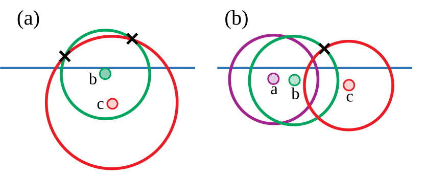
In this section, we prove that the left and right wavefronts we merge must intersect at one unique point. As before, we assume that the points are distinct. Consider any three points , , and from the same cell, in order of -coordinate. We consider the arcs formed by their -radius circles, forming a wavefront on the top border of the cell. We prove that the arc of can intersect at most one location in the union of arcs formed by and . Suppose that ’s arc intersects at least two locations in ’s arc. Take any two of these locations. They are part of the circle that forms ’s arc. This is a contradiction because it implies the circle forming ’s arc has larger radius than the circle forming ’s arc, as shown in Figure 12(a). Therefore ’s arc can intersect at most one location in ’s arc. A similar argument shows that ’s arc can intersect at most one location in ’s arc.
Now we need to prove that ’s arc cannot intersect both ’s arc and ’s arc. Without loss of generality, suppose that ’s arc intersects with ’s arc. Then, once ’s arc intersects with ’s arc, the rest of ’s arc must be in the interior of ’s arc, and thus below the union of ’s and ’s arcs above the horizontal line. The rest of ’s arc must be in the interior of ’s arc because is to the right of , and their arcs are formed by circles of the same radius. This is shown in Figure 12(b).
Applying the above argument to all possible choices of and in the left wavefront, and all possible choices of in the right wavefront implies that there can only be one intersection between the two wavefronts.