Reconfigurable Intelligent Surface Enabled IoT Networks in Generalized Fading Channels

?abstractname?

This paper studies an Internet-of-Things (IoT) network employing a reconfigurable intelligent surface (RIS) over generalized fading channels. Inspired by the promising potential of RIS-based transmission, we investigate a RIS-enabled IoT network with the source node employing a RIS-based access point. The system is modelled with reference to a receiver-transmitter pair and the Fisher-Snedecor $\mathcal{F}$ model is adopted to analyse the composite fading and shadowing channel. Closed-form expressions are derived for the system with regards to the average capacity, average bit error rate (BER) and outage probability. Monte-Carlo simulations are provided throughout to validate the results. The results investigated and reported in this study extend early results reported in the emerging literature on RIS-enabled technologies and provides a framework for the evaluation of a basic RIS-enabled IoT network over the most common multipath fading channels. The results indicate the clear benefit of employing a RIS-enabled access point, as well as the versatility of the derived expressions in analysing the effects of fading and shadowing on the network. The results further demonstrate that for a RIS-enabled IoT network, there is the need to balance between the cost and benefit of increasing the RIS cells against other parameters such as increasing transmit power, especially at low SNR and/or high to moderate fading/shadowing severity.

I Introduction

Reconfigurable intelligent surfaces (RIS) are one of the emerging technologies, aimed at enabling the concept of “smart radio environments” in beyond 5G communication networks. The idea behind such technologies is to control the propagation environment in order to improve signal quality and coverage [1, 2]. RISs are man-made surfaces of electromagnetic material that are electronically controlled with integrated electronics and have unique wireless communication capabilities [3]. RIS-based transmission schemes have several benefits and key features. Ideally, they are conceptualised to be nearly passive with dedicated energy sources, the surface can shape the wave incident upon it, they have full-band response and easily deployable on different surfaces like buildings, vehicles or indoor spaces. Additionally, they are not affected by receiver noise and have no power amplifiers, thus, they do not amplify nor introduce noise when reflecting signals [3, 4].

RIS-enabled applications have recently been investigated with respect to signal-to-noise ratio (SNR) maximisation [4], improving signal coverage [5], improving massive MIMO systems [6], beamforming optimisation [7, 8, 9], as well as multi-user networks[10]. On the other hand, important 5G and beyond technologies such as Internet-of-Things (IoT) devices are yet to be explored with respect to RIS-enabled schemes, even though the IoT paradigm has recently received much attention in the literature [11, 12, 13, 14, 15]. IoT devices take advantage of short communication ranges to reduce latency, while optimising spectrum efficiency and energy efficiency [16, 15, 17], which are parameters that can be further enhances with RIS-enabled technologies [3].

Regarding the channel characteristics, generalised fading distributions have been proposed that include or closely approximate the most common fading distributions as special cases [18, 19, 20, 21], thus providing ease and flexibility of analysis. For example, a wireless network over generalised $\alpha-\mu$ fading channels was studied for the particular cases of the Weibull, Nakagami$-m$ and Rayleigh channels in [22], while a network over generalized $\kappa-\mu$ fading for the special cases of the Rician, Nakagami-$m$ and Rayleigh channels was studied in [23]. More recently, it was shown in [24] that the Fisher-Snedecor $\mathcal{F}$ composite fading model outperforms most other generalized fading models because it provides accurate modeling and characterisation of the simultaneous occurrence of multipath fading and shadowing. Furthermore, the Fisher-Snedecor $\mathcal{F}$ model includes several fading distributions as special cases, such as Nakagami-$m$ ($m_{s}\rightarrow\infty$), Rayleigh ($m_{s}\rightarrow\infty,$ $m=1$) and one-sided Gaussian distribution ($m_{s}\rightarrow\infty,$ $m=\nicefrac{{1}}{{2}}$), while being more mathematically tractable. Thus, a key motivation for this study.

In light of the foregoing, this study seeks to contribute the following. The analysis of a RIS-based IoT network over composite fading and shadowing Fisher-Snedecor channels, where a reference source node employs a RIS configured access point for transmission. This allows for the derivation of expressions for three metrics of performance analysis, namely; the average capacity, the bit error rate (BER) and the outage probability of the system. To the best of our knowledge, this is the first analysis of a RIS-based IoT network over composite fading and shadowing. The expressions are derived in closed-form and Monte Carlo simulations are provided throughout to verify the accuracy of our analysis. Additionally, asymptotic expressions of the system metrics are derived and compared with the exact solutions. These expressions were shown to provide further insight to the network analysis, while more tractable analytically. The results indicate the clear benefit of employing a RIS-enabled access point, with regards to the average capacity, BER and outage probability, as well as the versatility of the derived expressions in analysing the effects of fading and shadowing on the network. The results further demonstrate that for a RIS-enabled IoT network, there is the need to balance between the cost and benefit of increasing the RIS cells against other parameters such as increasing transmit power, especially at low SNR and/or high to moderate fading/shadowing severity.

The paper is organised as follows. In Section II, we describe the system model under study. Thereafter, in Section III, we derive expressions for efficient computation of the average capacity, BER and outage probability of the system. Finally, in Sections IV and V, we present the results and outline the main conclusions, respectively.

II System Model

We consider a network of IoT nodes, as illustrated in Fig. 1. Each transmitter-receiver pair consists of a simple source node ($S$) and a destination node ($D$) for the transmitted information. The node $S$ is assumed to employ a RIS (consisting of passive reflector elements) in the form of an AP to communicate over the network. As shown in the block diagram, the RIS can be connected over a wired link or optical fiber for direct transmission from $S$, and can support transmission without RF processing. For the system considered, we assume an intelligent AP with the RIS having knowledge of channel phase terms, such that the RIS-induced phases can be adjusted to maximise the received SNR through appropriate phase cancellations and proper alignment of reflected signals from the intelligent surface.

The received signal at $D$ can be represented as

$$y_{D} =\left[\sum_{n=1}^{N}h_{D,n}e^{-j\phi_{n}}\right]x+w_{D},$$ (1)

where $x$ represents the transmitted signal by $S$ with power $P_{s}$ and $w_{D}$ the additive white Gaussian noise (AWGN) at $D$. Without loss of generality, we denote the power spectral density of the AWGN as $N_{0}$. The term $\phi_{n}$ in (1) is the reconfigurable phase induced by the $n$th reflector of the RIS, which through phase matching, the SNR of the received signals can be maximised. The term $h_{D,n}=\sqrt{g_{d,n}r_{d}^{-\beta}}$, is the channel coefficient from $S$-to-$D$ with distance $r_{d}$, path-loss exponent $\beta$ and channel gain $g_{d,n}$ modelled as independently distributed Fisher-Snedecor $\mathcal{F}$ RVs with the following PDF and CDF, respectively [24]

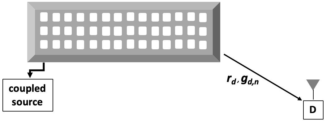
?figurename? 1: Source node RIS-based configuration employed as an access point.

$$f\left(g_{n}\right) =\Upsilon_{n}g_{n}^{-1}\textrm{G}_{1,1}^{1,1}\biggl{[}\Lambda_{n}\,g_{n}\Biggl{|}\negthickspace\begin{array}[]{c}1-m_{s_{n}}\\ m_{n}\end{array}\negthickspace\biggr{]},m_{s_{n}}>1,$$ (4)

and

$$F_{g_{n}}\left(v\right)=\Upsilon_{n}\,\textrm{G}_{2,2}^{1,2}\biggl{[}\Lambda_{n}v\Biggl{|}\negthickspace\begin{array}[]{c}1-m_{s_{n}},\,1\\ m_{n},\,0\end{array}\negthickspace\biggr{]},$$ (5)

where $n\in\left\{1,2,\ldots,N\right\}$, $\Upsilon_{n}=\frac{1}{\Gamma\left(m_{n}\right)\Gamma\left(m_{s_{n}}\right)}$ and $\Lambda_{n}=\frac{m_{n}}{\left(m_{s_{n}}-1\right)\bar{g}_{n}}$. The terms $\textrm{G}_{u,v}^{s,t}\left[\cdotp\right]$ is the Meijer’s G-function [25, Eq. (8.3.1.1)], $\Gamma\left(z\right)=\int_{0}^{\infty}t^{z-1}e^{-t}dt$ is the gamma function [26, Eq. (8.310)]and $\bar{g}_{n}=\mathbb{E}\left[g_{n}\right]$ is the mean power of the RV $g$ with $\mathbb{E}\left[\cdotp\right]$ denoting expectation. $m_{n}$ and $m_{s_{n}}$ represent the fading severity and shadowing parameters of the $n$-th RV, respectively.

Based on (1), the instanstaneous SNR at $D$ is given by

$$\gamma_{D}=\frac{\sum_{n=1}^{N}P_{s}\mid h_{D,n}\mid^{2}}{N_{0}}.$$ (6)

III Mathematical Analysis

In this section, we derive analytical expressions for various performance metrics of the system under consideration.

III-A Average Capacity Analysis

In this section, we derive analytical expressions for the average capacity over Fisher-Snedecor $\mathcal{F}$ composite fading. The capacity is defined by

$$C_{D}=\log_{2}\left(1+\gamma_{D}\right),$$ (7)

where $\gamma_{D}$ is the SNR at $D$.

The average capacity is given by

$$\overline{C}_{D} =\mathbb{E}\left[\log_{2}\left(1+\gamma_{D}\right)\right]$$

$$=\stackrel{{\scriptstyle[}}{{0}}]{\infty}{\int}\log_{2}\left(1+\frac{P_{s}r_{d}^{-\beta}}{N_{0}}g_{D}\right)f\left(g_{D}\right)\textrm{d}g_{D},$$ (8)

where $g_{D}=\sum_{n=1}^{N}g_{d,n}$. As can be observed, the RV $g_{D}$ is a sum of independent Fisher-Snedecor $\mathcal{F}$ distributed RVs, therefore, from (4) and [27, Eq. (7)], the PDF is given by

$$f\left(g\right)=\frac{1}{gB\left(Nm,Nm_{s}\right)}\left(\frac{gm}{Nm_{s}}\right)^{Nm}\\ \times{}_{\phantom{}2}F_{1}\left(N\left(m+m_{s}\right),Nm;Nm;-\frac{gm}{Nm_{s}}\right),$$ (9)

where ${}_{\phantom{}2}F_{1}\left(\alpha;\beta;\gamma;z\right)$ is the Gauss hypergeometric function [26, Eq. (9.111)] and $B\left(.,.\right)$ is the beta function [26, Eq. (8.384.1)]. To proceed, we express the PDF (9) in a more tractable form, by re-writing the PDF in an alternate form.

Using the relation $B\left(x,y\right)=\frac{\Gamma\left(x\right)\Gamma\left(y\right)}{\Gamma\left(x+y\right)}$ [26, Eq. (8.384.1)] and ${}_{\phantom{}2}F_{1}\left(\alpha;\beta;\gamma;-z\right)=\frac{\Gamma\left(\gamma\right)z}{\Gamma\left(\alpha\right)\Gamma\left(\beta\right)}\textrm{G}_{2,2}^{1,2}\left(z\Biggl{|}\negthickspace\begin{array}[]{c}-\alpha,\,-\beta\\ -1,\,-\gamma\end{array}\negthickspace\right)$ [26, Eq. (8.384.1)] with some algebraic manipulations, the PDF can be rewritten as

$$f\left(g\right)=\frac{g^{Nm}}{\Gamma\left(Nm\right)\Gamma\left(Nm_{s}\right)}\left(\frac{m}{Nm_{s}}\right)^{Nm+1}\\ \times\textrm{G}_{2,2}^{1,2}\left(\frac{gm}{Nm_{s}}\Biggl{|}\negthickspace\begin{array}[]{c}-N\left(m+m_{s}\right),\,-Nm\\ -1,\,-Nm\end{array}\negthickspace\right).$$ (10)

With the appropriate change of variables and representing the logarithmic function in terms of the Meijer G-function with the aid of [28, Eq. (11)], i.e.,

$$\textrm{ln}\left(1+z\right)=G_{2,2}^{1,2}\Bigl{[}z\Bigl{|}\!\begin{array}[]{c}1,1\\ 1,0\end{array}\!\Bigr{]},$$ (11)

we can re-express (8) as

$$\overline{C}_{D} =\frac{\Lambda}{\textrm{ln}\left(2\right)}\stackrel{{\scriptstyle[}}{{0}}]{\infty}{\int}g_{D}^{Nm}\,\textrm{G}_{2,2}^{1,2}\left(\eta g_{D}\biggl{|}\negthickspace\begin{array}[]{c}1,1\\ 1,0\end{array}\right)$$ (14)

$$\qquad\qquad\times\textrm{G}_{2,2}^{1,2}\left(\xi g_{D}\Biggl{|}\negthickspace\begin{array}[]{c}-N\left(m+m_{s}\right),\,-Nm\\ -1,\,-Nm\end{array}\negthickspace\right)\textrm{d}g_{D}.$$ (17)

$$\stackrel{{\scriptstyle\left(a\right)}}{{=}}\frac{\Lambda}{\textrm{ln}\left(2\right)}\stackrel{{\scriptstyle[}}{{0}}]{\infty}{\int}\textrm{G}_{2,2}^{1,2}\left(\eta g_{D}\biggl{|}\negthickspace\begin{array}[]{c}1,1\\ 1,0\end{array}\right)$$ (20)

$$\qquad\qquad\qquad\quad\times\textrm{G}_{2,2}^{1,2}\left(\xi g_{D}\Biggl{|}\negthickspace\begin{array}[]{c}-Nm_{s},\,0\\ Nm-1,\,0\end{array}\negthickspace\right)\textrm{d}g_{D},$$ (23)

where $\left(a\right)$ was obtained using [26, Eq. (9.31.5)]. The terms $\xi=\frac{m}{Nm_{s}}$ , $\eta=\frac{P_{s}r_{d}^{-\beta}}{N_{0}}$ and $\Lambda=\frac{\xi}{\Gamma\left(Nm\right)\Gamma\left(Nm_{s}\right)}.$

The integral in (23) can be evaluated using [26, Eq. (7.811.1)], to obtain the average capacity as

$$\overline{C}_{D}=\frac{\Lambda}{\xi\textrm{ln}\left(2\right)}\,\textrm{G}_{4,4}^{3,3}\biggl{[}\,\frac{\eta}{\xi}\biggl{|}\negthickspace\begin{array}[]{c}1-Nm,0,1,1\\ Nm_{s},0,1,0\end{array}\negthickspace\biggr{]}.$$ (24)

III-B Bit Error Rate Analysis

In this section, we analyse the BER over Fisher-Snedecor $\mathcal{F}$ composite fading. The average BER is defined as

$$\overline{P}_{e}=\stackrel{{\scriptstyle[}}{{0}}]{\infty}{\int}Q\left(\sqrt{2\eta\lambda g_{D}}\right)f\left(g_{D}\right)\textrm{d}g_{D},$$ (25)

where $Q\left(x\right)=\frac{1}{\sqrt{2\pi}}\stackrel{{\scriptstyle[}}{{x}}]{\infty}{\int}\exp\left(-\frac{u^{2}}{2}\right)$d$u$ is the Gaussian $Q$-function. The term $\lambda$ is a modulation constant, with $\lambda=\left\{0.5,1\right\}$ for binary frequency shift keying (BFSK) and binary phase shift keying (BPSK), respectively.

Using the relation $Q\left(x\right)=\frac{1}{2}\textrm{erfc}\left(\frac{x}{\sqrt{2}}\right)$, where $\textrm{erfc}\left(x\right)$ is the complementary error function and expressing the error function in terms of the Meijer G-function, i.e.,

$$\textrm{erfc}\left(\sqrt{z}\right)=\frac{1}{\sqrt{\pi}}G_{1,2}^{2,0}\Bigl{[}z\Bigl{|}\!\begin{array}[]{c}1\\ 0,0.5\end{array}\!\Bigr{]},$$ (26)

we can re-express (25) as

$$\overline{P}_{e} =\stackrel{{\scriptstyle[}}{{0}}]{\infty}{\int}\frac{1}{2}\textrm{erfc}\left(\sqrt{\eta\lambda g_{D}}\right)f\left(g_{D}\right)\textrm{d}g_{D}$$

$$\stackrel{{\scriptstyle\left(b\right)}}{{=}}\stackrel{{\scriptstyle[}}{{0}}]{\infty}{\int}\frac{\Lambda}{2\sqrt{\pi}}g_{D}^{Nm}G_{1,2}^{2,0}\left(\eta\lambda g_{D}\Bigl{|}\!\begin{array}[]{c}1\\ 0,0.5\end{array}\!\right)$$ (29)

$$\qquad\times\textrm{G}_{2,2}^{1,2}\left(\xi g_{D}\Biggl{|}\negthickspace\begin{array}[]{c}-N\left(m+m_{s}\right),\,-Nm\\ -1,\,-Nm\end{array}\negthickspace\right)\textrm{d}g_{D}.$$ (32)

$$\stackrel{{\scriptstyle\left(c\right)}}{{=}}\stackrel{{\scriptstyle[}}{{0}}]{\infty}{\int}\frac{\Lambda}{2\sqrt{\pi}}G_{1,2}^{2,0}\left(\eta\lambda g_{D}\Bigl{|}\!\begin{array}[]{c}1\\ 0,0.5\end{array}\!\right)$$ (35)

$$\qquad\times\textrm{G}_{2,2}^{1,2}\left(\xi g_{D}\Biggl{|}\negthickspace\begin{array}[]{c}-Nm_{s},\,0\\ Nm-1,\,0\end{array}\negthickspace\right)\textrm{d}g_{D},$$ (38)

where $\left(b\right)$ was obtained using (10) and (26), while $\left(c\right)$ was obtained using [26, Eq. (9.31.5)].

Using [26, Eq. (7.811.1)], the average BER can be obtained by evaluating the integral in (38) as

$$\overline{P}_{e}=\frac{\Lambda}{\eta\lambda 2\sqrt{\pi}}\,\textrm{G}_{4,3}^{1,4}\biggl{[}\,\frac{\xi}{\eta\lambda}\biggl{|}\negthickspace\begin{array}[]{c}0,-\frac{1}{2},-Nm_{s},0\\ Nm-1,0,-1\end{array}\negthickspace\biggr{]}.$$ (39)

III-C Outage Probability Analysis

In this section, we derive analytical expressions for the outage probability over Fisher-Snedecor $\mathcal{F}$ composite fading. The outage probability $P_{\textrm{out}}$, is defined as the probability that the received SNR falls below a certain threshold value denoted here as $\gamma_{\textrm{th}}$. For the considered network, the outage probability is given by

$$P_{\textrm{out}} =\Pr\left\{\gamma_{D}<\gamma_{\textrm{th}}\right\},$$

$$=\stackrel{{\scriptstyle[}}{{0}}]{\gamma_{\textrm{th}}}{\int}f\left(\gamma_{D}\right)\textrm{d}\gamma_{D}$$ (40)

where $\gamma_{D}$ is defined in (6). It can be observed that $\gamma_{D}$ follows a distribution of the sum of independent Fisher-Snedecor $\mathcal{F}$ distributed RVs, with the PDF $f\left(g_{D}\right)$ defined in (10). Then from (40), $P_{\textrm{out}}$ is the CDF of $\gamma_{D}$, which can be evaluated using [27, Eq. (9)] as

$$P_{\textrm{out}} =\frac{\Gamma\left(Nm+Nm_{s}\right)}{\Gamma\left(1+Nm\right)\Gamma\left(Nm_{s}\right)}\left(\frac{\gamma_{\textrm{th}}m}{\eta Nm_{s}}\right)^{Nm}$$

$$\times{}_{\phantom{}2}F_{1}\left(N\left(m+m_{s}\right),Nm;1+Nm;-\frac{\gamma_{\textrm{th}}m}{\eta Nm_{s}}\right),$$ (41)

where $\eta=\frac{P_{s}r_{d}^{-\beta}}{N_{0}}$. Note that (41) converges if $\mid\frac{\gamma_{\textrm{th}}m}{\eta Nm_{s}}\mid\><1$.

III-D Asymptotic Analysis

The asymptotic analysis is anchored in obtaining expressions in higher SNR regimes to gain further insight in the system performance. In this subsection, asymptotic expressions for the average capacity, average BER and outage probability will be derived.

III-D1 Average Capacity

The asymptotic capacity can be obtained to gain further insight at higher SNR regimes. When $g_{D}$ is sufficiently large, then $\ln\left(1+z\right)\simeq\ln\left(z\right).$ Next, from [27, Eq. (8)], we employ an alternative form of (9) for the PDF of $g_{D}$ given by

$$f\left(g\right)=\frac{\left(\frac{gm}{Nm_{s}}\right)^{Nm}}{gB\left(Nm,Nm_{s}\right)}\left(1+\frac{gm}{Nm_{s}}\right)^{-N\left(m+m_{s}\right)}.$$ (42)

Using the definition of the average capacity (8) and the PDF (42), the asymptotic capacity is given by

$$\overline{C}_{D}^{asy} =\stackrel{{\scriptstyle[}}{{0}}]{\infty}{\int}\log_{2}\left(\eta g_{D}\right)f\left(g_{D}\right)\textrm{d}g_{D},$$

$$=\frac{\left(\frac{m}{Nm_{s}}\right)^{Nm}}{\ln\left(2\right)B\left(Nm,Nm_{s}\right)}\stackrel{{\scriptstyle[}}{{0}}]{\infty}{\int}\frac{g_{D}^{Nm-1}\ln\left(\eta g_{D}\right)}{\left(1+\frac{g_{D}m}{Nm_{s}}\right)^{N\left(m+m_{s}\right)}}\textrm{d}g_{D}.$$ (43)

By using [29, Eq. (2.6.4.7)], the integral in (43) can be evaluated to obtain the asymptotic average capacity as

$$\overline{C}_{D}^{asy}\backsimeq\frac{\ln\left(\frac{\eta}{\xi}\right)+\psi\left(Nm\right)-\psi\left(Nm_{s}\right)}{\ln\left(2\right)},$$ (44)

where $\psi\left(z\right)=\frac{\textrm{d log}\left(\Gamma\left(z\right)\right)}{\textrm{d}z}$ is the psi function [26, Eq. (8.360.1)].

III-D2 Average BER

From (9), the PDF of $g_{D}$ at the origin can be expressed as

$$f\left(g\right)=\frac{g^{Nm-1}}{B\left(Nm,Nm_{s}\right)}\left(\frac{m}{Nm_{s}}\right)^{Nm},$$ (45)

where we have used the hypergeometric function identity ${}_{\phantom{}2}F_{1}\left(\alpha;\beta;\gamma;0\right)=1.$ Thus, from the definition of the average BER (25), (26) and the PDF (45), we can express the asymptotic BER as

$$\overline{P}_{e}^{asy} \backsimeq\frac{1}{2\sqrt{\pi}B\left(Nm,Nm_{s}\right)}\left(\frac{m}{Nm_{s}}\right)^{Nm}$$

$$\qquad\times\stackrel{{\scriptstyle[}}{{0}}]{\infty}{\int}g_{D}^{Nm-1}G_{1,2}^{2,0}\left(\eta\lambda g_{D}\Bigl{|}\!\begin{array}[]{c}1\\ 0,0.5\end{array}\!\right)\textrm{d}g_{D}.$$ (48)

Finally, the asymptotic BER can be obtained by evaluating the integral in (48), with the aid of [26, Eq. (7.811.4)], to obtain the expression as

$$\overline{P}_{e}^{asy}\backsimeq\frac{\Gamma\left(\frac{1}{2}+Nm\right)}{2\sqrt{\pi}B\left(Nm,Nm_{s}\right)Nm}\left(\frac{m}{\eta\lambda Nm_{s}}\right)^{Nm}.$$ (49)

III-D3 Outage Probability

The asymptotic outage probability can be obtained when $\frac{P_{s}}{N_{0}}\rightarrow\infty$. From (41), we invoke the identity ${}_{\phantom{}2}F_{1}\left(\alpha;\beta;\gamma;0\right)=1,$ (when $\eta\rightarrow\infty$) to obtain an asymptotic approximation as

$$P_{\textrm{out}}^{asy}\backsimeq\frac{\Gamma\left(Nm+Nm_{s}\right)}{\Gamma\left(1+Nm\right)\Gamma\left(Nm_{s}\right)}\left(\frac{\gamma_{\textrm{th}}m}{\eta Nm_{s}}\right)^{Nm},$$ (50)

where it can be readily observed that the diversity gain is equivalent to $Nm.$

It is worth noting that the asymptotic expressions for the capacity, BER and outage probability in (44), (49) and (50) respectively, have more tractable closed-forms that are easier for analysis. As will be demonstrated in the next section, these expressions closely approximate the exact solutions.

IV Numerical Results and Discussions

In this section, we present and discuss results from the mathematical expressions derived in the paper. We then investigate the effect of key parameters on the system. The results are then verified using Monte Carlo simulations with at least $10^{5}$ iterations. Unless otherwise stated, we have assumed RIS-to-$D$ distance has been normalised to unit distance, $r_{D}=1$ m, pathloss exponent $\beta=2.7$ and shadowing parameter $m_{s}=5$ (moderate).

In Fig. 2, we commence analysis for the IoT RIS-enabled network, with the average capacity against source power for different numbers of RIS cells and fading parameters. We consider fading parameters $m=1$ (heavy) and $m=4$ (moderate). It can be observed that the average capacity at a fixed SNR value, is proportional to the number of RIS cells. It can be further noted that within the region considered, the fading parameter has a far lesser effect on the average capacity compared to the source power and the number of RIS cells. Moreover, the asymptotic solution closely matches the exact solutions. An observation on doubling the number of cells from $N=16$ to 32 cells (at fixed transmission power) corresponds to about 1 bit/Hz increase in average capacity. Thus, from a design perspective, this may be insightful for a cost-benefit decision.

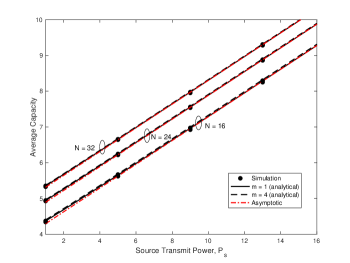
?figurename? 2: Average capacity versus source transmit power $P_{s}$ for the RIS-enabled access point node. Parameters considered with varying severity of fading parameter $m$ and number of RIS cells $N$.

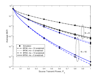
?figurename? 3: Average BER versus source transmit power $P_{s}$ for the RIS-enabled access point node. Parameters considered with varying severity of shadowing parameter $m_{s}$, number of RIS cells $N$ and modulation scheme.

Fig. 3 shows a plot of the average BER against source power for different numbers of RIS cells and fading parameters at very low SNR (maximum 0 dB). We consider modulating schemes $\lambda=0.5$ (BFSK) and $\lambda=1$ (BPSK). We assume fading parameters $m=1$. Overall, we observe that the average BER for both modulation schemes is lower with a higher number of RIS cells $N=16$, except at very low SNR, where BFSK $N=16,$ almost equal to best performing schemes for $N=8$ for BPSK. Additionally, the improvement in the error performance between the modulation schemes (and shadowing severities) is more noticeable with higher number of cells at $N=16.$ The results also demonstrates that the BPSK scheme performs better than BFSK for the different observed regions of shadowing severities, source transmit powers and number of RIS cells considered. We also note the clear benefit of employing the RIS schemes by observing that, by doubling the cells from $N=8$ to 16, we can achieve as an example, a BER improvement of about 3 orders of magnitude for BPSK $m_{s}=2.$ The knowledge of the effect of shadowing is particularly important in IoT networks, since it is possible for the shadowing severity on a device to rapidly change especially indoors.

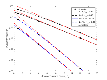
?figurename? 4: Outage probability versus the source transmit power $P_{s}$ for the RIS-enabled access point node. Parameters considered for different SNR threshold $\gamma_{\textrm{th}}$ and number of RIS cells $N$. Fixed values $m=1$ and $m_{s}=5.$

In Fig. 4, we present the outage probability against source transmit power for different number of RIS cells and SNR thresholds. We assume a fading severity $m=1$ and shadowing parameter $m_{s}=5$. It can be observed that for the number of RIS cells considered at different transmit powers, acceptable levels of outage probabilities can be achieved, even at low SNR regimes. It can be further observed that the benefit of the RIS configuration indicates that as low as 0 dB, an improvement of at least 5 orders of magnitude can be achieved by doubling the RIS cells from $N=8$ to 16, with further improvements for higher SNR levels. Meanwhile, increasing the desired SNR threshold by 3 orders of magnitude from $\gamma_{\textrm{th}}=3$ dB to 6 dB, corresponds to an approximate increase of 2 to 4 orders of magnitude in outage probability, which is in line with the diversity gain of $N*m$ as earlier discussed. Thus, considering the cost involved, it may be worth considering a transmit power increase, while adjusting the desired SNR threshold for an approximately similar benefit. Furthermore, plots of the asymptotic outage probability (obtained from (50)), demonstrate that for both RIS-conifigurations considered in Fig. 4, an SNR level of 9 dB to 10 dB is sufficient to allow convergence between the asymptotic approximation and exact analytical expression in (41).

V Conclusions

In this paper, we examined an IoT network employing a reconfigurable intelligent surface (RIS) over composite fading and shadowing channels. Exact expressions were derived for the efficient computation of system metrics such as the average capacity, average BER and outage probability, as well as approximate more tractable asymptotic expressions. The effects of parameters such as source transmit power, severity of fading and shadowing as well as number of RIS-cells were investigated. The results indicate the clear benefit of employing a RIS-enabled access point, with regards to the average capacity, BER and outage probability, as well as the versatility of the derived expressions in analysing the effects of fading and shadowing on the network. The results further demonstrate that for a RIS-enabled IoT network, there is the need to balance between the cost and benefit of increasing the RIS cells against other parameters such as increasing transmit power, especially at low SNR and/or high to moderate fading/shadowing severity.

- [1] M. D. Renzo, M. Debbah, D.-T. Phan-Huy, A. Zappone, M.-S. Alouini, C. Yuen, V. Sciancalepore, G. C. Alexandropoulos, J. Hoydis, H. Gacanin, J. d. Rosny, A. Bounceur, G. Lerosey, and M. Fink, “Smart radio environments empowered by reconfigurable AI meta-surfaces: An idea whose time has come,” EURASIP J. Wireless Commun. Netw., vol. 2019, no. 1, p. 129, May 2019. [Online]. Available: https://doi.org/10.1186/s13638-019-1438-9
- [2] C. Liaskos, S. Nie, A. Tsioliaridou, A. Pitsillides, S. Ioannidis, and I. Akyildiz, “A new wireless communication paradigm through software-controlled metasurfaces,” IEEE Communications Magazine, vol. 56, no. 9, pp. 162–169, Sep. 2018.
- [3] E. Basar, M. D. Renzo, J. D. Rosny, M. Debbah, M.-S. Alouini, and R. Zhang, “Wireless communications through reconfigurable intelligent surfaces,” IEEE Access, vol. 7, pp. 116 753–116 773, 2019.
- [4] E. Basar, “Transmission Through Large Intelligent Surfaces: A New Frontier in Wireless Communications,” in 2019 European Conf. Netw. Commun. (EuCNC), Jun. 2019, pp. 112–117.
- [5] L. Subrt and P. Pechac, “Controlling propagation environments using intelligent walls,” in 6th European Conf. Antennas Propag. (EUCAP), Mar. 2012, pp. 1–5.
- [6] S. Hu, F. Rusek, and O. Edfors, “Beyond Massive MIMO: The Potential of Data Transmission With Large Intelligent Surfaces,” IEEE Trans. Sig. Process., vol. 66, no. 10, pp. 2746–2758, May 2018.
- [7] Q. Wu and R. Zhang, “Beamforming optimization for intelligent reflecting surface with discrete phase shifts,” in IEEE Int. Conf. Acoust., Speech and Sig. Process. (ICASSP), May 2019, pp. 7830–7833.
- [8] ——, “Intelligent reflecting surface enhanced wireless network: Joint active and passive beamforming design,” in IEEE Global Commun. Conf. (GLOBECOM), Dec 2018, pp. 1–6.
- [9] X. Tan, Z. Sun, J. M. Jornet, and D. Pados, “Increasing indoor spectrum sharing capacity using smart reflect-array,” in IEEE Int. Conf. Commun. (ICC), May 2016, pp. 1–6.
- [10] C. Huang, A. Zappone, M. Debbah, and C. Yuen, “Achievable Rate Maximization by Passive Intelligent Mirrors,” in IEEE Int. Conf. Acoust. Speech Sig. Process. (ICASSP), Apr. 2018, pp. 3714–3718.
- [11] S. J. Ambroziak, L. M. Correia, R. J. Katulski, M. Mackowiak, C. Oliveira, J. Sadowski, and K. Turbic, “An Off-Body Channel Model for Body Area Networks in Indoor Environments,” IEEE Trans. Antennas Propag., vol. 64, no. 9, pp. 4022–4035, Sep. 2016.
- [12] S. Kumar, U. Dohare, K. Kumar, D. Prasad, K. N. Qureshi, and R. Kharel, “Cybersecurity measures for geocasting in vehicular cyber physical system environments,” IEEE Internet Things J., pp. 1–1, 2019.
- [13] R. Kasana, S. Kumar, O. Kaiwartya, R. Kharel, J. Lloret, N. Aslam, and T. Wang, “Fuzzy-based channel selection for location oriented services in multichannel VCPS environments,” IEEE Internet Things J., vol. 5, no. 6, pp. 4642–4651, Dec 2018.
- [14] Z. Kuang, G. Liu, G. Li, and X. Deng, “Energy Efficient Resource Allocation Algorithm in Energy Harvesting-Based D2D Heterogeneous Networks,” IEEE Internet Things J., vol. 6, no. 1, pp. 557–567, Feb 2019.
- [15] M. M. Elmesalawy, “D2D communications for enabling internet of things underlaying LTE cellular networks,” J. Wireless Netw. Commun., vol. 6, no. 1, pp. 1–9, 2016.
- [16] J. H. Anajemba, Y. Tang, J. A. Ansere, and C. Iwendi, “Performance analysis of D2D energy efficient IoT networks with relay-assisted underlaying technique,” in Proc. 44th IEEE Annual Conf. Ind. Electron. Soc. (IECON), Oct. 2018, pp. 3864–3869.
- [17] W. Stallings, Foundations of Modern Networking: SDN, NFV, QoE, IoT and Cloud. Addison-Wesley Professional, 2015.
- [18] M. D. Yacoub, “The - distribution: A general fading distribution,” in Proc. IEEE Annual Int. Symp. Personal, Indoor, and Mobile Radio Commun. (PIMRC), vol. 2, Sept. 2002, pp. 629–633.
- [19] ——, “The - distribution: A general fading distribution,” in Proc. IEEE Veh. Technology Conf. (VTC-Fall), vol. 2, Sept. 2000, pp. 872–877.
- [20] ——, “The - distribution: A general fading distribution,” in Proc. IEEE Veh. Technology Conf. (VTC-Fall), vol. 3, Oct. 2001, pp. 1427–1431.
- [21] X. Li, J. Li, L. Li, J. Jin, J. Zhang, and D. Zhang, “Effective Rate of MISO Systems over - Shadowed Fading Channels,” IEEE Access, vol. 5, pp. 10 605–10 611, 2017.
- [22] G. Nauryzbayev, K. M. Rabie, M. Abdallah, and B. Adebisi, “On the performance analysis of WPT-based dual-hop AF relaying networks in - fading,” IEEE Access, vol. 6, pp. 37 138–37 149, 2018.
- [23] K. Rabie, B. Adebisi, G. Nauryzbayev, O. S. Badarneh, X. Li, and M. Alouini, “Full-duplex energy-harvesting enabled relay networks in generalized fading channels,” IEEE Wireless Commun. Lett., vol. 8, no. 2, pp. 384–387, Apr. 2018.
- [24] S. K. Yoo, S. L. Cotton, P. C. Sofotasios, M. Matthaiou, M. Valkama, and G. K. Karagiannidis, “The Fisher-Snedecor distribution: A simple and accurate composite fading model,” IEEE Commun. Lett., vol. 21, no. 7, pp. 1661–1664, Jul. 2017.
- [25] A. P. Prudnikov, Y. A. Brychkov, and O. I. Marichev, Integrals, and Series: More Special Functions, Gordon and Breach Sci. Publ., New York, 1990, vol. 3.
- [26] I. S. Gradshteyn and I. M. Ryzhik, Table of Integrals, Series, and Products, 7th ed. Academic Press, Califonia, 2007.
- [27] O. S. Badarneh, D. B. da Costa, P. C. Sofotasios, S. Muhaidat, and S. L. Cotton, “On the sum of fisher-snedecor F variates and its application to maximal-ratio combining,” 2019.
- [28] V. S. Adamchik and O. I. Marichev, “The algorithm for calculating integrals of hypergeometric type functions and its realization in reduce systems,” in Proc. Int. Conf. on Symbolic and Algebraic Comput., 1990, pp. 212–224.
- [29] A. P. Prudnikov, Y. A. Brychkov, and O. I. Marichev, Integrals and Series: Elementary Functions, Gordon and Breach Sci. Publ., New York, 1998, Vol. 1.