Fast non-convex low-rank matrix decomposition for separation of potential field data using minimal memory

Abstract.

A fast non-convex low-rank matrix decomposition method for potential field data separation is proposed. The singular value decomposition of the large size trajectory matrix, which is also a block Hankel matrix, is obtained using a fast randomized singular value decomposition algorithm in which fast block Hankel matrix-vector multiplications are implemented with minimal memory storage. This fast block Hankel matrix randomized singular value decomposition algorithm is integrated into the Altproj algorithm, which is a standard non-convex method for solving the robust principal component analysis optimization problem. The improved algorithm avoids the construction of the trajectory matrix. Hence, gravity and magnetic data matrices of large size can be computed. Moreover, it is more efficient than the traditional low-rank matrix decomposition method, which is based on the use of an inexact augmented Lagrange multiplier algorithm. The presented algorithm is also robust and, hence, algorithm-dependent parameters are easily determined. The improved and traditional algorithms are contrasted for the separation of synthetic gravity and magnetic data matrices of different sizes. The presented results demonstrate that the improved algorithm is not only computationally more efficient but it is also more accurate. Moreover, it is possible to solve far larger problems. As an example, for the adopted computational environment, matrices of sizes larger than $205\times 205$ generate “out of memory” exceptions with the traditional method, but a matrix of size $2001\times 2001$ can be calculated in $1062.29$s with the new algorithm. Finally, the improved method is applied to separate real gravity and magnetic data in the Tongling area, Anhui province, China. Areas which may exhibit mineralizations are inferred based on the separated anomalies.

Dan Zhu

Institude of Geophysics & Geomatics

China University of Geosciences (Wuhan)

Wuhan, MO 430074, China

Rosemary A. Renaut^∗

School of Mathematical and Statistical Sciences

Arizona State University

Tempe, MO 85287, USA

Hongwei Li and Tianyou Liu

Institude of Geophysics & Geomatics

China University of Geosciences (Wuhan)

Wuhan, MO 430074, China

1. Introduction

To study target geological sources, the target gravity, or magnetic anomalies, that are caused by the target sources, should be separated from the total fields which are the superposition of the gravity and magnetic fields caused by all underground sources. Separated anomalies are then used for data inversion and interpretation of geological features. Therefore, the separation of potential field data is an important step for high quality inversion and interpretation. Deep sources generate large scale smooth anomalies which are called regional anomalies. Residual anomalies, which are on a small scale, are caused by shallow sources. There are many methods for separating the regional-residual anomalies. They can be classified into three types. The classical methods of the first group separate the data in the spatial domain. These include methods such as the moving average, polynomial fitting, minimum curvature, and empirical mode decomposition, [22, 1, 16, 15]. Methods of the second and third types separate the anomalies in the frequency or wavelet domains, respectively. These include methods such as matched filtering, Wiener filtering, continuation, and discrete wavelet analysis, [5, 18, 20, 19, 6]. While algorithms that separate the anomalies in the frequency or wavelet domains are easy to implement [9, 27], the spectral overlapping of the regional and residual anomalies makes it difficult to obtain satisfactory results [28].

It has been demonstrated in areas of image and signals processing that the use of a low-rank matrix decomposition for robust principal component analysis (RPCA) is very effective [4]. The fundamental observation is that practical data from applied science fields is usually distributed on low-dimensional manifolds in high-dimensional spaces [13]. The mathematical model for RPCA is a double-objective optimization that separates the matrix into a low-rank matrix and a sparse matrix. Because RPCA is robust and provides high accuracy separation, it has been applied in many fields, and there is much research on solving the optimization problem. Generally, the Lagrange function is used to transform the double-objective optimization problem into a single-objective optimization problem that is solved using convex optimization. Iterative thresholding, accelerated proximal gradient, exact augmented Lagrange multiplier (EALM), and inexact augmented Lagrange multiplier (IALM) algorithms have been proposed to solve the convex optimization problem [26, 2, 12]. Due to the high computational cost of convex RPCA, a non-convex RPCA algorithm, which is called Altproj, has been proposed to reduce the cost [17]. Furthermore, as compared with convex RPCA, the higher accuracy of Altproj has lead to its wide adoption.

A low-rank matrix decomposition algorithm for potential field separation (LRMD_PFS), based on RPCA and singular spectrum analysis, has been proposed [29]. Singular spectrum analysis is a classical method using the trajectory matrix and the singular value decomposition (SVD) [21, 3, 23]. An important step in LRMD_PFS is the construction of the trajectory matrix (which is a block Hankel matrix) of the total field. Then, the trajectory matrix of the total field can be separated into a low-rank matrix and a sparse matrix using convex RPCA. The separated low-rank and sparse matrices are the approximations of the trajectory matrices of the regional anomalies and the residual anomalies, respectively. The sparse features of the regional anomalies in the frequency domain, and the localization features of the residual anomalies in the spatial domain, are both considered in LRMD_PFS. Although LRMD_PFS separates the anomalies without the use of a Fourier transform to the frequency domain, it can also be seen as providing a new group of methods because it provides a combination of the features of the potential field data in both spatial and frequency domains. Hence, as compared to classical methods, LRMD_PFS is more robust and has higher accuracy. The computational cost of LRMD_PFS is, however, high. There is a large memory demand associated with generating and storing the large scale trajectory matrix, and a large number of operations are required to generate the SVD of a large matrix. For example, if the size of the matrix is $101\times 101$, then the size of the constructed trajectory matrix is $2601\times 2601$. The trajectory matrix then requires memory that is $663$ times that of the original data. For a matrix of size $201\times 201$, the size of the trajectory matrix is $10201\times 10201$, and the memory demand increases by a factor of almost $2576$. Therefore, the size of the trajectory matrix increases rapidly with the size of the original matrix.

In this paper, a fast block Hankel matrix randomized SVD (FBHMRSVD) algorithm that requires minimal memory storage is proposed. FBHMRSVD is based on fast block Hankel matrix-vector multiplications (FBHMVM) [25, 14] and the use of a randomized SVD (RSVD) [11, 10, 24]. This then yields a fast non-convex low-rank matrix decomposition for potential field separation (FNCLRMD_PFS) that is based on the FBHMRSVD. FBHMRSVD is used to approximate the SVD of the trajectory matrix without constructing the large trajectory matrix. Further, implementing FBHMRSVD within Altproj also yields approximation of the trajectory matrices of the regional anomalies and residual anomalies without explicit construction of the trajectory matrix. Therefore, the large scale potential field data matrix can be separated using FNCLRMD_PFS. Furthermore, FNCLRMD_PFS has lower computational cost and higher accuracy than LRMD_PFS. The algorithm is developed and then contrasted with the classical approach for separation of synthetic data sets in Sections 2-4. Results showing that the algorithm efficiently and effectively separates real gravity and magnetic data in the Tongling area, Anhui province, China are presented in Section 5.

2. The Fast block Hankel matrix randomized singular value decomposition: FBHMRSVD

2.1. Fast block Hankel matrix-vector multiplication: FBHMVM

Consider a $2$D gridded potential field data matrix $\mathbf{X}=[x_{mn}]\in\mathcal{R}^{P\times Q}$, where $x_{mn}$ denotes the element at the $m$th row and $n$th column of the matrix $\mathbf{X}$. Before constructing the trajectory matrix, the Hankel matrix $\mathbf{T}_{j}$ is constructed using the $j$th column of $\mathbf{X}$ as follows,

$$\mathbf{T}_{j}=\begin{bmatrix}x_{1j}&x_{2j}&\dotsm&x_{(P-K+1)j}\\ x_{2j}&x_{3j}&\dotsm&x_{(P-K+2)j}\\ \vdots&\vdots&&\vdots\\ x_{Kj}&x_{(K+1)j}&\dotsm&x_{Pj}\end{bmatrix}.$$

Here, generally, $K=\lfloor(P+1)/2\rfloor$, where $\lfloor\>\rfloor$ denotes the integer part of its argument. If $\mathbf{T}_{j}$ has size $K\times L$, then $L=P-K+1$, and trajectory matrix $\mathbf{T}$ of size $K\hat{K}\times L(Q-\hat{K}+1)$ is constructed as follows,

$$\mathbf{T}=\begin{bmatrix}\mathbf{T}_{1}&\mathbf{T}_{2}&\dotsm&\mathbf{T}_{Q-\hat{K}+1}\\ \mathbf{T}_{2}&\mathbf{T}_{3}&\dotsm&\mathbf{T}_{Q-\hat{K}+2}\\ \vdots&\vdots&&\vdots\\ \mathbf{T}_{\hat{K}}&\mathbf{T}_{\hat{K}+1}&\dotsm&\mathbf{T}_{Q}\end{bmatrix}.$$

Setting $\hat{K}=\lfloor(Q+1)/2\rfloor$ makes $\mathbf{T}$ as near to square as possible. $\mathbf{T}$ is a block Hankel matrix with $\hat{K}\times\hat{L}$ blocks, where $\hat{L}=Q-\hat{K}+1$. The construction of $\mathbf{T}$ from $\mathbf{X}$ is denoted by

(1) $$\mathbf{T}=\mathcal{H}(\mathbf{X}).$$

Now, given a block Hankel matrix, efficient evaluation of matrix-vector products

(2) $$\mathbf{y}=\mathbf{T}\mathbf{b},$$

is required. Direct evaluation of the matrix-vector product using first (1) to find $\mathbf{T}$ and then calculating (2), uses approximately $8K\hat{K}L\hat{L}-K\hat{K}-L\hat{L}$ flops and requires storage of $K\hat{K}L\hat{L}+K\hat{K}+L\hat{L}$ floating point entries. On the other hand, using Algorithm 1, $\mathbf{y}$ can be calculated from $\mathbf{X}$ and $\mathbf{b}$ without constructing $\mathbf{T}$ using $\mathcal{O}(PQ\log_{2}{PQ})$ flops and a storage requirement of $3PQ+K\hat{K}+L\hat{L}$ entries. Here, the fast operation that combines (1) and (2) is detailed in Algorithm 1, and is denoted by

$$\mathbf{y}=\mathtt{FBHMVM}(\mathbf{X},\mathbf{b},K,\hat{K}).$$

Algorithm 1 Fast block Hankel matrix-vector multiplication: $\mathbf{y}=\mathtt{FBHMVM}(\mathbf{X},\mathbf{b},K,\hat{K})$.

1:  Input: potential field data matrix $\mathbf{X}\in\mathcal{R}^{P\times Q}$; vector $\mathbf{b}$.

2:  $\hat{\mathbf{W}}=\mathtt{ifft}2(\mathtt{fft}2(\mathbf{T}^{circ}).*\mathtt{fft}2(\mathbf{W}))$.

3:  Output: $\mathbf{y}=\mathbf{J}\mathtt{vec}(\mathtt{extract}(\hat{\mathbf{W}}))$.

Algorithm 1 uses the exchange matrix $\mathbf{J}$. This is the permutation matrix which is $0$ everywhere except for $1$s on the counter diagonal. It is also referred to as the reversal matrix, backward identity, or standard involutory permutation matrix. $\mathbf{T}^{circ}$ is defined by

$$\mathbf{T}^{circ}=\begin{bmatrix}\hat{\mathbf{T}}_{\hat{K}}&\dotsm&\hat{\mathbf{T}}_{1}&\hat{\mathbf{T}}_{\hat{L}}&\dotsm&\hat{\mathbf{T}}_{2}\end{bmatrix},$$

where $\hat{\mathbf{T}}_{j}$ is embedded from the $j$th column of $\mathbf{X}$ as follows,

$$\hat{\mathbf{T}}_{j}=\begin{bmatrix}x_{Kj}&\dotsm&x_{1j}&x_{Lj}&\dotsm&x_{2j}\end{bmatrix}^{T}.$$

$\mathbf{W}$ is constructed from $\mathbf{b}$ as follows,

$$\mathbf{W}=\begin{bmatrix}\mathbf{B}&\mathbf{0}_{L(\hat{L}-1)}\ \\ \mathbf{0}_{(L-1)\hat{L}}&\mathbf{0}_{(L-1)(\hat{L}-1)}\end{bmatrix}^{T}.$$

where $\mathbf{b}=\mathtt{vec}(\mathbf{B})$, and the operation $\mathtt{vec}(\cdot)$ denotes the vectorization operation. Moreover, the extraction operation is defined by

$$\mathtt{extract}(\hat{\mathbf{W}})=\hat{\mathbf{W}}(1:L,1:\hat{L}).$$

2.2. Fast block Hankel matrix-matrix multiplication: FBHMMM

It is immediate that Algorithm 1 can be extended for block Hankel matrix-matrix multiplication

$$\mathbf{Y}=\mathbf{T}\mathbf{C},$$

where the size of $\mathbf{C}$ is $P_{C}\times Q_{C}$. The process is given in Algorithm 2, and is denoted by

$$\mathbf{Y}=\mathtt{FBHMMM}(\mathbf{X},\mathbf{C},K,\hat{K}).$$

Algorithm 2 Fast block Hankel matrix-matrix multiplication: $\mathbf{Y}=\mathtt{FBHMMM}(\mathbf{X},\mathbf{C},K,\hat{K})$.

1:  Input: potential field data matrix $\mathbf{X}\in\mathcal{R}^{P\times Q}$; matrix $\mathbf{C}\in\mathcal{R}^{P_{C}\times Q_{C}}$; parameters $K$ and $\hat{K}$.

2:  for $j=1:Q_{C}$. do

3:     $\mathbf{Y}(:,j)=\mathtt{FBHMVM}(\mathbf{X},\mathbf{C}(:,j),K,\hat{K})$.

4:  end for

5:  Output: $\mathbf{Y}$.

2.3. The fast block Hankel matrix randomized SVD: FBHMRSVD

The SVD is the basis of matrix rank reduction, and it is an important step in RPCA. The process of the SVD for the block Hankel matrix is represented by

$$[\mathbf{U},\mathbf{\Sigma},\mathbf{V}]=\mathtt{SVD}(\mathcal{H}(\mathbf{X})).$$

Here $\mathbf{U}=[\mathbf{u}_{1},\mathbf{u}_{2},\dotsm]$ and $\mathbf{V}=[\mathbf{v}_{1},\mathbf{v}_{2},\dotsm]$ are unitary matrices, $\mathbf{u}_{1},\mathbf{u}_{2},\dotsm$ are left singular vectors, $\mathbf{v}_{1},\mathbf{v}_{2},\dotsm$ are right singular vectors; and $\mathbf{\Sigma}=\mathtt{diag}(\sigma_{1}^{2},\sigma_{2}^{2},\dotsm)$ is a diagonal matrix where $\sigma_{1}\geqslant\sigma_{2}\geqslant\dotsm\geqslant 0$ are the singular values of $\mathbf{T}$, and

$$\mathbf{T}=\mathbf{U}\mathbf{\Sigma}\mathbf{V}^{T}.$$

The cost of obtaining all terms of the SVD is $\mathcal{O}((L\hat{L})(K\hat{K})^{2})$, [7], which can be prohibitive when $P$ and $Q$ are large. For the rank reduction problem, however, not all terms are required and it can be sufficient to obtain a partial SVD with $r$ terms, corresponding to using a rank $r$ approximation,

(3) $$\mathbf{T}_{r}=\mathbf{U}_{r}\mathbf{\Sigma}_{r}\mathbf{V}_{r}^{T},$$

where $\mathtt{rank}(\mathbf{T}_{r})=r$. Generally, low-rank features of $\mathbf{T}$ are required and so $r$ is relatively small. Still, the cost of finding the exact dominant $r$ terms in (3) is high. On the other hand, the randomized singular value decomposition (RSVD), [11, 10], has been proposed for efficient determination of a low rank matrix approximation $\mathbf{T}_{r}$ without the exact calculation of the components in (3). Here, we implement the RSVD by taking advantage of all steps employing matrix-matrix multiplications with $\mathbf{T}$ using Algorithm 2, and without explicitly obtaining $\mathbf{T}$. This process, given in Algorithm 3, is denoted by

$$[\mathbf{U}_{r},\mathbf{\Sigma}_{r},\mathbf{V}_{r}]=\mathtt{FBHMRSVD}(\mathbf{X},K,\hat{K},r,p,q).$$

The integer parameters $p$, and $q$ are integral to the implementation of an RSVD algorithm. They represent an oversampling and power iteration parameter, respectively. When the required rank $r$ is relatively small with respect to the full rank of the matrix, it is sufficient to take $p=r$. While the accuracy of RSVD increases with increasing $q$, the cost also increases. But if the spectrum separates into a dominant larger set of values with $\sigma_{\ell}\gg\sigma_{\ell+1}$, it is sufficient to use a relatively small $q$, such as $q=0$, $1$ or $2$, where $q>0$ applies $q$ steps of a power iteration to improve the approximation to the dominant singular values.

Algorithm 3 Fast block Hankel matrix RSVD: $[\mathbf{U}_{r},\mathbf{\Sigma}_{r},\mathbf{V}_{r}]=\mathtt{FBHMRSVD}(\mathbf{X},K,\hat{K},r,p,q)$.

1:  Input: potential field data matrix $\mathbf{X}\in\mathcal{R}^{P\times Q}$; desired rank $r$; oversampling parameter $p$; power iteration parameter $q$; parameter $K$ and $\hat{K}$.

2:  $\ell=r+p$, $k=0$.

3:  Generate a Gaussian random matrix $\mathbf{\Omega}\in\mathcal{R}^{\ell\times K\hat{K}}$.

4:   $\mathbf{A}^{(0)}=\mathtt{FBHMMM}(\mathbf{X},\mathbf{\Omega}^{T},L,\hat{L})$.

5:  QR factorization: $[\mathbf{Q}^{(0)},\sim]=\mathtt{qr}(\mathbf{A}^{(0)})$, where $\mathbf{Q}^{(0)}\in\mathcal{R}^{L\hat{L}\times\ell}$ is an orthonormal matrix.

6:  while $q>k$ do

7:     $\mathbf{A}^{(1)}=\mathtt{FBHMMM}(\mathbf{X},\mathbf{\mathbf{Q}}^{(0)},K,\hat{K})$.

8:     $[\mathbf{Q}^{(1)},\sim]=\mathtt{qr}(\mathbf{A}^{(1)})$.

9:     $\mathbf{A}^{(2)}=\mathtt{FBHMMM}(\mathbf{X},\mathbf{\mathbf{Q}}^{(1)},L,\hat{L})$.

10:     $[\mathbf{Q}^{(2)},\sim]=\mathtt{qr}(\mathbf{A}^{(2)})$.

11:     $\mathbf{Q}^{(0)}=\mathbf{Q}^{(2)},k=k+1$.

12:  end while

13:  $\mathbf{B}=\mathtt{FBHMMM}(\mathbf{X},\mathbf{\mathbf{Q}}^{(0)},K,\hat{K})$.

14:  Compute the eigen-decomposition of $\mathbf{B}^{T}\mathbf{B}$: $[\tilde{\mathbf{V}}_{\ell},\mathbf{D}_{\ell}]=\mathtt{eig}(\mathbf{B}^{T}\mathbf{B})$.

15:  $\mathbf{V}_{r}=\mathbf{Q}^{(0)}\tilde{\mathbf{V}}_{\ell}(:,1:r)$; $\mathbf{\sigma}_{r}=\sqrt{\mathbf{D}_{\ell}(1:r,1:r)}$; $\mathbf{U}_{r}=\mathbf{B}\tilde{\mathbf{V}}_{\ell}(:,1:r)\mathbf{\Sigma}_{r}^{-1}$.

16:  Output: $\mathbf{U}_{r}$, $\mathbf{\Sigma}_{r}$, $\mathbf{V}_{r}$.

In Algorithm 3, note that steps 4, 7, 9, and 13 involve trajectory matrix-matrix multiplications and are replaced by the use of Algorithm 2 in order to avoid calculation of $\mathbf{T}$. The original equations are

$$\mathbf{A}^{(0)}=\mathbf{T}^{T}\mathbf{\Omega}^{T},\quad\mathbf{A}^{(1)}=\mathbf{T}\mathbf{Q}^{(0)},\quad\mathbf{A}^{(2)}=\mathbf{T}^{T}\mathbf{Q}^{(1)}\text{ and }\mathbf{B}=\mathbf{T}\mathbf{Q}^{(0)},$$

where $\mathbf{A}^{(0)}$, $\mathbf{A}^{(2)}\in\mathcal{R}^{L\hat{L}\times\ell}$ and $\mathbf{A}^{(1)}$, $\mathbf{Q}^{(1)}$, $\mathbf{B}\in\mathcal{R}^{K\hat{K}\times\ell}$. Because Algorithm 3 can be recast without using Algorithm 2 for matrix-matrix multiplications, the accuracy of the two algorithms is the same, up to floating point arithmetic errors that may accrue. But the computational cost is much reduced. The computational cost in terms of flops and storage for each algorithm are detailed, for each step, in Table 1. The storage and flops required for steps 5, 8, 10, 14, and 15 are the same. For $K\hat{K}L\hat{L}\gg PQ$, however, these costs are far lower in steps 4, 7, 9, and 13 when implemented using Algorithm 2.

Table 1. The computational cost measured in terms of floating point operations and storage of floating point entries at each step of Algorithm 3 implemented with (FBHMRSVD), and without (RSVD), the use of FBHMMM for multiplications with $\mathbf{T}$.

	FBHMRSVD		RSVD
Step	Cost in flops	Cost in storage	Cost in flops	Cost in storage
4, 9	$\mathcal{O}(\ell PQ\log_{2}{PQ})$	$PQ+\ell K\hat{K}+\ell L\hat{L}$	$2\ell K\hat{K}L\hat{L}$	$K\hat{K}L\hat{L}+\ell K\hat{K}+\ell L\hat{L}$
5, 10	$2\ell^{2}(L\hat{L}-\ell/3)$	$2\ell L\hat{L}$	$2\ell^{2}(L\hat{L}-\ell/3)$	$2\ell L\hat{L}$
7, 13	$\mathcal{O}(\ell PQ\log_{2}{PQ})$	$PQ+\ell K\hat{K}+\ell L\hat{L}$	$4\ell K\hat{K}L\hat{L}$	$K\hat{K}L\hat{L}+\ell K\hat{K}+\ell L\hat{L}$
8	$2\ell^{2}(K\hat{K}-\ell/3)$	$2\ell K\hat{K}$	$2\ell^{2}(K\hat{K}-\ell/3)$	$2\ell K\hat{K}$
14	$\mathcal{O}(\ell^{3})$	$2\ell^{2}+\ell$	$\mathcal{O}(\ell^{3})$	$2\ell^{2}+\ell$
15	$\ell r(2\ell+3K\hat{K})$	$r(K\hat{K}+L\hat{L})+2\ell^{2}$	$\ell r(2\ell+3K\hat{K})$	$r(K\hat{K}+L\hat{L})+2\ell^{2}$
		$+\ell L\hat{L}+r+\ell$		$+\ell L\hat{L}+r+\ell$

2.4. Experiments on FBHMRSVD

We now discuss the influence of the parameters on the accuracy and computational costs of Algorithm 3. We compare the computational costs with, and without, the use of Algorithm 2 for matrix multiplication, and the accuracy as compared to the use of the partial SVD. Hence, computations reported using RSVD and partial SVD are all based on the constructions of the trajectory matrices. The CPU of the computer for the computations in this paper is the Intel(R) Xeon (R) Gold 6138 CPU @ 2.00GHz; the release of MATLAB is 2019b.

First, we discuss the influence of the parameters on the computational cost and accuracy of Algorithm 3. Figure 1 shows the influence of the parameter $q$ on different sizes of the matrix $\mathbf{X}$, for $r=10$ and $q=0$, $1$ and $2$. The improvement in reducing the root mean square error (RMSE), which is defined by $\|\mathbf{X}^{*}-\hat{\mathbf{X}}\|_{2}/PQ$ where $\mathbf{X}^{*}$ and $\hat{\mathbf{X}}$ are the rank-$r$ approximations of $\mathbf{X}$ using the full SVD and Algorithm 3, respectively, is most significant when one power iteration is introduced, $q=1$. With larger $q$ the computational cost increases, as can be seen from Figure 1, demonstrating that the cost more than doubles when going from $q=0$ to $q=1$, but does not quite double again going from $q=1$ to $q=2$. Clearly there is a trade off between cost and accuracy, thus we recommend $q=1$ as a suitable compromise.

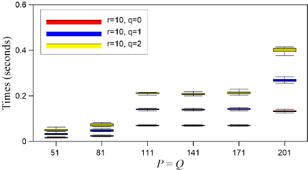
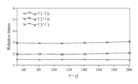
Figure 1. Experiments for Algorithm 3 for $r=10$ with $q=0$, $1$, $2$, and increasing $P=Q$. Each experiment is repeated $10$ times for each parameter setting. Let $C_{q}$ be the measured computational cost in terms of clock time measured in seconds of the algorithm in each case for given $q$. Then, Figure 1 is the boxplot of each $C_{q}$ over the $10$ experiments; Figure 1 shows the ratios $C_{1}/C_{0}$, $C_{2}/C_{1}$ and $C_{2}/C_{1}$; and Figure 1 shows the decreasing RMSE with increasing $q$.

Figure 2 summarizes the influence of $r$, increasing from $1$ to $50$, on the computational cost of Algorithm 3 with increasing $q$ for an example matrix $\mathbf{X}$ of size of $141\times 141$. The computational cost in terms of time measured in seconds increases approximately linearly with $r$ for each choice of $q$ and again for larger $r$ the cost may double going from $q=0$ to $q=1$, with a somewhat smaller increase from $q=1$ to $q=2$. Because matrix $\mathbf{T}$ is assumed to contain significant low-rank features of the regional anomalies, a small value of $r$ is required.

Figure 2. Experiments for Algorithm 3 with $q=0$, $1$, $2$ and increasing $r$, $r=1:50$. Each experiment is repeated $20$ times for each parameter setting. Computational times are reported in seconds.

Table 2 and Figure 3 report on experiments that contrast the computational costs of Algorithm 3, both with and without use of fast matrix-matrix multiplication, FBHMRSVD, and RSVD, and for direct calculation using the partial SVD. Note that the FBHMVM can also be realized using the 1DFFT [14], and thus, for comparison, the computational costs based on the 1DFFT are also given in Table 2. Here in Algorithm 3 we use $r=10$ and $q=1$. Each experiment is performed $20$ times and the median result is reported in each case. As reported in Table 2 it is immediate that FBHMRSVD is most efficient for all sizes of $\mathbf{X}$. In addition, the computational costs using the 2DFFT are lower than those using the 1DFFT. To examine the manner in which the cost improvement changes with the size of $\mathbf{X}$, the ratios $T_{\mathtt{RSVD}}/T_{\mathtt{FBHMRSVD}}$ and $T_{\mathtt{SVD}}/T_{\mathtt{FBHMRSVD}}$ are shown in Figure 3. Here $T_{\mathtt{RSVD}}$, $T_{\mathtt{FBHMRSVD}}$, and $T_{\mathtt{SVD}}$ denote the computational costs of RSVD, FBHMRSVD, and SVD, respectively. As $\mathbf{X}$ increases in size, the computational cost of FBHMRSVD as compared to that of RSVD and SVD is relatively lower. Therefore, the reduction in computational cost is most significant when the size of $\mathbf{X}$ is large.

While these results suggest that the computational costs increase monotonically with increasing size of $\mathbf{X}$, we note that this may not always be observed. In particular, our code is implemented in MATLAB and uses the builtin MATLAB functions for the FFT and inverse FFT. But MATLAB has a mechanism to chose an optimal FFT algorithm dependent on the size of the transform that is required. Then a non-monotonic increase in computational cost can occur. We demonstrate this feature of the MATLAB FFT implementation in Appendix B.

To investigate the performance for a different release of MATLAB and compute environment, we also run a test with this configuration Intel(R) Core (TM) i7-6500U CPU @ 2.50GHz 2.60Hz; the memory is 8.00GB; the release of MATLAB is 2016a. The SVD and RSVD calculations are out of memory at $206\times 206$ and $241\times 241$. Thus, an advantage of our method is that it can be widely implemented on general computers.

Table 2. Comparisons of the computational times for Algorithm 3, both with and without use of fast matrix-matrix multiplication, FBHMRSVD, and RSVD, and direct calculation using the partial SVD. $/$ denotes that either the computational time is too high to perform the experiment, or an “out of memory” error is reported.

Matrix sizes		Time (seconds)
$\mathbf{X}$	$\mathbf{T}$	$\mathtt{FBHMRSVD(2DFFT)}$	$\mathtt{FBHMRSVD(1DFFT)}$	$\mathtt{RSVD}$	$\mathtt{SVD}$ $(r=10)$
$51\times 51$	$676\times 676$	$0.028$	$0.034$	$0.037$	$0.063$
$81\times 81$	$1681\times 1681$	$0.040$	$0.050$	$0.15$	$0.19$
$115\times 115$	$3364\times 3364$	$0.12$	$0.13$	$0.63$	$0.80$
$141\times 141$	$5041\times 5041$	$0.15$	$0.23$	$1.16$	$1.43$
$171\times 171$	$7396\times 7396$	$0.16$	$0.26$	$1.96$	$2.90$
$201\times 201$	$10201\times 10201$	$0.29$	$0.60$	$3.57$	$5.30$
$311\times 311$	$22801\times 22801$	$0.63$	$0.70$	$16.89$	$34.51$
$401\times 401$	$40401\times 40401$	$0.86$	$1.09$	$44.00$	$90.21$
$601\times 601$	$90601\times 90601$	$1.35$	$2.02$	$227.00$	$463.49$
$1001\times 1001$	$251001\times 251001$	$2.66$	$4.07$	$/$	$/$
$2001\times 2001$	$1002001\times 1002001$	$13.53$	$16.54$	$/$	$/$

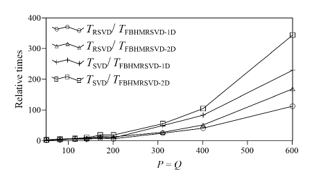
Figure 3. The comparative computational cost of obtaining a rank $r=10$ approximation for matrices of increasing size using Algorithm 3 with $q=1$ both with and without use of fast matrix-matrix multiplication, FBHMRSVD, and RSVD, respectively, and compared with the direct use of the SVD. Each experiment is performed $20$ times and the ratios are reported for the median result in each case.

3. Fast non-convex low-rank matrix decomposition potential field separation: FNCLRMD_PFS

3.1. Methodology

We suppose that the total field data matrix of size $P\times Q$ is

$$\mathbf{X}=\mathbf{X}_{D}+\mathbf{X}_{S},$$

where the gridded data matrices of the regional and residual anomalies are denoted by $\mathbf{X}_{D}$ and $\mathbf{X}_{S}$, respectively. Practically, $\mathbf{X}_{D}$ and $\mathbf{X}_{S}$ are unknown and the objective of potential field data separation is their estimation given $\mathbf{X}$. This means that the block Hankel matrix $\mathbf{T}=\mathcal{H}(\mathbf{X})$ represents $\mathbf{X}_{D}$ and $\mathbf{X}_{S}$, separately,

$$\mathbf{T}=\mathbf{T}_{D}+\mathbf{T}_{S}=\mathcal{H}(\mathbf{X}_{D})+\mathcal{H}(\mathbf{X}_{S}).$$

Because $\mathbf{T}_{D}$ is assumed to have low rank and $\mathbf{T}_{S}$ is assumed to be sparse, for which the derivations are given in [29], the separation can be achieved by solving the optimization problem

(4) $$\min\>\{\mathtt{rank}(\mathbf{T}_{D}),\|\mathbf{T}_{S}\|_{0}\}\quad\mathtt{subject\>to}\>\mathbf{T}=\mathbf{T}_{D}+\mathbf{T}_{S}.$$

The algorithm LRMD_PFS introduced in [29] uses a convex method to solve the optimization problem in (4) by transforming to the optimization problem,

(5) $$\min\>\|(\mathbf{T}_{D})\|_{*}+\alpha\|\mathbf{T}_{S}\|_{1},\>\>\>\mathtt{subject\>to}\>\mathbf{T}=\mathbf{T}_{D}+\mathbf{T}_{S},$$

where $\alpha>0$ denotes a weighting parameter. Because $\mathbf{T}$ is generally large, the solution of (5) is computationally demanding in terms of flops and memory. The Altproj Algorithm [17] to solve (4) is, however, non-convex and proceeds by alternately updating $\mathbf{T}_{S}$ by projecting $\mathbf{T}-\mathbf{T}_{D}$ onto the set of sparse matrices, and $\mathbf{T}_{D}$ by projecting $\mathbf{T}-\mathbf{T}_{S}$ onto the set of low-rank matrices. At each step the partial SVD of $\mathbf{T}$ is required. Thus, it is ideal to implement the Altproj Algorithm using the FBHMRSVD Algorithm 3 for all estimates of the partial SVD. The solution of (4) with the application of the Altproj Algorithm combined with Algorithm 3 is detailed in Algorithm 4, and is denoted by

$$[\mathbf{X}_{D}^{*},\mathbf{X}_{S}^{*}]=\mathtt{FNCLRMD\_PFS}(\mathbf{X},K,\hat{K},r^{*},\beta,M,\epsilon).$$

Here $r^{*}$, $\beta$, $M$, and $\epsilon$ are desired rank, thresholding parameter, an iteration parameter, and a convergence tolerance respectively.

Algorithm 4 Fast non-convex low-rank matrix decomposition potential field separation:
$[\mathbf{X}_{D}^{*},\mathbf{X}_{S}^{*}]=\mathtt{FNCLRMD\_PFS}(\mathbf{X},K,\hat{K},r^{*},\beta,M,\epsilon).$

1:  Input: potential field data matrix $\mathbf{X}\in\mathcal{R}^{P\times Q}$; parameter $K$ and $\hat{K}$; desired rank $r^{*}$; thresholding parameter $\beta$; iteration parameter $M$; convergence tolerance $\epsilon$.

2:  Definition: $\sigma_{j}(\mathbf{M})$ denotes the $j$th largest singular value of $\mathbf{M}$; $\mathtt{P}_{k}(\mathbf{H})$ denotes the best rank $k$ approximation of $\mathbf{H}$; $\mathtt{HT}_{\zeta}(\mathbf{H})$ denotes hard-thresholding applied to $\mathbf{H}$ such that entries with absolute values less than $\zeta$ are set to $0$; $\mathtt{IP}(\mathbf{H})$ denotes inverse projection for recovering the matrix from its trajectory matrix by averaging the counter diagonal of each one of its blocks [8].

3:  $[\mathbf{U}^{(0)},\mathbf{\Sigma}^{(0)},\mathbf{V}^{(0)}]=\mathtt{FBHMRSVD}(\mathbf{X},K,\hat{K},1,1,1)$,

4:  $\zeta_{0}=\beta\mathbf{\Sigma}^{(0)}(1,1)$.

5:  $\mathbf{X}_{D}^{(0)}=0$; $\mathbf{X}_{S}^{(0)}=\mathtt{HT}_{\zeta_{0}}(\mathbf{X}-\mathbf{X}_{D})$.

6:  for $k=1$ to $r^{*}$ do

7:     for $t=0$ to $M$ do

8:        $[\mathbf{U}^{(t+1)},\mathbf{\Sigma}^{(t+1)},\mathbf{V}^{(t+1)}]=\mathtt{FBHMRSVD}(\mathbf{X}-\mathbf{X}_{D}^{(t)},K,\hat{K},k+1,k+1,1)$.

9:        $\zeta=\beta(\mathbf{\Sigma}^{(t+1)}(k+1,k+1)+(\frac{1}{2})^{t}\mathbf{\Sigma}^{(t+1)}(k,k))$.

10:        $\mathbf{X}_{D}^{(t+1)}=\mathtt{IP}(\mathtt{P}_{k}(\mathbf{X}-\mathbf{X}_{D}^{(t)}))$, where $\mathtt{P}_{k}(\mathbf{X}-\mathbf{X}_{D}^{(t)})=\mathbf{U}_{k}^{(t+1)}\mathbf{\Sigma}_{k}^{(t+1)}(\mathbf{V}_{k}^{(t+1)})^{T}$.

11:        $\mathbf{X}_{S}^{(t+1)}=\mathtt{HT}_{\zeta}(\mathbf{X}-\mathbf{X}_{D}^{(T+1)})$.

12:        if $\lVert\mathbf{X}_{D}^{(t+1)}-\mathbf{X}_{D}^{(t)}\rVert_{2}<\epsilon$ then

13:           break

14:        else

15:           $\mathbf{X}_{S}^{(0)}=\mathbf{X}_{S}^{(t)}$.

16:        end if

17:     end for

18:  end for

19:  $\mathbf{X}_{D}^{*}=\mathbf{X}_{D}^{(t)}$, $\mathbf{X}_{S}^{*}=\mathbf{X}-\mathbf{X}_{D}^{*}$.

20:  Output: $\mathbf{X}_{D}^{*}$, $\mathbf{X}_{S}^{*}$.

3.2. Parameter setting

The quality of the solution of (4) in terms of separating the regional and residual anomalies depends on the parameters $r^{*}$ and $\beta$. The default interval for the adjustment of $\beta$, $0<\beta<1/\sqrt{\mathtt{max}(KL,\hat{K}\hat{L})}$ was recommended in [29]. Within this interval, experiments demonstrate that the results are consistent for a large subinterval. We will, see, however, that the quality of the separation is not very sensitive to the choice of $\beta$ and that the choice of $r^{*}$ is more significant. This is illustrated for synthetic geologic models for which the total field, regional anomaly, and residual anomaly are shown in Figures 4, 4, 5, and 5, respectively. The parameters of these models, for which the matrices are of sizes $201\times 201$, are detailed in Table 3. Figure 6 shows the RMSE when applying Algorithm 4 with $r^{*}=6$ and $10$ and different choices for $\beta$. While the RMSEs are relatively insensitive to $\beta\in[0.0003,0.007]$, it is evident from Figure 6, that the computational cost depends dramatically on the choice of $r^{*}$. This means the computational time is affected by $r^{*}$, but not $\beta$, and hence Algorithm 4 is relatively robust to the choice of $\beta$.

Now using $\beta\in[0.0003,0.007]$ as indicated from the previous experiment, the total field is separated for $r^{*}$ increasing from $1$ to $20$. The RMSEs of the results are shown in Figure 6 and it is immediate that the RMSE decreases rapidly for $r^{*}=1:4$, but is relatively stable and independent of $r^{*}$ for $r^{*}>4$. On the other hand, it is clear from Figure 6, that the computational cost increases with increasing $r^{*}$. Thus there is a trade-off in terms of accuracy and computational cost in how $r^{*}$ is chosen. Practically, however, due to the low-rank features of the regional anomaly, it is sufficient to take $r^{*}$ to be small, and generally not significantly larger than $10$.

Suitable separation of the anomalies is obtained using small values of the parameters $M$ and $\epsilon$. For all experiments reported here we use $M=10$ and $\epsilon=0$. Increasing $\epsilon$ to a small tolerance such as $10^{-3}$ or $10^{-7}$ will reduce the computational cost because the iteration will converge more quickly. Even with the chosen values, however, FNCLRMD_PFS is still much more efficient than LRMD_PFS.

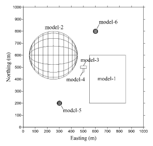
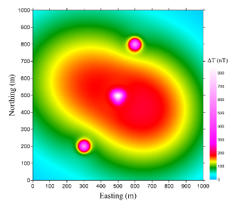
Figure 4. Figures 4 and 4 are the geologic models and the forward magnetic field, respectively.

Table 3. The parameters that define the geologic models in Figures 4 and 7.

Geologic model	Shape	Central position	Model parameters	Density	Magnetization
			(length, width, depth extent)/radius	(g/cm3)	(A/m)
model-$1$	Block	$(700,400,600)$	$(300,400,200)$	$0.5$	$8000$
model-$2$	sphere	$(250,600,700)$	$200$	$0.4$	$7000$
model-$3$	Block	$(500,500,40)$	$(50,20,40)$	$0.5$	$5000$
model-$4$	Block	$(500,475,40)$	$(10,30,40)$	$0.5$	$5000$
model-$5$	sphere	$(300,200,40)$	$20$		$5000$
model-$6$	sphere	$(600,800,40)$	$20$		$5000$
model-$7$	sphere	$(200,200,40)$	$20$	$0.7$
model-$8$	Block	$(800,800,40)$	$(80,80,40)$	$0.5$

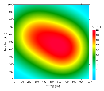
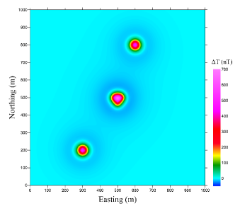
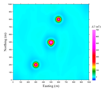
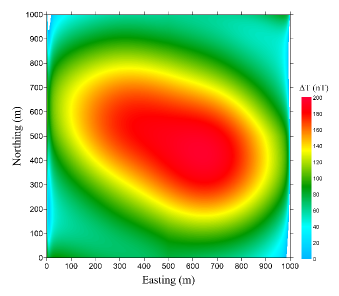
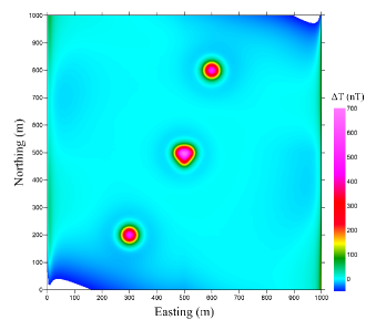
Figure 5. Figures 5 and 5 are the synthetic regional and residual anomalies for the models in Figure 4, respectively; Figures 5 and 5 are the separated regional and residual anomalies, respectively, for data of size $201\times 201$ obtained using Algorithm 4 with $\beta=0.0062$ and $r^{*}=6$; Figures 5 and 5 are the separated regional and residual anomalies, respectively, obtained using LRMD_PFS with $\alpha=0.0005$.

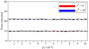
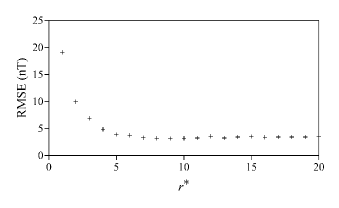
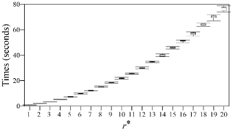
Figure 6. These results show tests of the parameters for Algorithm 4. Figures 6 and 6 are the RMSE and the computational times for the separations of the data in Figure 4 with different $\beta$; Figures 6 and 6 are the RMSE and the computational times of the separations of the data in Figure 4 with different $r^{*}$.

4. SYNTHETIC FIELD DATA EXPERIMENTS

4.1. Experiment 1: Magnetic Data

The accuracy and the computational cost of Algorithm 4, dependent on $\beta$, for the gridded data matrices in Figure 4, for matrices of different sizes, is contrasted with the results obtained using LRMD_PFS dependent on $\alpha$. The experiment is repeated for different choices of $\beta$ and $\alpha$ in the recommended intervals, and the result with the smallest RMSE is selected as the final result and reported in Table 4, with illustration in Figures 5-6. The RMSEs obtained using Algorithm 4 are between $3.53$ and $3.78$ nT, while the RMSEs for the same experiments using LRMD_PFS are between $13.80$ and $16.39$ nT, hence demonstrating the higher accuracy of the new algorithm. It is more significant, however, that Algorithm 4 performs better than LRMD_PFS with respect to computational cost in terms of computational time and memory demand. Moreover, in the given computational environment, it is not possible to obtain the data matrices of sizes much greater than $205\times 205$ using LRMD_PFS. In contrast, it is possible to solve the problem for matrices of sizes $2001\times 2001$ using Algorithm 4. For the smaller problem of size $201\times 201$, Figures 5 and 5 show the separated regional and residual anomalies using Algorithm 4, while Figures 5 and 5 show the separated anomalies obtained using LRMD_PFS. It can be seen from Figures 5 to 5, that Algorithm 4 performs well around the boundaries, but that the two methods are comparable in the central areas.

Table 4. Comparisons of the computational times of the FBHMRSVD, RSVD, and SVD. $/$ denotes that either the computational time is too high to perform the experiment, or an “out of memory” error is reported.

Matrix sizes		FNCLRMD_PFS				LRMD_PFS
$\mathbf{X}$	$\mathbf{T}$	$r^{*}$	$\beta$	RMSE (nT)	Times (s)	$\alpha$	RMSE (nT)	Times (s)
$141\times 141$	$5041\times 5041$	$6$	$0.013$	$3.53$	$4.93$	$0.001$	$15.10$	$128.28$
$171\times 171$	$7396\times 7396$	$6$	$0.0088$	$3.64$	$5.51$	$0.0008$	$14.46$	$446.20$
$201\times 201$	$10201\times 10201$	$6$	$0.0062$	$3.60$	$9.77$	$0.0005$	$13.80$	$1043.37$
$311\times 311$	$22801\times 22801$	$6$	$0.0026$	$3.61$	$23.94$	$/$	$/$	$/$
$401\times 401$	$40401\times 40401$	$6$	$0.0014$	$3.65$	$40.42$	$/$	$/$	$/$
$601\times 601$	$90601\times 90601$	$6$	$0.0007$	$3.65$	$87.21$	$/$	$/$	$/$
$1001\times 1001$	$251001\times 251001$	$6$	$0.0002$	$3.75$	$218.54$	$/$	$/$	$/$
$2001\times 2001$	$1002001\times 1002001$	$6$	$0.00002$	$4.22$	$1062.29$	$/$	$/$	$/$

4.2. Experiment 2: Gravity Data

For this experiment, the synthetic geologic models, the total field, the regional anomaly and the residual gravity anomaly are shown in Figures 7, 7, 8, and 8, respectively. The parameters that define the models, all for data matrices of size $201\times 201$, are detailed in Table 3, and the results are illustrated in Figure 8. In contrast to Experiment 1 (in 4.1), the residual anomaly is generated for geologic models with different scales. In the application of Algorithm 4 for the separation of the data we set $r^{*}=6$ and $\beta=0.0005$. This yields a RMSE of $0.0028$ mGal. In contrast the smallest RMSE using LRMD_PFS is $0.017$ mGal and is obtained with $\alpha=0.0007$. Thus, Algorithm 4 yields a higher accuracy result. Moreover, the computational clock times are $46.47$ and $2249.69$ s, respectively. Hence, Algorithm 4 is much more efficient. The results of the separation by the two methods are shown in Figures 8 to 8. It can be seen from Figures 8 to 8, that the obtained gravity values of the separated regional anomaly in the north-east region using LRMD_PFS are higher than the synthetic regional anomaly. Thus, not only is Algorithm 4 more efficient, the results are qualitatively better.

In summary, our experiments demonstrate that Algorithm 4 has higher accuracy and lower computational cost than the LRMD_PFS for the separation of both magnetic and gravity data.

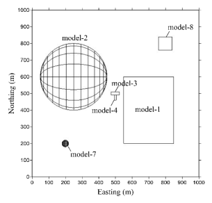
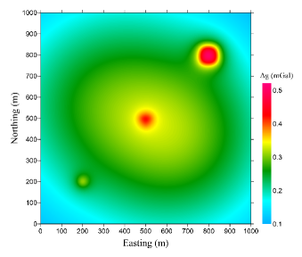
Figure 7. Figures 7 and 7 are the geologic models and the forward gravity field, respectively.

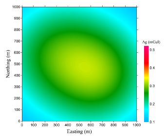
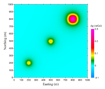
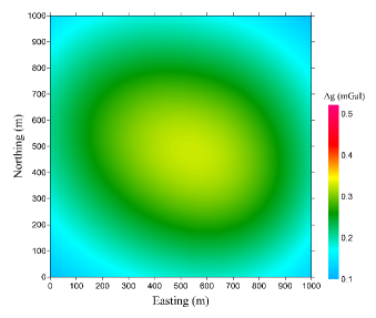
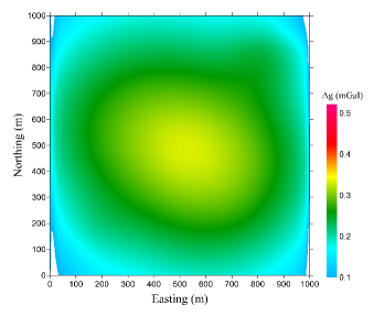
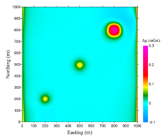
Figure 8. Figures 8 and 8 are the synthetic regional and residual anomalies for the models in Figure 7, respectively; Figures 8 and 8 are the separated regional and residual anomalies, respectively, for data of size $201\times 201$ obtained using Algorithm 4 with $\beta=0.0005$ and $r^{*}=6$; Figures 8 and 8 are the separated regional and residual anomalies, respectively, obtained using LRMD_PFS with $\alpha=0.0007$.

5. An Investigation of FNCLRMD_PFS for a practical data set

The Tongling region is a good example of skarn deposits lying in Anhui province of China. The Fenghuangshan copper deposit, which is a famous area in the Tongling region, is situated in the east central of the Middle-lower Yangtze metallogenic belt. The mineral deposits are generally of hydrothermal metasomatic type. Thus, the ore bodies occur in the contact zones between igneous rocks and sedimentary rocks. Therefore, in order to predict the location of concealed ore bodies, the separation of anomalies produced by igneous rocks is required.

The study area has three types of rocks. These include sedimentary rocks, igneous rocks, and skarn (or ore body). The physical properties of the sedimentary rocks are medium densities and non-magnetizations, while the igneous rocks are low density (with residual density $-0.1$ g/cm³) and medium magnetization (with magnetic susceptibility $0\thicksim 3400\times 10^{-6}\times 4\pi$ SI). In contrast, the skarn and ore bodies are of high density (with residual density $0.7$ g/cm³) and strong magnetization (with magnetic susceptibility larger than $10000\times 10^{-6}\times 4\pi$ SI). The difference in the density and magnetic properties of these different rocks makes it effective to study the igneous rocks and ore bodies through gravity and magnetic exploration. Our objective is to separate the combination of regional anomalies of low-gravity and high-magnetism that are produced by igneous rocks, and the combination of local anomalies of high-gravity and high-magnetism produced by skarn and ore bodies. Thus providing a basis for inversion and interpretation.

The algorithm is applied for the separation of the anomalies in Figure 9. Figure 9 is a Bouguer gravity anomaly map. The Bouguer gravity anomalies in the study area are high in the north (about $12$mGal) and low in the south (about $3$mGal). The data matrix has size $247\times 257$. In separating the gravity field we use $r^{*}=10$ and $\beta=0.01$, yielding the separated regional and residual gravity anomalies shown in Figures 10 and 10, respectively.

The reduce to the pole (RTP) magnetic anomaly is shown in Figure 9. There is a local high magnetic anomaly centered around Xinwuling. The size of the magnetic data matrix is $197\times 199$. In separating the RTP magnetic field we use $r^{*}=10$ and $\beta=0.005$, yielding the separated regional and residual magnetic anomalies shown in Figures 10 and 10, respectively.

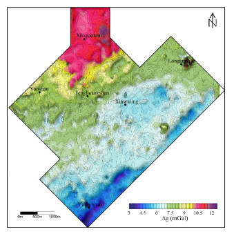
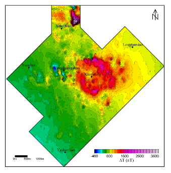
Figure 9. Figures 9 and 9 are the maps of the Bouguer gravity and the RTP magnetic anomalies of the study area in Tongling.

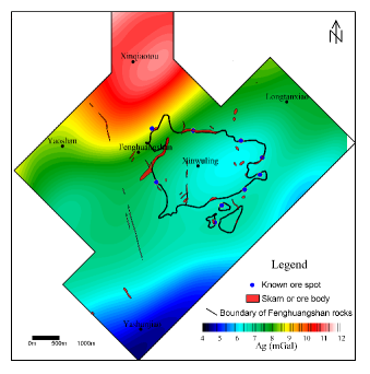
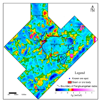
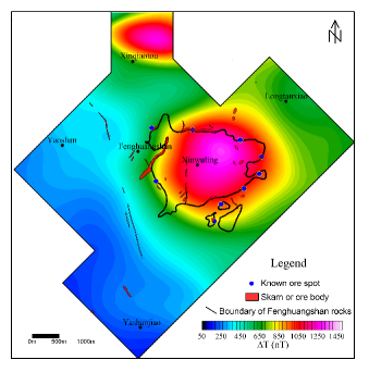
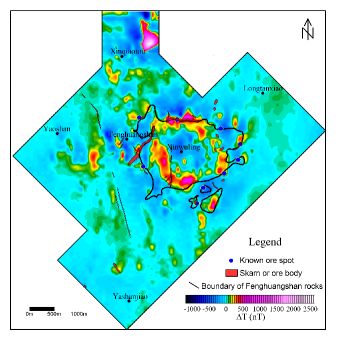
Figure 10. Figures 10 and 10 are the separated regional and residual gravity anomalies of the study area, respectively; Figures 10 and 10 are the separated regional and residual magnetic anomalies of the study area, respectively.

As we can see in Figure 10, the separated regional gravity anomaly reflects the structures of deep underground sources, and it also reflects the distribution of the igneous rocks in the deep for the corresponding local low gravity anomaly and known Fenghuangshan rocks. Due to the good correspondence of the high magnetic anomaly with Fenghuangshan rocks, the separated regional magnetic anomaly mainly reflects the distribution of the igneous rocks in the deep. The gravity anomaly low and magnetic anomaly highs extend to the north-east of the Fenghuangshan rocks. Thus, the Fenghuangshan rocks in the deep are deduced to extend to the north-east. The areas which correspond to local high gravity and magnetic anomalies in Figures 10 and 10 are inferred to be skarns or shallow ore bodies which is consistent with known ore and skarn located in these areas. Therefore, we infer the unknown areas which may exhibit mineralizations based on the relations of the gravity and magnetic anomalies in Figures 10 and 10, as shown in Figure 11.

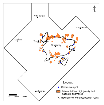
Figure 11. Predictions of the distributions of areas that may have sharns or ore bodies based on the separated high-gravity and high-magnetic fields.

6. Conclusions

A fast non-convex low-rank matrix decomposition algorithm, FNCLRMD_PFS, for the separation of potential field data has been presented and validated. The core of FNCLRMD_PFS is the efficient computation of the partial SVD of the block Hankel trajectory matrix, $\mathbf{T}$, without direct construction of $\mathbf{T}$. Thus, the low-rank matrix decomposition non-convex algorithm for potential field data separation can be realized without requiring the storage of construction $\mathbf{T}$, and the resulting storage and computational costs are lower than required when using LRMD_PFS. FNCLRMD_PFS depends on two parameters, these are the estimate $r^{*}$ of the rank of the regional anomaly matrix, and a threshold parameter $\beta$. Synthetic experiments were used to obtain recommendations for the settings of these parameters. These show that a suitable default interval for adjusting $\beta$ is $0<\beta<1/\sqrt{\mathtt{max}(KL,\hat{K}\hat{L})}$. The parameter $r^{*}$, when it is not too small, mainly influences the computational time but not the accuracy. The experimental results demonstrate that the presented algorithm is robust and, thus, the choice of parameters, provided the interval for $\beta$ and rank $r^{*}$ are chosen as recommended, is straightforward.

Synthetic data sets were set up for gravity and magnetic data and used to contrast the accuracy and computational cost of FNCLRMD_PFS with LRMD_PFS. These results demonstrated that FNCLRMD_PFS has higher accuracy and is more computationally efficient than LRMD_PFS. Moreover, it is feasible to use FNCLRMD_PFS for matrices of much larger size than is possible with LRMD_PFS which exhibits either with an extreme requirement on computational time or the report of “out of memory” for matrices of large size. Specifically, FNCLRMD_PFS can be used to compute large size potential field data with high accuracy at acceptable computational cost. Finally, FNCLRMD_PFS was also used for the separation of real data in the Tongling area, Anhui province, China. The separated low-gravity and high-magnetic regional anomalies have good correspondence to the igneous rocks, and the separated high-gravity and high-magnetic residual anomalies exhibit good correspondence to the known ore spots. Consequently, unknown areas of mineralizations can be inferred from the separated anomalies.

Appendix A Notation

Acronyms and notation used throughout are provided in Tables 5 and 6.

Table 5. Acronyms used throughout

Acronym	Description
FBHMRSVD	fast block Hankel matrix randomized SVD algorithm
FBHMMM	fast block Hankel matrix-matrix multiplication algorithm
FBHMVM	fast block Hankel matrix-vector multiplication Algorithm
FNCLRMD_PFS	fast non-convex low-rank matrix decomposition algorithm for potential field separation
EALM	exact augmented Lagrange multiplier method
IALM	inexact augmented Lagrange multiplier method
LRMD_PFS	low-rank matrix decomposition for potential field separation
RPCA	robust principal component analysis
RSVD	randomized singular value decomposition
SVD	singular value decomposition
RMSE	root mean square error
RTP	reduce to the pole

Table 6. Notation used throughout

Notation	Description
$\mathbf{J}$	exchange matrix
$\mathbf{X}$	2D gridded potential field data matrix
$\mathbf{T}_{j}$	Hankel matrix constructed from the $j$th column of $\mathbf{X}$
$\mathbf{T}$	trajectory matrix of $\mathbf{X}$
$\mathbf{X}_{1},\cdots,\mathbf{X}_{Q}$	first to $Q$th columns of $\mathbf{X}$, respectively
$\mathbf{U},\mathbf{V},\mathbf{\Sigma}$	SVD of $\mathbf{T}$, $\mathbf{T}=\mathbf{U}\mathbf{\Sigma}V^{T}$
$\mathbf{U}_{r},\mathbf{V}_{r},\mathbf{\Sigma}_{r}$	rank-$r$ partial SVD of $\mathbf{T}$ using FBHMRSVD
$\mathbf{X}_{D}$, $\mathbf{X}_{S}$	data matrices of regional and residual anomalies, respectively
$\mathbf{T}_{D}$, $\mathbf{T}_{S}$	trajectory matrices of $\mathbf{X}_{D}$ and $\mathbf{X}_{S}$, respectively
$\mathbf{X}_{D}^{*}$, $\mathbf{X}_{S}^{*}$	approximations of $\mathbf{X}_{D}$ and $\mathbf{X}_{S}$ using FNCLRMD_PFS, respectively
$\mathbf{u}_{1},\mathbf{u}_{2},\cdots$	$\mathbf{U}=[\mathbf{u}_{1},\mathbf{u}_{2},\cdots]$, $\mathbf{u}_{1},\mathbf{u}_{2},\cdots$ are the left singular vectors of $\mathbf{T}$
$\mathbf{v}_{1},\mathbf{v}_{2},\cdots$	$\mathbf{V}=[\mathbf{v}_{1},\mathbf{v}_{2},\cdots]$, $\mathbf{v}_{1},\mathbf{v}_{2},\cdots$ are the right singular vectors of $\mathbf{T}$
$x_{mn}$	element at $m$th row and $n$th column of $\mathbf{X}$
$P$, $Q$	$\mathbf{X}$ is of size $P\times Q$
$K$, $L$	$\mathbf{T}_{j}$ is of size $K\times L$
$\hat{K}$, $\hat{L}$	$\mathbf{T}$ is a block Hankel matrix with $\hat{K}\times\hat{L}$ blocks
$P_{C}$, $Q_{C}$	$\mathbf{C}$ is of size $P_{C}\times Q_{C}$
$\sigma_{1}$, $\sigma_{2}$, $\cdots$	$\mathbf{\Sigma}=\mathtt{diag}(\sigma_{1}^{2},\sigma_{2}^{2},\cdots)$, where $\sigma_{1}$, $\sigma_{2}$ , $\cdots$ are the singular values of $\mathbf{T}$
$r$	desired rank parameter in FBHMRSVD
$p$	oversampling parameter in FBHMRSVD
$q$	power iteration parameter in FBHMRSVD
$r^{*}$	desired rank parameter in FNCLRMD_PFS
$\beta$	thresholding parameter in FNCLRMD_PFS
$\alpha$	weighting parameter in LRMD_PFS
$\|\cdot\|_{p}$, $\|\cdot\|_{*}$	$\ell_{p}$ and nuclear norms, respectively
$T_{\mathtt{SVD}}$	computational cost of SVD
$T_{\mathtt{RSVD}}$	computational cost of RSVD
$T_{\mathtt{FBHMRSVD}}$	computational cost of FBHMRSVD

Appendix B The impact of the choice of the FFT used by MATLAB on the computational cost

Our initial investigation of the computational cost of Algorithm 1 demonstrated a general tendency for the computational cost to increase monotonically with increasing size of the matrices. There were, however, outlier sizes which were significantly higher in cost and departed from the general monotonic increase in time. This is illustrated in Figure 12 for which we conducted an experiment to test the cost of step 1 in Algorithm 1 using the $\mathtt{vec}(\mathbf{X})$ with its dimensions between $2^{15}$ and $80000$. For each matrix dimension, the code is run $80$ times, and the average time is calculated. But, because the MATLAB function determines an optimal transform to use for a given matrix size, at greater cost in the first run, this first run is excluded from the estimate of the average cost for each matrix size. A spike in cost is seen between $60000$ and $70000$, actually at $63001$, but overall the tendency is a gradual increase in computational cost and outliers are not frequent. We note that $63001=251\times 251$ is not prime but $251$ is prime, and the determination of an optimal transform depends on the factorization of the transform size. We conclude that there may be cases where the computational cost of Algorithm 1 spikes because of this situation. On the other hand, for the problem of this size the calculation of the RSVD with, and without, the use of Algorithm 2 for the matrix multiplications has a computational cost in each case of $2.614$ s and $30.885$ s, respectively. Hence, even when the FFT transform is relatively slow, the use of a fast block Hankel matrix multiplication is still faster than the use of a direct matrix-multiplication without the use of the FFT.

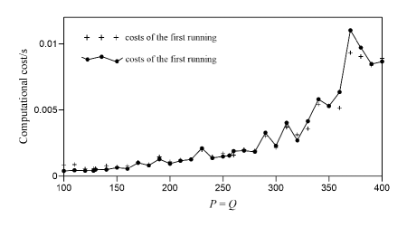
Figure 12. Demonstrating non-monotonic increase in computational time using Algorithm 1 for $P\times Q$ between $2^{15}$ and $80000$.

References

- [1] W. B. Agocs, Least squares residual anomaly determination, Geophysics, 16 (1951), 686–696.
- [2] A. Beck and M. Teboulle, A fast iterative shrinkage-thresholding algorithm for linear inverse problems, SIAM Journal on Imaging Sciences, 2 (2009), 183–202.
- [3] D. S. Broomhead and G. P. King, Extracting qualitative dynamics from experimental data, Physica D: Nonlinear Phenomena, 20 (1986), 217–236.
- [4] E. J. Candès, X. D. Li, Y. Ma and J. Wright, Robust principal component analysis?, Journal of the ACM (JACM), 58 (2011), 11.
- [5] K. C. Clarke, Optimum second-derivative and downward-continiation filters, Geophysics, 34 (1969), 424–437.
- [6] M. Fedi and T. Quarta, Wavelet analysis for the regional-residual and local separation of potential field anomalies, Geophysical Prospecting, 46 (1998), 507–525.
- [7] G. H. Golub and C. F. Van Loan, Matrix computations, Johns Hopkins Press, Baltimore, 1996.
- [8] N. Golyandina, I. Florinsky, and K. Usevich, Filtering of digital terrain models by 2D singular spectrum analysis, International Journal of Ecology & Development, 8 (2007), 81–94.
- [9] Z. Z. Hou and W. C. Yang, Wavelet transform and multi-scale analysis on gravity anomalies of China, Chinese Journal of Geophysics, 40 (1997), 85–95.
- [10] N. Halko, P. Martinsson, and J. A. Tropp, Finding structure with randomness: probabilistic algorithms for constructing approximate matrix decompositions, SIAM Review, 53 (2011), 217–288.
- [11] E. Liberty, F. Woolfe, P. Martinsson, V. Rokhlin and M. Tygert, Randomized algorithms for the low-rank approximation of matrices, Proceedings of the National Academy of Sciences, 104 (2007), 20167–20172.
- [12] Z. C. Lin, M. M. Chen, and Y. Ma, The augmented Lagrange multiplier method for exact recovery of corrupted low-rank matrices, preprint, arxiv: https://arxiv.org/abs/1009.5055.
- [13] Z. C. Lin and H. Y. Zhang, Low-rank models in visual analysis, Elsevier Science Publishing Co Inc, New York, 2017.
- [14] L. Lu, W. Xu and S. Z. Qiao, A fast SVD for multilevel block Hankel matrices with minimal memory storage, Numerical Algorithms, 69 (2015), 875–891.
- [15] A. Mandal, and S. Niyogi, Filter assisted bi-dimensional empirical mode decomposition: a hybrid approach for regional-residual separation of gravity anomaly, Journal of Applied Geophysics, 159 (2018), 218–227.
- [16] K. L. Mickus, C. L. V. Aiken and W. D. Kennedy, Regional-residual gravity anomaly separation using the minimum-curvature technique, Geophysics, 56 (1991), 279–283.
- [17] P. Netrapalli, U. N. Niranjan, S. Sanghavi, A. Anandkumar, and P. Jain, Non-convex robust PCA, Advances in Neural Information Processing Systems, (2014), 1107–1115.
- [18] R. S. Pawlowski, Preferential continuation for potential-field anomaly enhancement, Geophysics, 60 (1995), 390–398.
- [19] R. S. Pawlowski and R. O. Hansen, Gravity anomaly separation by Wiener filtering, Geophysics, 55 (1990), 539–548.
- [20] A. Spector and F. S. Grant, Statistical models for interpreting aeromagnetic data, Geophysics, 35 (1970), 293–302.
- [21] F. Takens, Detecting strange attractors in turbulence, Dynamical systems and turbulence, Warwick 1980,(1981), 366–381.
- [22] W. M. Telford, L. P. Geldart and R. E. Sheriff, Applied geophysics, Cambridge University Press, Cambridge, 2003.
- [23] A. A. Tsonis and J. B. Elsner, Mapping the channels of communication between the tropics and higher latitudes in the atmosphere, Physica D: Nonlinear Phenomena, 92 (1996), 237–244.
- [24] S. Vatankhah, R. A. Renaut and V. E. Ardestani, A fast algorithm for regularized focused 3D inversion of gravity data using randomized singular-value decomposition, Geophysics, 83 (2018), G25–G34.
- [25] C. R. Vogel, Computational Methods for Inverse Problems, Society for Industrial and Applied Mathematics, Philadelphia, 2002.
- [26] J. Wright, Y. Ma, J. Mairal, G. Sapiro, T. Huang and S. C. Yan, Sparse representation for computer vision and pattern recognition, Proceedings of the IEEE, 98 (2010), 1031–1044.
- [27] W. C. Yang, Z. Q. Shi, Z. Z. Hou and Z. Y. Cheng, Discrete wavelet transform for multiple decomposition of gravity anomalies, Chinese Journal of Geophysics, 44 (2001), 534–541.
- [28] L. L. Zhang, T. Y. Hao and W. W. Jiang, Separation of potential field data using 3-D principal component analysis and textural analysis, Geophysical Journal International, 179 (2009), 1397–1413.
- [29] D. Zhu, H. W. Li, T. Y. Liu, L. H. Fu, S. H. Zhang, Low-rank matrix decomposition method for potential field data separation, Geophysics, 85 (2020), G1–G16.