Transport of Spin and Mass at Normal-Superfluid Interfaces
in the Unitary Fermi Gas

Abstract

Transport in strongly interacting Fermi gases provides a window into the non-equilibrium behavior of strongly correlated fermions. In particular, the interface between a strongly polarized normal gas and a weakly polarized superfluid at finite temperature presents a model for understanding transport at normal-superfluid and normal-superconductor interfaces. An excess of polarization in the normal phase or a deficit of polarization in the superfluid brings the system out of equilibrium, leading to transport currents across the interface. We implement a phenomenological mean-field model of the unitary Fermi gas, and investigate the transport of spin and mass under non-equilibrium conditions. We consider independently prepared normal and superfluid regions brought into contact, and calculate the instantaneous spin and mass currents across the normal-superfluid (NS) interface. For an unpolarized superfluid, we find that spin current is suppressed below a threshold value in the driving chemical potential differences, while the threshold nearly vanishes for a critically polarized superfluid. The mass current can exhibit a threshold in cases where Andreev reflection vanishes, while in general Andreev reflection prevents the occurrence of a threshold in the mass current. Our results provide guidance to future experiments aiming to characterize spin and mass transport across NS interfaces.

I Introduction

Experiments on quantum gases of atoms enable strong tests of many-body theories. Studies of ultracold Fermi gases have provided insight into the thermodynamics, excitation spectra, and bulk transport properties of strongly interacting fermions, e.g. Shin et al. (2008); Navon et al. (2010); Nascimbène et al. (2010, 2011); Ku et al. (2012); Van Houcke et al. (2012); Schirotzek et al. (2008); Gaebler et al. (2010); Hoinka et al. (2017); Sommer et al. (2011a, b); Cao et al. (2011); Enss and Haussmann (2012); Valtolina et al. (2017); Enss and Thywissen (2019); Tajima et al. (2020). Measurements of fermion transport through quantum point contacts Brantut et al. (2012); Husmann et al. (2015); Krinner et al. (2016); Kanász-Nagy et al. (2016); Häusler et al. (2017); Corman et al. (2019); Ono et al. (2021) and Josephson junctions Valtolina et al. (2015); Burchianti et al. (2018); Zaccanti and Zwerger (2019); Luick et al. (2020); Del Pace et al. (2021) have extended atomic Fermi gas experiments into the domain of structured devices. Meanwhile, strongly correlated electron materials such as high-temperature superconductors have gained growing interest for application in devices, such as Josephson junctions Berggren et al. (2016); Perconte et al. (2018), spin valves Visani et al. (2012); Komori et al. (2018), and semiconductor-superconductor junction devices Bouscher et al. (2020), that feature normal-superconductor interfaces. Experiments on cold atom-based systems that emulate normal-superconductor junctions can therefore provide valuable insight into the effects of strong correlations on transport in such devices. More fundamentally, atomic gas experiments provide a platform for controlled studies of strongly interacting systems out of equilibrium, and can therefore aid in the development of theoretical techniques for understanding the dynamics of many-body systems.

Spin-imbalanced unitary Fermi gases provide a natural model system in which to study strongly correlated normal-superfluid junctions. At low temperatures, when the difference in chemical potential between the two spin components exceeds the Chandrasekhar-Clogston limit, the system phase separates into a weakly polarized superfluid and a strongly polarized normal fluid that coexist at equilibrium Bulgac and Forbes (2007); Shin et al. (2008); Shin (2008); Baur et al. (2009); Nascimbène et al. (2010); Pilati and Giorgini (2008); Liu et al. (2008); Olsen et al. (2015). Spin-imbalanced Fermi gases therefore naturally form a normal-superfluid (NS) interface akin to the ferromagnet-superconductor interfaces employed in superconducting spin valves de Jong and Beenakker (1995); Halterman and Valls (2004); Kashimura et al. (2010); Alidoust and Halterman (2018). Transport across NS interfaces results from non-equilibrium conditions, making strongly interacting Fermi gases an interesting model of non-equilibrium behavior in strongly correlated systems.

Several previous works have considered aspects of transport across NS interfaces in strongly interacting Fermi gases. Calculations of thermal conductivity across the NS interface predicted a suppression of thermal conduction across the interface in chemical equilibrium Van Schaeybroeck and Lazarides (2007, 2009). Analysis of evaporation dynamics in trapped spin-imbalanced gases predicted a modification of the apparent critical polarization due to non-equilibrium spin distribution  Parish and Huse (2009). Experiments on spin-imbalanced Fermi gases observed metastability of non-equilibrium NS interfaces, which the authors attributed partly to inhibition of spin transport at the interface Liao et al. (2011). Measurements of spin transport coefficients found strong damping of the spin dipole mode in spin-balanced Sommer et al. (2011a) and spin-imbalanced gases with and without a superfluid core Sommer et al. (2011b), and experiments on fermionic quantum point contacts observed suppressed spin conductance with decreasing temperature  Krinner et al. (2016). Numerical simulations have recently predicted metastable spin-polarized droplets in superfluid Fermi gases Magierski et al. (2019).

In this paper, we investigate theoretically the transport of spin and mass across the NS interface in the spin-imbalanced unitary Fermi gas. We address three main questions: how much spin and mass current flows across the interface under a given set of conditions? Under what conditions does the superfluid excitation gap significantly inhibit spin or mass transport? And to what extent does Andreev reflection cause the mass current to behave differently from the spin current? To address these questions, we consider the interface between normal and superfluid regions out of chemical equilibrium and calculate the instantaneous spin and mass currents by employing a phenomenological mean-field model. We consider two situations: first, the case of normal and superfluid regions separated by a tunneling barrier potential; and second, the case without a barrier, where the normal and superfluid regions are in mechanical equilibrium. Our calculations provide guidance to future experiments on non-equilibrium NS interfaces by establishing the expected magnitude and behavior of the transport currents.

Our results show that the spin current flowing into a superfluid is suppressed below a threshold in the driving chemical potential difference. The predicted threshold is analogous to the threshold in the current-voltage (I-V) curve of normal-superconductor junctions at large barrier strength Blonder et al. (1982), employed in scanning tunneling spectroscopy to measure superconducting gaps Fischer et al. (2007). In analogy with scanning tunneling spectroscopy, the threshold is related to the minimum in the superfluid excitation spectrum. We find that, for an unpolarized superfluid in contact with a highly polarized normal region, the threshold in chemical potential differences between normal and superfluid regions matches the superfluid gap parameter (Section IV), up to a temperature-dependent correction that we identify in Section IV B. For a critically polarized superfluid (at finite temperature), the minimum in the superfluid excitation spectrum is significantly reduced, leading to a significant reduction in the threshold for transport current. The existence of a threshold supports the notion that non-equilibrium NS interfaces can persist in a metastable configuration. The transport threshold applies specifically to the non-Andreev portion of the current and therefore always affects the spin current. On the other hand, the net (mass) current can have a significant Andreev component, and therefore does not always exhibit a threshold.

The remainder of the paper is structured as follows. In Section II we introduce our phenomenological mean-field model, and in Section III we outline the calculation of the transport currents. In Section IV we present and discuss our results, and we conclude in Section V.

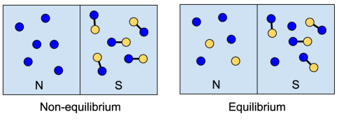
Figure 1: Schematic of non-equilibrium and equilibrium states of a phase-separated spin-imbalanced Fermi gas at finite temperature. Blue: majority (spin up), yellow: minority (spin down); lines represent Cooper pairing.

II Theoretical Model

II.1 Description of the Problem

We consider a unitary Fermi gas confined in a three-dimensional box potential Mukherjee et al. (2017) at low temperature, divided into left and right regions. The confining potential has a uniform cross section perpendicular to the $z$ axis. In the left region ($z<0$), the gas has a large spin polarization and is in the normal phase. In the right region ($z>0$), the gas has a smaller spin polarization and is in the superfluid phase. The densities of spin-up and spin-down fermions are uniform within a given region. The temperatures of the two regions can in general differ, but we will consider the case of equal temperatures for the two regions. Due to phase separation below the tricritical point Shin et al. (2008); Gubbels and Stoof (2008), the system can be in equilibrium or out of equilibrium, depending on the degree of polarization in each region. Figure 1 illustrates qualitatively the equilibrium and non-equilibrium configurations of the system under consideration. We will focus on calculating the instantaneous currents of spin-up and spin-down fermions across the interface between the two regions.

Figure 2 shows the approximate phase diagram of the spin-imbalanced homogeneous unitary Fermi gas. The polarization $p=(n_{\uparrow}-n_{\downarrow})/(n_{\uparrow}+n_{\downarrow})$ characterizes the degree of spin imbalance, where $n_{\sigma}$ gives the number density of fermions with spin projection $\sigma$. The phase diagram of Fig. 2 focuses on the case of a spin-up majority ($p>0$) and normalizes the temperature by the majority Fermi temperature $T_{F\uparrow}=E_{F\uparrow}/k_{B}$. Here $k_{B}$ is the Boltzmann constant and $E_{F\uparrow}=\hbar^{2}(6\pi^{2}n_{\uparrow})^{2/3}/(2m)$, where $m$ is the mass of the fermions. As in Ref. Shin et al. (2008), we approximate the phase boundaries as straight lines in the $p-T$ plane. In the non-equilibrium two-region configuration that we consider, each region is internally described by a point $(p_{i},T)$ on the equilibrium phase diagram, with the same absolute temperature $T$. The two regions have differing polarization, with the left (normal) side having polarization $p_{N}$ and the right (superfluid) side having polarization $p_{S}$.

For a given $T/T_{F\uparrow}$, the superfluid phase has a maximum (critical) polarization of $p_{Sc}$, while the normal phase has a minimum (critical) polarization of $p_{Nc}$. Below the tricritical temperature $T_{c3}$, the normal-to-superfluid phase transition is first-order, and the polarization is discontinuous, with $p_{Sc}<p_{Nc}$. At equilibrium, a system with global polarization $(N_{\uparrow}-N_{\downarrow})/(N_{\uparrow}+N_{\downarrow})$ between $p_{Sc}$ and $p_{Nc}$ will exhibit phase separation into a superfluid region and a normal region (here $N_{\uparrow}$ and $N_{\downarrow}$ are the total number of spin up and spin down fermions in a homogeneous box potential). At equilibrium, the phase-separated regions attain their critical polarizations, $p_{S}=p_{Sc}$ and $p_{N}=p_{Nc}$, respectively.

Our analysis will focus on the temperature regime below the tricritical point. For context, we will briefly review a few other features of the phase diagram. Above the tricritical temperature, the phase transition is second order and the polarization is continuous ($p_{Sc}=p_{Nc}$). The superfluid region of the phase diagram above the tricritical point is predicted to feature further subdivision into a gapped superfluid and a gapless Sarma superfluid Gubbels and Stoof (2008, 2013). For our analysis, we focus on temperatures below the tricritical temperature, and therefore do not consider the Sarma phase. We do not consider the Fulde-Ferrell-Larkin-Ovchinnikov (FFLO) phase Sheehy and Radzihovsky (2006); Son and Stephanov (2006); Yoshida and Yip (2007); Parish et al. (2007); Jensen et al. (2007); Kinnunen et al. (2018), which is predicted to occur away from unitarity in the regime of negative scattering length Sheehy and Radzihovsky (2006); Yoshida and Yip (2007); Parish et al. (2007), because we focus on the case of unitary (resonant) interactions. An interesting p-wave superfluid phase has been predicted in highly spin-imbalanced Fermi gases Bulgac et al. (2006); Bulgac and Yoon (2009). Theoretical calculations predict that the p-wave phase should occur at low temperatures over a range of polarizations above a polarization of about 0.8 in the unitary Fermi gas Patton and Sheehy (2012). For simplicity, we do not include the p-wave phase in our analysis, as it covers a relatively small portion of the phase diagram. However, it would be interesting to consider transport in the p-wave phase in future work.

In addition to the confining potential, we allow for a thin barrier potential in the $z=0$ plane separating the two regions. We model the barrier as a Dirac delta function, $V(z)=\Lambda\delta(z)$. For convenience, we parameterize the barrier strength as

$$k_{\Lambda}=2m\Lambda/\hbar^{2}$$ (1)

Experimentally, such a barrier would assist in the preparation of the non-equilibrium condition that we consider here, by allowing the two regions to equilibrate separately before initiating transport, similar to Refs. Valtolina et al. (2017); Krinner et al. (2016). The barrier strength can then be reduced, or turned to zero, to allow currents to flow as the system begins to evolve toward global equilibrium. The temperatures of two independently prepared regions will not in general be equal, but nearly equal temperatures can be achieved through fine tuning of the cooling process applied to each region during preparation. During transport measurements, maintaining a non-zero barrier may be helpful in controlling the magnitudes of the currents. We will consider particular cases of both zero and non-zero barrier strengths.

Our analysis will focus on the instantaneous currents under a given set of conditions. Over a finite time, one would need to consider additional dynamics. For example, the flow of particles across the interface will generate entropy and heat the system Chaikin and Lubensky (1995). The final temperature could exceed the tricritical temperature, in which case phase separation would not be present in the final state. The final equilibrium state will depend on the volumes of the two initial regions, whereas the instantaneous currents that we calculate here depend only on the local properties of the two regions. Furthermore, as particles flow across the interface, the interface itself can move and will therefore not always be located at $z=0$. Under conditions in which the system heats above the tricritical temperature, the interface would not be thermodynamically stable, and could evolve away from a planar geometry, in analogy with the snake instability of solitons Cetoli et al. (2013); Wen et al. (2013); Scherpelz et al. (2014); Ku et al. (2016); Reichl and Mueller (2017); Wlazłowski et al. (2018). While these finite-time effects will be important in understanding the full time-evolution of the system, we focus here on the instantaneous response of the system and do not consider its finite-time evolution. However, our results give insight into the initial time-evolution of the system at short times.

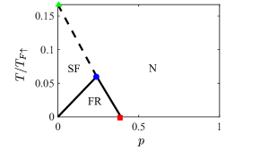
Figure 2: Phase diagram of the two-component Fermi mixture in the unitarity limit, consisting of the superfluid phase (SF), the forbidden region (FR), and the normal phase (N) in the coordinates of $p$ and $T/T_{F\uparrow}$. The dashed line denotes the approximate phase boundary beyond the tricritical temperature $T_{c3}$. Square (red): quantum critical point from Ref. Gubbels and Stoof (2008) at polarization $p_{c0}=0.39$. Circle (blue): the tricritical point from Ref. Gubbels and Stoof (2008), at polarization $p_{c3}=0.24$ and temperature $T_{c3}=0.06T_{F\uparrow}$. Triangle (green): critical temperature $T_{c}=0.167T_{F}$ at zero polarization from Ref. Ku et al. (2012).

II.2 Phenomenological mean-field model

To carry out the calculations, we employ the Blonder-Tinkham-Klapwijk (BTK) framework originally introduced to describe normal-superconductor interfaces Blonder et al. (1982). The BTK framework describes the superconducting state using a mean-field theory, and calculates the transport of quasiparticles across a step function in the superconducting or superfluid gap, with a delta-function potential at the interface. Despite being based on mean-field theory, the BTK framework has been successfully used to model interfaces with high-$T_{c}$ superconductors Tanaka and Kashiwaya (1995); Fischer et al. (2007); Bouscher et al. (2020), and has been extended to spin-imbalanced unitary Fermi gases Van Schaeybroeck and Lazarides (2007, 2009); Parish and Huse (2009). Similar to Refs. Van Schaeybroeck and Lazarides (2007, 2009); Parish and Huse (2009), we employ a phenomenological mean-field model to describe excitations of the strongly interacting fermion system, and obtain transport properties by studying the scattering of quasiparticles by the NS interface. To provide the most accurate predictions possible within a phenomenological model, we choose the model parameters to fit state-of-the-art experimental Shin et al. (2008); Schirotzek et al. (2008); Nascimbène et al. (2010, 2011); Ku et al. (2012); Zürn et al. (2013); Hoinka et al. (2017); Yan et al. (2019) and theoretical Gubbels and Stoof (2008); Combescot and Giraud (2008); Prokof’ev and Svistunov (2008); Mora and Chevy (2010) determinations of thermodynamic and spectroscopic quantities in the unitary Fermi gas. A variety of other approaches have recently been pursued to study non-equilibrium dynamics of strongly interacting fermions, including the time-dependent superfluid local density approximation (SLDA) Bulgac and Forbes (2011); Forbes et al. (2011); Bulgac et al. (2012); Bulgac (2013); Wlazłowski et al. (2018); Magierski et al. (2019); Kopyciński et al. (2021); Hossain et al. (2022), Keldysh Green’s function methods Kawamura et al. (2020); Wang et al. (2014); Liu et al. (2017), time-dependent Ginzburg-Landau theory Scherpelz et al. (2014), and linear response theory Enss and Haussmann (2012); Wlazłowski et al. (2013); Sekino et al. (2020); Frank et al. (2020).

We apply a model Hamiltonian of the form Van Schaeybroeck and Lazarides (2009):

$$H=\sum_{\sigma} \int\mathrm{d}^{3}r\,\hat{\psi}_{\sigma}^{{\dagger}}\,H^{(0)}_{\sigma}\,\hat{\psi}_{\sigma}$$ (2)

$$+ \int\mathrm{d}^{3}r\left[\,\Delta(z)\,\hat{\psi}_{\uparrow}^{{\dagger}}\,\hat{\psi}_{\downarrow}^{{\dagger}}+\Delta^{*}(z)\,\hat{\psi}_{\downarrow}\,\hat{\psi}_{\uparrow}\right]$$

Here $H^{(0)}_{\sigma}$ is the single-particle grand canonical Hamiltonian for spin $\sigma$:

$$H^{(0)}_{\sigma}(z)=-\frac{\hbar^{2}\nabla^{2}}{2m_{\sigma}(z)}-\mu_{\sigma}(z)+U_{\sigma}(z)+\Lambda\delta(z)$$ (3)

The chemical potentials $\mu_{\sigma}$, effective masses $m_{\sigma}$, gap $\Delta$, and Hartree energies $U_{\sigma}$ are modeled as step functions that are discontinuous across the normal-superfluid interface:

$$\mu_{\sigma}(z)=\begin{cases}\mu_{N\sigma},&\text{for }z<0\\ \mu_{S\sigma},&\text{for }z>0\end{cases}$$ (4)

and

$$U_{\sigma}(z)=\begin{cases}U_{N\sigma},&\text{for }z<0\\ U_{S\sigma},&\text{for }z>0\end{cases}$$ (5)

Here $\sigma=\uparrow,\downarrow$ denotes the spin. In a given region (N or S), we also express the chemical potentials of spin up and down in terms of their mean value $\mu$ and deviation $h$ (also called the Zeeman field):

$$\mu_{N}=(\mu_{N\uparrow}+\mu_{N\downarrow})/2 h_{N}=(\mu_{N\uparrow}-\mu_{N\downarrow})/2$$ (6)

$$\mu_{S}=(\mu_{S\uparrow}+\mu_{S\downarrow})/2 h_{S}=(\mu_{S\uparrow}-\mu_{S\downarrow})/2$$ (7)

In the superfluid region, a similar parametrization proves useful for the Hartree energies:

$$U_{S}=(U_{S\uparrow}+U_{S\downarrow})/2 U_{h}=(U_{S\uparrow}-U_{S\downarrow})/2$$ (8)

Theoretical Carlson and Reddy (2005); Magierski et al. (2009); Haussmann et al. (2009) and experimental Schirotzek et al. (2008); Stewart et al. (2008) studies show that the peak of the spectral function in the unitary Fermi gas is well-described by an effective mass, Hartree energy, and gap parameter. We therefore choose the masses, Hartree energies, and gap to reproduce known properties of the unitary Fermi gas. Without loss of generality, we consider the case where the majority is spin up. Minority-spin quasiparticles in the spin-imbalanced normal region acquire an effective mass $m_{\downarrow}(z<0)=m^{*}$, where $m^{*}$ is the polaron mass Combescot and Giraud (2008). We set the effective mass $m_{\uparrow}(z<0)$ of the majority spin equal to the bare mass $m$ in the spin-imbalanced normal region Nascimbène et al. (2010); Mora and Chevy (2010). Likewise, we set the effective masses of both spin states equal to the bare mass in the superfluid phase, in accordance with quantum Monte Carlo calculations at low temperature Magierski et al. (2009). For simplicity, we do not account for the modified effective mass of quasiholes in the superfluid Stewart et al. (2008); Haussmann et al. (2009). While a general mean-field Hamiltonian contains Hartree energy terms de Gennes (1989), the Hartree terms vanish at the mean-field level for the unitary Fermi gas, and generally for contact interactions in the continuum limit Haussmann et al. (2007). In that sense, the Hartree energies in our model Hamiltonian represent effects beyond the mean-field level.

As mentioned above, we treat $\Delta$ and the $U_{\sigma}$ as parameters in the Hamiltonian, and choose their values to match existing experimental data and first-principles calculations, similar to the treatment of the unitary Fermi gas in Refs.  Van Schaeybroeck and Lazarides (2009); Parish and Huse (2009). Our procedure therefore differs from weak-coupling self-consistent mean-field theory, where $\Delta$ and $U_{\sigma}$ would be defined in terms of expectation values of the field operators, and determined using gap and number equations. The gap $\Delta$ in our calculation is therefore the spectral gap parameter rather than the superfluid order parameter Mueller (2017). We let $\Delta=0$ in the spin-imbalanced normal phase Mueller (2011). For the superfluid phase, we set $\Delta/\mu_{S}=1.25$ based on experimentally measured values for the unitary Fermi gas Schirotzek et al. (2008); Ku et al. (2012); Zürn et al. (2013); Hoinka et al. (2017). The latter quantity has an experimental uncertainty on the order of 5-10% due to uncertainty on the gap. For simplicity, we apply the same value in the presence of spin imbalance in the superfluid.

To diagonalize the model Hamiltonian (2), we apply a Bogoliubov transformation to the field operators:

$$\hat{\psi}_{\uparrow}(\mathbf{r})=\sum_{n}u_{n\uparrow}(\mathbf{r})\,\hat{\gamma}_{n\alpha}-v_{n\uparrow}^{*}(\mathbf{r})\,\hat{\gamma}_{n\beta}^{\dagger}$$ (9)

$$\hat{\psi}_{\downarrow}(\mathbf{r})=\sum_{n}u_{n\downarrow}(\mathbf{r})\,\hat{\gamma}_{n\beta}+v_{n\downarrow}^{*}(\mathbf{r})\,\hat{\gamma}_{n\alpha}^{{\dagger}}$$ (10)

The Bogoliubov operators satisfy fermionic anti-commutation relations,

$$\{\hat{\gamma}_{n\sigma},\hat{\gamma}_{n^{\prime}\sigma^{\prime}}^{{\dagger}}\}=\delta_{nn^{\prime}}\delta_{\sigma\sigma^{\prime}}$$ (11)

The Hamiltonian (2) is diagonalized when the Bogoliubov modes satisfy the Bogoliubov-de Gennes (BdG) equations Van Schaeybroeck and Lazarides (2007, 2009):

$$\begin{pmatrix}H^{(0)}_{\uparrow}&\Delta(z)\\ \Delta^{*}(z)&-H^{(0)}_{\downarrow}\end{pmatrix}\,\begin{pmatrix}u_{n\uparrow}\\ v_{n\downarrow}\end{pmatrix}=E_{n\alpha}\begin{pmatrix}u_{n\uparrow}\\ v_{n\downarrow}\end{pmatrix}$$ (12)

$$\begin{pmatrix}H_{\downarrow}^{(0)}&\Delta(z)\\ \Delta^{*}(z)&-H_{\uparrow}^{(0)}\end{pmatrix}\,\begin{pmatrix}u_{n\downarrow}\\ v_{n\uparrow}\end{pmatrix}=E_{n\beta}\begin{pmatrix}u_{n\downarrow}\\ v_{n\uparrow}\end{pmatrix}$$ (13)

In terms of the Bogoliubov operators, the Hamiltonian becomes:

$$H=E_{gs}+\sum_{n}\left(E_{n\alpha}\hat{\gamma}_{n\alpha}^{{\dagger}}\hat{\gamma}_{n\alpha}+E_{n\beta}\hat{\gamma}_{n\beta}^{{\dagger}}\hat{\gamma}_{n\beta}\right)$$ (14)

Here $E_{gs}$ is the ground-state energy and $E_{n\alpha}$ and $E_{n\beta}$ are the single-particle excitation energies

For clarity, and to introduce our notation, below we review the solutions to the BdG equations in the presence of spin imbalance Van Schaeybroeck and Lazarides (2009, 2007). We will refer to the solutions of (12) and (13) as the $\alpha$ and $\beta$ branch, respectively. We denote momentum in the normal-phase by $k$ and in the superfluid by $q$.

In the normal phase ($\Delta=0$), the volume-normalized eigenfunctions on both branches have the form:

$$\begin{pmatrix}u_{\mathbf{k}}(\mathbf{r})\\ v_{\mathbf{k}}(\mathbf{r})\end{pmatrix}=\frac{1}{\sqrt{\Omega}}\begin{pmatrix}1\\ 0\end{pmatrix}\,e^{i\mathbf{k}\cdot\mathbf{r}}\,,\frac{1}{\sqrt{\Omega}}\begin{pmatrix}0\\ 1\end{pmatrix}\,e^{i\mathbf{k}\cdot\mathbf{r}}$$ (15)

where $\Omega$ is the quantization volume. The first solution requires $\hbar^{2}k^{2}/(2m_{\sigma})>\mu_{N\sigma}-U_{N\sigma}$ to give a positive excitation energy, and corresponds to a particle excitation. Likewise, the second solution requires $\hbar^{2}k^{2}/(2m_{\sigma})<\mu_{N\sigma}-U_{N\sigma}$ to give a positive excitation energy, and corresponds to a hole excitation. In the $\alpha$ branch (12), the particle solution excites purely $\psi_{\uparrow}$ (i.e. a spin-up atom in an atomic system), and the hole solution excites $\psi_{\downarrow}$, while the reverse holds in the $\beta$ branch (13).

The BdG equations for a translationally invariant superfluid admit plane wave solutions of the form:

$$\begin{pmatrix}u_{\mathbf{q}}(\mathbf{r})\\ v_{\mathbf{q}}(\mathbf{r})\end{pmatrix}=\frac{1}{\sqrt{\Omega}}\begin{pmatrix}u(\mathbf{q})\\ v(\mathbf{q})\end{pmatrix}\,e^{i\mathbf{q}\cdot\mathbf{r}}$$ (16)

The positive eigenvalues of (12) and (13) give the energies:

$$E_{\alpha}=E_{s}-h_{S}+U_{h}>0$$ (17)

$$E_{\beta}=E_{s}+h_{S}-U_{h}>0$$ (18)

where

$$E_{s}=\sqrt{\xi_{s}^{2}+|\Delta|^{2}}\quad\text{and}\quad\xi_{s}=\left|\frac{\hbar^{2}q^{2}}{2m}-\mu_{S}+U_{S}\right|$$ (19)

At a given energy $E_{\alpha(\beta)}$, equations (17) and (18) admit up to two solutions for the magnitude $q$ of the wavevector. The smaller value $q_{h}$ corresponds to quasihole excitations while the larger value $q_{p}$ corresponds to quasiparticle excitations. We give explicit expressions for the wavevectors as functions of energy in Appendix B. The eigenmodes in both the $\alpha$ and $\beta$ branches can then be written:

$$\begin{pmatrix}u(\mathbf{r})\\ v(\mathbf{r})\end{pmatrix}=\frac{1}{\sqrt{\Omega}}\begin{pmatrix}u_{0}\\ v_{0}\end{pmatrix}\,e^{i\mathbf{q}_{p}\cdot\mathbf{r}},\,\frac{1}{\sqrt{\Omega}}\begin{pmatrix}v_{0}\\ u_{0}\end{pmatrix}\,e^{i\mathbf{q}_{h}\cdot\mathbf{r}}$$ (20)

corresponding to quasiparticles and quasiholes, respectively. Here the quantities $u_{0}$ and $v_{0}$ are:

$$u_{0}=\sqrt{\frac{1}{2}\,\left(1+\frac{\xi_{s}}{E_{s}}\right)}\quad\text{and}\quad v_{0}=\sqrt{\frac{1}{2}\,\left(1-\frac{\xi_{s}}{E_{s}}\right)}$$ (21)

which are functions of energy $E_{\alpha(\beta)}$ on branch $\alpha(\beta)$. Because $u_{0}\geq v_{0}$, particle-like excitations on the $\alpha$ branch involve mostly $\psi_{\uparrow}$ (i.e. spin-up atoms) while hole-like excitations involve mostly $\psi_{\downarrow}$, while the reverse holds on the $\beta$ branch.

To find the Hartree energies $U_{\sigma}$, we equate the expression for the densities $n_{\sigma}=\langle\hat{\psi}^{\dagger}_{\sigma}\hat{\psi}_{\sigma}\rangle$ from our phenomenological mean-field model to the expected densities based on studies of the equation of state of the unitary Fermi gas. In particular, we consider the normal phase Nascimbène et al. (2010); Mora and Chevy (2010), balanced superfluid Ku et al. (2012); Nascimbène et al. (2010) , and critically polarized superfluid Gubbels and Stoof (2008). Details of our procedure for determining the Hartree energies are given in Appendix A.

II.3 Degrees of freedom

At a given temperature $T$, the two-region system in local equilibrium has four degrees of freedom, namely the four chemical potentials: $\mu_{N\uparrow}$, $\mu_{N\downarrow}$, $\mu_{S\uparrow}$, and $\mu_{S\downarrow}$. We non-dimensionalize all energies by dividing by $\mu_{S}$. The three resulting dimensionless parameters are $\mu_{N}/\mu_{S}$, $h_{N}/\mu_{S}$, and $h_{S}/\mu_{S}$. In principle, the instantaneous transport currents can be calculated for arbitrary values of those parameters. We consider a few specific cases.

We consider two cases for $\mu_{N}/\mu_{S}$. In the first case, we consider $\mu_{N}=\mu_{S}$. The pressure in the normal and superfluid regions will be different in this case. Experimentally, the pressure differential can be supported by maintaining a non-zero barrier height between the regions. Therefore, in this case we carry out the calculation in the presence of a non-zero tunneling barrier. Experimentally, arbitrary ratios of $\mu_{N}/\mu_{S}$ can be achieved by tuning the densities in the two regions, for example by moving one of the outer walls of the trap.

In the second case, we choose $\mu_{N}/\mu_{S}$ for a given $T/\mu_{S}$ to achieve mechanical equilibrium. Experimentally, this would describe a situation where the barrier between the regions has been removed and the system has had sufficient time to reach mechanical equilibrium, while still being out of chemical equilibrium Sommer et al. (2011a).

After fixing $\mu_{N}/\mu_{S}$, we choose the two remaining degrees of freedom, $h_{N}/\mu_{S}$ and $h_{S}/\mu_{S}$. We consider two specific cases for $h_{S}/\mu_{S}$: a spin-balanced superfluid ($h_{S}=0$) or a critically polarized superfluid ($h_{s}=h_{c}$). In each case, we consider the full range of $h_{N}$, and calculate the transport currents as functions of $h_{N}$.

Chemical potential differences drive particle transport. We therefore define $\delta\mu_{\sigma}$ as the chemical potential differences across the interface:

$$\delta\mu_{\uparrow}=\mu_{N\uparrow}-\mu_{S\uparrow}\quad\text{and}\quad\delta\mu_{\downarrow}=\mu_{S\downarrow}-\mu_{N\downarrow}$$ (22)

The choice of signs in (22) ensures that $\delta\mu_{\sigma}\geq 0$. In the special case of $\mu_{N}=\mu_{S}$, we have $\delta\mu_{\uparrow}=\delta\mu_{\downarrow}$. The relation between the $\delta\mu_{\sigma}$ and $h_{N}$ and $h_{S}$ depends on the equation of state and is plotted for our model in Appendix F. Experimentally, one typically measures density rather than chemical potential, so we also plot the polarization $p_{N}$ of the normal region versus $h_{N}$ in Appendix F.

III Scattering formulation and Current densities

III.1 Scattering states and coefficients

Transport across the normal-superfluid interface can be described in terms of quasiparticle reflection and transmission coefficients Blonder et al. (1982). Scattering of quasiparticles at the normal-superfluid interface of a spin-imbalanced Fermi gas has been discussed previously in Refs. Van Schaeybroeck and Lazarides (2007, 2009); Parish and Huse (2009). We extend previous results by including the Hartree energies and polaron effective mass in the scattering problem, and by using the resulting scattering coefficients to calculate the currents of spin up and spin down fermions across the interface.

To describe scattering at the normal-superfluid interface, we employ energy normalization with respect to the $z$-component of the momentum, rather than the volume normalization of Section II.2. Energy normalization is helpful when dealing with multiple scattering channels having potentially different group velocities. Moving from the single-region solutions of Section II.2 to an interface problem also changes the Bogoliubov modes into scattering solutions that obey boundary conditions at the interface. We parameterize the scattering states in terms of their total energy and transverse momentum, which are both conserved, as well as the incident (in) channel of the scattering process. The $\alpha$ and $\beta$ branches each have four channels, corresponding to a particle or hole incident on the interface from the left or right. Note that the $\alpha$ and $\beta$ branches have no cross-coupling due to conservation of spin de Jong and Beenakker (1995).

We express the total current densities of spin up and spin down in terms of the contributions of each Bogoliubov mode:

$$J_{\sigma}= \frac{1}{A}\sum_{n,\,\mathbf{k}_{\perp}}\int\mathrm{d}E\,\left(j_{\sigma n\alpha}+j_{\sigma n\beta}\right)$$ (23)

Here $n\in\{Lp,Lh,Rp,Rh\}$ runs over the four scattering channels (particle incident from the left, hole incident from the left, particle incident from the right, and hole incident from the right, respectively), $\mathbf{k}_{\perp}$ is the transverse momentum, and $E$ is the energy. The cross-sectional area $A$ cancels upon converting the sum on $\mathbf{k}_{\perp}$ to an integral. In terms of the energy-normalized mode functions, the spin-up current per unit energy from each mode is given by:

$$j_{\uparrow n\alpha}= \frac{\hbar}{2im}\left(\frac{\partial u_{n\uparrow}}{\partial z}u_{n\uparrow}^{*}-\frac{\partial u_{n\uparrow}^{*}}{\partial z}u_{n\uparrow}\right)\,f_{n\alpha}$$ (24)

$$j_{\uparrow n\beta}= -\frac{\hbar}{2im}\left(\frac{\partial v_{n\uparrow}}{\partial z}v_{n\uparrow}^{*}-\frac{\partial v_{n\uparrow}^{*}}{\partial z}v_{n\uparrow}\right)\,(1-f_{n\beta})$$ (25)

Similarly, the contributions to the spin-down current are:

$$j_{\downarrow n\beta}= \frac{\hbar}{2im^{*}}\left(\frac{\partial u_{n\downarrow}}{\partial z}u_{n\downarrow}^{*}-\frac{\partial u_{n\downarrow}^{*}}{\partial z}u_{n\downarrow}\right)\,f_{n\beta}$$ (26)

$$j_{\downarrow n\alpha}= -\frac{\hbar}{2im^{*}}\left(\frac{\partial v_{n\downarrow}}{\partial z}v_{n\downarrow}^{*}-\frac{\partial v_{n\downarrow}^{*}}{\partial z}v_{n\downarrow}\right)\,(1-f_{n\alpha})$$ (27)

Here $f_{n\alpha}$ and $f_{n\beta}$ are the occupation probabilities of the Bogoliubov modes in the $\alpha$ and $\beta$ branches, respectively. Note that the occupation probabilities depend on $E$, and the mode functions depend on $E$ and $\mathbf{k}_{\perp}$.

Under non-equilibrium conditions, the left and right regions will have different chemical potentials for a given spin. When solving the scattering problem, we employ the technique introduced in Ref. Blonder et al. (1982) of referencing all energies to the superfluid-side chemical potentials, and accounting for the non-equilibrium conditions through the quasiparticle distribution functions $f_{n}$. We give explicit expressions for the distribution functions in Appendix C.

We now express the Bogoliubov modes in terms of reflection and transmission coefficients. We write the mode functions for the $\alpha$ and $\beta$ branches as

$$\psi_{n\alpha}=\begin{pmatrix}u_{n\uparrow}\\ v_{n\downarrow}\end{pmatrix}\quad\text{and}\quad\psi_{n\beta}=\begin{pmatrix}u_{n\downarrow}\\ v_{n\uparrow}\end{pmatrix}$$ (28)

for the four channels $n\in\{Lp,Lh,Rp,Rh\}$. For each branch, we construct scattering states in terms of in and out states, which we formally assemble into vectors (dropping the $\alpha$ and $\beta$ subscripts):

$$\bm{\psi}^{in(out)}=\begin{pmatrix}\psi_{Lp}\\ \psi_{Lh}\\ \psi_{Rp}\\ \psi_{Rh}\end{pmatrix}^{in(out)}$$ (29)

The scattering states in each of the four channels are expressed in terms of the in and out states and the $S$ matrix:

$$\psi_{n}=\bm{\psi}^{in}\cdot\bm{e}_{n}+\bm{\psi}^{out}\cdot S\bm{e}_{n}$$ (30)

where $n$ is the channel index, $\bm{e}_{n}$ is the $n$-th unit vector in $\mathbb{R}^{4}$, and the $S$ matrix for either branch consists of 16 scattering coefficients:

$$S=\begin{pmatrix}r_{pp}^{A}&r_{ph}^{B}&t_{pp}^{C}&t_{ph}^{D}\\ r_{hp}^{A}&r_{hh}^{B}&t_{hp}^{C}&t_{hh}^{D}\\ t_{pp}^{A}&t_{ph}^{B}&r_{pp}^{C}&r_{ph}^{D}\\ t_{hp}^{A}&t_{hh}^{B}&r_{hp}^{C}&r_{hh}^{D}\end{pmatrix}$$ (31)

The labels $A$, $B$, $C$, and $D$ refer to the four incident scattering channels $Lp$, $Lh$, $Rp$, and $Rh$, respectively.

For the $\alpha$ branch, the in and out states of a particle in the left (normal) region are:

$$\psi_{Lp\alpha}^{in(out)}=\sqrt{\frac{m}{2\pi\hbar^{2}k_{p\uparrow}}}\begin{pmatrix}1\\ 0\end{pmatrix}e^{\pm ik_{p\uparrow}z}e^{i\mathbf{k_{\perp}}\cdot\mathbf{r}}\theta(-z)$$ (32)

For a hole in the left region, they are:

$$\psi_{Lh\alpha}^{in(out)}=\sqrt{\frac{m^{*}}{2\pi\hbar^{2}k_{h\downarrow}}}\begin{pmatrix}0\\ 1\end{pmatrix}e^{\mp ik_{h\downarrow}z}e^{i\mathbf{k_{\perp}}\cdot\mathbf{r}}\theta(-z)$$ (33)

And for the right region:

$$\psi_{Rp\alpha}^{in(out)}=\sqrt{\frac{m\,E_{s}/\xi_{s}}{2\pi\hbar^{2}q_{p\alpha}}}\begin{pmatrix}u_{0}\\ v_{0}\end{pmatrix}e^{\mp iq_{p\alpha}z}e^{i\mathbf{k_{\perp}}\cdot\mathbf{r}}\theta(z)$$ (34)

$$\psi_{Rh\alpha}^{in(out)}=\sqrt{\frac{m\,E_{s}/\xi_{s}}{2\pi\hbar^{2}q_{h\alpha}}}\begin{pmatrix}v_{0}\\ u_{0}\end{pmatrix}e^{\pm iq_{h\alpha}z}e^{i\mathbf{k_{\perp}}\cdot\mathbf{r}}\theta(z)$$ (35)

Here the upper and lower signs in the exponentials correspond to the in and out states, respectively, and $\theta(z)$ is the Heaviside step function. The wavevectors $k_{p\uparrow}$, $k_{h\downarrow}$, $q_{p\alpha}$, and $q_{h\alpha}$ are the magnitudes of the $z$ components of the wavevectors of particle and hole excitations on the $\alpha$ branch in the normal and superfluid phases; their dependence on the energy and transverse momentum is given in Appendix B. Expressions for the $\beta$ branch in and out states can be obtained by replacing $\alpha\rightarrow\beta$, $\uparrow\leftrightarrow\downarrow$ in (32)-(35) and $m\leftrightarrow m^{*}$ in (32) and (33).

The scattering coefficients are obtained by imposing boundary conditions on the scattering states (30) at the interface. The mode functions must be continuous across the interface: $\psi_{n}(z\rightarrow 0^{-})=\psi_{n}(z\rightarrow 0^{+})$. For the $\alpha$ branch, the derivatives satisfy:

$$\left.\frac{\partial\psi_{n\alpha}}{\partial z}\right|_{z\rightarrow 0^{+}}-\left.\begin{pmatrix}1&0\\ 0&m/m^{*}\end{pmatrix}\frac{\partial\psi_{n\alpha}}{\partial z}\right|_{z\rightarrow 0^{-}}=k_{\Lambda}\psi_{n\alpha}(0)$$ (36)

where $k_{\Lambda}$ is defined in Eqn (1). For the $\beta$ branch, the derivatives satisfy:

$$\left.\frac{\partial\psi_{n\beta}}{\partial z}\right|_{z\rightarrow 0^{+}}-\left.\begin{pmatrix}m/m^{*}&0\\ 0&1\end{pmatrix}\frac{\partial\psi_{n\beta}}{\partial z}\right|_{z\rightarrow 0^{-}}=k_{\Lambda}\psi_{n\beta}(0)$$ (37)

Note that we obtain the boundary conditions (36) and (37) using the Hermitian kinetic energy operator ordering $\frac{1}{2}\hat{p}\,m_{\sigma}^{-1}(z)\hat{p}$ from effective mass theory BenDaniel and Duke (1966); Einevoll (1990); Cavalcante et al. (1997).

Full expressions for the resulting scattering coefficients are given in Appendix E. We find that the $S$ matrix is unitary, $S^{\dagger}S=1$, as required by conservation of probability. We also find that the transpose satisfies $S(\Delta)^{T}=S(\Delta^{*})$, as required by time-reversal symmetry. As $S$ has the property $S(\Delta)^{*}=S(\Delta^{*})$, it follows that $S$ is Hermitian: $S^{\dagger}=S$. The unitarity and Hermiticity of $S$ will assist in simplifying the expressions for the currents. In particular, the coefficients for channels $C$ and $D$ (excitation incident from the right) can be written in terms of the coefficients for channels $A$ and $B$ (excitation incident from the left), allowing us to express the currents in terms of the coefficients for channels $A$ and $B$.

The coefficient $r^{A}_{hp}$ for the $\alpha$ branch (which we will denote as $r^{A}_{hp_{\alpha}}$) represents an Andreev reflection process, where a spin-up particle from the normal region is reflected as a spin-down hole. Likewise, $r^{B}_{ph_{\alpha}}$ describes the reversed process, or reverse Andreev reflection, where a spin-down hole is reflected as a spin-up particle. Meanwhile, the coefficients $r^{C}_{hp}$ and $r^{D}_{ph}$ describe Andreev-type reflection of excitations incident from the superfluid region. Physically, a Cooper pair is created or annihilated in the superfluid during Andreev reflection to conserve particle number. Andreev reflections therefore transport mass across the interface. In the forward Andreev reflection $r^{A}_{hp}$, a spin-up particle and a spin-down particle leave the normal region and a Cooper pair appears in the superfluid. In reverse Andreev reflection $r^{B}_{ph}$, a Cooper pair disappears and the normal region gains a spin up and a spin down particle. Andreev reflection does not transport spin, however, as the total spin in each region remains unchanged. Moreover, unlike a quasiparticle transmission process, Andreev reflection does not create or annihilate a single-particle excitation in the superfluid, and therefore can occur at energies within the superfluid excitation gap.

III.2 Current densities

Employing the scattering states in the expressions for the current contributions (24)-(27) gives general expressions for the currents in terms of the $S$ matrix elements. In particular, we are interested in the net (mass) current and the spin current:

$$J^{\text{net}}=J_{\uparrow}+J_{\downarrow}\quad\text{and}\quad J^{\text{spin}}=J_{\uparrow}-J_{\downarrow}$$ (38)

Depending on the values of $E$ and $k_{\perp}$, some scattering channels can become closed, leading to different scattering regimes as described in Refs. Van Schaeybroeck and Lazarides (2007, 2009). Within intervals of $E$ and $k_{\perp}$ where all the channels are open (denoted Regime I in Appendix D), the contributions to the net and spin currents from the $\alpha$ branch are given by:

$$j_{\alpha}^{\text{net}}=\frac{1}{h}\left\{(1-|r_{pp_{\alpha}}^{A}|^{2}+|r_{hp_{\alpha}}^{A}|^{2})[f(E_{\alpha}-\delta\mu_{\uparrow})-f(E_{\alpha})]-(1-|r_{hh_{\alpha}}^{B}|^{2}+|r_{ph_{\alpha}}^{B}|^{2})[f(E_{\alpha}-\delta\mu_{\downarrow})-f(E_{\alpha})]\right\}$$ (39)

$$j_{\alpha}^{\text{spin}}=\frac{1}{h}\left\{(1-|r_{pp_{\alpha}}^{A}|^{2}-|r_{hp_{\alpha}}^{A}|^{2})[f(E_{\alpha}-\delta\mu_{\uparrow})-f(E_{\alpha})]+(1-|r_{hh_{\alpha}}^{B}|^{2}-|r_{ph_{\alpha}}^{B}|^{2})[f(E_{\alpha}-\delta\mu_{\downarrow})-f(E_{\alpha})]\right\}$$ (40)

The $\beta$ branch contributions are:

$$j_{\beta}^{\text{net}}=\frac{1}{h}\left\{(1-|r_{pp_{\beta}}^{A}|^{2}+|r_{hp_{\beta}}^{A}|^{2})[f(E_{\beta}+\delta\mu_{\downarrow})-f(E_{\beta})]-(1-|r_{hh_{\beta}}^{B}|^{2}+|r_{ph_{\beta}}^{B}|^{2})[f(E_{\beta}+\delta\mu_{\uparrow})-f(E_{\beta})]\right\}$$ (41)

$$j_{\beta}^{\text{spin}}=\frac{1}{h}\left\{(1-|r_{pp_{\beta}}^{A}|^{2}-|r_{hp_{\beta}}^{A}|^{2})[f(E_{\beta})-f(E_{\beta}+\delta\mu_{\downarrow})]-(1-|r_{hh_{\beta}}^{B}|^{2}-|r_{ph_{\beta}}^{B}|^{2})[f(E_{\beta}+\delta\mu_{\uparrow})-f(E_{\beta})]\right\}$$ (42)

In regimes where a scattering channel is closed, the corresponding scattering coefficients drop out of the expressions for the currents. Appendix D describes the regimes in more detail.

The current density integrands (39)-(42) show that the contributions from the $\beta$ branch are small compared to the $\alpha$ branch. Since $E_{\alpha}$, $E_{\beta}$, $\delta\mu_{\uparrow}$ and $\delta\mu_{\downarrow}$ are positive, all the Fermi functions in the $\beta$ currents have positive arguments, while some in the $\alpha$ currents can have negative arguments. With positive arguments, the Fermi function quickly drops to zero, leading to vanishing results for the $\beta$ currents. The $\beta$ branch was also found to have a small contribution to heat current at the interface in Ref. Van Schaeybroeck and Lazarides (2007, 2009)

The dominance of the $\alpha$ branch results from the polarization of the normal phase. Creating a large normal (non-Andreev) current of spin $\sigma$ in the $\alpha$ branch requires $\delta\mu_{\sigma}\geq E_{\alpha\mathrm{min}}$, where $E_{\alpha\mathrm{min}}$ is the minimum of $E_{\alpha}$. As discussed in the next section, this can be achieved sufficiently far from equilibrium. On the other hand, because the $\beta$ branch consists of spin up holes and spin down particles, a large normal current in the $\beta$ branch requires $\delta\mu_{\sigma}\leq-E_{\alpha\mathrm{min}}$, which is impossible since $\delta\mu_{\sigma}\geq 0$. In addition, as mentioned earlier, we apply the superfluid chemical potentials $\mu_{S\sigma}$ to the normal side when solving the scattering problem, and implement non-equilibrium through the quasiparticle distribution functions. Consequently, on the normal side, the density of spin-up particles formally exceeds the density of spin-up holes, and vice versa for spin down, so that the $\alpha$ branch accounts for the majority of excitations on the normal side. In our final calculations, we confirm that for temperatures below $0.3\mu_{S}$, the $\alpha$ branch accounts for at least 99% of the current.

IV Results and Discussion

IV.1 Interface away from mechanical equilibrium

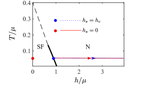
Figure 3: Thermodynamic states considered, for the case $\mu_{N}=\mu_{S}$. For the sub-case $h_{s}=0$ (unpolarized superfluid), the red dot indicates the state of the superfluid region while the red line indicates the allowed states of the normal region, given the temperature $T=0.05\mu_{S}$ and the condition $\mu_{N}=\mu_{S}$. For the other sub-case, $h_{s}=h_{c}$ (critically polarized superfluid), the blue dot indicates the state of the superfluid region while the blue dashed line indicates the allowed states of the normal region. The solid black and black dashed curves show the normal-superfluid phase boundary above and below the tricritical point, respectively. The maximum value of $h_{N}/\mu_{N}$ on the red solid and blue dotted lines correspond to $p_{N}=0.99$, while the minimum $h_{N}/\mu_{N}$ corresponds to the critical polarization in the normal phase of $p_{Nc}=0.34$ at $T/\mu_{N}=T/\mu_{s}=0.05$.

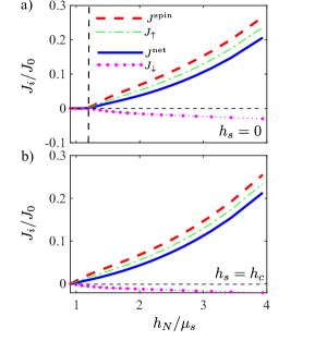
Figure 4: Net, spin, spin-up and spin-down current densities for the case $\mu_{N}=\mu_{S}$ as functions of $h_{N}/\mu_{S}$, under the conditions: (a) $h_{S}=0$, and (b) $h_{S}=h_{c}$. For both plots, the temperature is $T=0.05\mu_{S}$. The vertical dashed line in (a) denotes the $h_{N}$ value at which $\delta\mu_{\uparrow}=\delta\mu_{\downarrow}=E_{min}$, corresponding to normal-region polarization $p_{N}=0.44$. The horizontal dashed line in both plots is the $J_{i}=0$ line. The horizontal axes start at $h_{N}=h_{c}(T=0.05\mu_{S})=0.91\mu_{s}$.

In this section, we consider the case where the system is out of mechanical equilibrium and a Dirac delta potential barrier is applied. We analyze the particular case of $\mu_{N}=\mu_{S}$, and barrier strength $k_{\Lambda}=20k_{s}$, where $k_{s}=2m\mu_{S}/\hbar^{2}$. We consider two different conditions for the superfluid, (1) $h_{S}=0$ for a spin-balanced superfluid, and (2) $h_{S}=h_{c}$ for a maximally polarized superfluid. In both cases, we consider a normal region with chemical potential imbalance $h_{N}$ (equivalently, polarization $p_{N}$) greater than the equilibrium value, so that the system is out of global equilibrium. Figure 3 plots the thermodynamic states under consideration on the phase diagram in terms of $T/\mu$ and $h/\mu$. In both cases, $h_{s}$ is held at a fixed value, while $h_{N}$ is varied from the critical value up to a large value corresponding to a normal-region polarization of $p_{N}=0.99$.

In Fig. 4, we show the instantaneous net and spin currents versus $h_{N}$. The currents are normalized by a factor $J_{0}$, given by:

$$J_{0}=\frac{m\,\mu_{S}^{2}}{4\pi^{2}\,\hbar^{3}}$$ (43)

The currents for the unpolarized superfluid exhibit a threshold at a critical value of $h_{N}$, as shown in Fig. 4(a). To interpret the threshold, we first note that, in the present case where $\mu_{N}=\mu_{S}$, the chemical potential differences (22) satisfy $\delta\mu_{\uparrow}=\delta\mu_{\downarrow}$, as illustrated in Fig. 5. The threshold occurs at the value of $h_{N}$ where $\delta\mu_{\uparrow}$ and $\delta\mu_{\downarrow}$ equal the superfluid minimum excitation energy $E_{min}$. With $E_{min}=\Delta_{0}-h_{S}+U_{h}$, we have $E_{min}(h_{S}=0)=\Delta_{0}=1.25\mu_{s}$ for the unpolarized superfluid, while $E_{min}(h_{S}=h_{c})=0.02\mu_{S}$ for the critically polarized superfluid. Accordingly, the threshold in the critically polarized superfluid, Fig. 4(b), is too small to easily discern. The presence of a threshold implies that the system is metastable when $h_{s}=0$: the system is out of equilibrium, but mass and spin transport are strongly suppressed. Figure 5 shows an example of a situation where the threshold is exceeded, allowing currents to flow.

As mentioned earlier, the spin current results entirely from normal (non-Andreev) transmission processes. Normal current involves the creation or annihilation of an excitation in the superfluid. Efficient creation of excitations in the superfluid at low temperatures requires $\delta\mu_{\uparrow}>E_{\mathrm{min}}$ for spin up excitations, and $\delta\mu_{\downarrow}>E_{\mathrm{min}}$ for spin down (holes). The energy required to excite the superfluid therefore explains the observed threshold in the spin current.

The net current consists, in general, of both normal and Andreev processes. Andreev reflection does not excite the superfluid, and therefore should exhibit no threshold effects. The presence of a threshold in the net current in Fig. 4(a) suggests that the net Andreev current vanishes in this case. To confirm that the Andreev current vanishes, we separate the net current into Andreev and normal components. We identify the Andreev current in the $\alpha$ branch as the sum of the terms in Eq. (39) that are proportional to the Andreev reflection coefficients:

$$j^{\text{Andreev}}_{\alpha}=\frac{2}{h}|r_{hp_{\alpha}}^{A}|^{2}\left[f(E_{\alpha}-\delta\mu_{\uparrow})-f(E_{\alpha}-\delta\mu_{\downarrow})\right]$$ (44)

We have used $|r^{B}_{ph_{\alpha}}|^{2}=|r^{A}_{hp_{\alpha}}|^{2}$ from the hermiticity of the $S$-matrix to simplify the expression. We verify Eq. (44) by considering the net current in the scattering regime where normal transmission is energetically forbidden, denoted Regime II in Appendix D. We find that the net $\alpha$ branch current is given by (44) in Regime II, confirming that it captures the current due to Andreev reflection. In the present case of $\mu_{N}=\mu_{S}$, where $\delta\mu_{\uparrow}=\delta\mu_{\downarrow}$, Eqn. (44) shows that the Andreev contribution to the net current is indeed zero, explaining the sharp threshold observed in the net current.

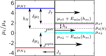
Figure 5: Chemical potentials and current densities across the interface, away from mechanical equilibrium, for parameters $p_{N}=99\%$, and $h_{S}=h_{c}$, $\mu_{N}=\mu_{S}$, $T=0.05\mu_{S}$. The left (right) side of the figure corresponds to the normal (superfluid) region. The horizontal axis is qualitative, showing the directions and relative magnitudes of the currents. The vertical axis shows the chemical potentials quantitatively.

We now discuss a final point of interest regarding the results in Fig. 4. Although $\delta\mu_{\uparrow}=\delta\mu_{\downarrow}$ for $\mu_{N}=\mu_{S}$, the spin-up current in Fig. 4 is much larger than the spin-down current. We attribute this asymmetry to the asymmetry in the dispersion relations between particle-like and hole-like excitations, in both the normal and superfluid phases. While the energy of a particle-like excitation is unbounded, the energy of a hole-like excitation is bounded from above. As a result, when integrating over the total energy $E_{\alpha}$ and transverse kinetic energy $\xi_{\perp}$ to obtain the currents, there are regimes in which hole-like excitations are forbidden in the normal and/or superfluid phase (Appendix D). As a result, the current of hole-like excitations is smaller than the current of particle-like excitations. On the $\alpha$ branch, particle-like excitations result predominantly from excitations of $\psi_{\uparrow}$ (i.e. spin-up atoms), while hole-like excitations result predominantly from $\psi_{\downarrow}$. Consequently, the spin-up current is larger than the spin-down current in this case, despite the equality of the driving chemical potential differences.

IV.2 Interface at mechanical equilibrium

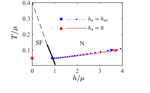
Figure 6: Thermodynamic states considered, for the case of mechanical equilibrium at temperature $T=0.05\mu_{S}$. The maximum value of $h_{N}/\mu_{N}$ on the red solid (blue dotted) line corresponds to $p_{N}=0.96$.

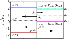
Figure 7: Chemical potentials and schematic current densities across the interface, at mechanical equilibrium, with $p_{N}=0.96$, and $h_{S}=h_{c}$, $T=0.05\mu_{S}$.

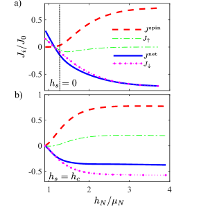
Figure 8: Net, spin, spin-up and spin-down current densities as functions of $h_{N}$, under the conditions: (a) $h_{S}=0$, and (b) $h_{S}=h_{c}$. For both plots, temperature is $T=0.05\mu_{S}$. The dashed vertical line denotes the $h_{N}$ value at which $\delta\mu_{\downarrow}=E_{min}$.

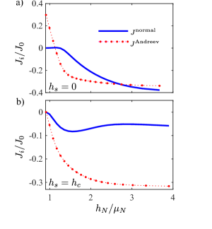
Figure 9: The normal and Andreev contributions to the net current as functions of $h_{N}$, under the conditions: (a) $h_{S}=0$, and (b) $h_{S}=h_{c}$. For both plots, temperature is $T=0.05\mu_{S}$.

In this section, we apply our model to the case where the interface is at mechanical equilibrium and no potential barriers are applied. We consider two conditions for the superfluid region, as in the previous section, (1) $h_{S}=0$ for a spin-balanced superfluid, and (2) $h_{S}=h_{c}$ for a maximally polarized superfluid. We calculate the instantaneous currents as a function of normal-region chemical potential imbalance $h_{N}$ and point out interesting features of the results.

Figure 6 shows the thermodynamic states considered for the normal and superfluid regions on the phase diagram in the case of mechanical equilibrium at temperature $T=0.05\mu_{S}$. The condition of mechanical equilibrium causes $\mu_{N}/\mu_{S}$ to depend on $h_{N}/\mu_{S}$, unlike in the previous section where $\mu_{N}/\mu_{S}$ had a fixed value. As a result, the dimensionless temperature coordinate $T/\mu_{N}$ of the normal region varies with $h_{N}/\mu_{S}$. The values of $T/\mu_{N}$ in Fig. 6 for an unpolarized superfluid ($h_{S}=0$; solid red curve) differ slightly from the case of a critically polarized superfluid ($h_{S}=h_{c}$; dotted blue curve), due to the dependence of the superfluid pressure on polarization.

Figure 7 shows an example of the chemical potentials and current densities at large normal-region polarization, where $\mu_{S}>\mu_{N}$.

In Fig. 8, we show the instantaneous spin and net currents versus $h_{N}$ at $T=0.05\mu_{S}$. As in the previous section, we observe a threshold behavior in the spin current for the unpolarized superfluid ($h_{S}=0$) and no significant threshold for the critically polarized superfluid ($h_{S}=h_{c}$). As before, the threshold occurs when the chemical potential difference for one of the spin states exceeds the minimum excitation energy in the superfluid, which is nearly zero for the critically polarized superfluid. The vertical line in Fig. 8(a) shows the threshold for the spin current in the case of an unpolarized superfluid. The threshold is given by the point at which $\delta\mu_{\downarrow}=E_{min}$, which occurs at a lower polarization than $\delta\mu_{\uparrow}=E_{min}$.

Unlike in Fig. 4, where we considered $\mu_{N}=\mu_{S}$, here the net current does not exhibit a threshold. The absence of a threshold results from a non-zero Andreev current when $\mu_{N}\neq\mu_{S}$. Interestingly, for $h_{s}=0$, the sign of $\mu_{N}-\mu_{S}$ changes as $h_{N}$ is increased, crossing zero before the threshold, where the sign of the net current also changes.

In Fig. 8, the spin-up current is small compared to spin-down current at large normal-region polarization, contrary to what we found in the $\mu_{S}=\mu_{N}$ case. This is because, at large $h_{N}$, where $\mu_{S}>\mu_{N}$, the Andreev current flows from the superfluid into the normal region through reverse Andreev reflection. On the other hand, the normal component of the spin-up current flows in the opposite direction, because $\mu_{N\uparrow}>\mu_{S\uparrow}$. As a result, the normal and Andreev components of the spin-up current nearly cancel. Meanwhile, the normal spin-down current flows in the same direction as the Andreev current, resulting in a larger spin-down current.

To confirm the interpretations described above we decompose the net current into Andreev and normal components. Figure 9 shows that the normal component exhibits a threshold in the $h_{S}=0$ case, while the Andreev component does not. The net current in Fig. 8(a), which is the sum of the normal and Andreev currents in Fig. 9(a), therefore does not have a threshold effect. We further decompose the $\alpha$-branch normal current into spin-up and spin-down components in Fig. 10. The total contributions to these currents entering Eqns. (24) and (27) can be expressed as:

$$j^{\text{normal}}_{\uparrow\alpha}=\frac{1}{h}(|t_{pp_{\alpha}}^{A}|^{2}+|t_{hp_{\alpha}}^{A}|^{2})[f(E_{\alpha}-\delta\mu_{\uparrow})-f(E_{\alpha})]$$ (45)

$$j^{\text{normal}}_{\downarrow\alpha}=-\frac{1}{h}(|t_{hh_{\alpha}}^{B}|^{2}+|t_{ph_{\alpha}}^{B}|^{2})[f(E_{\alpha}-\delta\mu_{\downarrow})-f(E_{\alpha})]$$ (46)

Figure 10 and equations (45) and (46) confirm that the normal spin-up current is positive while the normal spin-down current is negative, as mentioned in the discussion of the relative sizes of the total spin-up and spin-down currents above. Figure 10 also shows that the normal spin-up and spin-down currents each exhibit a threshold in the $h_{S}=0$ case.

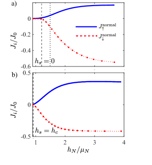
Figure 10: Normal (non-Andreev) contributions to the spin up and spin down currents on the $\alpha$ branch versus $h_{N}$. (a) $h_{S}=0$ (b) $h_{S}=h_{c}$. For both plots, temperature is $T=0.05\mu_{S}$. The dashed vertical line denotes the $h_{N}$ value at which $\delta\mu_{\downarrow}=E_{min}$, while the dotted vertical line indicates $\delta\mu_{\uparrow}=E_{min}$.

Interestingly, the normal spin-up current in Fig. 10 exhibits a threshold at a lower value of $h_{N}$ than expected based on the condition $\delta\mu_{\uparrow}=E_{min}$. This behavior reveals the temperature dependence of the threshold. At finite temperature, the normal current for spin $\sigma$ should become significant when $\delta\mu_{\sigma}\gtrsim E_{min}-k_{B}T$. The threshold will therefore shift to lower polarization. The size of the shift in $h_{N}$ depends on the sensitivity of $\delta\mu_{\sigma}$ to $h_{N}$. As shown in Fig. 14 (Appendix F), $\delta\mu_{\uparrow}$ has a much weaker dependence on $h_{N}$ than does $\delta\mu_{\downarrow}$. Therefore, the threshold value of $h_{N}$ changes by a larger amount for spin up than for spin down. At low temperatures, a first-order Taylor expansion gives the shift of the threshold for spin $\sigma$ as $\Delta h_{N}^{\sigma}\approx-k_{B}T/(d\delta\mu_{\sigma}/dh_{N})$. Using this formula, we confirm that the shift in the spin-up threshold should be significantly larger than the shift in the spin-down threshold. The estimated shift in the spin-down threshold ($\approx-0.06\mu_{N}$) is too small to observe on the scale of Fig. 10. The shift in the spin-up threshold ($\approx-0.3\mu_{N}$) coincidentally brings the spin-up threshold to about the same $h_{N}$ value as the spin-down threshold, in agreement with the observed behavior of the normal currents in Fig. 10(a).

Finally, we note that in both Fig. 4(b) and Fig. 8(b), the spin current is positive when $h_{S}=h_{c}$, and, therefore, increases the polarization in the already maximally polarized superfluid region. The $z>0$ region would have to accommodate the influx of spin through phase separation, implying that the NS interface should advance to $z>0$ and the volume of the critically polarized superfluid should shrink as a function of time.

V Conclusions

In conclusion, we investigated the transport of spin and mass across non-equilibrium normal-superfluid interfaces in the unitary Fermi gas. We found that, when the superfluid region is unpolarized, the spin current is strongly suppressed below a threshold value of the normal-region polarization. The threshold nearly vanishes in the limit of a critically polarized superfluid. Based on these results, we expect that, for intermediate superfluid polarization, the threshold should vary smoothly between the two limiting cases, following the variation of the minimum excitation energy of the partially polarized superfluid. Our results imply that non-equilibrium NS interfaces below threshold can exhibit suppressed spin transport, contributing to the metastability observed experimentally Liao et al. (2011). However, we find that Andreev reflection should allow mass current to flow even below the threshold for spin transport, except when the average chemical potentials of the normal and superfluid regions are equal. Meanwhile, the quantitative values of the transport currents calculated here provide guidance to future experiments on NS interfaces by indicating the magnitudes of the expected currents.

An interesting question for future work will be the long-time evolution of the NS interface. In particular, dissipation will heat the system, and finite spin conductivity will limit the rate of global equilibration. An interesting direction for future work would be to include these effects to predict the finite-time evolution of the non-equilibrium normal-superfluid mixture. Another important challenge for future work will be to incorporate additional beyond-mean-field effects in the transport dynamics. In particular, finite quasiparticle lifetime may soften the threshold for spin transport Srikanth and Raychaudhuri (1992); Fischer et al. (2007), potentially weakening the metastability of the non-equilibrium system. Experimentally, future work can utilize non-equilibrium NS interfaces as a source of current to study bulk spin transport more precisely, and to explore the properties of Fermi gases under non-equilibrium conditions.

Appendix A Hartree energies from thermodynamics

A.1 Polarized normal phase equation of state

We solve for the Hartree energies in the normal phase by equating the atomic densities in the phenomenological mean-field model to the densities given by the known equation of state at the same temperature and chemical potentials. The equation of state for the polarized normal phase is well-described by the following expression for the pressure Nascimbène et al. (2010); Mora and Chevy (2010):

$$P_{N}=P_{0}(\mu_{N\uparrow})+\left(\frac{m^{*}}{m}\right)^{3/2}P_{0}\left(\mu_{N\downarrow}-A\mu_{N\uparrow}\right)$$ (47)

Here $P_{0}\,(\mu)=k_{B}T\lambda_{th}^{-3}F_{3/2}\left(\beta\mu\right)$ is the pressure in an ideal Fermi gas at chemical potential $\mu$, with $\lambda_{th}=\sqrt{2\pi\hbar^{2}/(mk_{B}T)}$, $F_{3/2}(x)$ the complete Fermi-Dirac integral, and $\beta=1/(k_{B}T)$. While we use $k_{B}=1$ for most of the paper, we include $k_{B}$ here for clarity. The polaron parameters are $A=-0.615$ and $m{{}^{*}}/m=1.20$ Nascimbène et al. (2010); Schirotzek et al. (2009); Pilati and Giorgini (2008); Combescot and Giraud (2008); Prokof’ev and Svistunov (2008); Yan et al. (2019).

We obtain the majority and minority atomic densities using $n_{\sigma}={\partial P}/{\partial\mu_{\sigma}}$,

$$n_{N\uparrow}=n_{0}(\mu_{N\uparrow})-A\left(\frac{m^{*}}{m}\right)^{3/2}n_{0}\,(\mu_{N\downarrow}-A\mu_{N\uparrow})$$ (48)

$$n_{N\downarrow}=\left(\frac{m^{*}}{m}\right)^{3/2}n_{0}\,(\mu_{N\downarrow}-A\mu_{N\uparrow})$$ (49)

Where $n_{0}\,(\mu)=\lambda_{th}^{-3}\,\mathrm{F}_{1/2}\,({\beta}\mu)$. Meanwhile, the phenomenological mean-field model gives the densities in terms of the Hartree energies as:

$$n_{N\uparrow}=n_{0}(\mu_{N\uparrow}+U_{N\uparrow})$$ (50)

$$n_{N\downarrow}=n_{0}(\mu_{N\downarrow}+U_{N\downarrow})$$ (51)

We non-dimensionalize Eqns. (48)-(51), through multiplication by $\lambda_{th}^{3}$:

$$\tilde{n}_{N\sigma}=\lambda_{th}^{3}\,n_{N\sigma}$$ (52)

We then solve for $U_{N\uparrow}/\mu_{N}$ and $U_{N\downarrow}/\mu_{N}$ at a given $T/\mu_{N}$ and $h_{N}/\mu_{N}$ by equating (48) to (50) and (49) to (51).

A.2 Spin-balanced superfluid equation of state

The equation of state is known accurately in the balanced case $\mu_{\uparrow}=\mu_{\downarrow}=\mu_{S}$ Ku et al. (2012). At low temperatures ($T<0.25\mu_{S}$), the balanced equation of state is well-described by the zero-temperature expression for the pressure,

$$P_{S}=\frac{2}{15\pi^{2}}\left(\frac{2m}{\hbar^{2}}\right)^{3/2}\xi^{-3/2}\mu_{S}^{5/2}$$ (53)

where $\xi$ is the Bertsch parameter Ku et al. (2012); Zürn et al. (2013). The total density $n_{S}$ and dimensionless density $\tilde{n}_{S}$ are then:

$$n_{S}=\frac{\partial P_{S}}{\partial\mu_{S}}=\frac{1}{3\pi^{2}}\left(\frac{2m}{\hbar^{2}}\right)^{3/2}\left(\frac{\mu_{S}}{\xi}\right)^{3/2}$$ (54)

$$\tilde{n}_{S}(\beta\mu_{S})=\frac{8}{3\sqrt{\pi}}\left(\frac{\beta\mu_{S}}{\xi}\right)^{3/2}$$ (55)

The total density for the balanced superfluid in the phenomenological mean-field model is:

$$n_{S}^{MF}=2\int\frac{\mathrm{d}q\,q^{2}}{4\pi^{2}}\, \left\{\left(1+\frac{\xi_{s}}{E_{s}}\right)\,f(E_{s})\right.$$

$$+ \left.\left(1-\frac{\xi_{s}}{E_{s}}\right)\,\left[1-f(E_{s})\right]\right\}$$ (56)

where $f(E)=1/(1+e\,^{\beta E})$. Equating (55) to the non-dimensionalized mean-field density $\tilde{n}_{S}^{MF}=\lambda_{th}^{3}n_{S}^{MF}$ then gives $U_{S}/\mu_{S}$ for each $T/\mu_{S}$.

A.3 Critically polarized superfluid equation of state

We obtain an equation of state for the critically polarized superfluid below the tricritical point by exploiting the fact that it is at thermodynamic equilibrium with the critically polarized normal fluid. To model the phase diagram, we take as input the temperature $T_{c}/T_{F\uparrow}$ at the tricritical point, and the normal and superfluid critical polarizations, $p_{Sc}$ and $p_{Nc}$, at the tricritical temperature and at zero temperature from Ref. Gubbels and Stoof (2008, 2013). As in Ref. Shin et al. (2008), we linearly approximate $p_{Sc}$ and $p_{Nc}$ as functions of $T/T_{F\uparrow}$. The resulting model phase diagram is shown in Fig. 2.

We proceed in two stages to obtain the Hartree energies of the critically polarized superfluid. First, we convert the boundary of the normal phase from the variables $(p_{Nc},T/T_{F\uparrow})$ in the polarization-temperature plane to the variables $(h_{c}/\mu,T/\mu)$ in the chemical potential difference-temperature plane using the normal phase equation of state. Note that, along the phase boundary, $\mu_{N}=\mu_{S}\equiv\mu$ and $h_{N}=h_{S}\equiv h_{c}$. Second, for each value of $(h_{c}/\mu,T/\mu)$ along the phase boundary, we solve for the non-dimensionalized Hartree energies $U_{S}/\mu_{S}$ and $U_{h}/\mu_{S}$ that give the correct value of $(p_{Sc},T/T_{F\uparrow})$ in the critically polarized superfluid. For this last step, we take advantage of the observation that the density of majority-spin atoms is continuous across the phase boundary Shin et al. (2008).

In the first stage, we employ the system of equations:

$$p_{Nc}=\frac{\tilde{n}_{N\uparrow}(\beta\mu_{\uparrow},\beta\mu_{\downarrow})-\tilde{n}_{N\downarrow}(\beta\mu_{\uparrow},\beta\mu_{\downarrow})}{\tilde{n}_{N\uparrow}(\beta\mu_{\uparrow},\beta\mu_{\downarrow})+\tilde{n}_{N\downarrow}(\beta\mu_{\uparrow},\beta\mu_{\downarrow})}$$ (57)

$$\frac{T}{T_{F\uparrow}}=\frac{4\pi}{\left(6\pi^{2}\tilde{n}_{N\uparrow}(\beta\mu_{\uparrow},\beta\mu_{\downarrow})\right)^{2/3}}$$ (58)

Here the left-hand sides are known from the model phase diagram and the right-hand sides from the normal-phase equation of state (48) and (49). We solve for $\beta\mu_{\uparrow}$ and $\beta\mu_{\downarrow}$, which gives $h_{c}/\mu=(\beta\mu_{\uparrow}-\beta\mu_{\downarrow})/(\beta\mu_{\uparrow}+\beta\mu_{\downarrow})$, and $T/\mu=2/(\beta\mu_{\uparrow}+\beta\mu_{\downarrow})$.

In the second stage, at a given value of $(h_{c}/\mu,T/\mu)$, we solve for $U_{S}/\mu$ and $U_{h}/\mu$ using the system of equations:

$$p_{Sc}=\frac{\tilde{n}^{MF}_{S\uparrow}(U_{S}/\mu_{S},U_{h}/\mu_{S})-\tilde{n}^{MF}_{S\downarrow}(U_{S}/\mu_{S},U_{h}/\mu_{S})}{\tilde{n}^{MF}_{S\uparrow}(U_{S}/\mu_{S},U_{h}/\mu_{S})+\tilde{n}^{MF}_{S\downarrow}(U_{S}/\mu_{S},U_{h}/\mu_{S})}$$ (59)

$$\frac{T}{T_{F\uparrow}}=\frac{4\pi}{\left(6\pi^{2}\tilde{n}^{MF}_{S\uparrow}\left(U_{S}/\mu_{S},U_{h}/\mu_{S}\right)\right)^{2/3}}$$ (60)

The left-hand sides are again known from the phase diagram. The right-hand sides contain the densities from the phenomenological mean-field model, which depend on the Hartree energies:

$$n_{S\uparrow(\downarrow)}^{MF}=\int\frac{\mathrm{d}q\,q^{2}}{4\pi^{2}}\, \left\{\left(1+\frac{\xi_{s}}{E_{s}}\right)\,f(E_{\alpha(\beta)})\right.$$

$$+ \left.\left(1-\frac{\xi_{s}}{E_{s}}\right)\,\left[1-f(E_{\beta(\alpha)})\right]\right\}$$ (61)

We note that (53) has been proposed to also apply at zero temperature in the presence of imbalanced chemical potentials Chevy (2006). However, it does not account for the non-zero polarization of the superfluid at finite temperatures. By contrast, the procedure described above does account for finite polarization.

Appendix B Alpha branch dispersion relationships

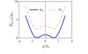
Figure 11: Dispersion curve of superfluid excitation energy for both branches at $T=0.05\mu_{S}$ and maximal superfluid polarization $h_{S}=h_{c}$. The solid line represents $E_{\alpha}$, and the dashed line represents $E_{\beta}$. The energy and the wavevector are normalized by $\mu_{S}$ and $k_{s}$, respectively, with $k_{s}=2m\mu_{S}/\hbar^{2}$ and $\mu_{S}$ the average chemical potential (7).

Figure 11 shows the superfluid dispersion relations for $E_{\alpha(\beta)}$ versus $q_{\alpha(\beta)}$, normalized by $\mu_{S}$ and $k_{s}$ respectively. At a given energy $E_{\alpha}$ there are up to two solutions for the magnitude of the wavevector of an $\alpha$ branch excitation, obtained from inverting Eqn. (17). Likewise, the wavevectors for the $\beta$ branch are obtained from inverting Eqn. (18).

In the normal phase, the wavevector solutions in the $\alpha$ branch are:

$$k_{p\uparrow}=\sqrt{\frac{2m}{\hbar^{2}}\left(\mu_{S\uparrow}-U_{N\uparrow}+E_{\alpha}-\xi_{\perp}\right)}$$ (62)

$$k_{h\downarrow}=\sqrt{\frac{2m^{*}}{\hbar^{2}}\left(\mu_{S\downarrow}-U_{N\downarrow}-E_{\alpha}\right)-\frac{2m}{\hbar^{2}}\xi_{\perp}}$$ (63)

In the superfluid phase, the wavevectors are:

$$q_{p\alpha}=\sqrt{\frac{2m}{\hbar^{2}}\left(\mu_{S}-U_{S}+\sqrt{\left(E_{\alpha}-U_{h}+h_{S}\right)^{2}-\Delta^{2}}-\xi_{\perp}\right)}$$ (64)

$$q_{h\alpha}=\sqrt{\frac{2m}{\hbar^{2}}\left(\mu_{S}-U_{S}-\sqrt{\left(E_{\alpha}-U_{h}+h_{S}\right)^{2}-\Delta^{2}}-\xi_{\perp}\right)}$$ (65)

For sufficiently large $E_{\alpha}$, the quantities inside the square roots of Eqns. (63) and (65) become negative, causing the hole wavevectors to become imaginary and give a vanishing current.

Appendix C Non-equilibrium distribution functions

Here we give the quasiparticle distribution functions $f_{n\alpha}$ and $f_{n\beta}$ for each channel. Using $f(E)=1/(1+e^{\beta E})$, $\delta\mu_{\uparrow}=\mu_{N\uparrow}-\mu_{S\uparrow}$, and $\delta\mu_{\downarrow}=\mu_{S\downarrow}-\mu_{N\downarrow}$, the $\alpha$ branch occupation numbers are:

$$f_{Lp\alpha}(E_{\alpha}) =f(E_{\alpha}-\delta\mu_{\uparrow})$$ (66)

$$f_{Lh\alpha}(E_{\alpha}) =f(E_{\alpha}-\delta\mu_{\downarrow})$$ (67)

$$f_{Rp\alpha}(E_{\alpha}) =f_{Rh\alpha}(E_{\alpha})=f(E_{\alpha})$$ (68)

The subtraction of $\delta\mu_{\sigma}$ in Eqns. (66) and (67) results from defining $E_{\alpha}$ relative to the superfluid chemical potentials $\mu_{S\sigma}$ for the purpose of the scattering calculation Blonder et al. (1982). For the $\beta$ branch:

$$f_{Lp\beta}(E_{\beta}) =f(E_{\beta}+\delta\mu_{\downarrow})$$ (69)

$$f_{Lh\beta}(E_{\beta}) =f(E_{\beta}+\delta\mu_{\uparrow})$$ (70)

$$f_{Rp\beta}(E_{\beta}) =f_{Rh\beta}(E_{\beta})=f(E_{\beta})$$ (71)

Appendix D Scattering regimes

Excitation (wavevector)	Accessible $E_{\alpha}$	Accessible $\xi_{\perp}$ (given $E_{\alpha}$)
Particle ($k_{p\uparrow}$)	$[0,\infty)$	$[0,\mu_{S\uparrow}-U_{N\uparrow}+E_{\alpha}]$
Hole ($k_{h\downarrow}$)	$[0,\mu_{S\downarrow}-U_{N\downarrow}]$	$[0,\frac{m^{*}}{m}(\mu_{S\downarrow}-U_{N\downarrow}-E_{\alpha})]$
Quasiparticle ($q_{p\alpha}$)	$[U_{h}-h_{S}+\Delta,\infty)$	$[0,\mu_{S}-U_{S}+\sqrt{(E_{\alpha}+h_{S}-U_{h})^{2}-\Delta^{2}}]$
Quasihole ($q_{h\alpha}$)	$[U_{h}-h_{S}+\Delta,U_{h}-h_{S}+\sqrt{(U_{S}-\mu_{S})^{2}+\Delta^{2}}]$	$[0,\mu_{S}-U_{S}-\sqrt{(E_{\alpha}+h_{S}-U_{h})^{2}-\Delta^{2}}]$
Equation (17) requires $E_{\alpha}\geq U_{h}-h_{S}$

Table 1: Conditions on $E_{\alpha}$ and $\xi_{\perp}$ that determine the scattering regimes for the $\alpha$ branch.

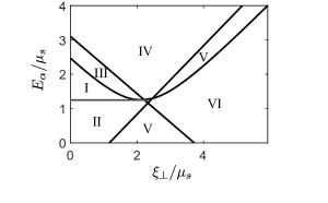
Figure 12: Alpha branch scattering regimes on the excitation energy $E_{\alpha}$ vs transverse kinetic energy $\xi_{\perp}$ plane. The case shown has $\mu_{N}=\mu_{S}$ and $p_{N}=0.8$. The other parameters, normalized by $\mu_{S}$, are $T=0.05$, $h_{S}=0$, $U_{S}=1.13$, $U_{h}=0$, $U_{N\uparrow}=0.16$, $U_{N\downarrow}=2.10$.

For a given excitation energy $E_{\alpha}$ and transverse momentum $k_{\perp}$, each of the four types of $\alpha$-branch excitations can be either allowed (real wavevector) or forbidden (imaginary wavevector), leading to different scattering regimes. Table 1 lists the conditions on each type of excitation. An example of the scattering regimes is shown in Fig. 12 on the plane of excitation energy vs $\xi_{\perp}\equiv\hbar^{2}k_{\perp}^{2}/(2m)$. In Regime I, all four excitation types are allowed. Regime II supports only normal particle and hole modes and therefore only allows transmission by Andreev reflection. Regime III allows the particle, quasiparticle and quasihole modes, and prohibits any transmission requiring the hole mode. Regime IV allows only the particle and quasiparticle modes and supports only the transmission between a particle and a quasiparticle. Regime V allows only the particle mode and, therefore, causes total reflection. Regime VI is the energetically forbidden regime, where the transverse kinetic energy exceeds the total kinetic energy. Since the Andreev current is important for the net current contribution, we present the formula for the Regime II:

$$j_{II,\alpha}^{Net}=\frac{2}{h}\,|r_{hp_{\alpha}}^{A}|^{2}\,[f(E_{\alpha}-\delta\mu_{\uparrow})-f(E_{\alpha}-\delta\mu_{\downarrow})]$$ (72)

The prefactor of 2 is typical for Andreev current and indicates the transport of two fermions per scattering event.

Appendix E Scattering coefficients

The scattering coefficients necessary for the determination of the currents are:

$$r_{pp_{\alpha}}^{A}= \frac{1}{c_{0}}\left[u_{0}^{2}\left(k_{p\uparrow}-q_{p\alpha}-ik_{\Lambda}\right)\left(\frac{m}{m^{*}}k_{h\downarrow}+q_{h\alpha}-ik_{\Lambda}\right)\right.$$

$$+\left.v_{0}^{2}\left(q_{p\alpha}-\frac{m}{m^{*}}k_{h\downarrow}+ik_{\Lambda}\right)\left(k_{p\uparrow}+q_{h\alpha}-ik_{\Lambda}\right)\right]$$ (73)

$$r_{hp_{\alpha}}^{A}= \frac{1}{c_{0}}2u_{0}v_{0}\sqrt{\frac{m}{m^{*}}k_{h\downarrow}k_{p\uparrow}}\,\left(q_{h\alpha}+q_{p\alpha}\right)e^{-iX_{0}}$$ (74)

$$r_{hh_{\alpha}}^{B}= \frac{1}{c_{0}}\left[u_{0}^{2}\left(\frac{m}{m^{*}}k_{h\downarrow}-q_{h\alpha}+ik_{\Lambda}\right)\left(q_{p\alpha}+k_{p\uparrow}+ik_{\Lambda}\right)\right.$$

$$\left.+v_{0}^{2}\left(q_{h\alpha}-k_{p\uparrow}-ik_{\Lambda}\right)\left(q_{p\alpha}+\frac{m}{m^{*}}k_{h\downarrow}+ik_{\Lambda}\right)\right]$$ (75)

where

$$c_{0}= u_{0}^{2}\left(k_{p\uparrow}+q_{p\alpha}+ik_{\Lambda}\right)\left(\frac{m}{m^{*}}k_{h\downarrow}+q_{h\alpha}-ik_{\Lambda}\right)$$

$$+v_{0}^{2}\left(q_{e}-\frac{m}{m^{*}}k_{h\downarrow}+ik_{\Lambda}\right)\left(k_{p\uparrow}-q_{h\alpha}+ik_{\Lambda}\right)$$ (76)

and $X_{0}$ denotes the phase of the gap $\Delta=|\Delta|e^{iX_{0}}$. We set $X_{0}=0$ without loss of generality. The transmission coefficients for channel A are:

$$t_{pp_{\alpha}}^{A}=\frac{1}{c_{0}}2u_{0}\sqrt{q_{p\alpha}k_{p\uparrow}}\,\left(q_{h\alpha}+\frac{m}{m^{*}}k_{h\downarrow}-ik_{\Lambda}\right)\sqrt{\frac{\xi_{s}}{E_{s}}}e^{-iX_{0}/2}$$ (77)

$$t_{hp_{\alpha}}^{A}=\frac{1}{c_{0}}2v_{0}\sqrt{k_{p\uparrow}q_{h\alpha}}\,\left(q_{p\alpha}-\frac{m}{m^{*}}k_{h\downarrow}+ik_{\Lambda}\right)\sqrt{\frac{\xi_{s}}{E_{s}}}e^{-iX_{0}/2}$$ (78)

And for channel B:

$$t_{ph_{\alpha}}^{B}=\frac{1}{c_{0}}2v_{0}\sqrt{\frac{m}{m^{*}}k_{h\downarrow}q_{e\alpha}}\,\left(q_{h\alpha}-k_{e\uparrow}-ik_{\Lambda}\right)\sqrt{\frac{\xi_{s}}{E_{s}}}e^{iX_{0}/2}$$ (79)

$$t_{hh_{\alpha}}^{B}=\frac{1}{c_{0}}2u_{0}\sqrt{\frac{m}{m^{*}}k_{h\downarrow}q_{h\alpha}}\,\left(q_{e\alpha}+k_{e\uparrow}+ik_{\Lambda}\right)\sqrt{\frac{\xi_{s}}{E_{s}}}e^{iX_{0}/2}$$ (80)

With the 7 coefficients given above, the other 9 coefficients for the $\alpha$ branch can be inferred from the symmetries of $S$-matrix.

Appendix F Additional Plots

We show an example of the dependence of the spin current on temperature in Fig. 13.

Figure 13: Spin current $J^{\text{spin}}/J_{0}$ plotted vs temperature $T/\mu_{S}\,$ under mechanical equilibrium with $p_{N}=99\%$, $h_{S}=0$.

Figure 14: Normalized chemical potential differences $\delta\mu_{\uparrow(\downarrow)}$ plotted vs $h_{N}$ under mechanical equilibrium, at $T=0.05\mu_{S}$, for (a) $h_{s}=0$ and (b) $h_{s}=h_{c}$. The dashed line shows the minimum of the superfluid excitation spectrum at the given value of $h_{s}$.

In Fig. 14, we show the chemical potential differences between the normal and superfluid regions versus the normal-region Zeeman field $h_{N}$ under mechanical equilibrium.

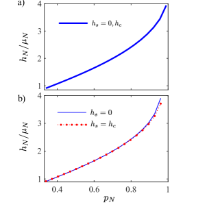
Figure 15: Zeeman field $h_{N}$ versus normal region polarization $p_{N}$ under the conditions (a) $\mu_{N}=\mu_{S}$, and (b) mechanical equilibrium. In case (a), $h_{N}/\mu_{S}$ is independent of $h_{S}$ because $\mu_{N}/\mu_{S}$ is constant.

Figure 15 shows the conversion between polarization and Zeeman field for the normal phase. In Fig. 15(b), the superfluid polarization leads to a slightly different conversion because the normal phase reacts to the increase in superfluid pressure at higher polarization.

References

- Shin et al. (2008) Yong-il Shin, Christian H. Schunck, André Schirotzek, and Wolfgang Ketterle, “Phase diagram of a two-component Fermi gas with resonant interactions,” Nature 451, 689 (2008).
- Navon et al. (2010) N. Navon, S. Nascimbène, F. Chevy, and C. Salomon, “The Equation of State of a Low-Temperature Fermi Gas with Tunable Interactions,” Science 328, 729–732 (2010).
- Nascimbène et al. (2010) S. Nascimbène, N. Navon, K. J. Jiang, F. Chevy, and C. Salomon, “Exploring the thermodynamics of a universal Fermi gas,” Nature 463, 1057 (2010).
- Nascimbène et al. (2011) S. Nascimbène, N. Navon, S. Pilati, F. Chevy, S. Giorgini, A. Georges, and C. Salomon, “Fermi-Liquid Behavior of the Normal Phase of a Strongly Interacting Gas of Cold Atoms,” Phys. Rev. Lett. 106, 215303 (2011).
- Ku et al. (2012) M. J. H. Ku, A. T. Sommer, L. W. Cheuk, and M. W. Zwierlein, “Revealing the Superfluid Lambda Transition in the Universal Thermodynamics of a Unitary Fermi Gas,” Science 335, 563–567 (2012).
- Van Houcke et al. (2012) K. Van Houcke, F. Werner, E. Kozik, N. Prokof’ev, B. Svistunov, M. J. H. Ku, A. T. Sommer, L. W. Cheuk, A. Schirotzek, and M. W. Zwierlein, “Feynman diagrams versus Fermi-gas Feynman emulator,” Nature Physics 8, 366–370 (2012).
- Schirotzek et al. (2008) André Schirotzek, Yong-il Shin, Christian H. Schunck, and Wolfgang Ketterle, “Determination of the Superfluid Gap in Atomic Fermi Gases by Quasiparticle Spectroscopy,” Phys. Rev. Lett. 101, 140403 (2008).
- Gaebler et al. (2010) J. P. Gaebler, J. T. Stewart, T. E. Drake, D. S. Jin, A. Perali, P. Pieri, and G. C. Strinati, “Observation of pseudogap behaviour in a strongly interacting Fermi gas,” Nature Physics 6, 569–573 (2010).
- Hoinka et al. (2017) Sascha Hoinka, Paul Dyke, Marcus G. Lingham, Jami J. Kinnunen, Georg M. Bruun, and Chris J. Vale, “Goldstone mode and pair-breaking excitations in atomic Fermi superfluids,” Nature Physics 13, 943–946 (2017).
- Sommer et al. (2011a) Ariel Sommer, Mark Ku, Giacomo Roati, and Martin W. Zwierlein, “Universal spin transport in a strongly interacting Fermi gas,” Nature 472, 201–204 (2011a).
- Sommer et al. (2011b) Ariel Sommer, Mark Ku, and Martin W Zwierlein, “Spin transport in polaronic and superfluid Fermi gases,” New Journal of Physics 13, 055009 (2011b).
- Cao et al. (2011) C. Cao, E. Elliott, J. Joseph, H. Wu, J. Petricka, T. Schäfer, and J. E. Thomas, “Universal Quantum Viscosity in a Unitary Fermi Gas,” Science 331, 58–61 (2011).
- Enss and Haussmann (2012) Tilman Enss and Rudolf Haussmann, “Quantum Mechanical Limitations to Spin Diffusion in the Unitary Fermi Gas,” Phys. Rev. Lett. 109, 195303 (2012).
- Valtolina et al. (2017) G. Valtolina, F. Scazza, A. Amico, A. Burchianti, A. Recati, T. Enss, M. Inguscio, M. Zaccanti, and G. Roati, “Exploring the ferromagnetic behaviour of a repulsive Fermi gas through spin dynamics,” Nature Physics 13, 704 (2017).
- Enss and Thywissen (2019) Tilman Enss and Joseph H. Thywissen, “Universal Spin Transport and Quantum Bounds for Unitary Fermions,” Annual Review of Condensed Matter Physics 10, 85–106 (2019).
- Tajima et al. (2020) Hiroyuki Tajima, Alessio Recati, and Yoji Ohashi, “Spin-dipole mode in a trapped Fermi gas near unitarity,” Phys. Rev. A 101, 013610 (2020).
- Brantut et al. (2012) Jean-Philippe Brantut, Jakob Meineke, David Stadler, Sebastian Krinner, and Tilman Esslinger, “Conduction of Ultracold Fermions Through a Mesoscopic Channel,” Science 337, 1069–1071 (2012).
- Husmann et al. (2015) Dominik Husmann, Shun Uchino, Sebastian Krinner, Martin Lebrat, Thierry Giamarchi, Tilman Esslinger, and Jean-Philippe Brantut, “Connecting strongly correlated superfluids by a quantum point contact,” Science 350, 1498–1501 (2015).
- Krinner et al. (2016) Sebastian Krinner, Martin Lebrat, Dominik Husmann, Charles Grenier, Jean-Philippe Brantut, and Tilman Esslinger, “Mapping out spin and particle conductances in a quantum point contact,” PNAS 113, 8144–8149 (2016).
- Kanász-Nagy et al. (2016) M. Kanász-Nagy, L. Glazman, T. Esslinger, and E. A. Demler, “Anomalous Conductances in an Ultracold Quantum Wire,” Phys. Rev. Lett. 117, 255302 (2016).
- Häusler et al. (2017) Samuel Häusler, Shuta Nakajima, Martin Lebrat, Dominik Husmann, Sebastian Krinner, Tilman Esslinger, and Jean-Philippe Brantut, “Scanning Gate Microscope for Cold Atomic Gases,” Phys. Rev. Lett. 119, 030403 (2017).
- Corman et al. (2019) Laura Corman, Philipp Fabritius, Samuel Häusler, Jeffrey Mohan, Lena H. Dogra, Dominik Husmann, Martin Lebrat, and Tilman Esslinger, “Quantized conductance through a dissipative atomic point contact,” Phys. Rev. A 100, 053605 (2019).
- Ono et al. (2021) Koki Ono, Toshiya Higomoto, Yugo Saito, Shun Uchino, Yusuke Nishida, and Yoshiro Takahashi, “Observation of spin-space quantum transport induced by an atomic quantum point contact,” Nat Commun 12, 6724 (2021).
- Valtolina et al. (2015) Giacomo Valtolina, Alessia Burchianti, Andrea Amico, Elettra Neri, Klejdja Xhani, Jorge Amin Seman, Andrea Trombettoni, Augusto Smerzi, Matteo Zaccanti, Massimo Inguscio, and Giacomo Roati, “Josephson effect in fermionic superfluids across the BEC-BCS crossover,” Science 350, 1505–1508 (2015).
- Burchianti et al. (2018) A. Burchianti, F. Scazza, A. Amico, G. Valtolina, J. A. Seman, C. Fort, M. Zaccanti, M. Inguscio, and G. Roati, “Connecting Dissipation and Phase Slips in a Josephson Junction between Fermionic Superfluids,” Phys. Rev. Lett. 120, 025302 (2018).
- Zaccanti and Zwerger (2019) M. Zaccanti and W. Zwerger, “Critical Josephson current in BCS-BEC–crossover superfluids,” Phys. Rev. A 100, 063601 (2019).
- Luick et al. (2020) Niclas Luick, Lennart Sobirey, Markus Bohlen, Vijay Pal Singh, Ludwig Mathey, Thomas Lompe, and Henning Moritz, “An ideal Josephson junction in an ultracold two-dimensional Fermi gas,” Science 369, 89–91 (2020).
- Del Pace et al. (2021) G. Del Pace, W. J. Kwon, M. Zaccanti, G. Roati, and F. Scazza, “Tunneling Transport of Unitary Fermions across the Superfluid Transition,” Phys. Rev. Lett. 126, 055301 (2021).
- Berggren et al. (2016) S. Berggren, B. J. Taylor, E. E. Mitchell, K. E. Hannam, J. Y. Lazar, and A. Leese De Escobar, “Computational Modeling of bi-Superconducting Quantum Interference Devices for High-Temperature Superconducting Prototype Chips,” IEEE Transactions on Applied Superconductivity 26, 1–6 (2016).
- Perconte et al. (2018) David Perconte, Fabian A. Cuellar, Constance Moreau-Luchaire, Maelis Piquemal-Banci, Regina Galceran, Piran R. Kidambi, Marie-Blandine Martin, Stephan Hofmann, Rozenn Bernard, Bruno Dlubak, Pierre Seneor, and Javier E. Villegas, “Tunable Klein-like tunnelling of high-temperature superconducting pairs into graphene,” Nature Physics 14, 25–29 (2018).
- Visani et al. (2012) C. Visani, Z. Sefrioui, J. Tornos, C. Leon, J. Briatico, M. Bibes, A. Barthélémy, J. Santamaría, and Javier E. Villegas, “Equal-spin Andreev reflection and long-range coherent transport in high-temperature superconductor/half-metallic ferromagnet junctions,” Nature Phys 8, 539–543 (2012).
- Komori et al. (2018) S. Komori, A. Di Bernardo, A. I. Buzdin, M. G. Blamire, and J. W. A. Robinson, “Magnetic Exchange Fields and Domain Wall Superconductivity at an All-Oxide Superconductor-Ferromagnet Insulator Interface,” Phys. Rev. Lett. 121, 077003 (2018).
- Bouscher et al. (2020) Shlomi Bouscher, Zhixin Kang, Krishna Balasubramanian, Dmitry Panna, Pu Yu, Xi Chen, and Alex Hayat, “High-Tc Cooper-pair injection in a semiconductor–superconductor structure,” J. Phys.: Condens. Matter 32, 475502 (2020).
- Bulgac and Forbes (2007) Aurel Bulgac and Michael McNeil Forbes, “Zero-temperature thermodynamics of asymmetric Fermi gases at unitarity,” Phys. Rev. A 75, 031605(R) (2007).
- Shin (2008) Yong-il Shin, “Determination of the equation of state of a polarized Fermi gas at unitarity,” Phys. Rev. A 77, 041603(R) (2008).
- Baur et al. (2009) Stefan K. Baur, Sourish Basu, Theja N. De Silva, and Erich J. Mueller, “Theory of the normal-superfluid interface in population-imbalanced Fermi gases,” Phys. Rev. A 79, 063628 (2009).
- Pilati and Giorgini (2008) S. Pilati and S. Giorgini, “Phase Separation in a Polarized Fermi Gas at Zero Temperature,” Phys. Rev. Lett. 100, 030401 (2008).
- Liu et al. (2008) Xia-Ji Liu, Hui Hu, and Peter D. Drummond, “Finite-temperature phase diagram of a spin-polarized ultracold Fermi gas in a highly elongated harmonic trap,” Phys. Rev. A 78, 023601 (2008).
- Olsen et al. (2015) Ben A. Olsen, Melissa C. Revelle, Jacob A. Fry, Daniel E. Sheehy, and Randall G. Hulet, “Phase diagram of a strongly interacting spin-imbalanced Fermi gas,” Phys. Rev. A 92, 063616 (2015).
- de Jong and Beenakker (1995) M. J. M. de Jong and C. W. J. Beenakker, “Andreev Reflection in Ferromagnet-Superconductor Junctions,” Phys. Rev. Lett. 74, 1657–1660 (1995).
- Halterman and Valls (2004) Klaus Halterman and Oriol T. Valls, “Layered ferromagnet-superconductor structures: The state and proximity effects,” Phys. Rev. B 69, 014517 (2004).
- Kashimura et al. (2010) Takashi Kashimura, Shunji Tsuchiya, and Yoji Ohashi, “Superfluid-ferromagnet-superfluid junction and the phase in a superfluid Fermi gas,” Phys. Rev. A 82, 033617 (2010).
- Alidoust and Halterman (2018) Mohammad Alidoust and Klaus Halterman, “Half-metallic superconducting triplet spin multivalves,” Phys. Rev. B 97, 064517 (2018).
- Van Schaeybroeck and Lazarides (2007) Bert Van Schaeybroeck and Achilleas Lazarides, “Normal-Superfluid Interface Scattering for Polarized Fermion Gases,” Phys. Rev. Lett. 98, 170402 (2007).
- Van Schaeybroeck and Lazarides (2009) Bert Van Schaeybroeck and Achilleas Lazarides, “Normal-superfluid interface for polarized fermion gases,” Phys. Rev. A 79, 053612 (2009).
- Parish and Huse (2009) Meera M. Parish and David A. Huse, “Evaporative depolarization and spin transport in a unitary trapped Fermi gas,” Phys. Rev. A 80, 063605 (2009).
- Liao et al. (2011) Y. A. Liao, M. Revelle, T. Paprotta, A. S. C. Rittner, Wenhui Li, G. B. Partridge, and R. G. Hulet, “Metastability in Spin-Polarized Fermi Gases,” Phys. Rev. Lett. 107, 145305 (2011).
- Magierski et al. (2019) Piotr Magierski, Buğra Tüzemen, and Gabriel Wlazłowski, “Spin-polarized droplets in the unitary Fermi gas,” Phys. Rev. A 100, 033613 (2019).
- Blonder et al. (1982) G. E. Blonder, M. Tinkham, and T. M. Klapwijk, “Transition from metallic to tunneling regimes in superconducting microconstrictions: Excess current, charge imbalance, and supercurrent conversion,” Phys. Rev. B 25, 4515–4532 (1982).
- Fischer et al. (2007) Øystein Fischer, Martin Kugler, Ivan Maggio-Aprile, Christophe Berthod, and Christoph Renner, “Scanning tunneling spectroscopy of high-temperature superconductors,” Rev. Mod. Phys. 79, 353–419 (2007).
- Mukherjee et al. (2017) Biswaroop Mukherjee, Zhenjie Yan, Parth B. Patel, Zoran Hadzibabic, Tarik Yefsah, Julian Struck, and Martin W. Zwierlein, “Homogeneous Atomic Fermi Gases,” Phys. Rev. Lett. 118, 123401 (2017).
- Gubbels and Stoof (2008) K. B. Gubbels and H. T. C. Stoof, “Renormalization Group Theory for the Imbalanced Fermi Gas,” Phys. Rev. Lett. 100, 140407 (2008).
- Gubbels and Stoof (2013) K. B. Gubbels and H. T. C. Stoof, “Imbalanced Fermi gases at unitarity,” Physics Reports 525, 255–313 (2013).
- Sheehy and Radzihovsky (2006) Daniel E. Sheehy and Leo Radzihovsky, “BEC-BCS Crossover in “Magnetized” Feshbach-Resonantly Paired Superfluids,” Phys. Rev. Lett. 96, 060401 (2006).
- Son and Stephanov (2006) D. T. Son and M. A. Stephanov, “Phase diagram of a cold polarized Fermi gas,” Phys. Rev. A 74, 013614 (2006).
- Yoshida and Yip (2007) Nobukatsu Yoshida and S.-K. Yip, “Larkin-Ovchinnikov state in resonant Fermi gas,” Phys. Rev. A 75, 063601 (2007).
- Parish et al. (2007) M. M. Parish, F. M. Marchetti, A. Lamacraft, and B. D. Simons, “Finite-temperature phase diagram of a polarized Fermi condensate,” Nature Phys 3, 124–128 (2007).
- Jensen et al. (2007) L. M. Jensen, J. Kinnunen, and P. Törmä, “Non-BCS superfluidity in trapped ultracold Fermi gases,” Phys. Rev. A 76, 033620 (2007).
- Kinnunen et al. (2018) Jami J Kinnunen, Jildou E Baarsma, Jani-Petri Martikainen, and Päivi Törmä, “The Fulde–Ferrell–Larkin–Ovchinnikov state for ultracold fermions in lattice and harmonic potentials: a review,” Rep. Prog. Phys. 81, 046401 (2018).
- Bulgac et al. (2006) Aurel Bulgac, Michael McNeil Forbes, and Achim Schwenk, “Induced -Wave Superfluidity in Asymmetric Fermi Gases,” Phys. Rev. Lett. 97, 020402 (2006).
- Bulgac and Yoon (2009) Aurel Bulgac and Sukjin Yoon, “Induced -wave superfluidity within the full energy- and momentum-dependent Eliashberg approximation in asymmetric dilute Fermi gases,” Phys. Rev. A 79, 053625 (2009).
- Patton and Sheehy (2012) Kelly R. Patton and Daniel E. Sheehy, “Induced superfluidity of imbalanced Fermi gases near unitarity,” Phys. Rev. A 85, 063625 (2012).
- Chaikin and Lubensky (1995) P. M. Chaikin and T. C. Lubensky, Principles of Condensed Matter Physics (Cambridge, 1995).
- Cetoli et al. (2013) A. Cetoli, J. Brand, R. G. Scott, F. Dalfovo, and L. P. Pitaevskii, “Snake instability of dark solitons in fermionic superfluids,” Phys. Rev. A 88, 043639 (2013).
- Wen et al. (2013) Wen Wen, Changqing Zhao, and Xiaodong Ma, “Dark-soliton dynamics and snake instability in superfluid Fermi gases trapped by an anisotropic harmonic potential,” Phys. Rev. A 88, 063621 (2013).
- Scherpelz et al. (2014) Peter Scherpelz, Karmela Padavić, Adam Rançon, Andreas Glatz, Igor S. Aranson, and K. Levin, “Phase Imprinting in Equilibrating Fermi Gases: The Transience of Vortex Rings and Other Defects,” Phys. Rev. Lett. 113, 125301 (2014).
- Ku et al. (2016) Mark J. H. Ku, Biswaroop Mukherjee, Tarik Yefsah, and Martin W. Zwierlein, “Cascade of Solitonic Excitations in a Superfluid Fermi gas: From Planar Solitons to Vortex Rings and Lines,” Phys. Rev. Lett. 116, 045304 (2016).
- Reichl and Mueller (2017) Matthew D. Reichl and Erich J. Mueller, “Core filling and snaking instability of dark solitons in spin-imbalanced superfluid Fermi gases,” Phys. Rev. A 95, 053637 (2017).
- Wlazłowski et al. (2018) Gabriel Wlazłowski, Kazuyuki Sekizawa, Maciej Marchwiany, and Piotr Magierski, “Suppressed Solitonic Cascade in Spin-Imbalanced Superfluid Fermi Gas,” Phys. Rev. Lett. 120, 253002 (2018).
- Tanaka and Kashiwaya (1995) Yukio Tanaka and Satoshi Kashiwaya, “Theory of Tunneling Spectroscopy of -Wave Superconductors,” Phys. Rev. Lett. 74, 3451–3454 (1995).
- Zürn et al. (2013) G. Zürn, T. Lompe, A. N. Wenz, S. Jochim, P. S. Julienne, and J. M. Hutson, “Precise Characterization of 6Li Feshbach Resonances Using Trap-Sideband-Resolved RF Spectroscopy of Weakly Bound Molecules,” Phys. Rev. Lett. 110, 135301 (2013).
- Yan et al. (2019) Zhenjie Yan, Parth B. Patel, Biswaroop Mukherjee, Richard J. Fletcher, Julian Struck, and Martin W. Zwierlein, “Boiling a Unitary Fermi Liquid,” Phys. Rev. Lett. 122, 093401 (2019).
- Combescot and Giraud (2008) R. Combescot and S. Giraud, “Normal State of Highly Polarized Fermi Gases: Full Many-Body Treatment,” Phys. Rev. Lett. 101, 050404 (2008).
- Prokof’ev and Svistunov (2008) Nikolay Prokof’ev and Boris Svistunov, “Fermi-polaron problem: Diagrammatic Monte Carlo method for divergent sign-alternating series,” Phys. Rev. B 77, 020408(R) (2008).
- Mora and Chevy (2010) Christophe Mora and Frédéric Chevy, “Normal Phase of an Imbalanced Fermi Gas,” Phys. Rev. Lett. 104, 230402 (2010).
- Bulgac and Forbes (2011) Aurel Bulgac and Michael McNeil Forbes, “Time-Dependent Superfluid Local-Density Approximation,” in Quantum Gases, Cold Atoms, Vol. 1 (Imperial College, 2011) pp. 397–406.
- Forbes et al. (2011) Michael McNeil Forbes, Stefano Gandolfi, and Alexandros Gezerlis, “Resonantly Interacting Fermions in a Box,” Phys. Rev. Lett. 106, 235303 (2011).
- Bulgac et al. (2012) Aurel Bulgac, Michael McNeil Forbes, and Piotr Magierski, “The Unitary Fermi Gas: From Monte Carlo to Density Functionals,” in The BCS-BEC Crossover and the Unitary Fermi Gas, Lecture Notes in Physics, edited by Wilhelm Zwerger (Springer, Berlin, Heidelberg, 2012) pp. 305–373.
- Bulgac (2013) Aurel Bulgac, “Time-Dependent Density Functional Theory and the Real-Time Dynamics of Fermi Superfluids,” Annual Review of Nuclear and Particle Science 63, 97–121 (2013).
- Kopyciński et al. (2021) Jakub Kopyciński, Wojciech R. Pudelko, and Gabriel Wlazłowski, “Vortex lattice in spin-imbalanced unitary Fermi gas,” Phys. Rev. A 104, 053322 (2021).
- Hossain et al. (2022) Khalid Hossain, Konrad Kobuszewski, Michael McNeil Forbes, Piotr Magierski, Kazuyuki Sekizawa, and Gabriel Wlazłowski, “Rotating quantum turbulence in the unitary Fermi gas,” Phys. Rev. A 105, 013304 (2022).
- Kawamura et al. (2020) Taira Kawamura, Ryo Hanai, Daichi Kagamihara, Daisuke Inotani, and Yoji Ohashi, “Nonequilibrium strong-coupling theory for a driven-dissipative ultracold Fermi gas in the BCS-BEC crossover region,” Phys. Rev. A 101, 013602 (2020).
- Wang et al. (2014) Jian-Sheng Wang, Bijay Kumar Agarwalla, Huanan Li, and Juzar Thingna, “Nonequilibrium Green’s function method for quantum thermal transport,” Front. Phys. 9, 673–697 (2014).
- Liu et al. (2017) Boyang Liu, Hui Zhai, and Shizhong Zhang, “Anomalous conductance of a strongly interacting Fermi gas through a quantum point contact,” Phys. Rev. A 95, 013623 (2017).
- Wlazłowski et al. (2013) Gabriel Wlazłowski, Piotr Magierski, Joaquín E. Drut, Aurel Bulgac, and Kenneth J. Roche, “Cooper Pairing Above the Critical Temperature in a Unitary Fermi Gas,” Phys. Rev. Lett. 110, 090401 (2013).
- Sekino et al. (2020) Yuta Sekino, Hiroyuki Tajima, and Shun Uchino, “Mesoscopic spin transport between strongly interacting Fermi gases,” Phys. Rev. Research 2, 023152 (2020).
- Frank et al. (2020) Bernhard Frank, Wilhelm Zwerger, and Tilman Enss, “Quantum critical thermal transport in the unitary Fermi gas,” Phys. Rev. Research 2, 023301 (2020).
- Carlson and Reddy (2005) J. Carlson and Sanjay Reddy, “Asymmetric Two-Component Fermion Systems in Strong Coupling,” Phys. Rev. Lett. 95, 060401 (2005).
- Magierski et al. (2009) Piotr Magierski, Gabriel Wlazłowski, Aurel Bulgac, and Joaquín E. Drut, “Finite-Temperature Pairing Gap of a Unitary Fermi Gas by Quantum Monte Carlo Calculations,” Phys. Rev. Lett. 103, 210403 (2009).
- Haussmann et al. (2009) R. Haussmann, M. Punk, and W. Zwerger, “Spectral functions and rf response of ultracold fermionic atoms,” Phys. Rev. A 80, 063612 (2009).
- Stewart et al. (2008) J. T. Stewart, J. P. Gaebler, and D. S. Jin, “Using photoemission spectroscopy to probe a strongly interacting Fermi gas,” Nature 454, 744–747 (2008).
- de Gennes (1989) P. G. de Gennes, Superconductivity of Metals and Alloys (Addison-Wesley, Redwood City, 1989).
- Haussmann et al. (2007) R. Haussmann, W. Rantner, S. Cerrito, and W. Zwerger, “Thermodynamics of the BCS-BEC crossover,” Phys. Rev. A 75, 023610 (2007).
- Mueller (2017) Erich J. Mueller, “Review of pseudogaps in strongly interacting Fermi gases,” Rep. Prog. Phys. 80, 104401 (2017).
- Mueller (2011) Erich J. Mueller, “Evolution of the pseudogap in a polarized Fermi gas,” Phys. Rev. A 83, 053623 (2011).
- BenDaniel and Duke (1966) D. J. BenDaniel and C. B. Duke, “Space-Charge Effects on Electron Tunneling,” Phys. Rev. 152, 683–692 (1966).
- Einevoll (1990) G. T. Einevoll, “Operator ordering in effective-mass theory for heterostructures. II. Strained systems,” Phys. Rev. B 42, 3497–3502 (1990).
- Cavalcante et al. (1997) F. S. A. Cavalcante, R. N. Costa Filho, J. Ribeiro Filho, C. A. S. de Almeida, and V. N. Freire, “Form of the quantum kinetic-energy operator with spatially varying effective mass,” Phys. Rev. B 55, 1326–1328 (1997).
- Srikanth and Raychaudhuri (1992) H. Srikanth and A.K. Raychaudhuri, “Modeling tunneling data of normal metal-oxide superconductor point contact junctions,” Physica C: Superconductivity 190, 229–233 (1992).
- Schirotzek et al. (2009) André Schirotzek, Cheng-Hsun Wu, Ariel Sommer, and Martin W. Zwierlein, “Observation of Fermi Polarons in a Tunable Fermi Liquid of Ultracold Atoms,” Phys. Rev. Lett. 102, 230402 (2009).
- Chevy (2006) F. Chevy, “Universal phase diagram of a strongly interacting Fermi gas with unbalanced spin populations,” Phys. Rev. A 74, 063628 (2006).