Normalizing Constant Estimation with Gaussianized Bridge Sampling

Abstract

Normalizing constant (also called partition function, Bayesian evidence, or marginal likelihood) is one of the central goals of Bayesian inference, yet most of the existing methods are both expensive and inaccurate. Here we develop a new approach, starting from posterior samples obtained with a standard Markov Chain Monte Carlo (MCMC). We apply a novel Normalizing Flow (NF) approach to obtain an analytic density estimator from these samples, followed by Optimal Bridge Sampling (OBS) to obtain the normalizing constant. We compare our method which we call Gaussianized Bridge Sampling (GBS) to existing methods such as Nested Sampling (NS) and Annealed Importance Sampling (AIS) on several examples, showing our method is both significantly faster and substantially more accurate than these methods, and comes with a reliable error estimation.

1 Introduction

Normalizing constant, also called partition function, Bayesian evidence, or marginal likelihood, is the central object of Bayesian methodology. Despite its importance, existing methods are both inaccurate and slow, and may require specialized tuning. One such method is Annealed Importance Sampling (AIS), and its alternative, Reverse AIS (RAIS), which can give stochastic lower and upper bounds to the normalizing constant, bracketing the true value (Neal, 2001; Grosse et al., 2015). However, as the tempered distribution may vary substantially with temperature, it can be expensive to obtain good samples at each temperature, which can lead to poor estimates (Murray et al., 2006). Nested sampling (NS) is another popular alternative (Skilling, 2004; Handley et al., 2015), which can be significantly more expensive than standard sampling methods in higher dimensions but, as we show, can also lead to very inaccurate estimates. Moreover, there is no simple way to know how accurate the estimate is.

Here we develop a new approach to the problem, combining Normalizing Flow (NF) density estimators with Optimal Bridge Sampling (OBS). In a typical Bayesian inference application, we first obtain posterior samples using one of the standard Markov Chain Monte Carlo (MCMC) methods. In our approach we use these samples to derive the normalizing constant with relatively few additional likelihood evaluations required, making the additional cost of normalizing constant estimation small compared to posterior sampling. All of our calculations are run on standard CPU platforms, and will be available in the BayesFast Python package.

2 Bridge Sampling

Let $p(\vec{x})$ and $q(\vec{x})$ be two possibly unnormalized distributions defined on $\Omega$, with normalizing constants $\mathcal{Z}_{p}$ and $\mathcal{Z}_{q}$. For any function $\alpha(\vec{x})$ on $\Omega$, we have

$$\int_{\Omega}\alpha(\vec{x})p(\vec{x})q(\vec{x})\text{d}\vec{x}=\mathcal{Z}_{p}\left<\alpha(\vec{x})q(\vec{x})\right>_{p}=\mathcal{Z}_{q}\left<\alpha(\vec{x})p(\vec{x})\right>_{q},$$ (1)

if the integral exists. Suppose that we have samples from both $p(\vec{x})$ and $q(\vec{x})$, and we know $\mathcal{Z}_{q}$, then eq:idendity gives

$$\mathcal{Z}_{p}=\frac{\left<\alpha(\vec{x})p(\vec{x})\right>_{q}}{\left<\alpha(\vec{x})q(\vec{x})\right>_{p}}\mathcal{Z}_{q},$$ (2)

which is the Bridge Sampling estimation of normalizing constant (Meng and Wong, 1996). It can be shown that many normalizing constant estimators, including Importance Sampling and Harmonic Mean, are special cases with different choices of bridge function $\alpha(\vec{x})$ (Gronau et al., 2017).

For a given proposal function $q(\vec{x})$, an asymptotically optimal bridge function can be constructed, such that the ratio $r=\mathcal{Z}_{p}/\mathcal{Z}_{q}$ is given by the root of the following score function equation

$$S(r)=\sum_{i=1}^{n_{p}}\frac{n_{q}rq(\vec{x}_{p,i})}{n_{p}p(\vec{x}_{p,i})+n_{q}rq(\vec{x}_{p,i})}-\sum_{i=1}^{n_{q}}\frac{n_{p}p(\vec{x}_{q,i})}{n_{p}p(\vec{x}_{q,i})+n_{q}rq(\vec{x}_{q,i})}=0,$$ (3)

where $n_{p}$ and $n_{q}$ are the numbers of samples from $p(\vec{x})$ and $q(\vec{x})$. For $r\geq 0$, $S(r)$ is monotonic and has a unique root, so one can easily solve it with e.g. secant method. This estimator is optimal, in the sense that its relative mean-square error is minimized (Chen et al., 2012).

Choosing a suitable proposal $q(\vec{x})$ for Bridge Sampling can be challenging, as it requires a large overlap between $q(\vec{x})$ and $p(\vec{x})$. One approach is Warp Bridge Sampling (WBS) (Meng and Schilling, 2002), which transforms $p(\vec{x})$ to a Gaussian with linear shifting, rescaling and symmetrizing. As we will show, this approach can be inaccurate or even fail completely for more complicated probability densities.

3 Normalizing Flow Based Density Estimation

As stated above, an appropriate proposal $q(\vec{x})$ which has large overlap with $p(\vec{x})$ is required for OBS to give accurate results. In a typical MCMC analysis we have samples from the posterior, so one can obtain an approximate density estimation $q(\vec{x})$ from these samples using a bijective NF. In this approach one maps $p(\vec{x})$ to an unstructured distribution such as zero mean unit variance Gaussian $\mathcal{N}(0,\vec{I})$. For density evaluation we must also keep track of the Jacobian of transformation $|\text{d}\vec{\Psi}/\text{d}\vec{x}|$, so that our estimated distribution is $q(\vec{x})=\mathcal{N}(0,\vec{I})|\text{d}\vec{\Psi}/\text{d}\vec{x}|$, where $\vec{\Psi}(\vec{x})$ is the transformation. The probability density $q(\vec{x})$ is normalized, so we know $\mathcal{Z}_{q}=1$. There have been various methods of NF recently proposed in machine learning literature (Dinh et al., 2014, 2016; Papamakarios et al., 2017), which however failed on several examples we present below. Moreover, we observed that training with these is very expensive and can easily dominate the overall computational cost.

For these reasons we instead develop Iterative Neural Transform (INT), a new NF approach, details of which will be presented elsewhere. It is based on combining optimal transport and information theory, repeatedly finding and transforming one dimensional marginals that are the most deviant between the target and proposal (Gaussian) distributions. After computing dual representation of Wasserstein-1 distance to find the maximally non-Gaussian directions, we apply a bijective transformation that maximizes the entropy along these directions. For this we use a non-parametric spline based transformation that matches the 1-d cumulative distribution function (CDF) of the data to a Gaussian CDF, where kernel density estimation (KDE) is used to smooth the probability density marginals. We found that using a fixed number of 5 to 10 iterations is sufficient for evidence estimation, and the computational cost of our NF density estimation is small when compared to the cost of sampling.

4 Proposed Method

We propose the following Gaussianized Bridge Sampling (GBS) approach, which combines OBS with NF density estimation. In our typical application, we first run No-U-Turn Sampler (NUTS) (Hoffman and Gelman, 2014) to obtain $2n_{p}$ samples from $p(\vec{x})$ if its gradient is available, while affine invariant sampling (Foreman-Mackey et al., 2013) can be used in the gradient-free case. To avoid underestimation of $\mathcal{Z}_{p}$ (Overstall and Forster, 2010), these $2n_{p}$ samples are divided into two batches, and we fit INT with the first batch of $n_{p}$ samples to obtain the proposal $q(\vec{x})$. Then we draw $n_{q}$ samples from $q(\vec{x})$ and evaluate their corresponding $p(\vec{x})$, where $n_{q}$ is determined by an adaptive rule (see apd:sbe). We solve for the normalizing constant ratio $r$ with eq:score, using these $n_{q}$ samples from $q(\vec{x})$ and the second batch of $n_{p}$ samples from $p(\vec{x})$ (also evaluating their corresponding $q(\vec{x})$), and report the result in form of $\ln\mathcal{Z}_{p}$, with its error approximated by the relative mean-square error of $\mathcal{Z}_{p}$ given in eq:error (Chen et al., 2012).

5 Examples

We used four test problems to compare the performance of various estimators. See apd:examples and B for more details of the examples and algorithms.

(1) The 16-d Funnel example is adapted from Neal et al. (2003). The funnel structure is common in Bayesian hierarchical models, and in practice it is recommended to reparameterize the model to overcome the pathology (Betancourt and Girolami, 2015). Here we stick to the original parameterization for test purpose.

(2) The 32-d Banana example comes from a popular variant of multidimensional Rosenbrock function (Rosenbrock, 1960), which is composed of 16 uncorrelated 2-d bananas. In addition, we apply a random 32-d rotation to the bananas, which makes all the parameters correlated with each other.

(3) The 48-d Cauchy example is adapted from the LogGamma example in Feroz et al. (2013); Buchner (2016). In contrast to the original example, where the mixture structure only exists in the first two dimensions, we place a mixture of two heavy-tailed Cauchy distributions along every dimension.

(4) The 64-d Ring example has strong non-linear correlation between the parameters, as the marginal distribution of every two successive parameters is ring-shaped.

fig:results , , ,

Figure 1: Comparison of normalizing constant estimators on the four examples, based on 64 simulations for each case. Note that some panels use symmetrical logarithmic scale for x-axis. See the main text for abbreviation keys. We show the quantiles of normalizing constant results on the left and the number of total evaluations on the right, separately for likelihood and its gradient. For WBS, GBS(L), GIS and GHM, the number of evaluations shown includes those required for posterior sampling, and the cost for evidence estimation alone is much smaller.

See fig:results for a comparison of the estimators. For all of the four test examples, the proposed GBS algorithm gives the most accurate result and a valid error estimation. We use NS as implemented in dynesty (Speagle, 2019) with its default settings. For all other cases, we use NUTS as the MCMC transition operator. We chose to run (R)AIS with equal number of evaluations as our GBS, but as seen from fig:results this number is inadequate for (R)AIS, which needs about 10-100 times more evaluations to achieve sufficient accuracy (see apd:ais). In contrast, if we run GBS with 4 times fewer evaluations (Gaussianized Bridge Sampling Lite, GBSL), we achieve an unbiased result with a larger error than GBS, but still smaller than other estimators. For comparison we also show results replacing OBS with IS (GIS) or HM (GHM), while still using INT for $q(\vec{x})$. Although GIS and GHM are better than NS or (R)AIS, they are worse than GBS(L), highlighting the importance of OBS. Finally, we also compare to WBS, which uses a very simple proposal distribution $q(\vec{x})$, and fails on several examples, highlighting the importance of using a more expressive NF for $q(\vec{x})$.

For our GBS(L), most of evaluation time is used to get the posterior samples with standard MCMC, which is a typical Bayesian inference goal, and the additional cost to evaluate evidence is small compared to the MCMC (see apd:sbe). In contrast, Thermodynamic Integration (TI) or (R)AIS is more expensive than posterior sampling, since the chains need to be accurate at every intermediate state (Neal, 1993). The same comment applies to NS, which is more expensive than the MCMC approaches we use here for posterior analysis, especially when non-informative prior is used.

6 Conclusion

We present a new method to estimate the normalizing constant (Bayesian evidence) in the context of Bayesian analysis. Our starting point are the samples from the posterior using standard MCMC based methods, and we assume that these have converged to the correct probability distribution. In our approach we combine OBS with INT, a novel NF based density estimator, showing on several high dimensional examples that our method outperforms other approaches in terms of accuracy and computational cost, and provides a reliable error estimate.

Appendix A Details of Examples

A.1 16-d Funnel

The model likelihood is

$$\mathcal{L}=\mathcal{N}(x_{1}\,|\,0,a^{2})\prod_{i=2}^{n}\mathcal{N}(x_{i}\,|\,0,\exp(2bx_{1})),\quad a=1,\quad b=0.5,\quad n=16,$$ (4)

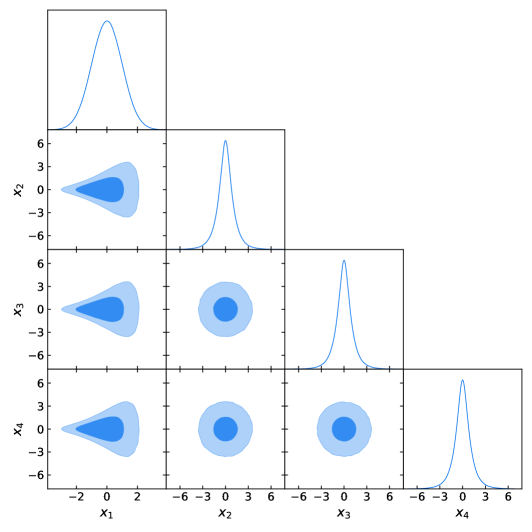
with flat prior $x_{1}\sim\mathcal{U}(-4,4)$, $x_{2:n}\sim\mathcal{U}(-30,30)$. We use $\ln\mathcal{Z}_{p}=-63.4988$ as the fiducial value, and the corner plot of the first four dimensions is shown in fig:funnel.

fig:funnel

Figure 2: Corner plot for the Funnel example.

A.2 32-d Banana

fig:banana

Figure 3: Corner plot for the Banana example. Top: without random rotation. Bottom: with random rotation.

The model likelihood is

$$\ln\mathcal{L}=-\sum_{i=1}^{n/2}\left[\,(y_{2i-1}^{2}-y_{2i})^{2}/Q+(y_{2i-1}-1)^{2}\,\right],\quad\vec{y}=\vec{A}\vec{x},\quad Q=0.01,\quad n=32,$$ (5)

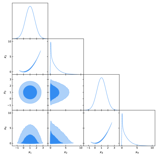
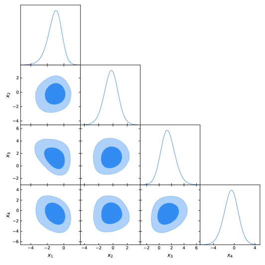
with flat prior $\mathcal{U}(-15,15)$ on all the parameters. The rotation matrix $\vec{A}$ is generated from a random sample of $\text{SO}(n)$, and the same $\vec{A}$ is used for all the simulations. We use $\ln\mathcal{Z}_{p}=-127.364$ as the fiducial value, and the corner plot of the first four dimensions, without or with the random rotation, is shown in fig:banana. The strong degeneracy can no longer be identified in the plot once we apply the rotation, however it still exists and hinders most estimators from getting reasonable results.

A.3 48-d Cauchy

The model likelihood is

$$\mathcal{L}=\prod_{i=1}^{n}\frac{1}{2}\left[\,\text{Cauchy}(x_{i}|\mu,\sigma)+\text{Cauchy}(x_{i}|{-\mu},\sigma)\,\right],\quad\mu=5,\quad\sigma=1,\quad n=48,$$ (6)

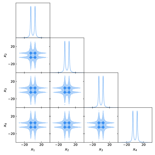
with flat prior $\mathcal{U}(-100,100)$ on all the parameters. We use $\ln\mathcal{Z}_{p}=-254.627$ as the fiducial value, and the corner plot of the first four dimensions is shown in fig:cauchy.

fig:cauchy

Figure 4: Corner plot for the Cauchy example.

A.4 64-d Ring

The model likelihood is

$$\ln\mathcal{L}=-\left[\frac{(x_{n}^{2}+x_{1}^{2}-a)^{2}}{b}\right]^{2}-\sum_{i=1}^{n-1}\left[\frac{(x_{i}^{2}+x_{i+1}^{2}-a)^{2}}{b}\right]^{2},\quad a=2,\quad b=1,\quad n=64,$$ (7)

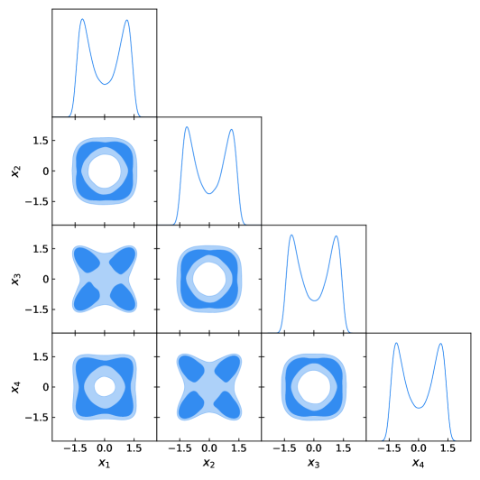
with flat prior $\mathcal{U}(-5,5)$ on all the parameters. We use $\ln\mathcal{Z}_{p}=-114.492$ as the fiducial value, and the corner plot of the first four dimensions is shown in fig:ring.

fig:ring

Figure 5: Corner plot for the Ring example.

Appendix B Details of Algorithms

B.1 Obtaining Fiducial Values

Analytic normalizing constants for the (unconstrained) likelihood of the Funnel, Banana and Cauchy examples are available. For the Funnel and Banana examples, we account for the effect of finite prior range by simply generating a large amount of samples and counting the fraction of the samples that are inside the prior range. For the Cauchy example, we directly evaluate its CDF. For the Ring example, the fiducial normalizing constant is obtained by a long AIS and RAIS run, with 300,000 intermediate states and 64 chains in both directions.

B.2 Nested Sampling

We use dynamic NS implemented in dynesty, which is considered more efficient than static NS. Traditionally, NS does not need the gradient of the likelihood, at the cost of lower sampling efficiency in high dimensions. Since analytic gradient of the four examples is available, we follow dynesty’s default setting, which requires the gradient to perform Hamitonian Slice Sampling for dimensions $d>20$. While for dimensions $10\leq d\leq 20$, random walks sampling is used instead. dynesty also provides an error estimate for the evidence; see Speagle (2019) for details.

B.3 (Reversed) Annealed Importance Sampling

For (R)AIS, we divide the warm-up iterations of NUTS into two equal stages, and the (flat) prior is used as the base density. In the first stage, we set $\beta=0.5$ and adapt the mass matrix and step size of NUTS, which acts as a compromise between the possibly broad prior and narrow posterior. In the second stage, we set $\beta=0$ ($\beta=1$) for AIS (RAIS) to get samples from the prior (posterior). After warm-up, we use the following sigmoidal schedule to perform annealing,

$$\tilde{\beta}_{t}=\sigma\left(\delta\left(\frac{2t}{T-1}-1\right)\right),\qquad\beta_{t}=\frac{\tilde{\beta}_{t}-\tilde{\beta}_{0}}{\tilde{\beta}_{T-1}-\tilde{\beta}_{0}},\qquad 0\leq t\leq T-1,$$ (8)

where $\sigma$ denotes the logistic sigmoid function and we set $\delta=4$ (Grosse et al., 2015). We use 1,000 warm-up iterations for all the four examples, and adjust the number of states $T$ so that it needs roughly the same number of evaluations as GBS in total. The exact numbers are listed in tab:ais. We run 16 chains for each case, and average reported $\ln\mathcal{Z}_{p}$ of different chains, which gives a stochastic lower (upper) bound for AIS (RAIS) according to Jensen’s inequality. The uncertainty is estimated from the scatter of different chains, and should be understood as the error of the lower (upper) bound of $\ln\mathcal{Z}_{p}$, instead of $\ln\mathcal{Z}_{p}$ itself.

tab:ais Funnel Banana Cauchy Ring AIS 800 2000 3000 3500 RAIS 700 1500 2500 3000

Table 1: The number of states $T$ used by (R)AIS.

Using the mass matrix and step size of NUTS adapted at $\beta=0.5$, and the prior as base density, may account for the phenomenon that RAIS failed to give an upper bound in the Banana example: the density is very broad at high temperatures and very narrow at low temperatures, which is difficult for samplers adapted at a single $\beta$. One may remedy this issue by using a better base density that is closer to the posterior, but this will require delicate hand-tuning and is beyond the scope of this paper. While the upper (lower) bounds of (R)AIS are valid in the limit of a very large number of samples, achieving this limit may be extremely costly in practice.

B.4 Sample-Based Estimators

The remaining normalizing constant estimators require a sufficient number of samples from $p(\vec{x})$, which we obtain with NUTS. For WBS, GBS, GIS and GHM, we run 8 chains with 2,500 iterations for the Funnel and Banana examples, and 5,000 iterations for the Cauchy and Ring examples, including the first 20% warm-up iterations, which are removed from the samples. Then we fit INT using 10 iterations for GBS, GIS and GHM, whose computation cost (a few seconds for the Funnel example) is small or negligible relative to NUTS sampling, and does not depend on the cost of $\ln p(\vec{x})$ evaluations. For GBSL, the number of NUTS chains, NUTS iterations and INT iterations are all reduced by half, leading to a factor of four decrease in the total computation cost.

The relative mean-square error of OBS is minimized and given by

$$\widehat{RE^{2}_{\text{OBS}}}=\frac{1}{n_{q}}\frac{\text{Var}_{q}(f_{1}(\vec{x}))}{\text{E}_{q}^{2}(f_{1}(\vec{x}))}+\frac{\tau_{f_{2}}}{n_{p}}\frac{\text{Var}_{p}(f_{2}(\vec{x}))}{\text{E}_{p}^{2}(f_{2}(\vec{x}))},$$ (9)

where $f_{1}(\vec{x})=\frac{p^{\prime}(\vec{x})}{s_{p}p^{\prime}(\vec{x})+s_{q}q(\vec{x})}$, $f_{2}(\vec{x})=\frac{q(\vec{x})}{s_{p}p^{\prime}(\vec{x})+s_{q}q(\vec{x})}$, $s_{p}=\frac{n_{p}}{n_{p}+n_{q}}$, $s_{q}=\frac{n_{q}}{n_{p}+n_{q}}$. Here $p^{\prime}(\vec{x})=p(\vec{x})/\mathcal{Z}_{p}$ and $q(\vec{x})$ should be normalized densities. We assume the samples from $q(\vec{x})$ are independent, whereas the samples from $p(\vec{x})$ may be autocorrelated, and $\tau_{f_{2}}$ is the integrated autocorrelation time of $f_{2}(\vec{x}_{p})$ (Frühwirth-Schnatter, 2004), which is estimated by the autocorr module in emcee (Foreman-Mackey et al., 2013). Analogous expressions can be derived for IS and HM,

$$\widehat{RE^{2}_{\text{IS}}}=\frac{1}{n_{q}}\text{Var}_{q}(f_{\text{IS}}(\vec{x})),\qquad f_{\text{IS}}(\vec{x})=\frac{p^{\prime}(\vec{x})}{q(\vec{x})},$$

$$\widehat{RE^{2}_{\text{HM}}}=\frac{\tau_{f_{\text{HM}}}}{n_{p}}\text{Var}_{p}(f_{\text{HM}}(\vec{x})),\qquad f_{\text{HM}}(\vec{x})=\frac{q(\vec{x})}{p^{\prime}(\vec{x})}.$$ (10)

The claimed uncertainty in fig:results is obtained by assuming that the error is Gaussian distributed.

There can be different strategies to allocate samples for BS. In the literature, it is recommended that one draws samples from $p(\vec{x})$ and $q(\vec{x})$ based on equal-sample-size or equal-time allocation (Bennett, 1976; Meng and Wong, 1996). Since NUTS based sampling usually requires at least hundreds of evaluations to obtain one effective sample from $p(\vec{x})$ in high dimensions (Hoffman and Gelman, 2014), which is orders of magnitude more expensive than our NF based sampling for $q(\vec{x})$, it could be advantageous to set $n_{q}>n_{p}$. Throughout this paper, the following adaptive strategy is adopted to determine $n_{q}$ for GBS(L). After obtaining $2n_{p}$ samples from $p(\vec{x})$, we divide them into two equal batches, which will be used for fitting the proposal $q(\vec{x})$ and evaluating the evidence, respectively. As an starting point, we draw $n_{q,0}=n_{p}$ samples from $q(\vec{x})$ and estimate the error of OBS using eq:error. Note that the right side of eq:error is composed of two terms, and only the first term will decrease as one increases $n_{q}$ but fixes $n_{p}$. Assuming that current samples provide an accurate estimate of the variance and expectation terms in eq:error, one can solve for $n_{q}$ such that $f_{\text{err}}$, the fraction of $q(\vec{x})$ contributions in eq:error, is equal to some specified value, which we set to 0.1. Since the $n_{q,0}$ samples from $q(\vec{x})$ can be reused, if $n_{q}<n_{q,0}$, no additional samples are required and we set $n_{q}=n_{q,0}$. On the other hand, we also require that $f_{\text{eva}}$, the fraction of $p(\vec{x})$ evaluations that are used for the $q(\vec{x})$ samples, is no larger than 0.1, although this constraint is usually not activated in practice.

We use 0.1 as the default values of $f_{\text{err}}$ and $f_{\text{eva}}$, so that the additional cost of evidence evaluation is small relative to the cost of sampling, while using a larger $n_{q}$ alone can no longer significantly improve the accuracy of normalizing constant. However, if one wants to put more emphasis on posterior sampling (evidence estimation), a larger (smaller) $f_{\text{err}}$ and/or smaller (larger) $f_{\text{eva}}$ can be used. In principle, it is also possible to use different number of $p(\vec{x})$ samples to fit the proposal and evaluate the evidence, in contrast to equal split used in Overstall and Forster (2010), which we leave for feature research.

For GIS and WBS, we use the same $n_{q}$ as solved for GBS(L). No samples from $p(\vec{x})$ are required to estimate normalizing constant for GIS, so in this case all the $2n_{p}$ samples will be used to fit INT. While for GHM, no samples from $q(\vec{x})$ are required. Note that for WBS, the additional $p(\vec{x})$ evaluations required for evidence estimation is $n_{p}+2n_{q}$ instead of $n_{q}$, which comes from the symmetrization of $\ln p(\vec{x})$.

References

- Bennett (1976) Charles H Bennett. Efficient estimation of free energy differences from monte carlo data. Journal of Computational Physics, 22(2):245–268, 1976.
- Betancourt and Girolami (2015) Michael Betancourt and Mark Girolami. Hamiltonian monte carlo for hierarchical models. Current trends in Bayesian methodology with applications, 79:30, 2015.
- Buchner (2016) Johannes Buchner. A statistical test for nested sampling algorithms. Statistics and Computing, 26(1-2):383–392, 2016.
- Chen et al. (2012) Ming-Hui Chen, Qi-Man Shao, and Joseph G Ibrahim. Monte Carlo methods in Bayesian computation. Springer Science & Business Media, 2012.
- Dinh et al. (2014) Laurent Dinh, David Krueger, and Yoshua Bengio. NICE: non-linear independent components estimation. CoRR, abs/1410.8516, 2014. URL http://arxiv.org/abs/1410.8516.
- Dinh et al. (2016) Laurent Dinh, Jascha Sohl-Dickstein, and Samy Bengio. Density estimation using real NVP. CoRR, abs/1605.08803, 2016. URL http://arxiv.org/abs/1605.08803.
- Feroz et al. (2013) F Feroz, MP Hobson, E Cameron, and AN Pettitt. Importance nested sampling and the multinest algorithm. arXiv preprint arXiv:1306.2144, 2013.
- Foreman-Mackey et al. (2013) Daniel Foreman-Mackey, David W Hogg, Dustin Lang, and Jonathan Goodman. emcee: the mcmc hammer. Publications of the Astronomical Society of the Pacific, 125(925):306, 2013.
- Frühwirth-Schnatter (2004) Sylvia Frühwirth-Schnatter. Estimating marginal likelihoods for mixture and markov switching models using bridge sampling techniques. The Econometrics Journal, 7(1):143–167, 2004.
- Gronau et al. (2017) Quentin F Gronau, Alexandra Sarafoglou, Dora Matzke, Alexander Ly, Udo Boehm, Maarten Marsman, David S Leslie, Jonathan J Forster, Eric-Jan Wagenmakers, and Helen Steingroever. A tutorial on bridge sampling. Journal of mathematical psychology, 81:80–97, 2017.
- Grosse et al. (2015) Roger B Grosse, Zoubin Ghahramani, and Ryan P Adams. Sandwiching the marginal likelihood using bidirectional monte carlo. arXiv preprint arXiv:1511.02543, 2015.
- Handley et al. (2015) W. J. Handley, M. P. Hobson, and A. N. Lasenby. POLYCHORD: next-generation nested sampling. MNRAS, 453:4384–4398, November 2015. 10.1093/mnras/stv1911.
- Hoffman and Gelman (2014) Matthew D Hoffman and Andrew Gelman. The no-u-turn sampler: adaptively setting path lengths in hamiltonian monte carlo. Journal of Machine Learning Research, 15(1):1593–1623, 2014.
- Meng and Schilling (2002) Xiao-Li Meng and Stephen Schilling. Warp bridge sampling. Journal of Computational and Graphical Statistics, 11(3):552–586, 2002.
- Meng and Wong (1996) Xiao-Li Meng and Wing Hung Wong. Simulating ratios of normalizing constants via a simple identity: a theoretical exploration. Statistica Sinica, pages 831–860, 1996.
- Murray et al. (2006) Iain Murray, David MacKay, Zoubin Ghahramani, and John Skilling. Nested sampling for potts models. In Advances in Neural Information Processing Systems, pages 947–954, 2006.
- Neal (1993) Radford M Neal. Probabilistic inference using Markov chain Monte Carlo methods. Department of Computer Science, University of Toronto Toronto, Ontario, Canada, 1993.
- Neal (2001) Radford M Neal. Annealed importance sampling. Statistics and computing, 11(2):125–139, 2001.
- Neal et al. (2003) Radford M Neal et al. Slice sampling. The annals of statistics, 31(3):705–767, 2003.
- Overstall and Forster (2010) Antony M Overstall and Jonathan J Forster. Default bayesian model determination methods for generalised linear mixed models. Computational Statistics & Data Analysis, 54(12):3269–3288, 2010.
- Papamakarios et al. (2017) George Papamakarios, Iain Murray, and Theo Pavlakou. Masked autoregressive flow for density estimation. In Advances in Neural Information Processing Systems 30: Annual Conference on Neural Information Processing Systems 2017, 4-9 December 2017, Long Beach, CA, USA, pages 2335–2344, 2017. URL http://papers.nips.cc/paper/6828-masked-autoregressive-flow-for-density-estimation.
- Rosenbrock (1960) HoHo Rosenbrock. An automatic method for finding the greatest or least value of a function. The Computer Journal, 3(3):175–184, 1960.
- Skilling (2004) John Skilling. Nested sampling. In AIP Conference Proceedings, volume 735, pages 395–405. AIP, 2004.
- Speagle (2019) Joshua S Speagle. dynesty: A dynamic nested sampling package for estimating bayesian posteriors and evidences. arXiv preprint arXiv:1904.02180, 2019.