Grid Search, Random Search, Genetic Algorithm: A Big Comparison for NAS

Abstract

In this paper, we compare the three most popular algorithms for hyperparameter optimization (Grid Search, Random Search, and Genetic Algorithm) and attempt to use them for neural architecture search (NAS). We use these algorithms for building a convolutional neural network (search architecture). Experimental results on CIFAR-10 dataset further demonstrate the performance difference between compared algorithms. The comparison results are based on the execution time of the above algorithms and accuracy of the proposed models.

Keywords: Neural architecture search, grid search, random search, genetic algorithm, hyperparameter optimization

1 Introduction

Over the last few years, convolutional neural networks (CNNs) and their varieties have seen great results on a variety of machine learning problems and applications (Shin et al. (2016); Krizhevsky et al. (2012); Wu (2019); Xu et al. (2014); Goodfellow et al. (2014)). However, each of the currently known architectures is designed by human experts in machine learning (Simonyan and Zisserman (2014); Szegedy et al. (2014); He et al. (2015a)). Today, the number of tasks that can be solved using neural networks is growing rapidly and designing a neural network architecture becomes a long, slow and expensive process. It’s a big challenge to design a good neural network.

Typical CNN architecture consists of several convolution, pooling, and fully-connected layers. While designing a network architecture, an expert has to make a lot of design choices: the number of layers of each type (convolution, pooling, dense, etc.), the ordering of the layers, the hyperparameters for each layer, the receptive field size, stride, padding for a convolution layer, etc.

Many kinds of research in the field of so-called automated machine learning (Auto-ML) have been made (Zhong et al. (2017); Cai et al. (2018)). Zoph and Le (2016) propose a reinforcement learning-based method for neural architecture search. Hebbal et al. (2019) experiment with Bayesian optimization algorithm using deep Gaussian processes. Pham et al. (2018) propose another approach using parameter sharing. Jin et al. (2018) and Weill et al. (2019) presented the most inspiring frameworks for NAS and Auto-ML called Auto Keras and AdaNet respectively.

Despite advances in the field of automated machine learning, in this paper, we attempt to use classic hyperparameter optimization algorithms to find the optimal neural network architecture. We compare the execution time between the above algorithms and finally will know what algorithm proposes a model with the highest score for less time.

2 Search space

The search space defines which neural network architectures might be discovered by used algorithm. There are many methods and strategies for neural architecture search of CNNs. In most cases, experts build architecture from scratch by alternating convolutional and fully-connected layers.

The simple search space is the space of chain-structured neural networks, as illustrated in Figure 1 (Elsken et al. (2018)).

Figure 1: An illustration of different architecture spaces. Each node in the graphs corresponds to a layer in a neural network: a convolutional or pooling layer, etc. An edge from layer ${L_{i}}$ to layer ${L_{j}}$ denotes that ${L_{j}}$ receives the output of ${L_{i}}$ as input. Left: an element of a chain-structured space. Right: an element of a more complex search space with additional layer types and multiple branches and skip connections (Elsken et al. (2018).)

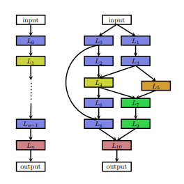
Rather than designing the entire convolutional network, one can design smaller modules and then connect them together to form a network (Pham et al. (2018)). Using this approach, a neural network architecture can be written as a sequence of layers. Then the search space is parametrized by:

• $n$ number of layers;

• type of every layer (e.g., convolutional, pooling, fully-connected layers);

• hyperparameters of every layer (e.g., kernel size and filters for a convolutional layer).

In this paper, we use the next approach:

1) Define our basic architecture, as illustrated in Figure 2.

Figure 2: An illustration of a basic CNN architecture. The search space defines the number of convolutional and dense blocks.

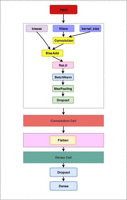
2) Build a new architecture by adding the convolutional and dense cells (Figure 3) to the basic architecture. A dense cell is just a fully-connected layer with ReLU activation.

Figure 3: An illustration of a convolutional block. This block accepts the following parameters as required: input, filters, kernel size. If additional parameters are specified, the output is passed through the BatchNormalization and MaxPooling layers.

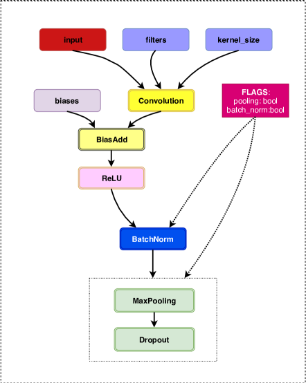
The choice of the search space determines the difficulty of the optimization problem: even for the case of the search space based on a single cell with fixed architecture, the optimization problem remains difficult (Elsken et al. (2018)) and relatively high-dimensional (since more complex models tend to perform better, resulting in more design choices).

3 Search strategy

Grid Search.

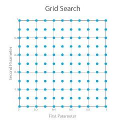
The traditional method of hyperparameters optimization is a grid search, which simply makes a complete search over a given subset of the hyperparameters space of the training algorithm (Figure 4). Because the machine learning algorithm parameter space may include spaces with real or unlimited values for some parameters, it is possible that we need to specify a boundary to apply a grid search. Grid search suffers from high dimensional spaces, but often can easily be parallelized, since the hyperparameter values that the algorithm works with are usually independent of each other.

Figure 4: An illustration of a grid search space. We manually set a range of the possible parameters and the algorithm makes a complete search over them. In other words, the grid search algorithm is a complete brute-force and takes a too long time to execute.

Random Search.

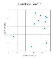
It overrides the complete selection of all combinations by their random selection. This can be easily applied to discrete cases, but the method can be generalized to continuous and mixed spaces. Random search can outperform a grid search, especially if only a small number of hyperparameters affect the performance of the machine learning algorithm.

Figure 5: An illustration of a random search space. We manually set a range of bounds of the possible parameters and the algorithm makes a search over them for the number of iterations we set.

Genetic Algorithm.

The genetic algorithm is an evolutionary search algorithm used to solve optimization and modeling problems by sequentially selecting, combining, and varying parameters using mechanisms that resemble biological evolution. Genetic algorithms simulate the process of natural selection which means those species who can adapt to changes in their environment can survive and reproduce and go to the next generation.

Each generation consist of a population of individuals and each individual represents a point in search space and possible solution. Each individual is represented as a string of character/integer/float/bits. This string is analogous to the chromosome.

The genetic algorithm begins with a randomly generated population of chromosomes. Then, it makes a selection process and recombination, based on each chromosome fitness (score). Parent genetic materials are recombined to generate child chromosomes producing the next generation. This process is iterated until some stopping criterion is reached (Loussaief and Abdelkrim (2018)).

4 Experiments and Results

Dataset.

In our experiments we use the CIFAR-10 dataset with data preprocessing and augmentation procedures. This dataset consists of 50,000 training images and 10,000 test images. We first preprocess the data by mean and standart deviation normalization. Additionally, we shift the training images horizontally and vertically, and randomly flipping them horizontally.

Search spaces.

We apply each of the algorithm to one search space: the macro search space over basic convolutional model with adding convolutional cells to it (Section 2).

Training details.

All convolutional kernels are initialized with He uniform initialization (He et al. (2015b)). We also apply $L_{2}$ weight decay with rate $10^{-4}$ and set the kernel size in convolutions to 3. The first convolutional layer uses 32 filters. Each convolutional cell uses 64 filters. All convolutions are followed by BatchNormalization with MaxPooling. The parameters of each network are trained with Adamax optimizer (Kingma and Ba (2014)), where the learning rate is set to $2e-3$ and other parameters is stay by default. We set the dropout rate to 0.2 in each convolutional cell. Dropout rate in the basic model is 0.5 and the number of units in the dense cells is 512. Each architecture search is run for 50 epochs on Nvidia Tesla K80 GPU. The basic model achieves 76% accuracy after 50 epochs.

4.1 Grid Search

The possible number of the convolutional cells is set to (0, 2, 3, 4) and number of the dense cells is set to (1, 2).

Results.

The whole trainig procedure of $2\times 4=8$ (length of conv cells list $\times$ length of dence cells list) models took $\approx$4.3 hours.

Model params			Evaluating
Conv cells	Dense cells	Size	Accuracy %	Score
0	1	4.2M	75$\pm$0.3	0.72
0	2	4.4M	77$\pm$0.2	0.74
2	1	0.58M	82	0.57
2	2	0.84M	83$\pm$0.4	0.57
3	1	0.23M	81.6	0.6
3	2	0.49M	81.8	0.61
4	1	0.16M	80.9	0.65
4	2	0.43M	80.1	0.66

Table 1: Results of Grid Search

As you can see, the best accuracy is about 83%. The model has 2 convolutional and 2 dense cells.

4.2 Random Search

We restricted our search space by a random integer between 2 and 8 for the possible number of convolutional cells and a random integer between 1 and 4 for possible dense cells . We took 5 runs and got the following results.

Results.

The whole training procedure of 5 runs took $\approx$2.7 hours.

Model params			Evaluating
Conv cells	Dense cells	Size	Accuracy %	Score
3	2	0.49M	80$\pm$0.05	0.67
2	2	2.4M	83.65$\pm$0.02	0.60
4	1	0.66M	85.8	0.51
7	2	0.64M	83.8	0.61
3	1	0.62M	85.4	0.49

Table 2: Results of Random Search

The best model shows about 86% accuracy. As you can see, this algorithm is faster than Grid Search, but if we take more runs it will be much longer.

4.3 Genetic Algorithm

In this experiment, we set population size to 2, the number of generations to 8, and the genome length to 8. The genome of each individual has represented as a random variates Bernoulli distribution with a random state of 0.5. The first 4 bits represent the number of convolutional blocks and the rest are for the number of dense blocks .

Results.

The evolutionary algorithm took about $\approx$4.13 hours to run.

Model params			Evaluating
Conv cells	Dense cells	Size	Accuracy %	Score
10	1	0.49M	85.7	0.62
4	3	2.75M	83.6	0.72
6	1	0.73M	83.5	0.6

Table 3: Results of Genetic Algorithm — Top 3 models

The best model shows about 86% accuracy. It’s almost the same as other algorithms show.

5 Final thoughts

We tested the neural architecture search approach with the three most popular algorithms — Grid Search, Random Search, and Genetic Algorithm. Almost all of the tested algorithms take a long time to search for the best model. Grid Search is too slow, Random Search is limited to search space distributions. The most inspiring is the evolutionary algorithm, where we encode the number of parameters as a genome. Evolution may take too long before we get the best model.

Regarding hyperparameter optimization, it’s difficult to say which of the above algorithms will show the best results. If a model and search space is not too large then the grid search or random search may be a good choice to do that. But if a model has too many layers and large search space, then the evolutionary algorithm may be the best choice.

5.1 Summary

Grid search is a brute force algorithm. This makes a complete search for a given subset of the hyperparameter space. If the search space is too large, do not choose this algorithm. That is, we will train and test every possible combination of network parameters we provided.

The random search maybe a little faster, but it does not guarantee us the best results.

Finally, if our search space is large then the best choice is the evolutionary algorithm. It also takes a long time to run, but we can control it over the number of generations and length of the population. Each individual represents a solution in the search space for a given problem. Each individual is coded as a finite length vector of components. These variable components are analogous to genes. Thus a chromosome (individual) is composed of several genes (variable components).

When there are too many parameters for optimization, the genetic algorithm performs faster than others. Choose this one and the evolution will do all for you.

References

- Cai et al. (2018) Han Cai, Jiacheng Yang, Weinan Zhang, Song Han, and Yong Yu. Path-level network transformation for efficient architecture search. CoRR, abs/1806.02639, 2018. URL http://arxiv.org/abs/1806.02639.
- Elsken et al. (2018) Thomas Elsken, Jan Hendrik Metzen, and Frank Hutter. Neural architecture search: A survey, 2018.
- Goodfellow et al. (2014) Ian J. Goodfellow, Jean Pouget-Abadie, Mehdi Mirza, Bing Xu, David Warde-Farley, Sherjil Ozair, Aaron Courville, and Yoshua Bengio. Generative adversarial networks, 2014.
- He et al. (2015a) Kaiming He, Xiangyu Zhang, Shaoqing Ren, and Jian Sun. Deep residual learning for image recognition, 2015a.
- He et al. (2015b) Kaiming He, Xiangyu Zhang, Shaoqing Ren, and Jian Sun. Delving deep into rectifiers: Surpassing human-level performance on imagenet classification, 2015b.
- Hebbal et al. (2019) Ali Hebbal, Loic Brevault, Mathieu Balesdent, El-Ghazali Talbi, and Nouredine Melab. Bayesian optimization using deep gaussian processes, 2019.
- Jin et al. (2018) Haifeng Jin, Qingquan Song, and Xia Hu. Efficient neural architecture search with network morphism. CoRR, abs/1806.10282, 2018. URL http://arxiv.org/abs/1806.10282.
- Kingma and Ba (2014) Diederik P. Kingma and Jimmy Ba. Adam: A method for stochastic optimization, 2014.
- Krizhevsky et al. (2012) Alex Krizhevsky, Ilya Sutskever, and Geoffrey E. Hinton. Imagenet classification with deep convolutional neural networks. Commun. ACM, 60:84–90, 2012.
- Loussaief and Abdelkrim (2018) Sehla Loussaief and Afef Abdelkrim. Convolutional neural network hyper-parameters optimization based on genetic algorithms. International Journal of Advanced Computer Science and Applications, 9(10), 2018. doi: 10.14569/IJACSA.2018.091031. URL http://dx.doi.org/10.14569/IJACSA.2018.091031.
- Pham et al. (2018) Hieu Pham, Melody Y. Guan, Barret Zoph, Quoc V. Le, and Jeff Dean. Efficient neural architecture search via parameter sharing. CoRR, abs/1802.03268, 2018. URL http://arxiv.org/abs/1802.03268.
- Shin et al. (2016) H. Shin, H. R. Roth, M. Gao, L. Lu, Z. Xu, I. Nogues, J. Yao, D. Mollura, and R. M. Summers. Deep convolutional neural networks for computer-aided detection: Cnn architectures, dataset characteristics and transfer learning. IEEE Transactions on Medical Imaging, 35(5):1285–1298, May 2016. doi: 10.1109/TMI.2016.2528162.
- Simonyan and Zisserman (2014) Karen Simonyan and Andrew Zisserman. Very deep convolutional networks for large-scale image recognition, 2014.
- Szegedy et al. (2014) Christian Szegedy, Wei Liu, Yangqing Jia, Pierre Sermanet, Scott Reed, Dragomir Anguelov, Dumitru Erhan, Vincent Vanhoucke, and Andrew Rabinovich. Going deeper with convolutions, 2014.
- Weill et al. (2019) Charles Weill, Javier Gonzalvo, Vitaly Kuznetsov, Scott Yang, Scott Yak, Hanna Mazzawi, Eugen Hotaj, Ghassen Jerfel, Vladimir Macko, Ben Adlam, Mehryar Mohri, and Corinna Cortes. Adanet: A scalable and flexible framework for automatically learning ensembles. CoRR, abs/1905.00080, 2019. URL http://arxiv.org/abs/1905.00080.
- Wu (2019) Jianxin Wu. Convolutional neural networks. LAMDA Group, 2019.
- Xu et al. (2014) Li Xu, Jimmy SJ Ren, Ce Liu, and Jiaya Jia. Deep convolutional neural network for image deconvolution. In Z. Ghahramani, M. Welling, C. Cortes, N. D. Lawrence, and K. Q. Weinberger, editors, Advances in Neural Information Processing Systems 27, pages 1790–1798. Curran Associates, Inc., 2014. URL http://papers.nips.cc/paper/5485-deep-convolutional-neural-network-for-image-deconvolution.pdf.
- Zhong et al. (2017) Zhao Zhong, Junjie Yan, and Cheng-Lin Liu. Practical network blocks design with q-learning. CoRR, abs/1708.05552, 2017. URL http://arxiv.org/abs/1708.05552.
- Zoph and Le (2016) Barret Zoph and Quoc V. Le. Neural architecture search with reinforcement learning. CoRR, abs/1611.01578, 2016. URL http://arxiv.org/abs/1611.01578.