Virtual element methods for the three-field formulation of time-dependent linear poroelasticity

Abstract

A virtual element discretisation for the numerical approximation of the three-field formulation of linear poroelasticity introduced in [R. Oyarzúa and R. Ruiz-Baier, Locking-free finite element methods for poroelasticity, SIAM J. Numer. Anal. 54 (2016) 2951–2973] is proposed. The treatment is extended to include also the transient case. Appropriate poroelasticity projector operators are introduced and they assist in deriving energy bounds for the time-dependent discrete problem. Under standard assumptions on the computational domain, optimal a priori error estimates are established. Furthermore, the accuracy of the method is verified numerically through a set of computational tests.

Keywords: Biot equations, virtual element schemes, time-dependent problems, error analysis.

Mathematics subject classifications (2000): 65M60, 74F10, 35K57, 74L15.

1 Introduction

The equations of linear poroelasticity describe the interaction between interstitial fluid flowing through deformable porous media. This problem, often referred to as Biot’s consolidation, has wide range of applications in diverse areas including biomechanics, groundwater management, oil extraction, earthquake engineering, or material sciences[6, 31, 32, 33, 39, 41].

A variety of numerical methods has been used to generate approximate solutions to the Biot consolidation problem. Modern examples include high-order finite differences[22], conforming finite elements[1, 36], mixed finite element methods[14, 25], nodal and local discontinuous Galerkin methods[27, 40], finite volume schemes[7, 37], and combined/hybrid discretisations[20, 21, 28], and we also point out Ref. [16] where the authors present a polygonal discretisation based on hybrid high-order methods. These schemes are constructed using different formulations of the governing equations including primal and several types of mixed forms.

In this paper we propose a virtual element method (VEM) using a three-field formulation of the time-dependent poromechanics equations. We base the development following the formulation proposed in Refs. [30] and [38] for the stationary Biot system and extend the discrete analysis to include the quasi-steady case. We stress that this is not the first VEM formulation for the Biot equations, as Ref. [20] proposes a method that combines VEM and finite volumes for the solid and fluid parts of the problem, respectively.

Advantages of VEM include the relaxation of computing basis functions (of particular usefulness when dealing with high-order approximations), and the flexibility of computing solutions on general-shaped meshes (for instance, including non-convex elements). In addition, one works locally on polygonal elements, without the need of passing through a reference element, see e.g. Refs. [2, 8, 9, 10, 34]. This further simplifies the implementation of the building blocks of the numerical method. Polytopal meshes can be now generated with accurate tools such as CD-adapto[11].

Here we consider a pair of virtual elements for displacement and total pressure which is stable. This pair, introduced in Ref. [5], can be regarded as a generalisation of the Bernardi-Raugel finite elements (piecewise linear elements enriched with bubbles normal to the faces for the displacement components, and piecewise constant approximations for total pressure, see e.g. Ref. [24]). On the other hand, no compatibility between the spaces for total pressure and fluid pressure is needed. Therefore for the fluid pressure we employ the enhanced virtual element space from Refs. [3, 10, 43], which allows us to construct a suitable projector onto piecewise linear functions. All this is restricted, for sake of simplicity, to the lowest-order 2D case, but one could extend the analysis to higher polynomial degrees and the 3D, for instance considering the discrete inf-sup stable pair from Ref. [11] for the Stokes problem. The main difficulties in our analysis lie in the definition of an adequate projection operator that allows to treat the time-dependent problem. To handle this issue we have combined Stokes-like and elliptic operators that constitute the new map, here named poroelastic projector. We derive stability for semi-discrete and fully-discrete approximations and establish the optimal convergence of the virtual element scheme in the natural norms. These bounds turn to be robust with respect to the dilation modulus of the deformable porous structure. A further advantage of the proposed virtual discretisation is that it combines primal and mixed virtual element spaces. In addition, this work can be seen as a stepping stone in the study of more complex coupled problems including interface poroelastic phenomena and multiphysics (see, for instance, Refs. [4, 23, 44]).

We have arranged the contents of the paper as follows. Section 2 is devoted to the definition of the linear poroelasticity problem, and it also contains the precise definition of the continuous weak formulation using three fields, and presents a few preliminary results needed in the semi-discrete analysis as well. In Section 3 we introduce the virtual element approximation in semi-discrete form. We specify the virtual element spaces, we identify the degrees of freedom, and derive appropriate estimates for the discrete bilinear forms. The a priori error analysis has been derived in Section 4, with the help of the newly introduced poroelastic projection operator. The implementation of the problem on different families of polygonal meshes is then discussed in Section 5, where we confirm the theoretical rates of convergence and produce some applicative tests to gain insight on the behaviour of the model problem. A summary and concluding remarks are collected in Section 6.

2 Equations of time-dependent linear poroelasticity using total pressure

2.1 Strong form of the governing equations

A deformable porous medium is assumed to occupy the domain $\Omega$, where $\Omega$ is an open and bounded set in $\mathbb{R}^{2}$ (simply for sake of notational convenience) with a Lipschitz continuous boundary $\partial\Omega$. The medium is composed by a mixture of incompressible grains forming a linearly elastic skeleton, as well as interstitial fluid. The mathematical description of this interaction between deformation and flow can be placed in the context of the classical Biot problem, written as follows (see for instance, the exposition in Ref. [42]). In the absence of gravitational forces, and for a given body load $\boldsymbol{b}(t):\Omega\to\mathbb{R}^{2}$ and a volumetric source or sink $\ell(t):\Omega\to\mathbb{R}$, one seeks, for each time $t\in(0,t_{\mathrm{final}}]$, the vector of displacements of the porous skeleton, $\boldsymbol{u}(t):\Omega\to\mathbb{R}^{2}$, and the pore pressure of the fluid, $p(t):\Omega\to\mathbb{R}$, satisfying the mass conservation of the fluid content and momentum balance equations

$$\partial_{t}(c_{0}p+\alpha\,\mathop{\mathrm{div}}\nolimits\boldsymbol{u})-\frac{1}{\eta}\mathop{\mathrm{div}}\nolimits\bigl{(}\kappa(\boldsymbol{x})\nabla p\bigr{)} =\ell,$$

$$-\mathop{\mathbf{div}}\nolimits\bigl{(}\lambda(\mathop{\mathrm{div}}\nolimits\boldsymbol{u})\boldsymbol{I}+2\mu\boldsymbol{\varepsilon}(\boldsymbol{u})-\alpha p\boldsymbol{I}\bigr{)} =\rho\boldsymbol{b}\quad\text{in $\Omega\times(0,t_{\mathrm{final}}]$},$$

where $\kappa(\boldsymbol{x})$ is the hydraulic conductivity of the porous medium (the mobility matrix, possibly anisotropic), $\rho$ is the density of the solid material, $\eta$ is the constant viscosity of the interstitial fluid, $c_{0}$ is the constrained specific storage coefficient (typically small and representing the amount of fluid that can be injected during an increase of pressure maintaining a constant bulk volume), $\alpha$ is the Biot-Willis consolidation parameter (typically close to one), and $\mu$ and $\lambda$ are the shear and dilation moduli associated with the constitutive law of the solid structure. The total stress

$$\boldsymbol{\sigma}=\lambda(\mathop{\mathrm{div}}\nolimits\boldsymbol{u})\boldsymbol{I}+2\mu\boldsymbol{\varepsilon}(\boldsymbol{u})-\alpha p\boldsymbol{I}$$

receives contribution from the effective mechanical stress of a Hookean elastic material, $\lambda(\mathop{\mathrm{div}}\nolimits\boldsymbol{u})\boldsymbol{I}+2\mu\boldsymbol{\varepsilon}(\boldsymbol{u})$, and the non-viscous fluid stress represented only by the pressure scaled with $\alpha$. As in Refs. [30, 38], we consider here the volumetric part of the total stress $\psi$, hereafter called total pressure, as one of the primary variables. And this allows us to rewrite the time-dependent problem as

$$\begin{split}-\mathop{\mathbf{div}}\nolimits\bigl{(}2\mu\boldsymbol{\varepsilon}(\boldsymbol{u})-\psi\boldsymbol{I}\bigr{)}&=\rho\boldsymbol{b},\\ \biggl{(}c_{0}+\frac{\alpha^{2}}{\lambda}\biggr{)}\partial_{t}p-\frac{\alpha}{\lambda}\partial_{t}\psi-\frac{1}{\eta}\mathop{\mathrm{div}}\nolimits(\kappa\nabla p)&=\ell,\\ \psi-\alpha p+\lambda\mathop{\mathrm{div}}\nolimits\boldsymbol{u}&=0\quad\text{in $\Omega\times(0,t_{\mathrm{final}}]$},\end{split}$$ (2.1)

which we endow with appropriate initial data (for instance, assuming that the system is at rest)

$$p(0)=0,\quad\boldsymbol{u}(0)=\boldsymbol{0}\quad\text{in $\Omega\times\{0\}$}$$

(which we can use to compute the initial condition for the total pressure $\psi(0)=0$) and boundary conditions in the following manner

$$\boldsymbol{u}=\boldsymbol{0}\quad\text{and}\quad\frac{\kappa}{\eta}\nabla p\cdot\boldsymbol{n} =0 \text{on $\Gamma\times(0,t_{\text{final}}]$},$$ (2.2)

$$\bigl{(}2\mu\boldsymbol{\varepsilon}(\boldsymbol{u})-\psi\,\boldsymbol{I}\bigr{)}\boldsymbol{n}=\boldsymbol{0}\quad\text{and}\quad p =0 \text{on $\Sigma\times(0,t_{\text{final}}]$},$$ (2.3)

where the boundary $\partial\Omega=\Gamma\cup\Sigma$ is disjointly split into $\Gamma$ and $\Sigma$ where we prescribe clamped boundaries and zero fluid normal fluxes; and zero (total) traction together with constant fluid pressure, respectively. Homogeneity of the boundary conditions is only assumed to simplify the exposition of the subsequent analysis.

2.2 Weak formulation

In order to obtain a weak form (in space) for (2.1), we define the function spaces

$$\boldsymbol{V}:=[H^{1}_{\Gamma}(\Omega)]^{2},\;Q:=H^{1}_{\Sigma}(\Omega),\;Z:=L^{2}(\Omega).$$

Multiplying (2.1) by adequate test functions, integrating by parts (in space) whenever appropriate, and using the boundary conditions (2.2)-(2.3), leads to the following variational problem: For a given $t>0$, find $\boldsymbol{u}(t)\in\boldsymbol{V},p(t)\in Q,\psi(t)\in Z$ such that

$$a_{1}(\boldsymbol{u},\boldsymbol{v}) \;+ \;b_{1}(\boldsymbol{v},\psi) = \;F(\boldsymbol{v}) \quad\forall\boldsymbol{v}\in\boldsymbol{V},$$ (2.4)

$${\tilde{a}_{2}(\partial_{t}p,q)} \;+ a_{2}(p,q) \;- \;b_{2}(q,\,\partial_{t}\psi) = \;G(q) \quad\forall q\in Q,$$ (2.5)

$$b_{1}(\boldsymbol{u},\phi) \;+\; b_{2}(p,\phi) \;- \;a_{3}(\psi,\phi) = 0 \quad\forall\phi\in Z,$$ (2.6)

where the bilinear forms $a_{1}:\boldsymbol{V}\times\boldsymbol{V}\to\mathbb{R}$, $a_{2}:Q\times Q\to\mathbb{R}$, $a_{3}:Z\times Z\to\mathbb{R}$, $b_{1}:\boldsymbol{V}\times Z\to\mathbb{R}$, $b_{2}:Q\times Z\to\mathbb{R}$, and linear functionals $F:\boldsymbol{V}\to\mathbb{R}$, $G:Q\to\mathbb{R}$, are given by the following respective expressions:

$$\begin{split}&a_{1}(\boldsymbol{u},\boldsymbol{v}):=2\mu\int_{\Omega}\boldsymbol{\varepsilon}(\boldsymbol{u}):\boldsymbol{\varepsilon}(\boldsymbol{v}),\quad b_{1}(\boldsymbol{v},\phi):=-\int_{\Omega}\phi\mathop{\mathrm{div}}\nolimits\boldsymbol{v},\\ &F(\boldsymbol{v}):=\int_{\Omega}\rho\boldsymbol{b}\cdot\boldsymbol{v},\quad\tilde{a}_{2}(p,q):=\biggl{(}c_{0}+\frac{\alpha^{2}}{\lambda}\biggr{)}\int_{\Omega}pq,\\ &a_{2}(p,q):=\frac{1}{\eta}\int_{\Omega}\kappa\nabla p\cdot\nabla q,\quad b_{2}(p,\phi):=\frac{\alpha}{\lambda}\int_{\Omega}p\phi,\\ &a_{3}(\psi,\phi):=\frac{1}{\lambda}\int_{\Omega}\psi\phi,\quad G(q):=\int_{\Omega}\ell\;q.\end{split}$$ (2.7)

2.3 Properties of the bilinear forms and linear functionals

We now list the continuity, coercivity, and inf-sup conditions for the variational forms in (2.7). These are employed in Ref. [38] to derive the well-posedness of the stationary form of (2.1).

First we have the bounds

$$a_{1}(\boldsymbol{u},\boldsymbol{v}) \leq 2\mu\|\boldsymbol{\varepsilon}(\boldsymbol{u})\|_{0}\|\boldsymbol{\varepsilon}(\boldsymbol{v})\|_{0}\leq C\|\boldsymbol{u}\|_{1}\|\boldsymbol{v}\|_{1} \boldsymbol{u},\boldsymbol{v}\in\boldsymbol{V}$$ for all ,

$$b_{1}(\boldsymbol{v},\phi) \leq\|\mathop{\mathrm{div}}\nolimits\boldsymbol{v}\|_{0}\|\phi\|_{0}\leq C\|\boldsymbol{v}\|_{1}\|\phi\|_{0} \boldsymbol{v}\in\boldsymbol{V} \phi\in Z$$ for all and ,

$$a_{2}(p,q) \leq\frac{\kappa_{\max}}{\eta}|p|_{1}|q|_{1}\leq\frac{\kappa_{\max}}{\eta}\|p\|_{1}\|q\|_{1} p,q\in Q$$ for all ,

$$b_{2}(q,\phi) \leq{\frac{\alpha}{\lambda}}\|q\|_{0}\|\phi\|_{0},\quad a_{3}(\psi,\phi)\leq\frac{1}{\lambda}\|\psi\|_{0}\|\phi\|_{0} q\in Q \psi,\phi\in Z$$ for all and ,

$$F(\boldsymbol{v}) \leq\rho\|\boldsymbol{b}\|_{0}\|\boldsymbol{v}\|_{1},\quad G(q)\;\leq\|\ell\|_{0}\|q\|_{0} \boldsymbol{v}\in\boldsymbol{V} q\in Q$$ for all and ,

then the coercivity of the diagonal bilinear forms, i.e.,

$$a_{1}(\boldsymbol{v},\boldsymbol{v}) =2\mu\|\boldsymbol{\varepsilon}(\boldsymbol{v})\|_{0}^{2}\geq C\|\boldsymbol{v}\|_{1}^{2} \boldsymbol{v}\in\boldsymbol{V}$$ for all ,

$$a_{2}(q,q) \geq\frac{\kappa_{\min}}{\eta}\|q\|_{1}^{2} q\in Q$$ for all ,

$$a_{3}(\phi,\phi) =\frac{1}{\lambda}\|\phi\|_{0}^{2} \phi\in Z$$ for all ,

and finally satisfaction of the inf-sup condition, viz.  there exists a constant $\beta>0$ such that

$$\sup_{\boldsymbol{v}(\neq 0)\in\boldsymbol{V}}\frac{b_{1}(\boldsymbol{v},\phi)}{\|\boldsymbol{v}\|_{1}}\geq\beta\|\phi\|_{0}\quad\text{for all $\phi\in Z$.}$$

The solvability of the continuous problem is not the focus here, and we refer to Ref. [42] for the corresponding well-posedness and regularity results.

3 Virtual element approximation

3.1 Discrete spaces and degrees of freedom

In this section we construct a VEM associated with (2.4)–(2.6). We start denoting by $\{{\mathcal{T}}_{h}\}_{h}$ a sequence of partitions of the domain $\Omega$ into general polygons $K$ (open and simply connected sets whose boundary $\partial K$ is a non-intersecting poly-line consisting of a finite number of straight line segments) having diameter $h_{K}$, and define as meshsize $h:=\max_{K\in{\mathcal{T}}_{h}}h_{K}$. By $N^{v}_{K}$ we will denote the number of vertices in the polygon $K$, $N^{e}_{K}$ will stand for the number of edges on $\partial K$, and $e$ a generic edge of $\mathcal{T}_{h}$. For all $e\in\partial K$, we denote by $\boldsymbol{n}_{K}^{e}$ the unit normal pointing outwards $K$, $\boldsymbol{t}^{e}_{K}$ the unit tangent vector along $e$ on $K$, and $V_{i}$ represents the $i^{th}$ vertex of the polygon $K$.

As in Ref. [8] we need to assume regularity of the polygonal meshes in the following sense: there exists $C_{{\mathcal{T}}}>0$ such that, for every $h$ and every $K\in{\mathcal{T}}_{h}$, the ratio between the shortest edge and $h_{K}$ is larger than $C_{{\mathcal{T}}}$; and $K\in{\mathcal{T}}_{h}$ is star-shaped with respect to every point within a ball of radius $C_{{\mathcal{T}}}h_{K}$.

Denoting by $\mathbb{P}_{k}(K)$ the space of polynomials of degree up to $k$, defined locally on $K\in\mathcal{T}_{h}$, we proceed to characterise the scalar energy projection operator $\Pi_{K}^{\nabla}:H^{1}(K)\rightarrow\mathbb{P}_{1}(K)$ by the relations

$$\bigl{(}\nabla(\Pi_{K}^{\nabla}q-q),\nabla r\bigr{)}_{0,K}=0,\qquad P^{0}_{K}(\Pi_{K}^{\nabla}q-q)=0,$$ (3.1)

valid for all $q\in H^{1}(K)$ and $r\in\mathbb{P}_{1}(K)$, and where $(\cdot,\cdot)_{0,K}$ denotes the $L^{2}$-product on $K$, and

$$P^{0}_{K}(q):=\int_{\partial K}q\,\mathrm{d}s.$$

If we now denote by $\mathcal{M}_{k}(K)$ the space of monomials of degree up to $k$, defined locally on $K\in\mathcal{T}_{h}$, we can define, on each polygon $K\in\mathcal{T}_{h}$, the local virtual element spaces for displacement, fluid pressure, and total pressure, as

$$\begin{split}\boldsymbol{V}_{h}(K)&:=\Biggl{\{}\boldsymbol{v}_{h}\in[H^{1}(K)]^{2}:\boldsymbol{v}_{h}|_{\partial K}\in\mathbb{B}(\partial K),\\ &\quad\qquad\begin{cases}-\Delta\boldsymbol{v}_{h}-\nabla s=\boldsymbol{0}\text{ in }K,\\ \mathop{\mathrm{div}}\nolimits\boldsymbol{v}_{h}\in\mathbb{P}_{0}(K)\end{cases}\!\text{for some }s\in L^{2}_{0}(K)\Biggr{\}},\\ Q_{h}(K)&:=\bigl{\{}q_{h}\in H^{1}(K)\cap C^{0}(\partial K):\;q_{h}|_{e}\in\mathbb{P}_{1}(e),\forall e\in\partial K,\\ &\quad\qquad\Delta q_{h}|_{K}\in\mathbb{P}_{1}(K),\;(\Pi_{K}^{\nabla}q_{h}-q_{h},m_{\alpha})_{0,K}=0\ \forall m_{\alpha}\in\mathcal{M}_{1}(K)\bigr{\}},\\ Z_{h}(K)&:=\mathbb{P}_{0}(K),\end{split}$$ (3.2)

where we define

$$\mathbb{B}(\partial K):=\bigl{\{}\boldsymbol{v}_{h}\in[C^{0}(\partial K)]^{2}:\boldsymbol{v}_{h}|_{e}\cdot\boldsymbol{t}^{e}_{K}\in\mathbb{P}_{1}(e),\boldsymbol{v}_{h}|_{e}\cdot\boldsymbol{n}^{e}_{K}\in\mathbb{P}_{2}(e),\forall e\in\partial K\bigr{\}}.$$

It is clear from the above definitions that the dimension of $\boldsymbol{V}_{h}(K)$ is $3N^{e}_{K}$, the dimension of $Q_{h}(K)$ is $N^{v}_{K}$, and that of $Z_{h}(K)$ is one. Note that the virtual element space of degree $k=1$, introduced in Ref. [2], has been utilised here for the approximation of fluid pressure. This facilitates the computation of the $L^{2}$-projection onto the space of polynomials of degree up to $1$ (which are required in order to define the zero-order discrete bilinear form on $Q_{h}(K)$). Next, and in order to take advantage of the features of VEM discretisations (for instance, estimation of the terms of the discrete formulation without explicit computation of basis functions), we need to specify the degrees of freedom associated with (3.2). These entities will consist of discrete functionals of the type (taking as an example the space for total pressure)

$$(D_{i}):Z_{h|K}\to\mathbb{R};\qquad Z_{h|K}\ni\phi\mapsto D_{i}(\phi),$$

and we start with the degrees of freedom for the local displacement space $\boldsymbol{V}_{h}(K)$:

• ($D_{v}1$) the values of a discrete displacement $\boldsymbol{v}_{h}$ at vertices of the element;

• ($D_{v}2$) the normal displacement $\boldsymbol{v}_{h}\cdot\boldsymbol{n}^{e}_{K}$ at the mid-point of each edge $e\in\partial K$.

Then we precise the degrees of freedom for the local fluid pressure space $Q_{h}(K)$:

• ($D_{q}$) the values of $q_{h}$ at vertices of the polygonal element.

And similarly, the degree of freedom for the local total pressure space $Z_{h}(K)$:

• ($D_{z}$) the value of $\phi_{h}$ over $K$.

It has been proven elsewhere (see e.g. Refs. [2, 5, 8, 9]) that these degrees of freedom are unisolvent in their respective spaces. We also define global counterparts of the local virtual element spaces as follows:

$$\boldsymbol{V}_{h} :=\{\boldsymbol{v}_{h}\in\boldsymbol{V}:\boldsymbol{v}_{h}|_{K}\in\boldsymbol{V}_{h}(K)\;\forall K\in\mathcal{T}_{h}\},$$

$$Q_{h} :=\{q_{h}\in Q:q_{h}|_{K}\in Q_{h}(K)\;\forall K\in\mathcal{T}_{h}\},$$

$$Z_{h} :=\{\phi_{h}\in Z:\phi_{h}|_{K}\in Z_{h}(K)\;\forall K\in\mathcal{T}_{h}\}.$$

In addition, we denote by $N^{V}$ denotes the number of degrees of freedom for $\boldsymbol{V}_{h}$, by $N^{Q}$ the number of degrees of freedom for $Q_{h}$, and by $\text{dof}_{r}(s)$ the $r$-th degree of a given function $s$.

3.2 Projection operators

Besides (3.1) we need to define other projectors. Regarding restricted quantities, and in particular, bilinear forms restricted locally to a single element, we will use the notation $\mathcal{B}^{K}(\cdot,\cdot)=\mathcal{B}(\cdot,\cdot)|_{K}$ for a generic bilinear form $\mathcal{B}(\cdot,\cdot)$. Then we can define the energy projection $\boldsymbol{\Pi}^{\boldsymbol{\varepsilon}}_{K}:\boldsymbol{V}_{h}(K)\rightarrow[\mathbb{P}_{1}(K)]^{2}$ such that

$$a_{1}^{K}(\boldsymbol{\Pi}^{\boldsymbol{\varepsilon}}_{K}\boldsymbol{v}-\boldsymbol{v},\boldsymbol{r})=0,\quad m^{K}(\boldsymbol{\Pi}^{\boldsymbol{\varepsilon}}_{K}\boldsymbol{v}-\boldsymbol{v},\boldsymbol{r})=0$$

for all $$\boldsymbol{v}\in\boldsymbol{V}_{h}(K) \boldsymbol{r}\in[\mathbb{P}_{1}(K)]^{2}$$ and ,

where we define

$$m^{K}(\boldsymbol{v},\boldsymbol{r}):=\frac{1}{N^{v}_{K}}\sum_{i=1}^{N^{v}_{K}}\boldsymbol{v}(V_{i})\cdot\boldsymbol{r}(V_{i})\quad\text{for $\boldsymbol{r}\in\ker(a_{1}^{K}(\cdot,\cdot))$.}$$

Then, using the degree of freedom $(D_{v}1)$, we can readily compute the bilinear form $m^{K}(\boldsymbol{v},\boldsymbol{r})$ for all $\boldsymbol{r}\in\ker(a_{1}^{K}(\cdot,\cdot))$ and $\boldsymbol{v}\in\boldsymbol{V}_{h}(K)$.

Next, for all $\boldsymbol{v}\in\boldsymbol{V}_{h}(K)$ let us consider the localised form

$$a_{1}^{K}(\boldsymbol{v},\boldsymbol{r})=\int_{K}\boldsymbol{\varepsilon}(\boldsymbol{v}):\boldsymbol{\varepsilon}(\boldsymbol{r})=-\int_{K}\boldsymbol{v}\cdot\mathop{\mathbf{div}}\nolimits\bigl{(}\boldsymbol{\varepsilon}(\boldsymbol{r})\bigr{)}+\int_{\partial K}\boldsymbol{v}\cdot\bigl{(}\boldsymbol{\varepsilon}(\boldsymbol{r})\boldsymbol{n}^{e}_{K}\bigr{)}\,\mathrm{d}s.$$

One readily sees that $\mathop{\mathbf{div}}\nolimits(\boldsymbol{\varepsilon}(\boldsymbol{r}))=\boldsymbol{0}$ and $\boldsymbol{\varepsilon}(\boldsymbol{r})$ is constant for all $\boldsymbol{r}\in[\mathbb{P}_{1}(K)]^{2}$. Therefore the other term can be simply rewritten as[12]

$$\begin{split}&\int_{\partial K}\boldsymbol{v}\cdot\bigl{(}\boldsymbol{\varepsilon}(\boldsymbol{r})\boldsymbol{n}^{e}_{K}\bigr{)}\,\mathrm{d}s\\ &=\sum_{e\in\partial K}\left\{\bigl{(}\boldsymbol{\varepsilon}(\boldsymbol{r})\boldsymbol{n}^{e}_{K}\cdot\boldsymbol{t}^{e}_{K}\bigr{)}\int_{e}(\boldsymbol{v}\cdot\boldsymbol{t}^{e}_{K})+\bigl{(}\boldsymbol{\varepsilon}(\boldsymbol{r})\boldsymbol{n}^{e}_{K}\cdot\boldsymbol{n}^{e}_{K}\bigr{)}\int_{e}(\boldsymbol{v}\cdot\boldsymbol{n}^{e}_{K})\right\}.\end{split}$$ (3.3)

We can compute first term on the right-hand side of (3.3) using the degree of freedom $(D_{v}1)$ in conjunction with the trapezoidal rule, whereas for the second term it suffices to use the degrees of freedom $(D_{v}1)$ and $(D_{v}2)$ together with a Gauss-Lobatto quadrature. Thus, the operator $\boldsymbol{\Pi}^{\boldsymbol{\varepsilon}}_{K}$ is computable on $\boldsymbol{V}_{h}(K)$.

We now define the $L^{2}$-projection on the scalar space as $\Pi^{0}_{K}:L^{2}(K)\rightarrow\mathbb{P}_{1}(K)$ such that

$$(\Pi_{K}^{0}q-q,r)_{0,K}=0,\quad q\in L^{2}(K),r\in\mathbb{P}_{1}(K),$$

and we can clearly verify that $\Pi_{K}^{0}q_{h}=\Pi_{K}^{\nabla}q_{h},\;\forall q_{h}\in Q_{h}$.

Finally, we consider the $L^{2}$-projection onto the piecewise constant functions, $\Pi^{0,0}_{K}:L^{2}(K)\rightarrow\mathbb{P}_{0}(K)$ and $\,\boldsymbol{\Pi}^{0,0}_{K}:L^{2}(K)^{2}\rightarrow\mathbb{P}_{0}(K)^{2}$, for scalar and vector fields, respectively. We observe that the latter is fully computable on the virtual space $\boldsymbol{V}_{h}(K)$ [13].

3.3 Discrete bilinear forms and formulations

For all $\boldsymbol{u}_{h},\boldsymbol{v}_{h}\in\boldsymbol{V}_{h}(K)$ and $p_{h},q_{h}\in Q_{h}(K)$ we now define the local discrete bilinear forms

$$a_{1}^{h}(\boldsymbol{u}_{h},\boldsymbol{v}_{h})|_{K} :=a_{1}^{K}(\boldsymbol{\Pi}^{\boldsymbol{\varepsilon}}_{K}\boldsymbol{u}_{h},\boldsymbol{\Pi}^{\boldsymbol{\varepsilon}}_{K}\boldsymbol{v}_{h})+S_{1}^{K}\bigl{(}(\boldsymbol{I}-\boldsymbol{\Pi}^{\boldsymbol{\varepsilon}}_{K})\boldsymbol{u}_{h},(\boldsymbol{I}-\boldsymbol{\Pi}^{\boldsymbol{\varepsilon}}_{K})\boldsymbol{v}_{h}\bigr{)},$$

$$a_{2}^{h}(p_{h},q_{h})|_{K} :=a_{2}^{K}(\Pi^{\nabla}_{K}p_{h},\Pi^{\nabla}_{K}q_{h})+S_{2}^{K}\bigl{(}(I-\Pi^{\nabla}_{K})p_{h},(I-\Pi^{\nabla}_{K})q_{h}\bigr{)},$$

$$\tilde{a}_{2}^{h}(p_{h},q_{h})|_{K} :=\tilde{a}_{2}^{K}(\Pi^{0}_{K}p_{h},\Pi^{0}_{K}q_{h})+S_{0}^{K}\bigl{(}(I-\Pi^{0}_{K})p_{h},(I-\Pi^{0}_{K})q_{h}\bigr{)},$$

where the stabilisation of the bilinear forms $S_{1}^{K}(\cdot,\cdot),S_{2}^{K}(\cdot,\cdot),S_{0}^{K}(\cdot,\cdot)$ acting on the kernel of their respective operators $\boldsymbol{\Pi}^{\boldsymbol{\varepsilon}}_{K},\;\Pi^{\nabla}_{K},\;\Pi^{0}_{K}$, are defined as

$$S_{1}^{K}(\boldsymbol{u}_{h},\boldsymbol{v}_{h}) :=\sigma_{1}^{K}\sum_{l=1}^{N^{V}}\text{dof}_{l}(\boldsymbol{u}_{h})\text{dof}_{l}(\boldsymbol{v}_{h}),\quad\boldsymbol{u}_{h},\boldsymbol{v}_{h}\in\text{ker}(\boldsymbol{\Pi}^{\boldsymbol{\varepsilon}}_{K});$$

$$S_{2}^{K}(p_{h},q_{h}) :=\sigma_{2}^{K}\sum_{l=1}^{N^{Q}}\text{dof}_{l}(p_{h})\text{dof}_{l}(q_{h}),\quad p_{h},q_{h}\in\text{ker}(\Pi^{\nabla}_{K});$$

$$S_{0}^{K}(p_{h},q_{h}) :=\sigma_{0}^{K}\text{area}(K)\sum_{l=1}^{N^{Q}}\text{dof}_{l}(p_{h})\text{dof}_{l}(q_{h}),\quad p_{h},q_{h}\in\text{ker}(\Pi^{0}_{K}),$$

where $\sigma_{1}^{K},\sigma_{2}^{K}$ and $\sigma_{0}^{K}$ are positive multiplicative factors to take into account the magnitude of the physical parameters (independent of a mesh size).

Note that for all $\boldsymbol{v}_{h}\in\boldsymbol{V}_{h}(K),\ q_{h}\in Q_{h}(K)$, these stabilising terms satisfy the following relations[5, 12]:

$$\begin{split}\alpha_{*}a_{1}^{K}(\boldsymbol{v}_{h},\boldsymbol{v}_{h})&\leq S_{1}^{K}(\boldsymbol{v}_{h},\boldsymbol{v}_{h})\leq\alpha^{*}a_{1}^{K}(\boldsymbol{v}_{h},\boldsymbol{v}_{h}),\\ \zeta_{*}a_{2}^{K}(q_{h},q_{h})&\leq S_{2}^{K}(q_{h},q_{h})\leq\zeta^{*}a_{2}^{K}(q_{h},q_{h}),\\ \tilde{\zeta}_{*}\tilde{a}_{2}^{K}(q_{h},q_{h})&\leq S_{0}^{K}(q_{h},q_{h})\leq\tilde{\zeta}^{*}\tilde{a}_{2}^{K}(q_{h},q_{h}),\end{split}$$ (3.4)

where $\alpha_{*},\alpha^{*},\zeta_{*},\zeta^{*},\tilde{\zeta}_{*},\tilde{\zeta}^{*}$ are positive constants independent of $K$ and $h_{K}$. Now, for all $\boldsymbol{u}_{h},\boldsymbol{v}_{h}\in\boldsymbol{V}_{h},\;p_{h},q_{h}\in Q_{h}$, the global discrete bilinear forms are specified as

$$a_{1}^{h}(\boldsymbol{u}_{h},\boldsymbol{v}_{h}):=\sum_{K\in\mathcal{T}_{h}}a_{1}^{h}(\boldsymbol{u}_{h},\boldsymbol{v}_{h})|_{K},\quad a_{2}^{h}(p_{h},q_{h}):=\sum_{K\in\mathcal{T}_{h}}a_{2}^{h}(p_{h},q_{h})|_{K},$$

$$\tilde{a}_{2}^{h}(p_{h},q_{h}):=\sum_{K\in\mathcal{T}_{h}}\tilde{a}_{2}^{h}(p_{h},q_{h})|_{K},\quad b_{1}(\boldsymbol{v}_{h},\phi_{h}):=\sum_{K\in\mathcal{T}_{h}}b_{1}^{K}(\boldsymbol{v}_{h},\phi_{h})$$

$$a_{3}(\psi_{h},\phi_{h}):=\sum_{K\in\mathcal{T}_{h}}a_{3}^{K}(\psi_{h},\phi_{h}),\quad b_{2}(q_{h},\phi_{h}):=\sum_{K\in\mathcal{T}_{h}}b_{2}^{K}(q_{h},\phi_{h})$$

In addition, we observe that

$$b_{2}(p_{h},\phi_{h})=\frac{\alpha}{\lambda}\sum_{K\in\mathcal{T}_{h}}\int_{K}p_{h}\phi_{h}=\frac{\alpha}{\lambda}\sum_{K\in\mathcal{T}_{h}}\int_{K}\Pi^{0}_{K}p_{h}\phi_{h}.$$ (3.5)

On the other hand, the discrete linear functionals, defined on each element $K$, are

$$F^{h}(\boldsymbol{v}_{h})|_{K}:=\rho\int_{K}\boldsymbol{b}_{h}(\cdot,t)\cdot\boldsymbol{v}_{h},\quad\boldsymbol{v}_{h}\in\boldsymbol{V}_{h};\quad G^{h}(q_{h})|_{K}:=\int_{K}\ell_{h}(\cdot,t)q_{h},\quad q_{h}\in Q_{h},$$

where the discrete load and volumetric source are given by:

$$\boldsymbol{b}_{h}(\cdot,t)|_{K}:=\boldsymbol{\Pi}^{0,0}_{K}\boldsymbol{b}(\cdot,t),\quad\ell_{h}(\cdot,t)|_{K}:=\Pi^{0}_{K}\ell(\cdot,t).$$

In view of (3.4), the discrete bilinear forms $a_{1}^{h}(\cdot,\cdot)$, $\tilde{a}_{2}^{h}(\cdot,\cdot)$ and $a_{2}^{h}(\cdot,\cdot)$ are coercive and bounded in the following manner [5, 8, 43]

$$a_{1}^{h}(\boldsymbol{u}_{h},\boldsymbol{u}_{h}) \geq\min\{1,\alpha_{*}\}\,2\mu\,\|\boldsymbol{\varepsilon}(\boldsymbol{u}_{h})\|_{0}^{2} \boldsymbol{u}_{h}\in\boldsymbol{V}_{h}$$ for all ,

$$a_{2}^{h}(q_{h},q_{h}) \geq\min\{1,\zeta_{*}\}\,\frac{\kappa_{\min}}{\eta}\,\|\nabla q_{h}\|_{0}^{2} q_{h}\in Q_{h}$$ for all ,

$$\tilde{a}_{2}^{h}(q_{h},q_{h}) \geq\min\{1,\tilde{\zeta}_{*}\}\,\Big{(}c_{0}+\frac{\alpha^{2}}{\lambda}\Big{)}\,\|q_{h}\|_{0}^{2} q_{h}\in Q_{h}$$ for all ,

$$a_{1}^{h}(\boldsymbol{u}_{h},\boldsymbol{v}_{h}) \leq\max\{1,\alpha^{*}\}\,2\mu\,\|\boldsymbol{\varepsilon}(\boldsymbol{u}_{h})\|_{0}\|\boldsymbol{\varepsilon}(\boldsymbol{v}_{h})\|_{0} \boldsymbol{u}_{h},\boldsymbol{v}_{h}\in\boldsymbol{V}_{h}$$ for all ,

$$a_{2}^{h}(p_{h},q_{h}) \leq\max\{1,\zeta^{*}\}\,\frac{\kappa_{\max}}{\eta}\,\|\nabla p_{h}\|_{0}\|\nabla q_{h}\|_{0} p_{h},q_{h}\in Q_{h}$$ for all ,

$$\tilde{a}_{2}^{h}(p_{h},q_{h}) \leq\max\{1,\tilde{\zeta}^{*}\}\,\Big{(}c_{0}+\frac{\alpha^{2}}{\lambda}\Big{)}\,\|p_{h}\|_{0}\|q_{h}\|_{0} \quad\text{for all $p_{h},q_{h}\in Q_{h}$}.$$

Moreover, by using definitions of the operators $\boldsymbol{\Pi}^{0,0}_{K}$ and $\Pi^{0}_{K}$, the linear functionals hold the following bounds:

$$F^{h}(\boldsymbol{v}_{h}) \leq\rho\|\boldsymbol{b}\|_{0}\|\boldsymbol{v}_{h}\|_{0} \boldsymbol{v}_{h}\in\boldsymbol{V}_{h}$$ for all ,

$$G^{h}(q_{h}) \leq\|\ell\|_{0}\|q_{h}\|_{0} \quad\text{for all $q_{h}\in Q_{h}$}.$$

We also recall that the bilinear form $b_{1}(\cdot,\cdot)$ satisfies the following discrete inf-sup condition on $\boldsymbol{V}_{h}\times Z_{h}$: there exists $\tilde{\beta}>0$, independent of $h$, such that (see Ref. [5]),

$$\sup_{\boldsymbol{v}_{h}(\neq 0)\in\boldsymbol{V}_{h}}\frac{b_{1}(\boldsymbol{v}_{h},\phi_{h})}{\|\boldsymbol{v}_{h}\|_{1}}\geq\tilde{\beta}\|\phi_{h}\|_{0}\quad\text{for all $\phi_{h}\in Z_{h}$.}$$ (3.6)

The semidiscrete virtual element formulation is now defined as follows: For all $t>0$, given $\boldsymbol{u}_{h}(0)$, $p_{h}(0)$, $\psi_{h}(0)$, find $\boldsymbol{u}_{h}\in\boldsymbol{L}^{2}((0,t_{\text{final}}],\boldsymbol{V}_{h})$, $p_{h}\in L^{2}((0,t_{\text{final}}],Q_{h}),\;\psi_{h}\in L^{2}((0,t_{\text{final}}],Z_{h})$ with $\partial_{t}p_{h}\in L^{2}((0,t_{\text{final}}],Q_{h})$, $\partial_{t}\psi_{h}\in L^{2}((0,t_{\text{final}}],Z_{h})$ such that

$$a_{1}^{h}(\boldsymbol{u}_{h},\boldsymbol{v}_{h}) \;+ \;b_{1}(\boldsymbol{v}_{h},\psi_{h}) = \;F^{h}(\boldsymbol{v}_{h}) \quad\forall\boldsymbol{v}_{h}\in\boldsymbol{V}_{h},$$ (3.7)

$$\tilde{a}_{2}^{h}(\partial_{t}p_{h},q_{h}) \;+ a_{2}^{h}(p_{h},q_{h}) \;- \;b_{2}(q_{h},\partial_{t}\psi_{h}) = \;G^{h}(q_{h}) \quad\forall q_{h}\in Q_{h},$$ (3.8)

$$b_{1}(\boldsymbol{u}_{h},\phi_{h}) \;+\; b_{2}(p_{h},\phi_{h}) \;- \;a_{3}(\psi_{h},\phi_{h}) = 0 \quad\forall\phi_{h}\in Z_{h}.$$ (3.9)

Now we establish the stability of (3.7)–(3.9).

Theorem 3.1 (Stability of the semi-discrete problem)

Let $(\boldsymbol{u}_{h}(t),p_{h}(t),\psi_{h}(t))$ be a solution of problem (3.7)–(3.9) for each $t\in(0,t_{\text{final}}]$. Then there exists a constant $C$ independent of $h,\lambda$ such that

$$\begin{split}&\mu\|\boldsymbol{\varepsilon}(\boldsymbol{u}_{h}(t))\|_{0}^{2}+\|\psi_{h}(t)\|_{0}^{2}+c_{0}\|p_{h}(t)\|_{0}^{2}+\frac{\kappa_{\min}}{\eta}\int_{0}^{t}\|\nabla p_{h}(s)\|_{0}^{2}\,\mathrm{d}s\\ &\leq C\bigg{(}\|\boldsymbol{\varepsilon}(\boldsymbol{u}_{h}(0))\|_{0}^{2}+\|p_{h}(0)\|_{0}^{2}+\|\psi_{h}(0)\|_{0}^{2}+\int_{0}^{t}\|\partial_{t}\boldsymbol{b}(s)\|_{0}^{2}\,\mathrm{d}s\\ &\qquad\qquad+\sup_{t\in[0,t_{\text{final}}]}\|\boldsymbol{b}(t)\|_{0}^{2}+\int_{0}^{t}\|\ell(s)\|_{0}^{2}\,\mathrm{d}s\bigg{)}.\end{split}$$ (3.10)

Proof. Following Ref. [31], we can differentiate equation (3.9) with respect to time and choose as test function $\phi_{h}=-\psi_{h}$. We get

$$-b_{1}(\partial_{t}\boldsymbol{u}_{h},\psi_{h})-b_{2}(\partial_{t}p_{h},\psi_{h})+a_{3}(\partial_{t}\psi_{h},\psi_{h})=0.$$

Then we take $q_{h}=p_{h}$ in (3.8), $\boldsymbol{v}_{h}=\partial_{t}\boldsymbol{u}_{h}$ in (3.7) and add the result to the previous relation to obtain

$$a_{1}^{h}(\boldsymbol{u}_{h},\partial_{t}\boldsymbol{u}_{h})+b_{1}(\partial_{t}\boldsymbol{u}_{h},\psi_{h})+\tilde{a}_{2}^{h}(\partial_{t}p_{h},p_{h})+a_{2}^{h}(p_{h},p_{h})-b_{2}(p_{h},\partial_{t}\psi_{h})$$

$$-b_{1}(\partial_{t}\boldsymbol{u}_{h},\psi_{h})-b_{2}(\partial_{t}p_{h},\psi_{h})+a_{3}(\partial_{t}\psi_{h},\psi_{h})=F^{h}(\partial_{t}\boldsymbol{u}_{h})+G^{h}(p_{h}).$$

Using the stability of the bilinear forms $a_{1}^{h}(\cdot,\cdot)$, $a_{2}^{h}(\cdot,\cdot)$, $\tilde{a}_{2}^{h}(\cdot,\cdot)$ as well as the definition of the discrete bilinear forms $b_{1}(\cdot,\cdot)$ (cf. (3.5)) and $\tilde{a}_{2}^{h}(\cdot,\cdot)$, we readily have

$$\frac{\mu}{2}\frac{\mathrm{d}}{\mathrm{d}t}\|\boldsymbol{\varepsilon}(\boldsymbol{u}_{h})\|_{0}^{2}+\frac{c_{0}}{2}\frac{\mathrm{d}}{\mathrm{d}t}\|p_{h}\|_{0}^{2}+\frac{\kappa_{\min}}{\eta}\|\nabla p_{h}\|_{0}^{2}+\frac{1}{\lambda}\|\psi_{h}\|_{0,K}^{2}$$

$$+\sum_{K}\bigg{(}\frac{\alpha^{2}}{\lambda}\Big{(}\bigl{(}\partial_{t}(\Pi^{0}_{K}p_{h}),\Pi^{0}_{K}p_{h}\bigr{)}_{0,K}+S^{K}_{0}\bigl{(}(I-\Pi^{0}_{K})\partial_{t}p_{h},(I-\Pi^{0}_{K})p_{h}\bigr{)}\Big{)}$$

$$\qquad\qquad-\frac{\alpha}{\lambda}\Big{(}(\Pi^{0}_{K}p_{h},\partial_{t}\psi_{h})_{0,K}+\bigl{(}\partial_{t}(\Pi^{0}_{K}p_{h}),\psi_{h}\bigr{)}_{0,K}\Big{)}\biggr{)}$$ (3.11)

$$\lesssim F^{h}(\partial_{t}\boldsymbol{u}_{h})+G^{h}(p_{h}).$$

Rearranging terms on the left-hand side gives

$$\frac{\mu}{2}\frac{\mathrm{d}}{\mathrm{d}t}\|\boldsymbol{\varepsilon}(\boldsymbol{u}_{h})\|_{0}^{2}+\frac{\kappa_{\min}}{\eta}\|\nabla p_{h}\|_{0}^{2}+\frac{c_{0}}{2}\frac{\mathrm{d}}{\mathrm{d}t}\|p_{h}\|_{0}^{2}$$

$$+\frac{1}{\lambda}\sum_{K}\bigg{(}\bigl{(}\partial_{t}(\alpha\Pi^{0}_{K}p_{h}-\psi_{h}),(\alpha\Pi^{0}_{K}p_{h}-\psi_{h})\bigr{)}_{0,K}$$

$$\qquad\qquad+\frac{\alpha^{2}}{2}\frac{\mathrm{d}}{\mathrm{d}t}S^{K}_{0}\bigl{(}(I-\Pi^{0}_{K})p_{h},(I-\Pi^{0}_{K})p_{h}\bigr{)}\bigg{)}\lesssim F^{h}(\partial_{t}\boldsymbol{u}_{h})+G^{h}(p_{h}),$$

and after exploiting the stability of $S^{K}_{0}(\cdot,\cdot)$ and integrating from $0$ to $t$, we arrive at

$$\mu\|\boldsymbol{\varepsilon}(\boldsymbol{u}_{h}(t))\|_{0}^{2}+c_{0}\|p_{h}(t)\|_{0}^{2}+\frac{\alpha^{2}}{\lambda}\sum_{K}\|(I-\Pi^{0}_{K})p_{h}(t)\|_{0,K}^{2}$$

$$\qquad\qquad+\frac{1}{\lambda}\sum_{K}\|(\alpha\Pi^{0}_{K}p_{h}-\psi_{h})(t)\|_{0,K}^{2}+\frac{\kappa_{\min}}{\eta}\int_{0}^{t}\|\nabla p_{h}(s)\|_{0}^{2}\,\mathrm{d}s$$

$$\lesssim\mu\|\boldsymbol{\varepsilon}(\boldsymbol{u}_{h}(0))\|_{0}^{2}+c_{0}\|p_{h}(0)\|_{0}^{2}+\frac{\alpha^{2}}{\lambda}\sum_{K}\|(I-\Pi^{0}_{K})p_{h}(0)\|_{0,K}^{2}$$

$$\qquad\qquad+\frac{1}{\lambda}\sum_{K}\|(\alpha\Pi^{0}_{K}p_{h}-\psi_{h})(0)\|_{0,K}^{2}$$

$$\qquad\qquad+\underbrace{\rho\int_{0}^{t}\sum_{K}\bigl{(}\boldsymbol{b}(s),\boldsymbol{\Pi}^{0,0}_{K}\partial_{t}\boldsymbol{u}_{h}(s)\bigr{)}_{0,K}}_{=:T_{1}}+\underbrace{\int_{0}^{t}\sum_{K}\bigl{(}\ell(s),\Pi^{0}_{K}p_{h}(s)\bigr{)}_{0,K}}_{=:T_{2}}.$$

Then, integration by parts in time, and an application of Korn, Poincaré, and Young inequalities, implies that

$$T_{1} =\rho\sum_{K}\Bigl{(}\bigl{(}\boldsymbol{b}(t),\boldsymbol{\Pi}^{0,0}_{K}\boldsymbol{u}_{h}(t)\bigr{)}_{0,K}-\bigl{(}\boldsymbol{b}(0),\boldsymbol{\Pi}^{0,0}_{K}\boldsymbol{u}_{h}(0)\bigr{)}_{0,K}\Bigr{)}$$

$$\quad-\rho\int_{0}^{t}\sum_{K}\bigl{(}\partial_{t}\boldsymbol{b}(s),\boldsymbol{\Pi}^{0,0}_{K}\boldsymbol{u}_{h}(s)\bigr{)}_{0,K}\,\mathrm{d}s$$

$$\leq\mu\|\boldsymbol{\varepsilon}(\boldsymbol{u}_{h}(t))\|_{0}^{2}$$

$$\quad+C_{1}\rho\left(\frac{\rho}{\mu}\|\boldsymbol{b}(t)\|_{0}^{2}+\|\boldsymbol{b}(0)\|_{0}\|\boldsymbol{\varepsilon}(\boldsymbol{u}_{h}(0))\|_{0}+\int_{0}^{t}\|\partial_{t}\boldsymbol{b}(s)\|_{0}\|\boldsymbol{\varepsilon}(\boldsymbol{u}_{h}(s))\|_{0}\,\mathrm{d}s\right).$$

The bound for $T_{2}$ follows from the Cauchy-Schwarz, Poincaré, and Young inequalities in the following manner:

$$T_{2} =\int_{0}^{t}\sum_{K}(\ell(s),\Pi^{0}_{K}p_{h}(s))_{0,K}\,\mathrm{d}s$$

$$\lesssim\int_{0}^{t}\|\ell(s)\|_{0}\|p_{h}(s)\|_{0}\,\mathrm{d}s\leq C_{2}\frac{\eta}{\kappa_{\min}}\int_{0}^{t}\|\ell(s)\|_{0}^{2}\,\mathrm{d}s+\frac{\kappa_{\min}}{2\eta}\int_{0}^{t}\|\nabla p_{h}(s)\|_{0}^{2}\,\mathrm{d}s.$$

Thus, we achieve

$$\begin{split}&\mu\|\boldsymbol{\varepsilon}(\boldsymbol{u}_{h}(t))\|_{0}^{2}+c_{0}\|p_{h}(t)\|_{0}^{2}+\frac{\alpha^{2}}{\lambda}\sum_{K}\|(I-\Pi^{0}_{K})p_{h}(t)\|_{0,K}^{2}\\ &\qquad\qquad+\frac{1}{\lambda}\sum_{K}\|(\alpha\Pi^{0}_{K}p_{h}-\psi_{h})(t)\|_{0,K}^{2}+\frac{\kappa_{\min}}{2\eta}\int_{0}^{t}\|\nabla p_{h}(s)\|_{0}^{2}\,\mathrm{d}s\\ &\lesssim\mu\|\boldsymbol{\varepsilon}(\boldsymbol{u}_{h}(0))\|_{0}^{2}+c_{0}\|p_{h}(0)\|_{0}^{2}+\frac{\alpha^{2}}{\lambda}\sum_{K}\|(I-\Pi^{0}_{K})p_{h}(0)\|_{0,K}^{2}\\ &\qquad\qquad+\frac{1}{\lambda}\sum_{K}\|(\alpha\Pi^{0}_{K}p_{h}-\psi_{h})(0)\|_{0,K}^{2}+C\bigg{(}\int_{0}^{t}\|\ell(s)\|_{0}^{2}\,\mathrm{d}s+\Big{(}\|\boldsymbol{b}(t)\|_{0}^{2}\\ &\qquad\qquad\qquad+\|\boldsymbol{b}(0)\|_{0}\|\boldsymbol{\varepsilon}(\boldsymbol{u}_{h}(0))\|_{0}+\int_{0}^{t}\|\partial_{t}\boldsymbol{b}(s)\|_{0}\|\boldsymbol{\varepsilon}(\boldsymbol{u}_{h}(s))\|_{0}\,\mathrm{d}s\Big{)}\bigg{)}.\end{split}$$ (3.12)

The discrete inf-sup condition (3.6) alongwith (3.7) gives

$$\|\psi_{h}\|_{0}\leq\sup_{\boldsymbol{v}_{h}(\neq 0)\in\boldsymbol{V}_{h}}\frac{1}{\|\boldsymbol{v}_{h}\|_{1}}\big{(}F^{h}(\boldsymbol{v}_{h})-a_{1}^{h}(\boldsymbol{u}_{h},\boldsymbol{v}_{h})\big{)}\leq C(\|\boldsymbol{b}\|_{0}+\|\boldsymbol{\varepsilon}(\boldsymbol{u}_{h})\|_{0}).$$ (3.13)

Now, Young’s and Gronwall’s inequalities together with (3.12)-(3.13) concludes the proof of the bound (3.10). $\square$

Corollary 1 (Solvability of the discrete problem)

The problem (3.7)-(3.9) has a unique solution in $\boldsymbol{V}_{h}\times Q_{h}\times Z_{h}$ for each $t\in(0,t_{\mathrm{final}}]$.

Proof. Analogously to the Fredholm alternative approach exploited in Ref. [38], one can consider (3.7)–(3.9) as the operator problem of finding $\vec{\boldsymbol{u}}_{h}(t):=(\boldsymbol{u}_{h}(t),p_{h}(t),\psi_{h}(t))$ such that

$$(\mathcal{A}^{h}+\mathcal{B}^{h})\vec{\boldsymbol{u}}_{h}(t)=\mathcal{F}^{h},$$

where

$$\langle\mathcal{A}^{h}(\vec{\boldsymbol{u}}_{h}),\vec{\boldsymbol{v}}_{h}\rangle :=a_{1}^{h}(\boldsymbol{u}_{h},\boldsymbol{v}_{h})+\tilde{a}_{2}^{h}(\partial_{t}p_{h},q_{h})+a_{2}^{h}(p_{h},q_{h})+a_{3}(\psi_{h},\phi_{h})$$

$$\quad+b_{1}(\boldsymbol{v}_{h},\psi_{h})-b_{1}(\boldsymbol{u}_{h},\phi_{h}),$$

$$\langle\mathcal{B}^{h}(\vec{\boldsymbol{u}}_{h}),\vec{\boldsymbol{v}}_{h}\rangle :=-b_{2}(q_{h},\partial_{t}\psi_{h})-b_{2}(p_{h},\phi_{h}).$$

Note that one can regard the problem $\mathcal{A}^{h}\vec{\boldsymbol{u}}_{h}=\mathcal{L}^{h}$ for given $\mathcal{L}^{h}=(L_{1}^{h},L_{2}^{h},L_{3}^{h})\in(\boldsymbol{V}_{h}\times Q_{h}\times Z_{h})^{\prime}$ as a combination of the perturbed saddle-point problem

For every $$t\in(0,t_{\text{final}}] (\boldsymbol{u}_{h}(t),\psi_{h}(t))\in\boldsymbol{V}_{h}\times Z_{h}$$, find such that

$$a_{1}^{h}(\boldsymbol{u}_{h},\boldsymbol{v}_{h})+b_{1}(\boldsymbol{v}_{h},\psi_{h})=L_{1}^{h}(\boldsymbol{v}_{h})\quad\text{for all $\boldsymbol{v}_{h}\in\boldsymbol{V}_{h}$,}$$

$$b_{1}(\boldsymbol{u}_{h},\phi_{h})-a_{3}(\psi_{h},\phi_{h})=L_{3}^{h}(\phi_{h})\quad\text{for all $\phi_{h}\in Z_{h}$}$$

and the parabolic problem

For each $$t\in(0,t_{\text{final}}] p_{h}(t)\in Q_{h}$$, find such that

$$\tilde{a}_{2}^{h}(\partial_{t}p_{h},q_{h})+a_{2}^{h}(p_{h},q_{h})=L_{2}^{h}(q_{h})\quad\text{for all $q_{h}\in Q_{h}$.}$$

Classical saddle-point theory[15] and the theory of parabolic problems[29] then imply the invertibility of the operator $\mathcal{A}^{h}$. On the other hand, noting that $\partial_{t}\psi_{h}\in L^{2}((0,t_{\text{final}}],Z_{h})$ and that the operator induced by $b_{2}(\cdot,\cdot)$ from $\boldsymbol{V}_{h}$ to $Z_{h}$ is compact (and so is its adjoint), we obtain that the operator $\mathcal{B}^{h}$ is compact for a given $t\in(0,t_{\text{final}}]$. Hence the unique solvability is obtained by invoking the stability result (3.10). $\square$

Next, we discretise in time using the backward Euler method with the constant step size $\Delta t=t_{\mathrm{final}}/N$ and denote any function $f$ at $t=t_{n}$ by $f^{n}$. The fully discrete scheme reads:

Given $$\boldsymbol{u}_{h}^{0} p_{h}^{0} \psi_{h}^{0} t_{n}=n\Delta t n=1,\dots,N \boldsymbol{u}_{h}^{n}\in\boldsymbol{V}_{h}$$, , , and for , , find ,

$$p_{h}^{n}\in Q_{h} \psi_{h}^{n}\in Z_{h} \boldsymbol{v}_{h}\in\boldsymbol{V}_{h} q_{h}\in Q_{h} \phi_{h}\in Z_{h}$$ and such that for all , and

$$a_{1}^{h}(\boldsymbol{u}_{h}^{n},\boldsymbol{v}_{h})+b_{1}(\boldsymbol{v}_{h},\psi_{h}^{n})=F^{h,n}(\boldsymbol{v}_{h}),$$ (3.14a)

$$\tilde{a}_{2}^{h}\left(p_{h}^{n},q_{h}\right)+\Delta ta_{2}^{h}(p_{h}^{n},q_{h})-b_{2}\left(q_{h},\psi_{h}^{n}\right)$$

$$=\Delta tG^{h,n}(q_{h})+\tilde{a}_{2}^{h}\left(p_{h}^{n-1},q_{h}\right)-b_{2}\left(q_{h},\psi_{h}^{n-1}\right),$$ (3.14b)

$$b_{1}(\boldsymbol{u}_{h}^{n},\phi_{h})+b_{2}(p_{h}^{n},\phi_{h})-a_{3}(\psi_{h}^{n},\phi_{h})=0,$$ (3.14c)

where for all $\boldsymbol{v}_{h}\in\boldsymbol{V}_{h}$ and $q_{h}\in Q_{h}$ we define

$$F^{h,n}(\boldsymbol{v}_{h})|_{K}:=\rho\int_{K}\boldsymbol{b}_{h}(t^{n})\cdot\boldsymbol{v}_{h},\quad G^{h,n}(q_{h})|_{K}:=\int_{K}\ell_{h}(t^{n})q_{h}.$$

Theorem 3.2 (Stability of the fully-discrete problem)

The unique solution to problem (3.14) depends continuously on data. Precisely, there exists a constant $C$ independent of $\lambda,h,\Delta t$ such that

$$\begin{split}&\mu\|\boldsymbol{\varepsilon}(\boldsymbol{u}_{h}^{n})\|_{0}^{2}+\|\psi_{h}^{n}\|_{0}^{2}+c_{0}\|p_{h}^{n}\|_{0}^{2}+(\Delta t)\frac{\kappa_{\text{min}}}{\eta}\sum_{j=1}^{n}\|\nabla p_{h}^{j}\|_{0}^{2}\\ &\leq C\bigg{(}\|\boldsymbol{\varepsilon}(\boldsymbol{u}_{h}^{0})\|_{0}^{2}+\|p_{h}^{0}\|_{0}^{2}+\|\psi_{h}^{0}\|_{0}^{2}+\max_{0\leq j\leq n}\|\boldsymbol{b}^{j}\|_{0}^{2}\\ &\qquad\quad+(\Delta t)\sum_{j=1}^{n}\Big{(}\|\partial_{t}\boldsymbol{b}^{j}\|_{0}^{2}+\|\ell^{j}\|_{0}^{2}\Big{)}+(\Delta t)^{2}\int_{0}^{T}\|\partial_{tt}\boldsymbol{b}(s)\|_{0}^{2}\,\mathrm{d}s\bigg{)}.\end{split}$$ (3.15)

with $\boldsymbol{b}^{k}:=\boldsymbol{b}(\cdot,t^{k})$ and $\ell^{k}:=\ell(\cdot,t^{k})$, for $k=1,\ldots,n$.

Proof. Taking $\boldsymbol{v}_{h}=\boldsymbol{u}_{h}^{n}-\boldsymbol{u}_{h}^{n-1}$ in (3.14a) gives

$$a_{1}^{h}(\boldsymbol{u}_{h}^{n},\boldsymbol{u}_{h}^{n}-\boldsymbol{u}_{h}^{n-1})+b_{1}(\boldsymbol{u}_{h}^{n}-\boldsymbol{u}_{h}^{n-1},\psi_{h}^{n})=F^{h,n}(\boldsymbol{u}_{h}^{n}-\boldsymbol{u}_{h}^{n-1}).$$ (3.16)

A use of (3.9) for the time step $n$, $n-1$ and setting $\phi_{h}=-\psi_{h}^{n}$, (3.14c) becomes

$$-b_{1}(\boldsymbol{u}_{h}^{n}-\boldsymbol{u}_{h}^{n-1},\psi_{h}^{n})-b_{2}(p_{h}^{n}-p_{h}^{n-1},\psi_{h}^{n})+a_{3}(\psi_{h}^{n}-\psi_{h}^{n-1},\psi_{h}^{n})=0.$$ (3.17)

Adding (3.17) from (3.16) we readily obtain

$$\begin{split}a_{1}^{h}(\boldsymbol{u}_{h}^{n},\boldsymbol{u}_{h}^{n}-\boldsymbol{u}_{h}^{n-1})+a_{3}(\psi_{h}^{n}-\psi_{h}^{n-1},\psi_{h}^{n})-b_{2}(p_{h}^{n}-p_{h}^{n-1},\psi_{h}^{n})\\ =F^{h,n}(\boldsymbol{u}_{h}^{n}-\boldsymbol{u}_{h}^{n-1}),\end{split}$$ (3.18)

and choosing $q_{h}=p_{h}^{n}$ in (3.14b) implies the relation

$$\begin{split}\tilde{a}_{2}^{h}(p_{h}^{n}-p_{h}^{n-1},p_{h}^{n})+\Delta t\,a_{2}^{h}(p_{h}^{n},p_{h}^{n})-b_{2}(p_{h}^{n},\psi_{h}^{n}-\psi_{h}^{n-1})=\Delta t\,G^{h,n}(p_{h}^{n}).\end{split}$$ (3.19)

Next we proceed to adding (3.18) and (3.19), to get

$$\begin{split}&a_{1}^{h}(\boldsymbol{u}_{h}^{n},\boldsymbol{u}_{h}^{n}-\boldsymbol{u}_{h}^{n-1})+\Delta t\,a_{2}^{h}(p_{h}^{n},p_{h}^{n})+a_{3}(\psi_{h}^{n}-\psi_{h}^{n-1},\psi_{h}^{n})\\ &\qquad\qquad+\tilde{a}_{2}^{h}(p_{h}^{n}-p_{h}^{n-1},p_{h}^{n})-b_{2}(p_{h}^{n}-p_{h}^{n-1},\psi_{h}^{n})-b_{2}(p_{h}^{n},\psi_{h}^{n}-\psi_{h}^{n-1})\\ &=F^{h,n}(\boldsymbol{u}_{h}^{n}-\boldsymbol{u}_{h}^{n-1})+\Delta t\,G^{h,n}(p_{h}^{n}).\end{split}$$ (3.20)

Repeating the similar argument (as to obtain (3.3)) used in the derivation of proof of stability of semi-discrete scheme together with the inequality

$$(f_{h}^{n}-f_{h}^{n-1},f_{h}^{n})\geq\frac{1}{2}(\|f_{h}^{n}\|_{0}^{2}-\|f_{h}^{n-1}\|_{0}^{2}),$$ (3.21)

for any discrete function $f_{h}^{j},\,j=1,\dots,n$ we arrive at

$$\frac{\mu}{2}(\|\boldsymbol{\varepsilon}(\boldsymbol{u}_{h}^{n})\|_{0}^{2}-\|\boldsymbol{\varepsilon}(\boldsymbol{u}_{h}^{n-1})\|_{0}^{2})+(\Delta t)\frac{\kappa_{\text{min}}}{\eta}\|\nabla p_{h}^{n}\|_{0}^{2}$$

$$\qquad+\frac{1}{2}\sum_{K}c_{0}(\|\Pi^{0}_{K}p_{h}^{n}\|_{0,K}^{2}-\|\Pi^{0}_{K}p_{h}^{n-1}\|_{0,K}^{2})$$

$$\qquad+\frac{1}{2}\Big{(}c_{0}+\frac{\alpha^{2}}{\lambda}\Big{)}\sum_{K}(\|(I-\Pi^{0}_{K})p_{h}^{n}\|_{0,K}^{2}-\|(I-\Pi^{0}_{K})p_{h}^{n-1}\|_{0,K}^{2})$$

$$\qquad+\frac{1}{2\lambda}\sum_{K}(\|\alpha\Pi^{0}_{K}p_{h}^{n}-\psi_{h}^{n}\|_{0,K}^{2}-\|\alpha\Pi^{0}_{K}p_{h}^{n-1}-\psi_{h}^{n-1}\|_{0,K}^{2})$$

$$\lesssim(\Delta t)(\rho(\boldsymbol{b}_{h}^{n},\delta_{t}\boldsymbol{u}_{h}^{n})_{0,\Omega}+(\ell_{h}^{n},p_{h}^{n})_{0,\Omega}).$$

where we have denoted $\delta_{t}f_{h}(t_{n}):=\frac{f_{h}(t_{n})-f_{h}(t_{n-1})}{\Delta t}$ for any time-space discrete function $f_{h}$. Summing over $n$ we obtain

$$\frac{\mu}{2}(\|\boldsymbol{\varepsilon}(\boldsymbol{u}_{h}^{n})\|_{0}^{2}-\|\boldsymbol{\varepsilon}(\boldsymbol{u}_{h}^{0})\|_{0}^{2})+(\Delta t)\frac{\kappa_{\text{min}}}{\eta}\sum_{j=1}^{n}\|\nabla p_{h}^{j}\|_{0}^{2}$$

$$\qquad+\frac{1}{2}\sum_{K}c_{0}(\|\Pi^{0}_{K}p_{h}^{n}\|_{0,K}^{2}-\|\Pi^{0}_{K}p_{h}^{0}\|_{0,K}^{2})$$

$$\qquad+\frac{1}{2}\Big{(}c_{0}+\frac{\alpha^{2}}{\lambda}\Big{)}\sum_{K}(\|(I-\Pi^{0}_{K})p_{h}^{n}\|_{0,K}^{2}-\|(I-\Pi^{0}_{K})p_{h}^{0}\|_{0,K}^{2})$$

$$\qquad+\frac{1}{2\lambda}\sum_{K}(\|\alpha\Pi^{0}_{K}p_{h}^{n}-\psi_{h}^{n}\|_{0,K}^{2}-\|\alpha\Pi^{0}_{K}p_{h}^{0}-\psi_{h}^{0}\|_{0,K}^{2})$$

$$\lesssim\underbrace{\rho(\Delta t)\sum_{j=1}^{n}(\boldsymbol{b}_{h}^{j},\delta_{t}\boldsymbol{u}_{h}^{j})_{0,\Omega}}_{=:J_{1}}+\underbrace{(\Delta t)\sum_{j=1}^{n}(\ell_{h}^{j},p_{h}^{j})_{0,\Omega}}_{=:J_{2}}.$$

Using the equality

$$\sum_{j=1}^{n}(f_{h}^{j}-f_{h}^{j-1},g_{h}^{j})=(f_{h}^{n},g_{h}^{n})-(f_{h}^{0},g_{h}^{0})-\sum_{j=1}^{n}(f_{h}^{j-1},g_{h}^{j}-g_{h}^{j-1}),$$ (3.22)

for any discrete functions $f_{h}^{j},g_{h}^{j}$, $j=1,\dots,n$, alongwith the Taylor expansion, Cauchy Schwarz, Korn’s inequality and generalised Young’s inequality gives

$$J_{1} =\rho\Big{(}(\boldsymbol{b}_{h}^{n},\boldsymbol{u}_{h}^{n})_{0,\Omega}-(\boldsymbol{b}_{h}^{0},\boldsymbol{u}_{h}^{0})_{0,\Omega}-\sum_{j=1}^{n}(\boldsymbol{b}_{h}^{j}-\boldsymbol{b}_{h}^{j-1},\boldsymbol{u}_{h}^{j-1})_{0,\Omega}\Big{)}$$

$$=\rho\Big{(}(\boldsymbol{b}_{h}^{n},\boldsymbol{u}_{h}^{n})_{0,\Omega}-(\boldsymbol{b}_{h}^{0},\boldsymbol{u}_{h}^{0})_{0,\Omega}-(\Delta t)\sum_{j=1}^{n}(\partial_{t}\boldsymbol{b}_{h}^{j},\boldsymbol{u}_{h}^{j-1})_{0,\Omega}$$

$$\qquad\quad+\sum_{j=1}^{n}\Big{(}\int_{t_{j-1}}^{t_{j}}(s-t_{j-1})\partial_{tt}\boldsymbol{b}_{h}(s)\,\mathrm{d}s,\boldsymbol{u}_{h}^{j-1}\Big{)}_{0,\Omega}\Big{)}$$

$$\leq\mu\|\boldsymbol{\varepsilon}(\boldsymbol{u}_{h}^{0})\|_{0}^{2}+\frac{\mu}{4}\|\boldsymbol{\varepsilon}(\boldsymbol{u}_{h}^{n})\|_{0}^{2}+\mu(\Delta t)\sum_{j=0}^{n-1}\|\boldsymbol{\varepsilon}(\boldsymbol{u}_{h}^{j})\|_{0}^{2}$$

$$\qquad\quad+C_{1}(\rho,\mu)\Big{(}\max_{0\leq j\leq n}\|\boldsymbol{b}^{j}\|_{0}^{2}+(\Delta t)\sum_{j=1}^{n}\|\partial_{t}\boldsymbol{b}^{j}\|_{0}^{2}+(\Delta t)^{2}\int_{0}^{T}\|\partial_{tt}\boldsymbol{b}(s)\|_{0}^{2}\,\mathrm{d}s\Big{)}.$$

Again an application of Young’s inequality gives

$$J_{2}\leq C_{2}(\eta,\kappa_{\min})(\Delta t)\sum_{j=1}^{n}\|\ell^{j}\|_{0}^{2}+(\Delta t)\frac{\kappa_{\min}}{2\eta}\sum_{j=1}^{n}\|p_{h}^{j}\|_{0}^{2}.$$

Bounds of $J_{1}$, $J_{2}$ and $\Pi^{0}_{K}$ implies

$$\mu\|\boldsymbol{\varepsilon}(\boldsymbol{u}_{h}^{n})\|_{0}^{2}+c_{0}\|p_{h}^{n}\|_{0}^{2}+(\Delta t)\frac{\kappa_{\text{min}}}{\eta}\sum_{j=1}^{n}\|\nabla p_{h}^{j}\|_{0}^{2}+\Big{(}\frac{\alpha^{2}}{\lambda}\Big{)}\sum_{K}\|(I-\Pi^{0}_{K})p_{h}^{n}\|_{0,K}^{2}$$

$$\qquad+\frac{1}{\lambda}\sum_{K}\|\alpha\Pi^{0}_{K}p_{h}^{n}-\psi_{h}^{n}\|_{0,K}^{2}$$

$$\leq\frac{\mu}{2}\|\boldsymbol{\varepsilon}(\boldsymbol{u}_{h}^{n})\|_{0}^{2}+(\Delta t)\Big{(}\frac{\kappa_{\min}}{2\eta}\sum_{j=1}^{n}\|p_{h}^{j}\|_{0}^{2}+\mu\sum_{j=0}^{n-1}\|\boldsymbol{\varepsilon}(\boldsymbol{u}_{h}^{j})\|_{0}^{2}\Big{)}$$ (3.23)

$$\qquad+C\Big{(}\|\boldsymbol{\varepsilon}(\boldsymbol{u}_{h}^{0})\|_{0}^{2}+\|p_{h}^{0}\|_{0}^{2}+\|\psi_{h}^{0}\|_{0}^{2}$$

$$\qquad\qquad+\max_{0\leq j\leq n}\|\boldsymbol{b}^{j}\|_{0}^{2}+(\Delta t)\sum_{j=1}^{n}\|\partial_{t}\boldsymbol{b}^{j}\|_{0}^{2}+(\Delta t)^{2}\int_{0}^{T}\|\partial_{tt}\boldsymbol{b}(s)\|_{0}^{2}\,\mathrm{d}s$$

$$\qquad\qquad+(\Delta t)\sum_{j=1}^{n}\|\ell^{j}\|_{0}^{2}\Big{)}.$$

An application of (3.6) together with (3.14a) yields

$$\|\psi_{h}^{n}\|_{0}\leq C(\|\boldsymbol{b}^{n}\|_{0}+\|\boldsymbol{\varepsilon}(\boldsymbol{u}_{h}^{n})\|_{0}).$$ (3.24)

Finally, the discrete Gronwall’s inequality and (3.3)-(3.24) concludes (3.15). $\square$

It is worth pointing out that the proof is particularly delicate since the stabilisation term requires a careful treatment in order to guarantee that the bounds remain independent of the stability constants of the bilinear form $\tilde{a}_{2}(\cdot,\cdot)$.

4 A priori error estimates

For the sake of error analysis, we require the high regularity: In particular, for any $t>0$, we consider that the displacement is $\boldsymbol{u}(t)\in H^{2}(\Omega)$, the fluid pressure $p(t)\in H^{2}(\Omega)$, and the total pressure $\psi(t)\in H^{1}(\Omega)$. We recall the estimate for the interpolant $\boldsymbol{u}_{I}\in\boldsymbol{V}_{h}$ of $\boldsymbol{u}$ and $p_{I}\in Q_{h}$ of $p$ (see Refs. [5, 18, 19, 35]).

Lemma 4.1

There exist interpolants $\boldsymbol{u}_{I}\in\boldsymbol{V}_{h}$ and $p_{I}\in Q_{h}$ of $\boldsymbol{u}$ and $p$, respectively, such that

$$\|\boldsymbol{u}-\boldsymbol{u}_{I}\|_{0}+h|\boldsymbol{u}-\boldsymbol{u}_{I}|_{1}\leq Ch^{2}|\boldsymbol{u}|_{2},\quad\|p-p_{I}\|_{0}+h|p-p_{I}|_{1}\leq Ch^{2}|p|_{2}.$$

We now introduce the poroelastic projection operator: given $(\boldsymbol{u},p,\psi)\in\boldsymbol{V}\times Q\times Z$, find $I^{h}:=(I^{h}_{\boldsymbol{u}}\boldsymbol{u},I^{h}_{p}p,I^{h}_{\psi}\psi)$ $\in\boldsymbol{V}_{h}\times Q_{h}\times Z_{h}$ such that

$$a_{1}^{h}(I_{\boldsymbol{u}}^{h}\boldsymbol{u},\boldsymbol{v}_{h}) \;+ \;b_{1}(\boldsymbol{v}_{h},I_{\psi}^{h}\psi) = a_{1}(\boldsymbol{u},\boldsymbol{v}_{h}) \;+ \;b_{1}(\boldsymbol{v}_{h},\psi) \boldsymbol{v}_{h}\in\boldsymbol{V}_{h}$$ for all , (4.1)

$$\;b_{1}(I_{\boldsymbol{u}}^{h}\boldsymbol{u},\phi_{h}) = b_{1}(\boldsymbol{u},\phi_{h}) \phi_{h}\in Z_{h}$$ for all , (4.2)

$$\;a_{2}^{h}(I^{h}_{p}p,q_{h}) = a_{2}(p,q_{h}) q_{h}\in Q_{h}$$ for all , (4.3)

and we remark that $I^{h}$ is defined by the combination of the saddle-point problem (4.1), (4.2) and the elliptic problem (4.3); and hence, it is well-defined.

Theorem 4.1 (Estimates for the poroelastic projection)

Let $(\boldsymbol{u},p,\psi)$ and $(I^{h}_{\boldsymbol{u}}\boldsymbol{u},I^{h}_{p}p,I^{h}_{\psi}\psi)$ be the unique solutions of (3.7)–(3.9) and (4.1), (4.2), respectively. Then the following estimates hold:

$$\|\boldsymbol{u}-I^{h}_{\boldsymbol{u}}\boldsymbol{u}\|_{0}+h\|\boldsymbol{u}-I^{h}_{\boldsymbol{u}}\boldsymbol{u}\|_{1} \leq Ch^{2}(|\boldsymbol{u}|_{2}+|\psi|_{1}),$$ (4.4)

$$\|\psi-I^{h}_{\psi}\psi\|_{0} \leq Ch(|\boldsymbol{u}|_{2}+|\psi|_{1}),$$ (4.5)

$$\|p-I^{h}_{p}p\|_{0}+h\|p-I^{h}_{p}p\|_{1} \leq Ch^{2}|p|_{2}.$$ (4.6)

Proof. The estimates available for discretisations of Stokes[5] and elliptic problems[10] conclude the statement. $\square$

Remark 4.1

Note that repeating the same arguments exploited in this and in the subsequent sections, it is possible to derive error estimates of order $h^{s}$. It suffices to assume that $\boldsymbol{u}(t)\in H^{1+s}(\Omega)^{2}$, $p(t)\in H^{1+s}(\Omega)$, and $\psi(t)\in H^{s}(\Omega)$, for $0<s\leq 1$.

Theorem 4.2 (Semi-discrete energy error estimates)

Let $(\boldsymbol{u}(t),p(t),\psi(t))\in\boldsymbol{V}\times Q\times Z$ and $(\boldsymbol{u}_{h}(t),p_{h}(t),\psi_{h}(t))\in\boldsymbol{V}_{h}\times Q_{h}\times Z_{h}$ be the unique solutions to problems (2.4)–(2.6) and (3.7)–(3.9), respectively. Then, the following bounds hold, with constants $C>0$ independent of $h$, $\lambda$

$$\mu\|\boldsymbol{\varepsilon}((\boldsymbol{u}-\boldsymbol{u}_{h})(t))\|_{0}^{2}+\|(\psi-\psi_{h})(t)\|_{0}^{2}$$

$$\qquad\quad+\frac{\kappa_{\min}}{\eta}\int_{0}^{t}\|\nabla(p-p_{h})(s)\|_{0}^{2}\,\mathrm{d}s\,\leq\,C\,h^{2}.$$

Proof. Invoking the Scott-Dupont Theory (see Ref. [17]) for the polynomial approximation: there exists a constant $C>0$ such that for every $s$ with $0\leq s\leq 1$ and for every $u\in H^{1+s}(K)$, there exists $u_{\pi}\in\mathbb{P}_{k}(K)$, $k=0,1$, such that

$$\|u-u_{\pi}\|_{0,K}+h_{K}|u-u_{\pi}|_{1,K}\leq Ch_{K}^{1+s}|u|_{1+s,K}\quad\text{for all $K\in\mathcal{T}_{h}$.}$$ (4.7)

We can then write the displacement and total pressure error in terms of the poroelastic projector as follows

$$(\boldsymbol{u}-\boldsymbol{u}_{h})(t)=(\boldsymbol{u}-I^{h}_{\boldsymbol{u}}\boldsymbol{u})(t)+(I^{h}_{\boldsymbol{u}}\boldsymbol{u}-\boldsymbol{u}_{h})(t):=e_{\boldsymbol{u}}^{I}(t)+e_{\boldsymbol{u}}^{A}(t),$$

$$(\psi-\psi_{h})(t)=(\psi-I^{h}_{\psi}\psi)(t)+(I^{h}_{\psi}\psi-\psi_{h})(t):=e_{\psi}^{I}(t)+e_{\psi}^{A}(t).$$

Then, a combination of equations (4.1), (3.7) and (2.4) gives

$$a_{1}^{h}(e_{\boldsymbol{u}}^{A},\boldsymbol{v}_{h})+b_{1}(\boldsymbol{v}_{h},e_{\psi}^{A}) =(a_{1}(\boldsymbol{u},\boldsymbol{v}_{h})-a_{1}^{h}(\boldsymbol{u}_{h},\boldsymbol{v}_{h}))+b_{1}(\boldsymbol{v}_{h},\psi-\psi_{h})$$

$$=(F-F^{h})(\boldsymbol{v}_{h}),$$

and taking as test function $\boldsymbol{v}_{h}=\partial_{t}e_{\boldsymbol{u}}^{A}$, we can write the relation

$$a_{1}^{h}(e_{\boldsymbol{u}}^{A},\partial_{t}e_{\boldsymbol{u}}^{A})+b_{1}(\partial_{t}e_{\boldsymbol{u}}^{A},e_{\psi}^{A})=(F-F^{h})(\partial_{t}e_{\boldsymbol{u}}^{A}).$$ (4.8)

Now, we write the pressure error in terms of the poroelastic projector as follows

$$(p-p_{h})(t)=(p-I^{h}_{p}p)(t)+(I^{h}_{p}p-p_{h})(t):=e_{p}^{I}(t)+e_{p}^{A}(t).$$

Using (4.3), (3.8) and (2.5), we obtain

$$\tilde{a}_{2}^{h}(\partial_{t}e_{p}^{A},q_{h})+a_{2}^{h}(e_{p}^{A},q_{h})-b_{2}(q_{h},\partial_{t}e_{\psi}^{A})$$

$$=\tilde{a}_{2}^{h}(\partial_{t}I^{h}_{p}p,q_{h})+a_{2}(p,q_{h})-b_{2}(q_{h},\partial_{t}I^{h}_{\psi}\psi)-G^{h}(q_{h})$$

$$=(\tilde{a}_{2}^{h}(\partial_{t}I^{h}_{p}p,q_{h})-\tilde{a}_{2}(\partial_{t}p,q_{h}))+b_{2}(q_{h},\partial_{t}e_{\psi}^{I})+(G-G^{h})(q_{h}).$$

We can take $q_{h}=e_{p}^{A}$, which leads to

$$\begin{split}&\tilde{a}_{2}^{h}(\partial_{t}e_{p}^{A},e_{p}^{A})+a_{2}^{h}(e_{p}^{A},e_{p}^{A})-b_{2}(e_{p}^{A},\partial_{t}e_{\psi}^{A})\\ &=(\tilde{a}_{2}^{h}(\partial_{t}I^{h}_{p}p,e_{p}^{A})-\tilde{a}_{2}(\partial_{t}p,e_{p}^{A}))+b_{2}(e_{p}^{A},\partial_{t}e_{\psi}^{I})+(G-G^{h})(e_{p}^{A}).\end{split}$$ (4.9)

Next we use (4.2), (3.9) and (2.6), and this implies

$$b_{1}(e_{\boldsymbol{u}}^{A},\phi_{h})+b_{2}(e_{p}^{A},\phi_{h})-a_{3}(e_{\psi}^{A},\phi_{h})=b_{1}(I^{h}_{\boldsymbol{u}}\boldsymbol{u},\phi_{h})+b_{2}(I^{h}_{p}p,\phi_{h})-a_{3}(I^{h}_{\psi}\psi,\phi_{h})$$

$$=b_{1}(\boldsymbol{u},\phi_{h})+b_{2}(I^{h}_{p}p,\phi_{h})-a_{3}(I^{h}_{\psi}\psi,\phi_{h})=-b_{2}(e_{p}^{I},\phi_{h})+a_{3}(e_{\psi}^{I},\phi_{h}).$$

Differentiating the above equation with respect to time and taking $\phi_{h}=-e_{\psi}^{A}$, we can assert that

$$-b_{1}(\partial_{t}e_{\boldsymbol{u}}^{A},e_{\psi}^{A})-b_{2}(\partial_{t}e_{p}^{A},e_{\psi}^{A})+a_{3}(\partial_{t}e_{\psi}^{A},e_{\psi}^{A})=b_{2}(\partial_{t}e_{p}^{I},e_{\psi}^{A})-a_{3}(\partial_{t}e_{\psi}^{I},e_{\psi}^{A}).$$ (4.10)

Then we simply add (4.8), (4.9) and (4.10), to obtain

$$\begin{split}&a_{1}^{h}(e_{\boldsymbol{u}}^{A},\partial_{t}e_{\boldsymbol{u}}^{A})+\tilde{a}_{2}^{h}(\partial_{t}e_{p}^{A},e_{p}^{A})+a_{2}^{h}(e_{p}^{A},e_{p}^{A})\\ &+a_{3}(\partial_{t}e_{\psi}^{A},e_{\psi}^{A})-b_{2}(e_{p}^{A},\partial_{t}e_{\psi}^{A})-b_{2}(\partial_{t}e_{p}^{A},e_{\psi}^{A})\\ &=(F-F^{h})(\partial_{t}e_{\boldsymbol{u}}^{A})+(\tilde{a}_{2}^{h}(\partial_{t}I^{h}_{p}p,e_{p}^{A})-\tilde{a}_{2}(\partial_{t}p,e_{p}^{A}))\\ &\quad+b_{2}(e_{p}^{A},\partial_{t}e_{\psi}^{I})+(G-G^{h})(e_{p}^{A})+b_{2}(\partial_{t}e_{p}^{I},e_{\psi}^{A})-a_{3}(\partial_{t}e_{\psi}^{I},e_{\psi}^{A}).\end{split}$$ (4.11)

Regarding the left-hand side of (4.11), repeating arguments to obtain alike to (3.3). That is,

$$a_{1}^{h}(e_{\boldsymbol{u}}^{A},\partial_{t}e_{\boldsymbol{u}}^{A})+\tilde{a}_{2}^{h}(\partial_{t}e_{p}^{A},e_{p}^{A})$$

$$+a_{2}^{h}(e_{p}^{A},e_{p}^{A})+a_{3}(\partial_{t}e_{\psi}^{A},e_{\psi}^{A})-b_{2}(e_{p}^{A},\partial_{t}e_{\psi}^{A})-b_{2}(\partial_{t}e_{p}^{A},e_{\psi}^{A})$$

$$\geq\frac{1}{2}\frac{\mathrm{d}}{\mathrm{d}t}a_{1}^{h}(e_{\boldsymbol{u}}^{A},e_{\boldsymbol{u}}^{A})+\frac{c_{0}}{2}\frac{\mathrm{d}}{\mathrm{d}t}\|e_{p}^{A}\|_{0}^{2}+a_{2}^{h}(e_{p}^{A},e_{p}^{A})$$

$$\qquad\qquad+\frac{1}{\lambda}\sum_{K}\Bigl{(}\alpha^{2}\bigl{(}\partial_{t}(\Pi^{0}_{K}e_{p}^{A}),\Pi^{0}_{K}e_{p}^{A}\bigr{)}_{0,K}+\alpha^{2}S^{K}_{0}\bigl{(}(I-\Pi^{0}_{K})\partial_{t}e_{p}^{A},(I-\Pi^{0}_{K})e_{p}^{A}\bigr{)}$$

$$\qquad\qquad+(\partial_{t}e_{\psi}^{A},e_{\psi}^{A})_{0,K}-\alpha(\Pi^{0}_{K}e_{p}^{A},\partial_{t}e_{\psi}^{A})_{0,K}-\alpha(\Pi^{0}_{K}\partial_{t}e_{p}^{A},e_{\psi}^{A})_{0,K}\Bigr{)}$$

$$\geq C\bigg{(}\mu\frac{\mathrm{d}}{\mathrm{d}t}\|\boldsymbol{\varepsilon}(e_{\boldsymbol{u}}^{A})\|_{0}^{2}+c_{0}\frac{\mathrm{d}}{\mathrm{d}t}\|e_{p}^{A}\|_{0}^{2}+\frac{2\kappa_{\min}}{\eta}\|\nabla e_{p}^{A}\|_{0}^{2}$$

$$\qquad\qquad+\frac{1}{\lambda}\sum_{K}\biggl{(}\alpha^{2}\frac{\mathrm{d}}{\mathrm{d}t}\|(I-\Pi^{0}_{K})e_{p}^{A}\|_{0,K}^{2}+\frac{\mathrm{d}}{\mathrm{d}t}\|\alpha\Pi^{0}_{K}e_{p}^{A}-e_{\psi}^{A}\|_{0,K}^{2}\biggr{)}\bigg{)}.$$

Then integrating equation (4.11) in time implies the bound

$$\mu\|\boldsymbol{\varepsilon}(e_{\boldsymbol{u}}^{A}(t))\|_{0}^{2}+c_{0}\|e_{p}^{A}(t)\|_{0}^{2}+\frac{\kappa_{\min}}{\eta}\int_{0}^{t}\|\nabla e_{p}^{A}(s)\|_{0}^{2}\,\mathrm{d}s$$

$$+\frac{1}{\lambda}\sum_{K}\Bigl{(}\alpha^{2}\|(I-\Pi^{0}_{K})e_{p}^{A}(t)\|_{0,K}^{2}+\|(\alpha\Pi^{0}_{K}e_{p}^{A}-e_{\psi}^{A})(t)\|_{0,K}^{2}\Bigr{)}$$

$$\lesssim\mu\|\boldsymbol{\varepsilon}(e_{\boldsymbol{u}}^{A}(0))\|_{0}^{2}+c_{0}\|e_{p}^{A}(0)\|_{0}^{2}$$

$$\quad+\frac{1}{\lambda}\sum_{K}\Bigl{(}\alpha^{2}\|(I-\Pi^{0}_{K})e_{p}^{A}(0)\|_{0,K}^{2}+\|(\alpha\Pi^{0}_{K}e_{p}^{A}-e_{\psi}^{A})(0)\|_{0,K}^{2}\Bigr{)}$$

$$\quad+\underbrace{\rho\int_{0}^{t}\bigl{(}(\boldsymbol{b}-\boldsymbol{b}^{h})(s),\partial_{t}e_{\boldsymbol{u}}^{A}(s)\bigr{)}_{0,\Omega}\,\mathrm{d}s}_{=:D_{1}}+\underbrace{\int_{0}^{t}\bigl{(}(\ell-\ell^{h})(s),e_{p}^{A}(s)\bigr{)}_{0,\Omega}\,\mathrm{d}s}_{=:D_{2}}$$

$$\quad+\underbrace{\int_{0}^{t}\sum_{K}\Bigl{(}\tilde{a}_{2}^{h,K}\bigl{(}\partial_{t}(I^{h}_{p}p-p_{\pi})(s),e_{p}^{A}(s)\bigr{)}-\tilde{a}^{K}_{2}\bigl{(}\partial_{t}(p-p_{\pi})(s),e_{p}^{A}(s)\bigr{)}\Bigr{)}\,\mathrm{d}s}_{=:D_{3}}$$

$$\quad+\underbrace{\int_{0}^{t}\Bigl{(}b_{2}\bigl{(}e_{p}^{A}(s),\partial_{t}e_{\psi}^{I}(s)\bigr{)}+b_{2}\bigl{(}\partial_{t}e_{p}^{I}(s),e_{\psi}^{A}(s)\bigr{)}-a_{3}\bigl{(}\partial_{t}e_{\psi}^{I}(s),e_{\psi}^{A}(s)\bigr{)}\Bigr{)}\,\mathrm{d}s}_{=:D_{4}}.$$

Then we can integrate by parts (also in time) and use Cauchy-Schwarz inequality to arrive at

$$D_{1} =\rho\biggl{(}\bigl{(}(\boldsymbol{b}-\boldsymbol{b}^{h})(t),e_{\boldsymbol{u}}^{A}(t)\bigr{)}_{0,\Omega}-\bigl{(}(\boldsymbol{b}-\boldsymbol{b}^{h})(0),e_{\boldsymbol{u}}^{A}(0)\bigr{)}_{0,\Omega}$$

$$\qquad\qquad+\int_{0}^{t}\bigl{(}\partial_{t}(\boldsymbol{b}-\boldsymbol{b}^{h})(s),e_{\boldsymbol{u}}^{A}(s)\bigr{)}_{0,\Omega}\,\mathrm{d}s\biggr{)}$$

$$\leq C_{1}(\rho)h\biggl{(}|\boldsymbol{b}(t)|_{1}\|e_{\boldsymbol{u}}^{A}(t)\|_{0}+|\boldsymbol{b}(0)|_{1}\|e_{\boldsymbol{u}}^{A}(0)\|_{0}+\int_{0}^{t}|\partial_{t}\boldsymbol{b}(s)|_{1}\|e_{\boldsymbol{u}}^{A}(s)\|_{0}\,\mathrm{d}s\biggr{)},$$

where we have used standard error estimate for the $L^{2}$-projection $\boldsymbol{\Pi}_{K}^{0,0}$ onto piecewise constant functions. Using also Cauchy-Schwarz inequality and standard error estimates for $\Pi_{K}^{0}$ on the term $D_{2}$ readily gives

$$D_{2}\leq C_{2}h\int_{0}^{t}|\ell(s)|_{1}\|e_{p}^{A}(s)\|_{0}\,\mathrm{d}s.$$

On the other hand, considering the polynomial approximation $p_{\pi}$ (cf. (4.7)) of $p$ and utilising the triangle inequality yield

$$D_{3} \leq C_{3}\bigg{(}c_{0}+\frac{\alpha^{2}}{\lambda}\bigg{)}$$

$$\quad\times\int_{0}^{t}\sum_{K}\Bigl{(}\|\partial_{t}(I^{h}_{p}p-p_{\pi})(s)\|_{0,K}+\|\partial_{t}(p-p_{\pi})(s)\|_{0,K}\Bigr{)}\|e_{p}^{A}(s)\|_{0,K}\,\mathrm{d}s$$

$$\leq C_{3}h^{2}\bigg{(}c_{0}+\frac{\alpha^{2}}{\lambda}\bigg{)}\int_{0}^{t}|\partial_{t}p(s)|_{2}\|e_{p}^{A}(s)\|_{0}\,\mathrm{d}s.$$

Also,

$$D_{4} =\int_{0}^{t}\Bigl{(}b_{2}\bigl{(}e_{p}^{A}(s),\partial_{t}e_{\psi}^{I}(s)\bigr{)}+b_{2}\bigl{(}\partial_{t}e_{p}^{I}(s),e_{\psi}^{A}(s)\bigr{)}-a_{3}\bigl{(}\partial_{t}e_{\psi}^{I}(s),e_{\psi}^{A}(s)\bigr{)}\Bigr{)}\,\mathrm{d}s$$

$$\leq\frac{1}{\lambda}\int_{0}^{t}\Bigl{(}\alpha\|e_{p}^{A}(s)\|_{0}\|\partial_{t}e_{\psi}^{I}(s)\|_{0}+\bigl{(}\alpha\|\partial_{t}e_{p}^{I}(s)\|_{0}+\|\partial_{t}e_{\psi}^{I}(s)\|_{0}\bigr{)}\|e_{\psi}^{A}(s)\|_{0}\Bigr{)}\,\mathrm{d}s$$

$$\leq\frac{C_{4}}{\lambda}h\int_{0}^{t}\big{(}\alpha\|e_{p}^{A}(s)\|_{0}(|\partial_{t}\psi(s)|_{1}+|\partial_{t}\boldsymbol{u}(s)|_{2})+(\alpha h|\partial_{t}p(s)|_{2}+|\partial_{t}\psi(s)|_{1}$$

$$\qquad\qquad\qquad\qquad+|\partial_{t}\boldsymbol{u}(s)|_{2})\|e_{\psi}^{A}(s)\|_{0}\bigr{)}\,\mathrm{d}s.$$

Using (3.6) and a combination of equations (4.1), (3.7) and (2.4), we get

$$\begin{split}\|e_{\psi}^{A}(t)\|_{0}&\leq\sup_{\boldsymbol{v}_{h}\in\boldsymbol{V}_{h}}\frac{b_{1}(\boldsymbol{v}_{h},e_{\psi}^{A}(t))}{\|\boldsymbol{v}_{h}\|_{1}}\leq C_{5}\left(\rho\sum_{K}\|(\boldsymbol{b}-\boldsymbol{b}^{h})(t)\|_{0,K}+\mu\|\boldsymbol{\varepsilon}(e_{\boldsymbol{u}}^{A}(t))\|_{0}\right)\\ &\leq C_{5}\bigl{(}\rho\;h|\boldsymbol{b}(t)|_{1}+\mu\|\boldsymbol{\varepsilon}(e_{\boldsymbol{u}}^{A}(t))\|_{0}\bigr{)}.\end{split}$$ (4.12)

Then the bound of $D_{4}$ becomes

$$D_{4}\leq\frac{C_{6}}{\lambda}h\int_{0}^{t}\Bigl{(} (\alpha h|\partial_{t}p(s)|_{2}+|\partial_{t}\psi(s)|_{1}+|\partial_{t}\boldsymbol{u}(s)|_{2})(\rho h|\boldsymbol{b}(s)|_{1}+\mu\|\boldsymbol{\varepsilon}(e_{\boldsymbol{u}}^{A}(t))\|_{0})$$

$$+\alpha\|e_{p}^{A}(s)\|_{0}(|\partial_{t}\psi(s)|_{1}+|\partial_{t}\boldsymbol{u}(s)|_{2})\Bigr{)}\,\mathrm{d}s.$$

Combining the bounds of all $D_{i},i=1,2,3,4$ implies that

$$\mu\|\boldsymbol{\varepsilon}(e_{\boldsymbol{u}}^{A}(t))\|_{0}^{2}+c_{0}\|e_{p}^{A}(t)\|_{0}^{2}+\frac{\kappa_{\min}}{\eta}\int_{0}^{t}\|\nabla e_{p}^{A}(s)\|_{0}^{2}\,\mathrm{d}s$$

$$+\frac{1}{\lambda}\sum_{K}\Bigl{(}\alpha^{2}\|(I-\Pi^{0}_{K})e_{p}^{A}(t)\|_{0,K}^{2}+\|(\alpha\Pi^{0}_{K}e_{p}^{A}-e_{\psi}^{A})(t)\|_{0,K}^{2}\Bigr{)}$$

$$\leq\mu\|\boldsymbol{\varepsilon}(e_{\boldsymbol{u}}^{A}(0))\|_{0}^{2}+\Big{(}c_{0}+\frac{\alpha^{2}}{\lambda}\Big{)}\|e_{p}^{A}(0)\|_{0}^{2}+\frac{1}{\lambda}\|e_{\psi}^{A}(0)\|_{0}^{2}$$

$$\quad+\frac{\mu}{2}\|\boldsymbol{\varepsilon}(e_{\boldsymbol{u}}^{A}(t))\|_{0}^{2}+C\,h\bigg{(}h|\boldsymbol{b}(t)|_{1}^{2}+|\boldsymbol{b}(0)|_{1}\|e_{\boldsymbol{u}}^{A}(0)\|_{0}$$

$$\qquad\qquad+\int_{0}^{t}\biggl{(}|\partial_{t}\boldsymbol{b}(s)|_{1}+h|\partial_{t}p(s)|_{2}+|\partial_{t}\psi(s)|_{1}+|\partial_{t}\boldsymbol{u}(s)|_{2}\biggr{)}\mu\|\boldsymbol{\varepsilon}(e_{\boldsymbol{u}}^{A}(s))\|_{0}\,\mathrm{d}s$$

$$\qquad\qquad+\int_{0}^{t}\biggl{(}|\ell(s)|_{1}+h|\partial_{t}p(s)|_{2}+|\partial_{t}\psi(s)|_{1}+|\partial_{t}\boldsymbol{u}(s)|_{2}\biggr{)}\|e_{p}^{A}(s)\|_{0}\,\mathrm{d}s$$

$$\qquad\qquad+h\int_{0}^{t}\bigl{(}h|\partial_{t}p(s)|_{2}+|\partial_{t}\psi(s)|_{1}+|\partial_{t}\boldsymbol{u}(s)|_{2}\bigr{)}|\boldsymbol{b}(s)|_{1}\,\mathrm{d}s\biggr{)}.$$

The Poincaré, Young’s inequalities and Gronwall lemma now allows us to conclude that

$$\mu\|\boldsymbol{\varepsilon}(e_{\boldsymbol{u}}^{A}(t))\|_{0}^{2}+c_{0}\|e_{p}^{A}(t)\|_{0}^{2}+\frac{\kappa_{\min}}{\eta}\int_{0}^{t}\|\nabla e_{p}^{A}(s)\|_{0}^{2}\,\mathrm{d}s$$

$$\leq\mu\|\boldsymbol{\varepsilon}(e_{\boldsymbol{u}}^{A}(0))\|_{0}^{2}+\Big{(}c_{0}+\frac{\alpha^{2}}{\lambda}\Big{)}\|e_{p}^{A}(0)\|_{0}^{2}+\frac{1}{\lambda}\|e_{\psi}^{A}(0)\|_{0}^{2}$$

$$\quad+C\,h^{2}\bigg{(}\sup_{t\in[0,t_{\text{final}}]}|\boldsymbol{b}(t)|_{1}^{2}+\int_{0}^{t}\biggl{(}|\boldsymbol{b}(s)|_{1}^{2}+|\partial_{t}\boldsymbol{b}(s)|_{1}^{2}+|\ell(s)|_{1}^{2}$$

$$\qquad\qquad+|\partial_{t}\psi(s)|_{1}^{2}+|\partial_{t}\boldsymbol{u}(s)|_{2}^{2}+h^{2}|\partial_{t}p(s)|_{2}^{2}\biggr{)}\,\mathrm{d}s\biggr{)}.$$

Then choosing $\boldsymbol{u}_{h}(0):=\boldsymbol{u}_{I}(0)$, $\psi_{h}(0):=\Pi^{0,0}\psi(0)$, $p_{h}(0):=p_{I}(0)$ and applying the triangle inequality together with (4.12) completes the rest of the proof. $\square$

Theorem 4.3 (Fully-discrete error estimates)

Let ($\boldsymbol{u}(t),p(t),\psi(t)$) $\in\boldsymbol{V}\times Q\times Z$ and ($\boldsymbol{u}_{h}^{n},p_{h}^{n},\psi_{h}^{n}$) $\in\boldsymbol{V}_{h}\times Q_{h}\times Z_{h}$ be the unique solutions to problems (2.4)-(2.6) and (3.14a)-(3.14c), respectively. Then the following estimates hold for any $n=1,\ldots,N$, with constants $C$ independent of $h,\,\Delta t,\,\lambda$:

$$\begin{split}&\mu\|\boldsymbol{\varepsilon}(\boldsymbol{u}(t_{n})-\boldsymbol{u}_{h}^{n})\|_{0}^{2}\,+\,\|\psi(t_{n})-\psi_{h}^{n}\|_{0}^{2}\\ &\qquad\quad+(\Delta t)\frac{\kappa_{\min}}{\eta}\|\nabla(p(t_{n})-p_{h}^{n})\|_{0}^{2}\,\leq C\,(h^{2}+\Delta t^{2}).\end{split}$$ (4.13)

Proof. As done for the semidiscrete case, we split the individual errors as

$$\boldsymbol{u}(t_{n})-\boldsymbol{u}_{h}^{n} =(\boldsymbol{u}(t_{n})-I^{h}_{\boldsymbol{u}}\boldsymbol{u}(t_{n}))+(I^{h}_{\boldsymbol{u}}\boldsymbol{u}(t_{n})-\boldsymbol{u}_{h}^{n}):=E_{\boldsymbol{u}}^{I,n}+E_{\boldsymbol{u}}^{A,n},$$

$$\psi(t_{n})-\psi_{h}^{n} =(\psi(t_{n})-I^{h}_{\psi}\psi(t_{n}))+(I^{h}_{\psi}\psi(t_{n})-\psi_{h}^{n}):=E_{\psi}^{I,n}+E_{\psi}^{A,n},$$

$$p(t_{n})-p_{h}^{n} =(p(t_{n})-I^{h}_{p}p(t_{n}))+(I^{h}_{p}p(t_{n})-p_{h}^{n}):=E_{p}^{I,n}+E_{p}^{A,n}.$$

Then, from estimate (4.4) we have

$$\|E_{\boldsymbol{u}}^{I,n}\|_{1} \leq Ch(|\boldsymbol{u}(t_{n})|_{2}+|\psi(t_{n})|_{1})$$

$$\leq Ch(|\boldsymbol{u}(0)|_{2}+|\psi(0)|_{1}+\|\partial_{t}\boldsymbol{u}\|_{\boldsymbol{L}^{1}(0,t_{n};\boldsymbol{H}^{2}(\Omega))}+\|\partial_{t}\psi\|_{L^{1}(0,t_{n};H^{1}(\Omega))}).$$ (4.14)

Following the same steps as before, we get

$$\|E_{\psi}^{I,n}\|_{0} \leq Ch(|\boldsymbol{u}(0)|_{2}+|\psi(0)|_{1}+\|\partial_{t}\boldsymbol{u}\|_{\boldsymbol{L}^{1}(0,t_{n};\boldsymbol{H}^{2}(\Omega))}+\|\partial_{t}\psi\|_{L^{1}(0,t_{n};H^{1}(\Omega))}),$$ (4.15)

$$\|E_{p}^{I,n}\|_{1} \leq Ch(|p(0)|_{2}+\|\partial_{t}p\|_{L^{1}(0,t_{n};H^{2}(\Omega))}).$$ (4.16)

From equations (4.1), (3.14a) and (2.4), we readily get

$$a_{1}^{h}(E_{\boldsymbol{u}}^{A,n},\boldsymbol{v}_{h})+b_{1}(\boldsymbol{v}_{h},E_{\psi}^{A,n})=F^{n}(\boldsymbol{v}_{h})-F^{h,n}(\boldsymbol{v}_{h}).$$ (4.17)

Now, use of (4.2), (3.17) and differentiating (2.6) with respect to time implies

$$b_{1}(E_{\boldsymbol{u}}^{A,n}-E_{\boldsymbol{u}}^{A,n-1},\phi_{h})+b_{2}(E_{p}^{A,n}-E_{p}^{A,n-1},\phi_{h})-a_{3}(E_{\psi}^{A,n}-E_{\psi}^{A,n-1},\phi_{h})$$

$$\quad=b_{1}((\boldsymbol{u}(t_{n})-\boldsymbol{u}(t_{n-1}))-(\Delta t)\partial_{t}\boldsymbol{u}(t_{n}),\phi_{h})$$

$$\qquad+b_{2}((I_{p}^{h}p(t_{n})-I_{p}^{h}p(t_{n-1}))-(\Delta t)\partial_{t}p(t_{n}),\phi_{h})$$

$$\qquad-a_{3}((I_{\psi}^{h}\psi(t_{n})-I_{\psi}^{h}\psi(t_{n-1}))-(\Delta t)\partial_{t}\psi(t_{n}),\phi_{h}).$$ (4.18)

Choosing $\boldsymbol{v}_{h}=E_{\boldsymbol{u}}^{A,n}-E_{\boldsymbol{u}}^{A,n-1}$ in (4.17) and $\phi_{h}=-E_{\psi}^{A,n}$ in (4) then adding the outcomes, we get

$$a_{1}^{h}(E_{\boldsymbol{u}}^{A,n},E_{\boldsymbol{u}}^{A,n}-E_{\boldsymbol{u}}^{A,n-1})+a_{3}(E_{\psi}^{A,n}-E_{\psi}^{A,n-1},E_{\psi}^{A,n})-b_{2}(E_{p}^{A,n}-E_{p}^{A,n-1},E_{\psi}^{A,n})$$

$$=\rho(\boldsymbol{b}(t_{n})-\boldsymbol{b}^{n}_{h},E_{\boldsymbol{u}}^{A,n}-E_{\boldsymbol{u}}^{A,n-1})_{0,\Omega}$$

$$\qquad-b_{1}((\boldsymbol{u}(t_{n})-\boldsymbol{u}(t_{n-1}))-(\Delta t)\partial_{t}\boldsymbol{u}(t_{n}),E_{\psi}^{A,n})$$

$$\qquad-b_{2}((I_{p}^{h}p(t_{n})-I_{p}^{h}p(t_{n-1}))-(\Delta t)\partial_{t}p(t_{n}),E_{\psi}^{A,n})$$

$$\qquad+a_{3}((I_{\psi}^{h}\psi(t_{n})-I_{\psi}^{h}\psi(t_{n-1}))-(\Delta t)\partial_{t}\psi(t_{n}),E_{\psi}^{A,n}).$$ (4.19)

Next, the use of (4.3), (3.8) and (2.5) with $q_{h}=E_{p}^{A,n}$, readily gives

$$\tilde{a}_{2}^{h}(E_{p}^{A,n}-E_{p}^{A,n-1},E_{p}^{A,n})+\Delta ta_{2}^{h}(E_{p}^{A,n},E_{p}^{A,n})-b_{2}(E_{p}^{A,n},E_{\psi}^{A,n}-E_{\psi}^{A,n-1})$$

$$=\Delta t(\ell(t_{n})-\ell^{n}_{h},E_{p}^{A,n})_{0,\Omega}+\tilde{a}_{2}^{h}(I^{h}_{p}p(t_{n})-I^{h}_{p}p(t_{n-1}),E_{p}^{A,n})$$ (4.20)

$$\qquad-\tilde{a}_{2}((\Delta t)\partial_{t}p(t_{n}),E_{p}^{A,n})+b_{2}(E_{p}^{A,n},(\Delta t)\partial_{t}\psi-(I^{h}_{\psi}\psi(t_{n}))-I^{h}_{\psi}\psi(t_{n-1})),$$ (4.21)

and adding the resulting equations (4)- (4) we can write

$$a_{1}^{h}(E_{\boldsymbol{u}}^{A,n},E_{\boldsymbol{u}}^{A,n}-E_{\boldsymbol{u}}^{A,n-1})+a_{3}(E_{\psi}^{A,n}-E_{\psi}^{A,n-1},E_{\psi}^{A,n})-b_{2}(E_{p}^{A,n}-E_{p}^{A,n-1},E_{\psi}^{A,n})$$

$$-b_{2}(E_{p}^{A,n},E_{\psi}^{A,n}-E_{\psi}^{A,n-1})+\tilde{a}_{2}^{h}(E_{p}^{A,n}-E_{p}^{A,n-1},E_{p}^{A,n})+\Delta ta_{2}^{h}(E_{p}^{A,n},E_{p}^{A,n})$$

$$=\rho(\boldsymbol{b}(t_{n})-\boldsymbol{b}^{n}_{h},E_{\boldsymbol{u}}^{A,n}-E_{\boldsymbol{u}}^{A,n-1})_{0,\Omega}+\Delta t(\ell(t_{n})-\ell^{n}_{h},E_{p}^{A,n})_{0,\Omega}$$

$$\qquad-b_{1}((\boldsymbol{u}(t_{n})-\boldsymbol{u}(t_{n-1}))-(\Delta t)\partial_{t}\boldsymbol{u}(t_{n}),E_{\psi}^{A,n})$$

$$\qquad-b_{2}((I_{p}^{h}p(t_{n})-I_{p}^{h}p(t_{n-1}))-(\Delta t)\partial_{t}p(t_{n}),E_{\psi}^{A,n})$$

$$\qquad+a_{3}((I_{\psi}^{h}\psi(t_{n})-I_{\psi}^{h}\psi(t_{n-1}))-(\Delta t)\partial_{t}\psi(t_{n}),E_{\psi}^{A,n})$$

$$\qquad+\tilde{a}_{2}^{h}(I^{h}_{p}p(t_{n})-I^{h}_{p}p(t_{n-1}),E_{p}^{A,n})-\tilde{a}_{2}((\Delta t)\partial_{t}p(t_{n}),E_{p}^{A,n})$$

$$\qquad+b_{2}(E_{p}^{A,n},(\Delta t)\partial_{t}\psi-(I^{h}_{\psi}\psi(t_{n}))-I^{h}_{\psi}\psi(t_{n-1})),$$

and we will repeat the arguments identical to (3.3) to get

$$a_{3}(E_{\psi}^{A,n}-E_{\psi}^{A,n-1},E_{\psi}^{A,n})-b_{2}(E_{p}^{A,n}-E_{p}^{A,n-1},E_{\psi}^{A,n})$$

$$\qquad-b_{2}(E_{p}^{A,n},E_{\psi}^{A,n}-E_{\psi}^{A,n-1})+\tilde{a}_{2}^{h}(E_{p}^{A,n}-E_{p}^{A,n-1},E_{p}^{A,n})$$

$$=(\Delta t)\bigg{(}c_{0}(\delta_{t}E_{p}^{A,n},E_{p}^{A,n})_{0,\Omega}+\frac{1}{\lambda}\sum_{K}\big{(}\alpha^{2}(\delta_{t}(I-\Pi^{0}_{K})E_{p}^{A,n},(I-\Pi^{0}_{K})E_{p}^{A,n})_{0,K}$$

$$\qquad-(\delta_{t}(\alpha\Pi^{0}_{K}E_{p}^{A,n}-E_{\psi}^{A,n}),\alpha\Pi^{0}_{K}E_{p}^{A,n}-E_{\psi}^{A,n})_{0,K}\big{)}\bigg{)},$$

The left-hand side can be bounded by using the inequality (3.21) and then summing over $n$ we get

$$\mu(\|\boldsymbol{\varepsilon}(E_{\boldsymbol{u}}^{A,n})\|_{0}^{2}-\|\boldsymbol{\varepsilon}(E_{\boldsymbol{u}}^{A,0})\|_{0}^{2})+c_{0}(\|E_{p}^{A,n}\|_{0}^{2}-\|E_{p}^{A,0}\|_{0}^{2})+(\Delta t)\frac{\kappa_{\min}}{\eta}\sum_{j=1}^{n}\|\nabla E_{p}^{A,j}\|_{0}^{2}$$

$$\qquad+(1/\lambda)\bigg{(}\alpha^{2}(\|(I-\Pi^{0}_{K})E_{p}^{A,n}\|_{0}^{2}-\|(I-\Pi^{0}_{K})E_{p}^{A,0}\|_{0}^{2})$$

$$\qquad+\sum_{K}(\|\alpha\Pi^{0}_{K}E_{p}^{A,n}-E_{\psi}^{A,n}\|_{0}^{2}-\|\alpha\Pi^{0}_{K}E_{p}^{A,0}-E_{\psi}^{A,0}\|_{0}^{2})\bigg{)}$$ (4.22)

$$\leq\underbrace{\sum_{j=1}^{n}\rho(\boldsymbol{b}(t_{j})-\boldsymbol{b}^{j}_{h},E_{\boldsymbol{u}}^{A,j}-E_{\boldsymbol{u}}^{A,j-1})_{0,\Omega}}_{:=L_{1}}+\underbrace{\sum_{j=1}^{n}\Delta t(\ell(t_{j})-\ell^{j}_{h},E_{p}^{A,j})_{0,\Omega}}_{:=L_{2}}$$

$$\qquad-\underbrace{\sum_{j=1}^{n}b_{1}((\boldsymbol{u}(t_{n})-\boldsymbol{u}(t_{n-1}))-(\Delta t)\partial_{t}\boldsymbol{u}(t_{n}),E_{\psi}^{A,n})}_{:=L_{3}}$$

$$\qquad-\underbrace{\sum_{j=1}^{n}b_{2}((I_{p}^{h}p(t_{j})-I_{p}^{h}p(t_{j-1}))-(\Delta t)\partial_{t}p(t_{j}),E_{\psi}^{A,j})}_{:=L_{4}}$$

$$\qquad+\underbrace{\sum_{j=1}^{n}a_{3}((I_{\psi}^{h}\psi(t_{j})-I_{\psi}^{h}\psi(t_{j-1}))-(\Delta t)\partial_{t}\psi(t_{j}),E_{\psi}^{A,j})}_{:=L_{5}}$$

$$\qquad+\underbrace{\sum_{j=1}^{n}(\tilde{a}_{2}^{h}(I^{h}_{p}p(t_{j})-I^{h}_{p}p(t_{j-1}),E_{p}^{A,j})-\tilde{a}_{2}((\Delta t)\partial_{t}p(t_{j}),E_{p}^{A,j}))}_{:=L_{6}}$$

$$\qquad+\underbrace{\sum_{j=1}^{n}b_{2}(E_{p}^{A,j},(\Delta t)\partial_{t}\psi-(I^{h}_{\psi}\psi(t_{j})-I^{h}_{\psi}\psi(t_{j-1}))}_{:=L_{7}}.$$

We bound the term $L_{1}$ with the formula (3.22), the estimates of projection $\boldsymbol{\Pi}^{0,0}_{K}$ the Taylor expansion and generalised Young’s inequality,

$$L_{1} =\rho\big{(}((\boldsymbol{b}-\boldsymbol{b}_{h})(t_{n}),E_{\boldsymbol{u}}^{A,n})_{0,\Omega}-((\boldsymbol{b}-\boldsymbol{b}_{h})(0),E_{\boldsymbol{u}}^{A,0})_{0,\Omega}$$

$$\qquad-\sum_{j=1}^{n}(\Delta t)(\delta_{t}(\boldsymbol{b}-\boldsymbol{b}_{h})(t_{j}),E_{\boldsymbol{u}}^{A,j-1})_{0,\Omega})\big{)}$$

$$=\rho\bigg{(}((\boldsymbol{b}-\boldsymbol{b}_{h})(t_{n}),E_{\boldsymbol{u}}^{A,n})_{0,\Omega}-((\boldsymbol{b}-\boldsymbol{b}_{h})(0),E_{\boldsymbol{u}}^{A,0})_{0,\Omega}$$

$$\qquad\quad-\sum_{j=1}^{n}(\Delta t)(\partial_{t}(\boldsymbol{b}-\boldsymbol{b}_{h})(t_{j}),E_{\boldsymbol{u}}^{A,j-1})_{0,\Omega}$$

$$\qquad\quad+\sum_{j=1}^{n}\Big{(}\int_{t_{j-1}}^{t_{j}}(s-t_{j-1})\partial_{tt}(\boldsymbol{b}-\boldsymbol{b}_{h})(s)\,\mathrm{d}s,E_{\boldsymbol{u}}^{A,j-1}\Big{)}_{0,\Omega}\bigg{)}$$

$$\leq\frac{\mu}{2}\|\boldsymbol{\varepsilon}(E_{\boldsymbol{u}}^{A,n})\|_{0}^{2}+\mu\|\boldsymbol{\varepsilon}(E_{\boldsymbol{u}}^{A,0})\|_{0}^{2}+C_{1}\Big{(}\frac{\rho^{2}}{\mu}h^{2}\big{(}\max_{0\leq j\leq n}|\boldsymbol{b}(t_{j})|_{1}^{2}+\Delta t\sum_{j=1}^{n}|\partial_{t}\boldsymbol{b}|_{1}^{2}\big{)}$$

$$\qquad\qquad\qquad\quad+(\Delta t)\sum_{j=0}^{n-1}\mu\|\boldsymbol{\varepsilon}(E_{\boldsymbol{u}}^{A,j})\|_{0}^{2}+\frac{\rho^{2}}{\mu}(\Delta t)^{2}h^{2}\int_{0}^{T}|\partial_{tt}\boldsymbol{b}(s)|_{1}^{2}\,\mathrm{d}s\Big{)}.$$

Then the estimate of projection $\Pi^{0}_{K}$, Poincaré and Young’s inequalities gives

$$L_{2} \leq C_{2}\sum_{j=1}^{n}(\Delta t)h^{2}|\ell(t_{j})|_{2}\|\nabla E_{p}^{A,j}\|_{0}$$

$$\leq C_{2}\sum_{j=1}^{n}(\Delta t)\frac{\eta}{\kappa_{\min}}h^{4}|\ell(t_{j})|_{2}^{2}+(\Delta t)\frac{\kappa_{\min}}{6\eta}\sum_{j=1}^{n}\|\nabla E_{p}^{A,j}\|_{0}^{2}.$$

The discrete inf-sup condition (3.6) yields

$$\|E_{\psi}^{A,j}\|_{0}\leq C(h|\boldsymbol{b}(t_{j})|_{1}+\|\boldsymbol{\varepsilon}(E_{\boldsymbol{u}}^{A,j})\|_{0}).$$ (4.23)

Applying Taylor series expansion together with (4.23), the Cauchy Schwarz and Young’s inequalities enable us

$$L_{3} \leq C\sum_{j=1}^{n}\|((\boldsymbol{u}(t_{j})-\boldsymbol{u}(t_{j-1}))-(\Delta t)\partial_{t}\boldsymbol{u}(t_{j})))\|_{0}(h|\boldsymbol{b}(t_{j})|_{1}+\|\boldsymbol{\varepsilon}(E_{\boldsymbol{u}}^{A,j})\|_{0})$$

$$\leq C\Big{(}(\Delta t)^{2}\|\partial_{tt}\boldsymbol{u}\|_{\boldsymbol{L}^{2}(0,t_{n};\boldsymbol{L}^{2}(\Omega))}^{2}+(\Delta t)\sum_{j=1}^{n}\Big{(}\rho^{2}h^{2}|\boldsymbol{b}(t_{j})|_{1}^{2}+\mu\|\boldsymbol{\varepsilon}(E_{\boldsymbol{u}}^{A,j})\|_{0}^{2}\Big{)}.$$

By use of estimates of the projection $I_{p}^{h}$, (4.23), the Cauchy Schwarz and Young’s inequalities we get

$$L_{4} \leq C_{3}\frac{\alpha}{\lambda}\sum_{j=1}^{n}\Big{(}\|I_{p}^{h}(p(t_{j})-p(t_{j-1}))-(p(t_{j})-p(t_{j-1}))\|_{0}$$

$$\qquad\qquad\qquad+\|(p(t_{j})-p(t_{j-1}))-(\Delta t)\partial_{t}p(t_{j})\|_{0}\Big{)}\|E_{\psi}^{A,j}\|_{0}$$

$$\leq C_{3}\frac{\alpha}{\lambda}\sum_{j=1}^{n}\Big{(}h^{2}|p(t_{j})-p(t_{j-1})|_{2}+\lVert\int_{t_{j-1}}^{t_{j}}(s-t_{j-1})\partial_{tt}p(s)\,\mathrm{d}s\rVert_{0}\Big{)}\|E_{\psi}^{A,j}\|_{0}$$

$$\leq C_{3}\frac{\alpha}{\lambda}\sum_{j=1}^{n}\bigg{(}h^{2}\Big{(}(\Delta t)\int_{t_{j-1}}^{t_{j}}|\partial_{t}p(s)|_{2}^{2}\,\mathrm{d}s\Big{)}^{1/2}$$

$$\qquad\qquad\qquad+\Big{(}(\Delta t)^{3}\int_{t_{j-1}}^{t_{j}}\|\partial_{tt}p(s)\|_{0}^{2}\,\mathrm{d}s\Big{)}^{1/2}\bigg{)}\|E_{\psi}^{A,j}\|_{0}$$

$$\leq C_{3}\Big{(}\frac{\alpha}{\lambda}\Big{)}^{2}(1+\mu)\sum_{j=1}^{n}\bigg{(}h^{4}\Big{(}\int_{t_{j-1}}^{t_{j}}|\partial_{t}p(s)|_{2}^{2}\,\mathrm{d}s\Big{)}^{2}+(\Delta t)^{3}\|\partial_{tt}p\|_{L^{2}(0,t_{n};L^{2}(\Omega))}^{2}\bigg{)}$$

$$\qquad+\rho^{2}h^{2}(\Delta t)\sum_{j=1}^{n}|\boldsymbol{b}(t_{j})|_{1}^{2}+\mu(\Delta t)\sum_{j=1}^{n}\|\boldsymbol{\varepsilon}(E_{\boldsymbol{u}}^{A,j})\|_{0}^{2}$$

$$\leq C\bigg{(}h^{4}\|\partial_{t}p\|_{L^{2}(0,t_{n};H^{2}(\Omega))}^{2}+(\Delta t)^{2}\|\partial_{tt}p\|_{L^{2}(0,t_{n};L^{2}(\Omega))}^{2}\bigg{)}$$

$$\quad+(\Delta t)\sum_{j=1}^{n}\Big{(}\rho^{2}h^{2}|\boldsymbol{b}(t_{j})|_{1}^{2}+\mu\|\boldsymbol{\varepsilon}(E_{\boldsymbol{u}}^{A,j})\|_{0}^{2}\Big{)}.$$

The stability of $a_{3}(\cdot,\cdot)$ and the proof for the bound of $L_{4}$ gives

$$L_{5} \leq(1/\lambda)\sum_{j=1}^{n}\|(I_{\psi}^{h}\psi(t_{j})-I_{\psi}^{h}\psi(t_{j-1}))-(\Delta t)\partial_{t}\psi(t_{j})\|_{0}(\rho h|\boldsymbol{b}(t_{j})|_{1}+\|\boldsymbol{\varepsilon}(E_{\boldsymbol{u}}^{A,j})\|_{0})$$

$$\leq C\bigg{(}h^{2}(\|\partial_{t}\psi\|_{L^{2}(0,t_{n};H^{1}(\Omega))}^{2}+\|\partial_{t}\boldsymbol{u}\|_{\boldsymbol{L}^{2}(0,t_{n};\boldsymbol{H}^{2}(\Omega))}^{2})+(\Delta t)^{2}\|\partial_{tt}\psi\|_{L^{2}(0,t_{n};L^{2}(\Omega))}^{2}\bigg{)}$$

$$\quad+(\Delta t)\sum_{j=1}^{n}\Big{(}\rho^{2}h^{2}|\boldsymbol{b}(t_{j})|_{1}^{2}+\mu\|\boldsymbol{\varepsilon}(E_{\boldsymbol{u}}^{A,j})\|_{0}^{2}\Big{)}.$$

The polynomial approximation $p_{\pi}$ for fluid pressure, stability of the bilinear forms $\tilde{a}_{2}(\cdot,\cdot),\tilde{a}_{2}^{h}(\cdot,\cdot)$, the Cauchy Schwarz, Poincaré and Young’s inequalitites gives

$$L_{6} =\sum_{j=1}^{n}\Big{(}\tilde{a}_{2}^{h}((I^{h}_{p}p(t_{j})-I^{h}_{p}p(t_{j-1}))-(p_{\pi}(t_{j})-p_{\pi}(t_{j-1})),E_{p}^{A,j})$$

$$\qquad\quad+\tilde{a}_{2}((p_{\pi}(t_{j})-p_{\pi}(t_{j-1}))-(p(t_{j})-p(t_{j-1})),E_{p}^{A,j})$$

$$\qquad\quad+\tilde{a}_{2}((p(t_{j})-p(t_{j-1}))-(\Delta t)\partial_{t}p(t_{j}),E_{p}^{A,j})\Big{)}$$

$$\leq C_{5}\Big{(}c_{0}+\frac{\alpha^{2}}{\lambda}\Big{)}\sum_{j=1}^{n}\bigg{(}h^{2}\Big{(}(\Delta t)\int_{t_{j-1}}^{t_{j}}|\partial_{t}p(s)|_{2}^{2}\,\mathrm{d}s\Big{)}^{1/2}$$

$$\qquad\qquad\qquad\qquad\qquad\quad+\Big{(}(\Delta t)^{3}\int_{t_{j-1}}^{t_{j}}\|\partial_{tt}p(s)\|_{0}^{2}\,\mathrm{d}s\Big{)}^{1/2}\bigg{)}\|\nabla E_{p}^{A,j}\|_{0}$$

$$\leq C\sum_{j=1}^{n}\Big{(}h^{4}\|\partial_{t}p\|_{L^{2}(0,t_{n};H^{2}(\Omega))}^{2}+(\Delta t)^{2}\|\partial_{tt}p\|_{L^{2}(0,t_{n};L^{2}(\Omega))}\Big{)}$$

$$\qquad+(\Delta t)\frac{\kappa_{\min}}{6\eta}\sum_{j=1}^{n}\|\nabla E_{p}^{A,j}\|_{0}^{2}.$$

The continuity of $b_{2}(\cdot,\cdot)$ and the bound of the $L_{5}$ gives

$$L_{7} \leq\Big{(}\frac{\alpha}{\lambda}\Big{)}\sum_{j=1}^{n}\|(\Delta t)\partial_{t}\psi(t_{j})-(I^{h}_{\psi}\psi(t_{j})-I^{h}_{\psi}\psi(t_{j-1}))\|_{0}\|E_{p}^{A,j}\|_{0}$$

$$\leq C\bigg{(}h^{2}(\|\partial_{t}\psi\|_{L^{2}(0,t_{n};H^{1}(\Omega))}^{2}+\|\partial_{t}\boldsymbol{u}\|_{\boldsymbol{L}^{2}(0,t_{n};\boldsymbol{H}^{2}(\Omega))}^{2})+(\Delta t)^{2}\|\partial_{tt}\psi\|_{L^{2}(0,t_{n};L^{2}(\Omega))}^{2}\bigg{)}$$

$$\quad+(\Delta t)\frac{\kappa_{\min}}{6\eta}\sum_{j=1}^{n}\|\nabla E_{p}^{A,j}\|_{0}^{2}.$$

The bounds of all $L_{i}$’s, $i=1,\dots,7$ implies

$$\mu\|\boldsymbol{\varepsilon}(E_{\boldsymbol{u}}^{A,n})\|_{0}^{2}+c_{0}\|E_{p}^{A,n}\|_{0}^{2}+(\Delta t)\frac{\kappa_{\min}}{\eta}\sum_{j=1}^{n}\|\nabla E_{p}^{A,j}\|_{0}^{2}$$

$$\leq\frac{\mu}{2}\|\boldsymbol{\varepsilon}(E_{u}^{A,n})\|_{0}^{2}+(\Delta t)\frac{\kappa_{\min}}{2\eta}\sum_{j=1}^{n}\|\nabla E_{p}^{A,j}\|_{0}^{2}+C(\Delta t)\sum_{j=0}^{n}\mu\|\boldsymbol{\varepsilon}(E_{u}^{A,j})\|_{0}^{2}$$

$$\quad+C\Big{(}\|\boldsymbol{\varepsilon}(E_{\boldsymbol{u}}^{A,0})\|_{0}^{2}+\|E_{p}^{A,0}\|_{0}^{2}+\|E_{\psi}^{A,0}\|_{0}^{2}$$

$$\qquad\qquad+\Big{(}1+\Delta t\Big{)}h^{2}\max_{0\leq j\leq n}|\boldsymbol{b}(t_{j})|_{1}^{2}+h^{2}\Delta t\sum_{j=1}^{n}(|\boldsymbol{b}(t_{j})|_{1}^{2}+|\partial_{t}\boldsymbol{b}|_{1}^{2})$$

$$\qquad\qquad+h^{2}(\Delta t)^{2}\int_{0}^{T}|\partial_{tt}\boldsymbol{b}(s)|_{1}^{2}\,ds+h^{4}(\Delta t)\sum_{j=1}^{n}|\ell(t_{j})|_{2}^{2}$$

$$\qquad\qquad+(\Delta t)^{2}\big{(}\|\partial_{tt}p\|_{L^{2}(0,t_{n};L^{2}(\Omega))}^{2}+\|\partial_{tt}\boldsymbol{u}\|_{\boldsymbol{L}^{2}(0,t_{n};\boldsymbol{L}^{2}(\Omega))}^{2}+\|\partial_{tt}\psi\|_{L^{2}(0,t_{n};L^{2}(\Omega))}^{2}\big{)}$$

$$\qquad\qquad+h^{2}\big{(}\|\partial_{t}\psi\|_{L^{2}(0,t_{n};H^{1}(\Omega))}^{2}+\|\partial_{t}\boldsymbol{u}\|_{\boldsymbol{L}^{2}(0,t_{n};\boldsymbol{H}^{2}(\Omega))}^{2}+h^{2}\|\partial_{t}p\|_{L^{2}(0,t_{n};H^{2}(\Omega))}^{2}\big{)}\bigg{)}.$$

The discrete Gronwall’s inequality concludes that

$$\mu\|\boldsymbol{\varepsilon}(E_{\boldsymbol{u}}^{A,n})\|_{0}^{2}+c_{0}\|E_{p}^{A,n}\|_{0}^{2}+(\Delta t)\frac{\kappa_{\min}}{\eta}\sum_{j=1}^{n}\|\nabla E_{p}^{A,j}\|_{0}^{2}$$

$$\leq C\bigg{(}\mu\|\boldsymbol{\varepsilon}(E_{\boldsymbol{u}}^{A,0})\|_{0}^{2}+(c_{0}+\alpha^{2}/\lambda)\|E_{p}^{A,0}\|_{0}^{2}+(1/\lambda)\|E_{\psi}^{A,0}\|_{0}^{2}$$

$$\qquad+\Big{(}1+\Delta t\Big{)}h^{2}\max_{0\leq j\leq n}|\boldsymbol{b}(t_{j})|_{1}^{2}+h^{2}\Delta t\sum_{j=1}^{n}|\partial_{t}\boldsymbol{b}|_{1}^{2}$$

$$\qquad+(\Delta t)^{2}h^{2}\int_{0}^{T}|\partial_{tt}\boldsymbol{b}(s)|_{1}^{2}\,ds+h^{2}(\Delta t)\sum_{j=1}^{n}|\boldsymbol{b}(t_{j})|_{1}^{2}+h^{4}(\Delta t)\sum_{j=1}^{n}|\ell(t_{j})|_{2}^{2}$$

$$\qquad+(\Delta t)^{2}\big{(}\|\partial_{tt}\boldsymbol{u}\|_{\boldsymbol{L}^{2}(0,t_{n};\boldsymbol{L}^{2}(\Omega))}^{2}+\|\partial_{tt}\psi\|_{L^{2}(0,t_{n};L^{2}(\Omega))}^{2}+\|\partial_{tt}p\|_{L^{2}(0,t_{n};L^{2}(\Omega))}^{2}\big{)}$$

$$\qquad+h^{2}\big{(}\|\partial_{t}\boldsymbol{u}\|_{\boldsymbol{L}^{2}(0,t_{n};\boldsymbol{H}^{2}(\Omega))}^{2}+\|\partial_{t}\psi\|_{L^{2}(0,t_{n};H^{1}(\Omega))}^{2}+h^{2}\|\partial_{t}p\|_{L^{2}(0,t_{n};H^{2}(\Omega))}^{2}\big{)}\bigg{)}.$$

Now the desire result (4.13) holds after choosing $\boldsymbol{u}_{h}^{0}:=\boldsymbol{u}_{I}(0)$, $\psi_{h}^{0}:=\Pi^{0,0}\psi(0)$, $p_{h}^{0}:=p_{I}(0)$ and applying triangle’s inequality together with (4.23). $\square$

5 Numerical results

In this section conduct numerical tests to computationally reconfirm the convergence rates of the proposed virtual element scheme and present one test of applicative interest in poromechanics. All numerical results are produced by an in-house MATLAB code, using sparse factorisation as linear solver.

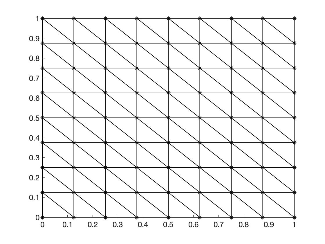
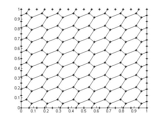
Figure 5.1: Samples of triangular (a), distorted quadrilateral (b), and hexagonal (c) meshes employed for the numerical tests in this section.

5.1 Verification of spatial convergence

First we consider a steady version of the poroelasticity equations. An exact solution of the problem on the square domain $(0,1)^{2}$ is given by the smooth functions

$$\boldsymbol{u}(x,y)=\begin{pmatrix}-\cos(2\pi x)\;\sin(2\pi y)+\sin(2\pi y)+\sin^{2}(\pi x)\sin^{2}(\pi y)\\ \sin(2\pi x)\cos(2\pi y)-\sin(2\pi x)\end{pmatrix},$$

$$p(x,y)=\sin^{2}(\pi x)\sin^{2}(\pi y),\quad\psi(x,y)=\alpha p-\lambda\mathop{\mathrm{div}}\nolimits\boldsymbol{u}.$$

The body load $\boldsymbol{f}$ and the fluid source $\ell$ are computed by evaluating these closed-form solutions and the problem is completely characterised after specifying the model constants

$$\nu=0.3,\quad E_{c}=100,\quad\kappa=1,\quad\alpha=1,\quad c_{0}=1,$$

$$\eta=0.1,\quad\lambda=\frac{E_{c}\nu}{(1+\nu)(1-2\nu)},\quad\mu=\frac{E_{c}}{(2+2\nu)}.$$

On a sequence of successively refined grids (we have employed for this particular case, uniform triangular meshes as depicted in Figure 5.1(a)) we compute errors and convergence rates according to the meshsize and tabulating also the number of degrees of freedom (Ndof). The experimental error decay (with respect to mesh refinement) is measured using individual relative norms defined as follows:

$$e_{1}(\boldsymbol{u}):=\frac{\bigl{(}\sum_{K\in\mathcal{T}_{h}}|\boldsymbol{u}-\boldsymbol{\Pi}^{\boldsymbol{\varepsilon}}_{K}\boldsymbol{u}_{h}|_{1,K}^{2}\bigr{)}^{1/2}}{|\boldsymbol{u}|_{1,\Omega}},\quad e_{0}(\boldsymbol{u}):=\frac{\bigl{(}\sum_{K\in\mathcal{T}_{h}}\|\boldsymbol{u}-\boldsymbol{\Pi}^{\boldsymbol{\varepsilon}}_{K}\boldsymbol{u}_{h}\|_{0,K}^{2}\bigr{)}^{1/2}}{\|\boldsymbol{u}\|_{0,\Omega}},$$

$$e_{1}(p):=\frac{\bigl{(}\sum_{K\in\mathcal{T}_{h}}|p-\Pi^{\nabla}_{K}p_{h}|_{1,K}^{2}\bigr{)}^{1/2}}{|p|_{1,\Omega}},\quad e_{0}(p):=\frac{\bigl{(}\sum_{K\in\mathcal{T}_{h}}\|p-\Pi^{\nabla}_{K}p_{h}\|_{0,K}^{2}\bigr{)}^{1/2}}{\|p\|_{0,\Omega}},$$

$$e_{0}(\psi):=\frac{\bigl{(}\sum_{K\in\mathcal{T}_{h}}\|\psi-\psi_{h}\|_{0,K}^{2}\bigr{)}^{1/2}}{\|\psi\|_{0,\Omega}}.$$

Table 5.1 shows this convergence history, exhibiting optimal error decay.

Ndof	$h$	$e_{1}(\boldsymbol{u})$	$r$	$e_{0}(\boldsymbol{u})$	$r$	$e_{0}(\psi)$	$r$	$e_{1}(p)$	$r$	$e_{0}(p)$	$r$
179	0.25	0.477968	-	0.271687	-	0.508386	-	0.444463	-	0.142539	-
819	0.125	0.204990	1.22	0.055766	2.28	0.198845	1.35	0.195632	1.18	0.029745	2.26
3419	0.0625	0.097838	1.07	0.013083	2.09	0.091837	1.11	0.097854	1.00	0.007526	1.98
13819	0.03125	0.049954	0.97	0.003322	1.98	0.043829	1.07	0.024456	1.02	0.001842	2.03
56067	0.015625	0.024756	1.01	$8.2\cdot 10^{-4}$	2.02	0.021704	1.01	0.024456	0.98	$4.7\cdot 10^{-4}$	1.96

Table 5.1: Verification of space convergence for the method with $k=1$. Errors and convergence rates $r$ for solid displacement, total pressure and fluid pressure.

5.2 Convergence with respect to the time advancing scheme

Regarding the convergence of the time discretisation, we fix a relatively fine hexagonal mesh and construct successively refined partitions of the time interval $(0,1]$. As in Ref. [44], and in order to avoid mixing errors coming from the spatial discretisation, we modify the exact solutions to be

$$\boldsymbol{u}(x,y,t)=100\sin(t)\begin{pmatrix}\frac{x}{\lambda}+{y},\\ x+\frac{y}{\lambda}\end{pmatrix},$$

$$p(x,y,t)=\sin(t)(x+y),\quad\psi(x,y,t)=\alpha p-\lambda\mathop{\mathrm{div}}\nolimits\boldsymbol{u},$$

and we use them to compute loads, sources, initial data, boundary values, and boundary fluxes. The model parameters assume the values

$$\kappa=0.1,\quad\alpha=1,\quad c_{0}=0,\quad\eta=1,\quad\lambda=1\times 10^{3}\quad\mu=1.$$ (5.1)

The boundary definition is $\Gamma=[\{0\}\times(0,1)]\cup[(0,1)\times\{0\}]$ (bottom and left edges) and $\Sigma=\partial\Omega\setminus\Gamma$.

We recall that cumulative errors up to $t_{\text{final}}$ associated with solid displacement, fluid pressure, and a generic pressure $v$ (representing either fluid or total pressure), are defined as

$$\begin{split}E_{0}(\boldsymbol{u})&=\biggl{(}\Delta t\sum_{n=1}^{N}\biggl{(}\sum_{K\in\mathcal{T}_{h}}\|\boldsymbol{u}(t_{n})-\boldsymbol{\Pi}^{\boldsymbol{\varepsilon}}_{K}\boldsymbol{u}^{n}_{h}\|_{0,K}^{2}\biggr{)}\biggr{)}^{1/2},\\ {E_{0}}(v)&=\biggl{(}\Delta t\sum_{n=1}^{N}\biggl{(}\sum_{K\in\mathcal{T}_{h}}\|v(t_{n})-\Pi^{\nabla}_{K}v^{n}_{h}\|_{0,K}^{2}\biggr{)}\biggr{)}^{1/2},\end{split}$$ (5.2)

respectively.

From Table 5.2 we can readily observe that these errors decay with a rate of $O(\Delta t)$.

$\Delta t$	${E_{0}}(\boldsymbol{u})$	$r$	${E_{0}}(p)$	$r$	${E_{0}}(\psi)$	$r$
0.5	0.002897	–	0.462768	–	0.398059	–
0.25	0.001362	1.09	0.218179	1.08	0.187834	1.08
0.125	$6.5173\cdot 10^{-4}$	1.06	0.104546	1.06	0.090044	1.06
0.0625	$3.1756\cdot 10^{-4}$	1.04	0.050955	1.04	0.043910	1.04
0.03125	$1.5664\cdot 10^{-4}$	1.02	0.025123	1.02	0.021683	1.02
0.015625	$7.7950\cdot 10^{-5}$	1.01	0.012469	1.01	0.010826	1.00

Table 5.2: Convergence of the time discretisation for solid displacement, fluid pressure, and total pressure, using successive partitions of the time interval and a fixed hexagonal mesh.

5.3 Verification of simultaneous space-time convergence for poroelasticity

Now we consider exact solid displacement and fluid pressure solving problem (2.1) on the square domain $\Omega=(0,1)^{2}$ and on the time interval $(0,1]$, given as

$$\boldsymbol{u}(x,y,t)=\begin{pmatrix}-\exp(-t)\sin(2\pi y)(1-\cos(2\pi x))+\frac{\exp(-t)}{\mu+\lambda}\sin(\pi x)\sin(\pi y)\\ \exp(-t)\sin(2\pi x)(1-\cos(2\pi y))+\frac{\exp(-t)}{\mu+\lambda}\sin(\pi x)\sin(\pi y)\end{pmatrix},$$

$$p(x,y,t)=\exp(-t)\sin(\pi x)\sin(\pi y),\quad\psi(x,y,t)=\alpha p-\lambda\mathop{\mathrm{div}}\nolimits\boldsymbol{u},$$

which satisfies $\mathop{\mathrm{div}}\nolimits\boldsymbol{u}\to 0$ as $\lambda\to\infty$ (see similar tests in Ref. [21, 45]). The load functions, boundary values, and initial data can be obtained from these closed-form solutions, and alternatively to the dilation modulus and permeability specified in (5.1), we here choose larger values $\lambda=1\times 10^{4}$, and $\kappa=1$.

In addition to the errors in (5.2), for displacement and for fluid pressure we will also compute

$$E_{1}(\boldsymbol{u}) =\biggl{(}\Delta t\sum_{n=1}^{N}\biggl{(}\sum_{K\in\mathcal{T}_{h}}|\boldsymbol{u}(t_{n})-\boldsymbol{\Pi}^{\boldsymbol{\varepsilon}}_{K}\boldsymbol{u}^{n}_{h}|_{1,K}^{2}\biggr{)}\biggr{)}^{1/2},$$

$$E_{1}(p) =\biggl{(}\Delta t\sum_{n=1}^{N}\biggl{(}\sum_{K\in\mathcal{T}_{h}}|p(t_{n})-\Pi^{\nabla}_{K}p^{n}_{h}|_{1,K}^{2}\biggr{)}\biggr{)}^{1/2}.$$

We consider here pure Dirichlet boundary conditions for both displacement and fluid pressure. A backward Euler time discretisation is used, and in this case we are using successive refinements of the hexagonal partition of the domain as shown in Figure 5.1(c), simultaneously with a successive refinement of the time step. The cumulative errors are again computed until the final time $t=1$, and the results are collected in Table 5.3. They show once more optimal convergence rates for the scheme in its lowest-order form.

Note from this and the previous test, that a zero constrained specific storage coefficient does not hinder the convergence properties.

$h$	$\Delta t$	$E_{1}(\boldsymbol{u})$	$r$	$E_{0}(\boldsymbol{u})$	$r$	$E_{1}(p)$	$r$	$E_{0}(p)$	$r$	$E_{0}(\psi)$	$r$
1/8	1/10	1.741116	-	0.101035	-	0.239518	-	0.009757	-	0.509493	-
1/16	1/20	0.892377	0.96	0.026166	1.95	0.123684	0.95	0.002528	1.95	0.251106	1.02
1/32	1/40	0.451402	0.98	0.006594	1.99	0.062743	0.98	0.000642	1.98	0.125025	1.01
1/64	1/80	0.227050	0.99	0.001650	2.00	0.031584	0.99	0.000161	1.99	0.062399	1.00
1/128	1/160	0.113876	1.00	0.000413	2.00	0.015844	1.00	0.000041	2.00	0.031165	1.00

Table 5.3: Convergence of the numerical method for displacement, fluid pressure, and total pressure, up to the final time $t=1$, using simultaneous partitions of the time interval and of the spatial domain (using hexagonal meshes).

5.4 Gradual compression of a poroelastic block

Finally we carry out a test involving the compression of a block occupying the region $\Omega=(0,1)^{2}$ by applying a sinusoidal-in-time traction on a small region on the top of the box (see a similar test in Ref. [38]). The model parameters in this case are

$$\nu=0.49995,\quad E_{c}=3\times 10^{4},\quad\kappa=1\times 10^{-4},\quad\alpha=1,\quad c_{0}=1\times 10^{-3},$$

$$\eta=1,\quad\lambda=\frac{E_{c}\nu}{(1+\nu)(1-2\nu)},\quad\mu=\frac{E_{c}}{(2+2\nu)}.$$

For this test we have employed a mesh conformed by distorted quadrilaterals exemplified in Figure 5.1(b). The boundary conditions are of homogeneous Dirichlet type for fluid pressure on the whole boundary, and of mixed type for displacement, and the boundary is split as $\partial\Omega:=\Gamma_{1}\cup\Gamma_{2}\cup\Gamma_{3}$. A traction $\boldsymbol{h}(t)=(0,-1.5\times 10^{4}\sin(\pi t))^{T}$ is applied on a segment of the top edge of the boundary $\Gamma_{1}=(0.25,0.75)\times\{1\}$, on the remainder of the top edge $\Gamma_{2}=[0,1]\times\{1\}\backslash\Gamma_{1}$, we impose zero traction, and the body is clamped on the remainder of the boundary $\Gamma_{3}=\partial\Omega\backslash(\Gamma_{1}\cup\Gamma_{2})$. No boundary conditions are prescribed for the total pressure. Initially the system is at rest $\boldsymbol{u}(0)=\boldsymbol{0}$, $\psi(0)=0$, $p(0)=0$, and we employ a backward Euler discretisation of the time interval $(0,0.5]$ with a constant timestep $\Delta t=0.1$. The numerical results obtained at the final time are depicted in Figure 5.2, where the profiles for fluid and total pressure present no spurious oscillations.

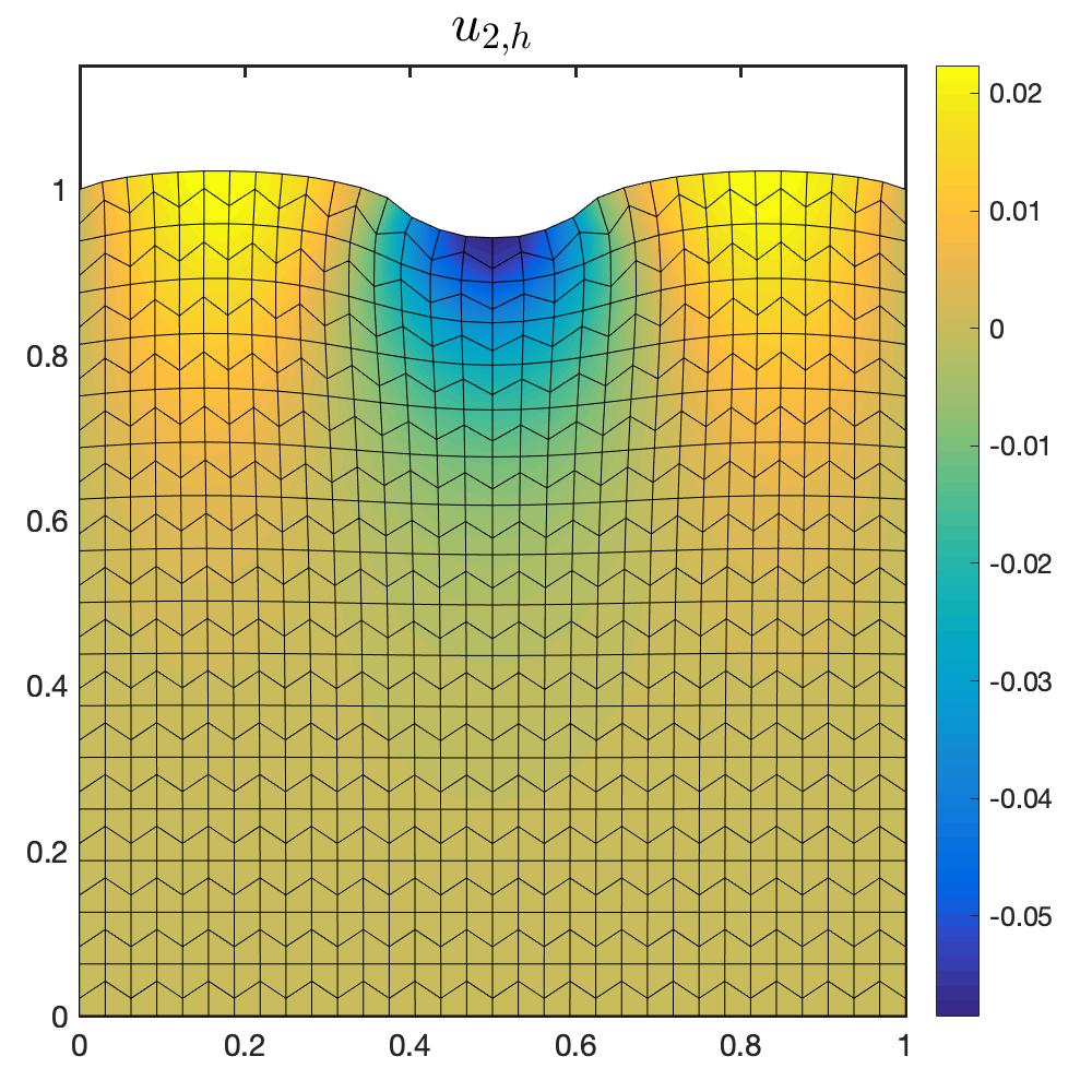
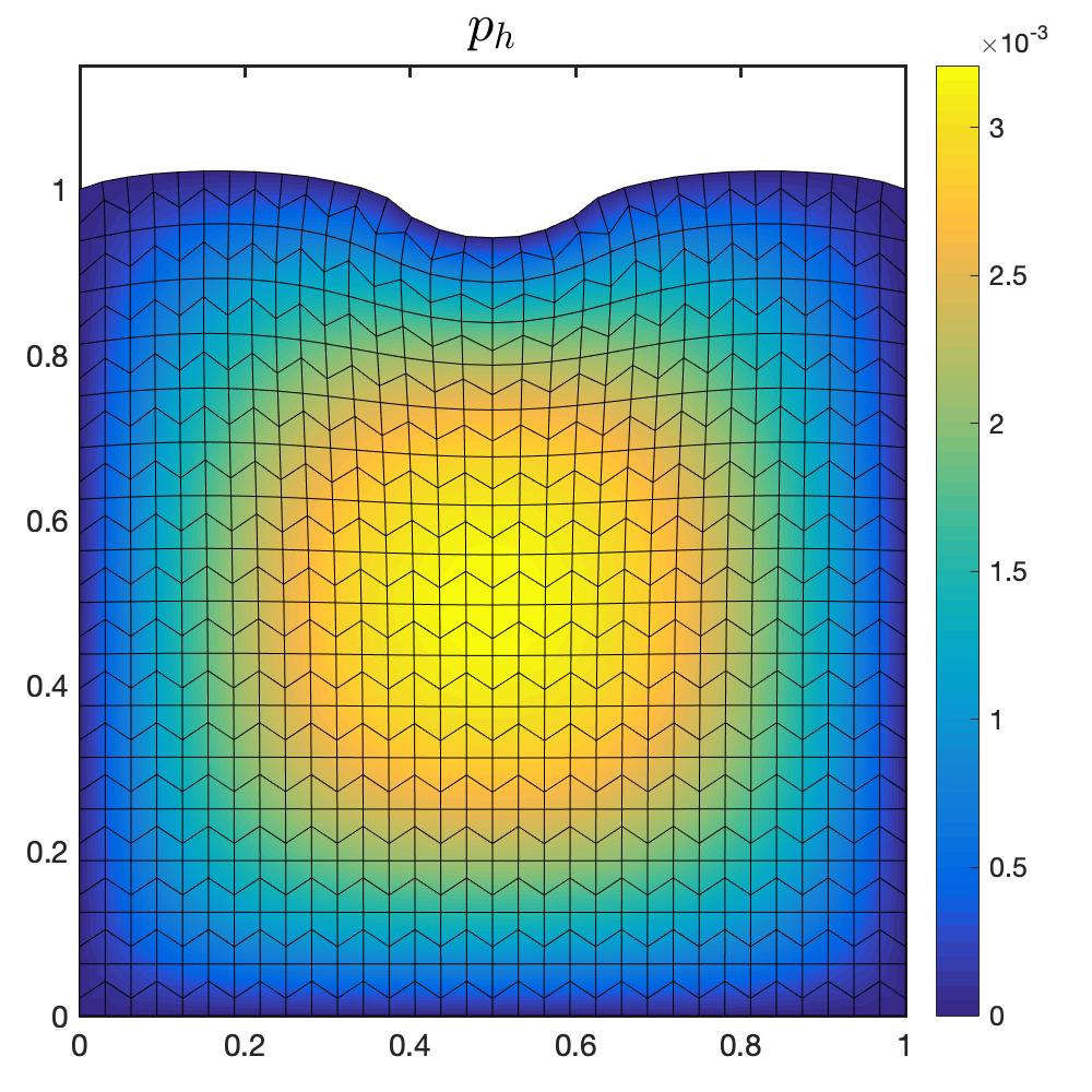
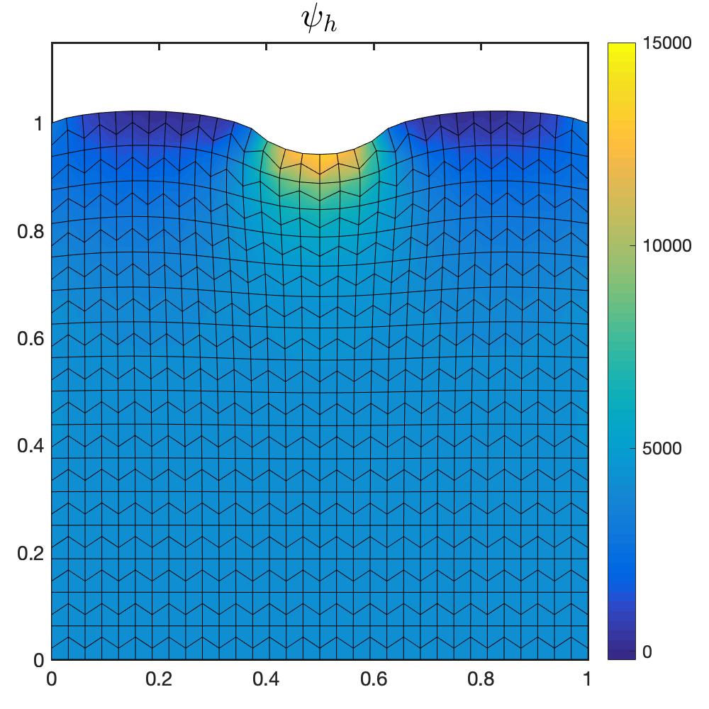
Figure 5.2: Compression of a poroelastic block after $t=0.5$ adimensional units. Approximate displacement components (a,b), displacement vectors on the undeformed domain (c), displacement magnitude (d), fluid pressure (e), and total pressure (f), depicted on the deformed domain.

6 Summary and concluding remarks

We have constructed and analysed a new virtual element method for the Biot equations of linear poroelasticity. The finite-dimensional formulation is based on Bernardi-Raugel type elements, which can be regarded as low-order and stable virtual elements, hence being computationally competitive compared to other existing stable pairs for incompressible flow problems. Both the formulation and its analysis seem to be novel, and they constitute the first fully VEM discretisation for poroelasticity problems.

Optimal and Lamé-robust error estimates were established for solid displacement, fluid pressure, and total pressure, in natural norms without weighting. This was achieved with the help of appropriate poroelastic projection operators. Numerical experiments have been performed using different polygonal meshes, and they put into evidence not only computational verification of the convergence of the scheme (where rates of error decay in space and in time are in excellent agreement with the theoretically derived error bounds), but also its performance in simple poromechanical tests.

Natural extensions of this work include the development and analysis of higher-order versions of the virtual discretisations advanced here, the efficient implementation and application to 3D problems, and the coupling with other phenomena such as diffusion of solutes in poroelastic structures[44], interface elasticity-poroelasticity problems[4], multilayer poromechanics[37], or multiple-network consolidation models[31, 26].

References

- [1] F. Aguilar, F. Gaspar, F. Lisbona, and C. Rodrigo, Numerical stabilization of Biot’s consolidation model by a perturbation on the flow equation, Int. J. Numer. Methods Engrg. 75 (2008) 1282–1300.
- [2] B. Ahmad, A. Alsaedi, F. Brezzi, L.D. Marini, and A. Russo, Equivalent projectors for virtual element methods, Comput. Math. Appl. 66 (2013) 376–391.
- [3] V. Anaya, M. Bendahmane, D. Mora, and M. Sepúlveda, A virtual element method for a nonlocal FitzHugh-Nagumo model of cardiac electrophysiology, IMA J. Numer. Anal., (2019), in press.
- [4] V. Anaya, Z. De Wijn, B. Gómez-Vargas, D. Mora, and R. Ruiz Baier, Rotation-based mixed formulations for an elasticity-poroelasticity interface problem, SIAM J. Sci. Comput., (2019), in press.
- [5] P.F. Antonietti , L. Beirão da Veiga, D. Mora, and M. Verani, A stream virtual element formulation of the Stokes problem on polygonal meshes, SIAM J. Numer. Anal. 52 (2014) 386–404.
- [6] F. Arega and E. Hayter, Coupled consolidation and contaminant transport model for simulating migration of contaminants through the sediment and a cap, Appl. Math. Model. 32 (2008) 2413–2428.
- [7] R. Asadi, B. Ataie-Ashtiani, and C.T. Simmons, Finite volume coupling strategies for the solution of a Biot consolidation model, Comput. Geotech. 55 (2014) 494–505.
- [8] L. Beirão da Veiga, F. Brezzi, A. Cangiani, G. Manzini, L.D. Marini, and A. Russo, Basic principles of virtual element methods, Math. Models Methods Appl. Sci. 23 (2013) 199–214.
- [9] L. Beirão da Veiga, F. Brezzi, and L.D. Marini, Virtual elements for linear elasticity problems, SIAM J. Numer. Anal. 51 (2013) 794–812.
- [10] L. Beirão da Veiga, F. Brezzi, L.D. Marini, and A. Russo, Virtual element method for general second-order elliptic problems on polygonal meshes, Math. Models Methods Appl. Sci. 26 (2016) 729–750.
- [11] L. Beirão da Veiga, C. Lovadina, and G. Vacca, Divergence free virtual elements for the Stokes problem on polygonal meshes, ESAIM: Math. Model. Numer. Anal. 51 (2017) 509–535.
- [12] L. Beirão da Veiga and D. Mora, A mimetic discretization of the Reissner-Mindlin plate bending problem, Numer. Math. 117 (2011) 425–462.
- [13] L. Beirão da Veiga, D. Mora, and G. Rivera, Virtual Elements for a shear-deflection formulation of Reissner-Mindlin plates, Math. Comp. 88 (2019) 149–178.
- [14] L. Berger, R. Bordas, D. Kay, and S. Tavener, Stabilized lowest-order finite element approximation for linear three-field poroelasticity, SIAM J. Sci. Comput. 37 (2015) A2222–A2245.
- [15] D. Boffi, F. Brezzi, and M. Fortin, Mixed finite element methods and applications, Springer Series in Computational Mathematics, Vol. 44, (2013) xiv+685pp.
- [16] D. Boffi, M. Botti, and D.A. Di Pietro, A nonconforming high-order method for the Biot problem on general meshes, SIAM J. Sci. Comput. 38 (2016) A1508–A1537.
- [17] S.C. Brenner and L.R. Scott, The mathematical theory of finite element methods, Texts in Applied Mathematics, Springer, New York, (2008) xviii+397pp.
- [18] A. Cangiani, E.H. Georgoulis, T. Pryer, and O.J. Sutton, A posteriori error estimates for the virtual element method, Numer. Math. 137 (2017) 857–893.
- [19] A. Cangiani, G. Manzini, and O.J. Sutton, Conforming and nonconforming virtual element methods for elliptic problems, IMA J. Numer. Anal. 37 (2017) 1317–1354.
- [20] J. Coulet, I. Faille, V. Girault, N. Guy, and F. Nataf, A fully coupled scheme using virtual element method and finite volume for poroelasticity, Comput. Geosci., (2019), in press.
- [21] G. Fu, A high-order HDG method for the Biot’s consolidation model, Comput. Math. Appl. 77 (2019) 237–252.
- [22] F.J. Gaspar, F.J. Lisbona, and P.N. Vabishchevich, Finite difference schemes for poroelastic problems, Comput. Methods Appl. Math. 2 (2002) 132–142.
- [23] V. Girault, G. Pencheva, M.F. Wheeler, and T. Wildey, Domain decomposition for poroelasticity and elasticity with DG jumps and mortars, Math. Models Methods Appl. Sci., 21 (2011) 169–213.
- [24] V. Girault and P.-A. Raviart, Finite Element Methods for Navier-Stokes Equations: Theory and algorithms. Springer Series in Computational Mathematics (1986) (5) x+374pp.
- [25] Q. Hong and J. Kraus, Parameter-robust stability of classical three-field formulation of Biot’s consolidation model, Electron. Trans. Numer. Anal. 48 (2018) 202–226.
- [26] Q. Hong, J. Kraus, M. Lymbery, and F. Philo, Conservative discretizations and parameter-robust preconditioners for Biot and multiple-network flux-based poroelasticity models. Numer. Linear Alg. Appl. 26(4) (2019) e2242.
- [27] X. Hu, C. Rodrigo, F.J. Gaspar, and L.T. Zikatanov, A non-conforming finite element method for the Biot’s consolidation model in poroelasticity, J. Comput. Appl. Math. 310 (2017) 143–154.
- [28] S. Kumar, R. Oyarzúa, R. Ruiz-Baier, and R. Sandilya, Conservative discontinuous finite volume and mixed schemes for a new four-field formulation in poroelasticity, ESAIM: Math. Model. Numer. Anal. (2019) in press.
- [29] O.A. Ladyženskaja, V.A. Solonnikov, and N.N. Ural’ ceva, Linear and Quasilinear Equations of Parabolic Type. Translated from the Russian by S. Smith. Translations of Mathematical Monographs, Vol. 23, American Mathematical Society, Providence, RI, (1968) xi+648pp.
- [30] J.J. Lee, K.-A. Mardal, and R. Winther, Parameter-robust discretization and preconditioning of Biot’s consolidation model, SIAM J. Sci. Comput. 39 (2017) A1–A24.
- [31] J.J. Lee, E. Piersanti, K.-A. Mardal, and M. Rognes, A mixed finite element method for nearly incompressible multiple-network poroelasticity, SIAM J. Sci. Comput. 41 (2019) A722–A747.
- [32] R.T. Mauck, C.T. Hung, and G.A. Ateshian, Modelling of neutral solute transport in a dynamically loaded porous permeable gel: implications for articular cartilage biosynthesis and tissue engineering, J. Biomech. Engrg. 125 (2003) 602–614.
- [33] E. Moeendarbary, L. Valon, M. Fritzsche, A.R. Harris, D.A. Moulding, A.J. Thrasher, E. Stride, L. Mahadevan, and G.T. Charras, The cytoplasm of living cells behaves as a poroelastic material, Nature Materials 12 (2013) 3517.
- [34] D. Mora and G. Rivera, A priori and a posteriori error estimates for a virtual element spectral analysis for the elasticity equations, IMA J. Numer. Anal. (2019), in press.
- [35] D. Mora, G. Rivera, and R. Rodríguez, A virtual element method for the Steklov eigenvalue problem, Math. Models Methods Appl. Sci. 25 (2015) 1421–1445.
- [36] M.A. Murad, V. Thomée, and A.F.D. Loula, Asymptotic behavior of semi discrete finite-element approximations of Biot’s consolidation problem, SIAM J. Numer. Anal. 33 (1996) 1065–1083.
- [37] A. Naumovich, On finite volume discretization of the three-dimensional Biot poroelasticity system in multilayer domains, Comput. Methods Appl. Math. 6 (2006) 306–325.
- [38] R. Oyarzúa and R. Ruiz-Baier, Locking-free finite element methods for poroelasticity, SIAM J. Numer. Anal. 54 (2016) 2951–2973.
- [39] G.P. Peters and D.W. Smith, Solute transport through a deforming porous medium, Int. J. Numer. Analytical Methods Geomech. 26 (2002) 683–717.
- [40] B. Rivière, J. Tan, and T. Thompson, Error analysis of primal discontinuous Galerkin methods for a mixed formulation of the Biot equations, Comput. Math. Appl. 73 (2017) 666–683.
- [41] R. Sacco, P. Causin, C. Lelli, and M.T. Raimondi, A poroelastic mixture model of mechanobiological processes in biomass growth: theory and application to tissue engineering, Meccanica 52 (2017) 3273–3297.
- [42] R.E. Showalter, Diffusion in poro-elastic media, J. Math. Anal. Appl. 251 (2000) 310–340.
- [43] G. Vacca and L. Beirão da Veiga, Virtual element methods for parabolic problems on polygonal meshes, Numer. Methods Partial Differential Equations 31 (2015) 2110–2134.
- [44] N. Verma, B. Gómez-Vargas, L.M. De Oliveira Vilaca, S. Kumar, and R. Ruiz-Baier, Well-posedness and discrete analysis for advection-diffusion-reaction in poroelastic media. Submitted preprint (2019). Available from arxiv.org/abs/1908.09778.
- [45] S.-Y. Yi, A study of two modes of locking in poroelasticity, SIAM J. Numer. Anal. 55 (2017) 1915–1936.