Entropy barriers and accelerated relaxation under resetting

Abstract

The zero-temperature limit of the backgammon model under resetting is studied. The model is a balls-in-boxes model whose relaxation dynamics is governed by the density of boxes containing just one particle. As these boxes become rare at large times, the model presents an entropy barrier. As a preliminary step, a related model with faster relaxation, known to be mapped to a symmetric random walk, is studied by mapping recent results on diffusion with resetting onto the balls-in-boxes problem. Diffusion with an absorbing target at the origin (and diffusion constant equal to one), stochastically reset to the unit position, is a continuum approximation to the dynamics of the balls-in-boxes model, with resetting to a configuration maximising the number of boxes containing just one ball. In the limit of a large system, the relaxation time of the balls-in-boxes model under resetting is finite. The backgammon model subject to a constant resetting rate is then studied using an adiabatic approximation.

1 Introduction

Out of-equilibrium physics has recently given rise to remarkable results on the dynamics of systems subject to resetting. The corresponding renewal equations [1, 2, 3] have a wide range of applicability and have yielded predictions in models of active matter[3, 4], predator-prey dynamics [5, 6], population dynamics [7, 8], as well as stochastic processes [9, 10, 11, 12] (see [13] for a recent review, and references therein for more applications). In particular, the expected time for a diffusive random walker in one dimension to reach an absorbing target, which is infinite in the ordinary case, is finite if the walker is stochastically reset to its initial position, at exponentially-distributed times [14].

On the other hand, glassy systems have inspired models with very slow relaxation to equilibrium. The first explicit example of these models, termed the backgammon model, involves a fixed number of distinguishable particles distributed amongst a fixed number of boxes [15, 16, 17]. At each time step (in the zero-temperature version of the model), a particle is drawn uniformly and put in another (non-empty) box. If the energy is defined as the negative of the number of empty boxes, there is no energy barrier to the relaxation of the model, as the energy can only go down. However, there is an entropy barrier: the configurations leading to a net decrease in energy (configurations in which there are boxes containing just one particle) become increasingly rare during relaxation. The occupation-number probability in non-empty boxes of this model, as well as that of a closely related model with indistinguishable particles and a faster relaxation, have been mapped to one-dimensional random walks [18], in which the position of the random walker plays the role of the occupation number. It is therefore natural to ask how results on the dynamics of random walks under resetting [1] can induce resetting prescriptions for models with entropy barriers (with computable consequences on the acceleration of the dynamics).

The paper is organised as follows. Section 2 is a review of the mapping of balls-in-boxes models without energy barrier onto random walks with an absorbing trap, introduced in [18]. This mapping applies both to the zero-temperature version of the backgammon model (termed model A), and to a related model (termed model B), in which particles are indistinguishable and the dynamics is generated by drawing departure boxes uniformly amongst non-empty boxes. Model B enjoys both faster relaxation and easier solution than model A, because it maps to a symmetric random walk (up to a density-dependent redefinition of time). In Section 3 a resetting prescription is defined, and the results of [1] on one-dimensional diffusion subject to resetting are mapped back to model B. This allows, in the limit of large systems, to calculate the relaxation time of model B under resetting. In Section 4 the resetting prescription is adapted to model A. The relaxation of model A under resetting is studied in the adiabatic approximation, using a functional expression of the generating function of the occupation-number probability. In this approximation, the relaxation dynamics of the energy is expressed in closed form in terms of the Laplace transform of the probability of occupation-number one, taken at the resetting rate. This prediction for the time evolution of the energy is compared to direct Monte Carlo simulations.

2 Description of the models

2.1 Balls-in-boxes models with entropy barriers

Consider balls-in-boxes models, in which the energy of the system is defined as the negative of the density of empty boxes (this density is the number of empty boxes divided by the total number $N$ of particles in the system). If the dynamics of a model does not allow moves that put a particle into an empty box, the energy can only decrease.

The zero-temperature version of the backgammon model [15] (called model A in [18]) is defined as follows. There are $N$ distinguishable particles distributed amongst $M$ boxes. At each time step a particle is randomly drawn (uniformly), and put into another box, randomly drawn (uniformly) from the set of the other non-empty boxes. No change of configuration involves putting a particle into an empty box; in this sense the system has no energy barrier. However, as time increases, particles tend to be taken from boxes containing large numbers of particles. Such moves do not lower the energy, hence the dynamics becomes very slow. Relaxation has an entropy barrier because moves lowering the energy (moves in which the drawn particle is alone in its box before moving) become very rare.

Consider the following related model (called model B in [18]). There are still $N$ particles distributed amongst $M$ boxes, but the particles are indistinguishable. At each time step, a departure box is randomly drawn (uniformly) from the set of non-empty boxes. A destination box is drawn uniformly among the other non-empty boxes. A particle is taken from the departure box and put into the destination box. As departure boxes are drawn uniformly, boxes containing just one particle are as likely as boxes with more particles to lose one particle. The relaxation in model B is therefore faster than in model A.

For definiteness let us consider in both models the case $N=M$. The minimum energy of the model in the limit of large systems is therefore $-1$. Let us choose the initial configuration with one particle in each box. In this configuration, every possible move decrases the energy in both models. To accelerate the dynamics by resetting the configuration of the system, we will have to pick a resetting configuration that is connected by the dynamics to the maximum possible number of states compatible with a given level of energy. This will be achieved by putting exactly one particle in each of the non-empty boxes (except one box which receives the rest of the particles). The mapping of model B to a one-dimensional diffusive random walk with an absorbing target will allow us to map the solution of the one-dimensional diffusion process under resetting to the initial position, to a solvable resetting prescription for the balls-in-boxes model.

2.2 Mapping balls-in-boxes models to random walks with an absorbing point at the origin

Let us review the derivation of [18]. An active box is defined as a non-empty box. The number of active boxes at time $\tau$ is denoted by $M(\tau)$. For any integer $k$, let us denote by $n_{k}(\tau)$ the number of active boxes at time $\tau$ containing $k$ particles. In these notations we can write:

$$\sum_{k\geq 1}n_{k}(\tau)=M(\tau),\;\;\;\;\;\;\;\sum_{k\geq 1}kn_{k}(\tau)=N.$$ (1)

As empty boxes are not active boxes, the notation implies

$$n_{0}(\tau)=0.$$ (2)

To denote the number of empty boxes, let us introduce the extra notation $n_{0}^{\ast}(\tau)$. The energy $E(\tau)$ of the system at time $\tau$ is defined as the negative of the density of empty boxes:

$$E(\tau):=-\frac{n_{0}^{\ast}(\tau)}{N}.$$ (3)

At time $\tau$, the $N$ particles are distributed amongst the $M(\tau)$ active boxes. Consider the mean density in the active boxes at time $\tau$, denoted by $\lambda(\tau)$:

$$\lambda(\tau):=\frac{N}{M(\tau)}\geq 1.$$ (4)

The lower bound is saturated if there is just one particle in each box.

Consider the density $f_{k}$ of active boxes at occupation number $k>0$, and introduce the natural notation $f_{0}^{\ast}$ for the density of empty boxes:

$$f_{k}(\tau):=\frac{n_{k}(\tau)}{N},\;\;\;\;\;\;\;f_{0}^{\ast}(\tau):=\frac{n_{0}^{\ast}(\tau)}{N},\;\;\;\;\;\;\;\;f_{0}(\tau)=0.$$ (5)

From now on let us consider the case where there are as many particles as boxes, and the initial configuration has maximal energy:

$$M=N,\;\;\;\;\;\;n_{k}(0)=\delta_{k,1}\times N.$$ (6)

These notations induce the following normalisation condition:

$$\sum_{k\geq 1}f_{k}(\tau)=\frac{M(\tau)}{N}=\frac{1}{\lambda(\tau)}=\frac{M-n_{0}^{\ast}(\tau)}{N}=1-f_{0}^{\ast}(\tau).$$ (7)

Using the definition of the energy in Eq. 3, we relate the density in active boxes $\lambda(\tau)$ to the energy of the system:

$$\frac{1}{\lambda(\tau)}=1+E(\tau).$$ (8)

3 Model B under resetting

3.1 Mapping model B to a symmetric random walk

The following master equation for the density profile of active boxes, worked out in [18], describes the dynamics of model B:

$$\begin{split}\frac{df_{k}}{d\tau}(\tau)&=\lambda(\tau)\left(f_{k+1}(\tau)-2f_{k}(\tau)+f_{k-1}(\tau)\right),\;\;\;\forall k>0.\\ f_{0}(\tau)&=0.\end{split}$$ (9)

The first term corresponds to processes that decrease the number of particles in a box with $k+1$ particles (the rate at which a box with $k+1$ particles is chosen as departure box equals $n_{k+1}(\tau)/M(\tau)=\lambda(\tau)f_{k+1}(\tau)$). The second term corresponds to processes that decrease the number of particles in a box with $k$ particles, and to processes that increase the number of particles in a box with $k$ particles. The third term corresponds to processes that increase the number of particles in a box with $k-1$ particles (the rate at which a box with $k-1$ particles is chosen as destination box equals $n_{k-1}(\tau)/M(\tau)=\lambda(\tau)f_{k-1}(\tau)$, even in the case $k=1$, because $f_{0}=0$ and empty boxes are not departure boxes).

As the mean density in the active boxes is positive, we can define a new time variable $t$ by the differential relation:

$$dt:=\lambda(\tau)d\tau,$$ (10)

which induces an expression of the original time as a function of the new time variable (see Eq. 29 for the explicit calculation of $\tau(t)$ in the system subjected to resetting). Let us reparametrise the occupation-number probability by:

$$g_{k}(t):=f_{k}\left[\tau(t)\right],\;\;\;\forall k\geq 0.$$ (11)

The time evolution described by Eq. 9 becomes a symmetric random walk with an absorbing trap at the origin:

$$\begin{split}\frac{dg_{k}}{dt}(t)&=g_{k+1}(t)-2g_{k}(t)+g_{k-1}(t),\;\;\;\;\;\forall k>0,\\ {{g_{0}(t)}}&=0.\end{split}$$ (12)

Moreover, the index $k$ (which denotes the number of particles in the active boxes) plays the role of the position of the random walker.

In the limit of an infinite number of particles, the state of the system is described by an infinite family of functions $(g_{k}(t))_{k\in\mathbf{N}}$. Let us approximate the model by a continuum, as proposed in [18], where the discrete variable $k$ become a positive variable $h$. The family of functions $(g_{k}(t))_{k\in\mathbf{N}}$ becomes a function of two variables $g(h,t)$, which satisfies the heat equation with an absorbing boundary condition at the origin:

$$\begin{split}\frac{\partial g}{\partial t}&=\frac{\partial^{2}g}{\partial h^{2}},\\ g(0,t)=0\;\;\;\;\;\forall t,&\;\;\;\;\;\;\;\;g(h^{\prime},0)=\delta(h^{\prime}-1)\;\;\;\;\;\forall h^{\prime}.\end{split}$$ (13)

The densities of boxes at integer positions are local averages of a fluctuating quantity supported on a continuum of positions, rather than on integer occupation numbers. Moreover, integrating over the position variable $h$ yields the continuous analogue of Eq. 7. The inverse of the density in active boxes (parametrised by the new time variable $t$) is therefore mapped to the survival probability of the random walker until time $t$. The propagator for the continuum random walk with an absorbing trap at the origin (conditional on the position $h^{\prime}$ at time $t=0$, and with diffusion constant equal to $1$), denoted by $p(h,t|h^{\prime},0)$, is known to be expressed as

$$p(h,t|h^{\prime},0)=\frac{1}{\sqrt{4\pi t}}\left[\exp\left(-\frac{(h-h^{\prime})^{2}}{4t}\right)-\exp\left(-\frac{(h+h^{\prime})^{2}}{4t}\right)\right].$$ (14)

The continuum approximation to the density of active boxes (as expressed in Eq. 7) is therefore obtained in integral form:

$$\frac{1}{\lambda(t)}=\int_{0}^{\infty}dhg(h,t)=\int_{0}^{\infty}dh\int_{0}^{\infty}dh^{\prime}p(h,t|h^{\prime},0)g(h^{\prime},0)=\int_{0}^{\infty}dhp(h,t|1,0).$$ (15)

3.2 Resetting prescription

Consider a resetting process of the continuous random walk, which brings the system back to the initial configuration, at random times (with a constant rate in the time variable $t$, defined by density-dependent rescaling in Eq. 10). The position of the corresponding random walker is reset to $h=1$ at each resetting event. The analogue of the position of the random walker with an absorbing target at the origin is the occupation number of boxes, and the analogue of the survival probability is the quantity $\lambda^{-1}$ (the default to the minimum energy, Eq. 8). We would like to achieve faster relaxation towards configurations of lower energy. The energy can only decrease if there are boxes containing just one particle. Moreover, the dynamics of the model implies that the energy can only decrease over time. We would therefore like to define a resetting process in the balls-and-boxes model that does not modify the energy of the system (such a modification would directly advance the relaxation process at each resetting event). From a phase-space perspective, the system is in a certain level set of given energy. The resetting prescription should put the system at the boundary of this level set. Such a prescription would lift the entropy barrier by putting the system in a state that is close to as many states of lower energy as possible.

The resetting configuration should therefore have as much of the residual probability as possible in the lowest non-zero occupation number. This is achieved by resetting the occupation numbers of all the active boxes (except one) to one. The last active box receives the rest of the particles. If the resetting occurs when the system is in a configuration with occupation numbers $(n_{0}^{\ast},n_{1},\dots,n_{N})$, with $n_{0}^{\ast}>0$, the configuration $\overrightarrow{n}^{(R)}$ of the system after resetting reads

$$\overrightarrow{n}^{(R)}=(n_{0}^{\ast},n_{1}^{(R)},0,\dots,0,n_{N-n_{1}^{(R)}}=1),\;\;\;\;\;{\mathrm{with}}\;\;\;\;\;N=n_{0}^{\ast}+n_{1}^{(R)}+1.$$ (16)

In this resetting configuration, there are therefore $n_{1}^{(R)}=N-n_{0}^{\ast}-1$ boxes with one particle, and one box with $n_{0}^{\ast}+1$ particles. The number of empty boxes in conserved by the resetting event, as required. The resetting configuration therefore depends only on the energy of the system at resetting time (up to a permutation of the boxes, but the model has no spatial structure, so for definiteness we chose the box with more than one particle to be at the end of the array of active boxes). In terms of the occupation-number probability, the resetting configuration corresponds to

$$f_{1}=1-\frac{1}{N}-\frac{n_{0}^{\ast}}{N}=\frac{1}{\lambda}-\frac{1}{N}=\frac{1}{\lambda}\left(1-\frac{\lambda}{N}\right),\;\;\;\;\;\;f_{N-n_{0}^{\ast}-1}=\frac{1}{N},$$ (17)

which sum to the residual probability of survival $1/\lambda$ at resetting time.

3.3 Renewal equation

Let us denote by $1/\lambda^{(r)}(t)$ the survival probability at time $t$ in the process with resetting (occurring at constant rate $r$ in the time variable $t$), and by $1/\lambda^{(0)}(t)$ the (known) survival probability at time $t$ in the process without resetting. In the time interval $[0,t]$, there has been either no resetting, or at least one resetting. The last of these resetting events happened at time $t-\chi$, for some time $\chi$ in $[0,t]$. These two mutually-exclusive cases give rise to the two terms on the r.h.s of the following renewal equation [1, 3]:

$$\frac{1}{\lambda^{(r)}(t)}=e^{-rt}\frac{1}{\lambda^{(0)}(t)}+r\int_{0}^{t}d\chi e^{-r\chi}Q_{0}(\chi|R)\frac{1}{\lambda^{(r)}(t-\chi)},$$ (18)

where the symbol $Q_{0}(\tau|R)$ denotes the probability of survival at time $\tau$ in the symmetric random walk (with absorbing target at the origin) without resetting, conditional on starting at the resetting configuration described by Eq. 17:

$${{Q_{0}(\chi|R)=\int_{0}^{\infty}dh\int_{0}^{\infty}dk\,p(h,\chi|g,0)\pi_{R}(k),}}$$ (19)

with

$${{\pi_{R}(k)=\left(1-\frac{\lambda^{(r)}(t-\chi)}{N}\right)\delta_{1}(k)+\frac{\lambda^{(r)}(t-\chi)}{N}\delta_{N-n_{0}^{\ast}-1}(k).}}$$ (20)

The propagator $p$ of the process without resetting, expressed in Eq. 14, gives rise to the relevant survival probabilities between resetting times:

$$Q_{0}(\chi|R)=\left(1-\frac{\lambda^{(r)}(t-\chi)}{N}\right)\int_{0}^{\infty}dhp(h,\chi|1,0)+\frac{\lambda^{(r)}(t-\chi)}{N}\int_{0}^{\infty}dhp(h,\chi|N-n_{0}^{\ast}-1,0),$$ (21)

$${{\frac{1}{\lambda^{(0)}(\chi)}=\int_{0}^{\infty}dhp(h,\chi|1,0)=\mathrm{erf}\left(\frac{1}{2\sqrt{\chi}}\right).}}$$ (22)

The renewal equation for the inverse density in active boxes therefore reads

$$\begin{split}\frac{1}{\lambda^{(r)}(t)}=&e^{-rt}\mathrm{erf}\left(\frac{1}{2\sqrt{t}}\right)\\ &\;\;+r\int_{0}^{t}d\chi e^{-r\chi}\left[\left(1-\frac{\lambda^{(r)}(t-\chi)}{N}\right)\mathrm{erf}\left(\frac{1}{2\sqrt{\chi}}\right)+\frac{\lambda^{(r)}(t-\chi)}{N}\mathrm{erf}\left(\frac{\frac{N}{\lambda^{(r)}(t-\chi)}-1}{2\sqrt{\chi}}\right)\right]\frac{1}{\lambda^{(r)}(t-\chi)}\\ =&e^{-rt}\mathrm{erf}\left(\frac{1}{2\sqrt{t}}\right)+r\int_{0}^{t}d\chi e^{-r\chi}\mathrm{erf}\left(\frac{1}{2\sqrt{\chi}}\right)\frac{1}{\lambda^{(r)}(t-\chi)}\\ &\;\;+\frac{r}{N}\int_{0}^{t}d\chi e^{-r\chi}\left[-\mathrm{erf}\left(\frac{1}{2\sqrt{\chi}}\right)+\mathrm{erf}\left(\frac{\frac{N}{\lambda^{(r)}(t-\chi)}-1}{2\sqrt{\chi}}\right)\right]d\chi.\end{split}$$ (23)

In the large-$N$ limit the last term is negligible and the following renewal equation is therefore satisfied by the inverse of the mean density in the active boxes:

$$\frac{1}{\lambda^{(r)}(t)}\simeq_{N\to\infty}e^{-rt}\mathrm{erf}\left(\frac{1}{2\sqrt{t}}\right)+r\int_{0}^{t}d\chi e^{-r\chi}\mathrm{erf}\left(\frac{1}{2\sqrt{\chi}}\right)\frac{1}{\lambda^{(r)}(t-\chi)}.$$ (24)

The above approximation is equivalent to neglecting the finite-size effects due to the presence of one box with more than one particle in the resetting configuration. The large-$N$ approximation was also made when the balls-in-boxes model was mapped to a random walk: in Eq. 12, the position index $k$ was allowed to take any positive value, even though by construction of the model its maximum value is $N$. When there is one box with $N$ particles the process ends because there are no other active boxes to move a particle to.

Let us denote by $Q_{r}(x_{0},t)$ the survival probability at time $t$ of a diffusive random walker (in dimension one), whose position at time $0$ is $x_{0}$, in the presence of an absorbing point at position $0$. The diffusion constant is equal to $1$, and the random walker undergoes resetting to its initial position $x_{0}$ at a rate $r$ (this is the notation used in Section 3.1 of the review [13]). Because of the initial condition and resetting configuration we have chosen in Eq. 13, we will be interested in $Q_{r}(1,t)$. This survival probability satisfies the following renewal equation [1, 2]:

$$Q_{r}(1,t)=e^{-rt}\mathrm{erf}\left(\frac{1}{2\sqrt{t}}\right)+r\int_{0}^{t}d\chi e^{-r\chi}\mathrm{erf}\left(\frac{1}{2\sqrt{\chi}}\right)Q_{r}(1,t-\chi).$$ (25)

Moreover, $Q_{r}(1,0)=1$ because the initial position of the random walk is fixed and distinct from the origin, and $(\lambda^{(r)}(0))^{-1}=1$ because the initial density in boxes is $1$, from Eq. 6. The quantities $(\lambda^{(r)}(t))^{-1}$ and $Q_{r}(1,t)$ are therefore identical in the large-$N$ limit. Let us use the results and notations of Section 3 of [13]. Taking the Laplace transform of both sides of Eq. 25 yields

$$\tilde{Q_{r}}(1,s)=\frac{1-\exp\left(-\sqrt{r+s}\right)}{s+r\exp\left(-\sqrt{r+s}\right)}.$$ (26)

Inverting the Laplace transform yields a parametric representation of the energy of the system in the new time $t$ which for large $t$ goes exponentially fast to the minimum. Let us follow again the notations of [13]: there exist two quantities $A>0$ and $s_{0}<0$, that depend on $r$ only, such that at large $t$

$$E(t)=-1+Q_{r}(1,t)=-1+Ae^{s_{0}t}.$$ (27)

Moreover, $s_{0}$ is the solution of

$$s_{0}+r\exp\left(-\sqrt{r+s_{0}}\right)=0,$$ (28)

which describes the pole structure in the Laplace transform.

On the other hand, the original time $\tau$ in the balls-in-boxes model can also be represented in terms of the parameter $t$, by integrating Eq. 10 w.r.t. the parameter $t$ (and using the fact that $(\lambda^{(r)}(t))^{-1}$ is the survival probability $Q_{r}(1,t)$, as we saw from Eqs 24 and 25):

$$\begin{split}\tau(t)&=\int_{0}^{t}\frac{1}{\lambda^{(r)}(u)}du\\ &=\int_{0}^{\infty}Q_{r}(1,u)du-\int_{t}^{\infty}Q_{r}(1,u)du\\ &\underset{t\to\infty}{\simeq}\tilde{Q_{r}}(1,0)+\frac{A}{s_{0}}e^{s_{0}t}\\ &=\frac{1}{r}(e^{\sqrt{r}}-1)+\frac{A}{s_{0}}e^{s_{0}t}.\end{split}$$ (29)

Moreover, the first term $\tilde{Q_{r}}(1,0)$ equals the mean time to absorption $\langle T\rangle$ (indeed this mean time is the integral of time $t$ against the negative of the time derivative of the survival probability $Q_{r}(1,t)$, which is expressed as a Laplace transform upon integration by parts). We have to eliminate the parameter $t$ from the two parametric representations found in Eqs 27 and 29:

$$1+E(t)\underset{t\to\infty}{\simeq}Ae^{s_{0}t},\;\;\;\;\;\;\;\;\tau(t)\underset{t\to\infty}{\simeq}\langle T\rangle+A\frac{e^{s_{0}t}}{s_{0}}.$$ (30)

Hence the minimum energy is approached when the real time gets close to $\tilde{Q_{r}}(1,0)$:

$$E(\tau)\simeq-1+s_{0}(\tau-\langle T\rangle),\;\;\;\;\;\;\;\;\tau\to\langle T\rangle^{-}.$$ (31)

The process relaxes therefore in finite real time if it is reset at a rate proportional to the mean density in the non-empty boxes. The constant rate of resetting in the variable $t$ implies that the typical interval of real time between resets (corresponding to an interval of $r^{-1}$ in the variable $t$) goes to zero towards the end of the relaxation (proportionally to the default to the minimum value):

$$\tau(t+r^{-1})-\tau(t)\underset{t\to\infty}{\simeq}-\frac{A}{r}e^{s_{0}t}\simeq\frac{1}{r}\left(1+E[\tau(t)]\right).$$ (32)

4 Model A under resetting

4.1 The generating function as a functional of the density in active boxes

Consider the asymmetric random walk corresponding to the zero-temperature version of the backgammon model. We know from [18] that it satisfies the following master equation:

$$\frac{df_{k}}{d\tau}(\tau)=(k+1)f_{k+1}-(\lambda(\tau)+k)f_{k}(\tau)+\lambda(\tau)f_{k-1}(\tau),\;\;\;\;\;\forall k\geq 1.$$ (33)

The first term corresponds to processes that decrease the occupation number in a box with $k+1$ particles. The total rate of these processes is the product of the occupation number in such boxes (because a particle is picked at every step), by the density of these boxes. The product $kf_{k}(\tau)$ is the contribution of processes that decrease the occupation number in a box with $k$ particles, and it comes with a minus sign because these processes decrease the density $f_{k}$. The term $\lambda(\tau)f_{k-1}(\tau)=n_{k-1}(\tau)/M(\tau)$ corresponds to processes that increase the occupation number in a box with $k-1$ particles: it is the probability that the destination box of contains $k-1$ particles. The product $\lambda(\tau)f_{k}(\tau)$ is the probability that the destination box contains $k$ particles. It corresponds to processes that increase the occupation number of a box with $k$ particles, and therefore comes with a minus sign.

Again $f_{0}(\tau)$=0, hence the model is mapped to a one-dimensional random walk with an absorbing target at the origin, but there is a density-dependent bias. The sum of the above equations over $k$ yields, using the expression given in Eq. 7 for the mean density $\lambda(\tau)$ in active boxes:

$$\frac{d}{d\tau}\left(\frac{1}{\lambda(\tau)}\right)=-f_{1}(\tau).$$ (34)

The dynamics of the model therefore slows down when the number of boxes with just one particle in them decreases.

Consider the following function, which is the sum of the generating function of the process with absorbing condition at $k=0$, and the density of inactive boxes:

$$G(y,\tau)=f_{0}^{\ast}(\tau)+\sum_{k\geq 1}f_{k}(\tau)y^{k}=1-\frac{1}{\lambda(\tau)}+\sum_{k\geq 1}f_{k}(\tau)y^{k}.$$ (35)

Summing the master equation (Eq. 33) over all possible values of $k$, and treating the order-zero term in $y$ separately, we obtain:

$$\frac{\partial G}{\partial\tau}(y,\tau)=(1-y)\left[\frac{\partial G}{\partial y}(y,\tau)-\lambda(\tau)G(y,\tau)+\lambda(\tau)-1\right].$$ (36)

Let us consider $G$ to be a functional of $\lambda$, and solve the above PDE by the method of characteristics (see [17, 15, 16, 19, 20] for an analogous approach at finite temperature). The function $\lambda$ can be adjusted by imposing the consistency condition:

$$G(0,\tau)=1-\frac{1}{\lambda(\tau)}.$$ (37)

Let us look for a change of variables from $(y,\tau)$ to $(v,\tau)$ that maps the PDE (Eq. 36) to an ODE in the time variable:

$$H(v,\tau)=G(y(v,\tau),\tau),\;\;\;\;\;\;\;\;\;\frac{\partial H}{\partial\tau}=\frac{\partial G}{\partial y}\frac{\partial y}{\partial\tau}+\frac{\partial G}{\partial\tau}.$$ (38)

Matching the combination of first derivatives in Eq. 36 yields the condition

$$\frac{\partial y}{\partial\tau}=y-1.$$ (39)

Integrating this equation, we introduce the variable $v$ as an integration constant and define the change of variables by

$$y(v,\tau)=1+ve^{\tau}.$$ (40)

The resulting ODE reads, with the function $\lambda$ treated as a parameter:

$$\frac{\partial H}{\partial\tau}=ve^{\tau}\lambda(\tau)H+ve^{\tau}(1-\lambda(\tau)).$$ (41)

Let us introduce the notation

$$\rho(\tau):=\int_{0}^{\tau}dse^{s}\lambda(s).$$ (42)

The solution of Eq. 41 reads

$$\begin{split}H(v,\tau)=&H(v,0)\exp\left(v\rho(\tau)\right)\\ &+\exp\left(v\rho(\tau)\right)\int_{0}^{\tau}dq\left[v(1-\lambda(q))e^{q}\exp\left(-v\rho(q)\right)\right].\end{split}$$ (43)

Transforming back to the variables $(y,\tau)$ yields an expression in which the first term corresponds to the initial condition (or to the last resetting configuration, as we are going to define it):

$$\begin{split}G(y,\tau)=&\;G(1+(y-1)e^{-\tau},0)\exp\left((y-1)e^{-\tau}\rho(\tau)\right)+\\ &\exp\left((y-1)e^{-\tau}\rho(\tau)\right)\int_{0}^{\tau}dq\left[(y-1)(1-\lambda(q))\exp\left(q-\tau-(y-1)e^{-\tau}\rho(q)\right)\right].\end{split}$$ (44)

4.2 Adiabatic approximation and resetting prescription

At time $\tau=0$, the boundary condition with just one particle per box reads $G(y,0)=y$, and at a resetting time $T$, we would like to accelerate the relaxation of the system to its state of minimum energy. According to Eq. 34, we can do so by maximising the number of boxes with just one particle in them (without modifying the energy of the system), just as in Eq. 17. We therefore impose, at resetting time $T$:

$$G(y,T)=1-\frac{1}{\lambda(T)}+\left(\frac{1}{\lambda(T)}{{-\frac{1}{N}}}\right)y+\frac{1}{N}y^{N(1-f_{0}^{\ast})-1}\underset{N>>1}{\simeq}1-\frac{1}{\lambda(T)}+\frac{1}{\lambda(T)}y.$$ (45)

Again, taking the large-$N$ limit amounts to neglecting the presence of just one box with more than one particle at resetting times. The density $\lambda$ is continuous at resetting times, because the resetting prescription does not change the number of empty boxes.

There are two dynamical time scales in the problem: one is the relaxation of the occupation-number probability to a quasi-stationary (density-dependent) distribution, the other one is the characteristic time of variation of the density. Let us assume that these two time scales decouple and that the time $\tau$ in Eq. 44 is small compared to the characteristic time of variation of the density $\lambda$. This is the adiabatic approximation that was proposed in the ordinary case [16]. This approximation should be even more valid in a system with resetting, because each resetting event probes short lengths of time. However, we need to take into account the short relaxation time scale towards the stationary distribution of the occupation number $k$ (which can be safely taken as Poissonian with parameter $\lambda(\tau)$ in the ordinary case [16, 18]). The adiabatic approximation on short time scales amounts to substituting the constant density

$$\Lambda:=\lambda(0)\simeq\lambda(\tau)$$ (46)

to all occurrences of the density $\lambda$ in Eq. 44. We are going to make this approximation (instead of imposing the closure condition of Eq. 37).

$$\begin{split}G(y,\tau)=G(1&+(y-1)e^{-\tau},0)\exp\left((y-1)\Lambda\int_{0}^{\tau}dse^{s-\tau}\right)+\\ &(y-1)(1-\Lambda)\int_{0}^{\tau}dq\exp\left(q-\tau+(y-1)\Lambda\int_{q}^{\tau}dse^{s-\tau}\right)\\ =G(1&+(y-1)e^{-\tau},0)\exp\left((y-1)\Lambda(1-e^{-\tau})\right)+\\ &(y-1)(1-\Lambda)\int_{0}^{\tau}dq\exp\left(q-\tau+(y-1)\Lambda(1-e^{q-\tau})\right).\end{split}$$ (47)

The last integral can be worked out explicitly:

$$\int_{0}^{\tau}dq\exp\left(q-\tau+(y-1)\Lambda(1-e^{q-\tau})\right)=\exp\left(-\tau+(y-1)\Lambda\right)\times\int_{0}^{\tau}dq\exp\left(q-(y-1)\Lambda e^{-\tau}e^{q}\right),$$ (48)

$$\int_{0}^{\tau}dqe^{q}\exp(-(y-1)\Lambda e^{-\tau}e^{q})=-\frac{e^{\tau}}{(y-1)\Lambda}\left[\exp(-(y-1)\Lambda)-\exp(-(y-1)\Lambda e^{-\tau})\right].$$ (49)

Substituting into the expression of the generating function yields:

$$\begin{split}G(y,\tau)=&\;G(1+(y-1)e^{-\tau},0)\exp\left((y-1)\Lambda(1-e^{-\tau})\right)\\ &+\left(1-\frac{1}{\Lambda}\right)\left[1-\exp((y-1)\Lambda(1-e^{-\tau}))\right].\end{split}$$ (50)

Let us assume that the last resetting event happened at time $0$, when the density in active boxes was $\lambda(0)=\Lambda$. The boundary condition is therefore given by Eq. 45, which yields:

$$\begin{split}G(y,\tau)=&\left(1-\frac{e^{-\tau}}{\Lambda}+\frac{e^{-\tau}}{\Lambda}y\right)\exp\left((y-1)\Lambda(1-e^{-\tau})\right)\\ &+\left(1-\frac{1}{\Lambda}\right)\left[1-\exp\left((y-1)\Lambda(1-e^{-\tau})\right)\right]\\ \end{split}$$ (51)

Let us introduce the shorthand notation:

$$L:=\Lambda(1-e^{-\tau}).$$ (52)

The quantity $L$ depends on $\tau$, which is not reflected in the notation, but it does not depend on $y$ and it equals zero at time $\tau=0$.

$$G(y,\tau)=\left(1-\frac{e^{-\tau}}{\Lambda}+\frac{e^{-\tau}}{\Lambda}y\right)e^{-L}\exp\left(yL\right)+\left(1-\frac{1}{\Lambda}\right)\left(1-e^{-L}\exp(yL)\right).$$ (53)

We can extract the term of order $1$ in $y$ and read off $f_{1}(\tau)$ in the adiabatic approximation:

$$\begin{split}f_{1}(\tau)=&\left(1-\frac{e^{-\tau}}{\Lambda}\right)e^{-L}L+\frac{e^{-\tau}}{\Lambda}e^{-L}-\left(1-\frac{1}{\Lambda}\right)e^{-L}L\\ =&\;e^{-L}\left[\frac{e^{-\tau}}{\Lambda}(1-L)+\frac{L}{\Lambda}\right]\\ =&\;e^{-\Lambda+\Lambda e^{-\tau}}\left[\frac{e^{-\tau}}{\Lambda}(1-\Lambda(1-e^{-\tau}))+(1-e^{-\tau})\right]\\ =&\;e^{-\Lambda+\Lambda e^{-\tau}}\left[e^{-2\tau}+e^{-\tau}\left(\frac{1}{\Lambda}-2\right)+1\right].\end{split}$$ (54)

One can check that for $\tau=0$, the above quantity reduces to $1/\Lambda$, as it should according to the resetting prescription (the term of order $1$ in $y$ in Eq. 45 is the inverse of the density in active boxes). Moreover, it goes to $e^{-\Lambda}$ when $\tau$ goes to infinity, which reflects the relaxation to a discrete Poisson distribution in the absence of resetting.

Let us apply the adiabatic approximation to the system subject to resetting (at random times distributed exponentially in time $\tau$, with rate $r$). We can take the average of the variation rate of the density (Eq. 34) against the time elapsed since the previous resetting time. The probability that this time equals $\tau$, up to $d\tau$, is $re^{-r\tau}d\tau$ if the resetting rate $r$ is constant. The relaxation rate is therefore proportional to the resetting rate and to the Laplace transform of the density of active boxes at occupation number $1$, taken at the resetting rate:

$$\begin{split}-\frac{d}{d\tau}\left(\frac{1}{\lambda(\tau)}\right)|_{\lambda=\Lambda}&=r\int_{0}^{\infty}e^{-r\tau}f_{1}(\tau)d\tau\\ &=re^{-\Lambda}\int_{0}^{\infty}d\tau e^{\Lambda e^{-\tau}}\left[e^{-(r+2)\tau}+\left(\frac{1}{\Lambda}-2\right)e^{-(r+1)\tau}+e^{-r\tau}\right]\\ &=r\mathcal{L_{\tau}}\left[f_{1}(\tau)\right](r).\end{split}$$ (55)

When the resetting rate goes to zero, the value of the above product goes to the limit of the function $f_{1}$ when $\tau$ goes to infinity, which is $e^{-\Lambda}$. This is the prediction of the adiabatic approximation in the ordinary case [16, 18].

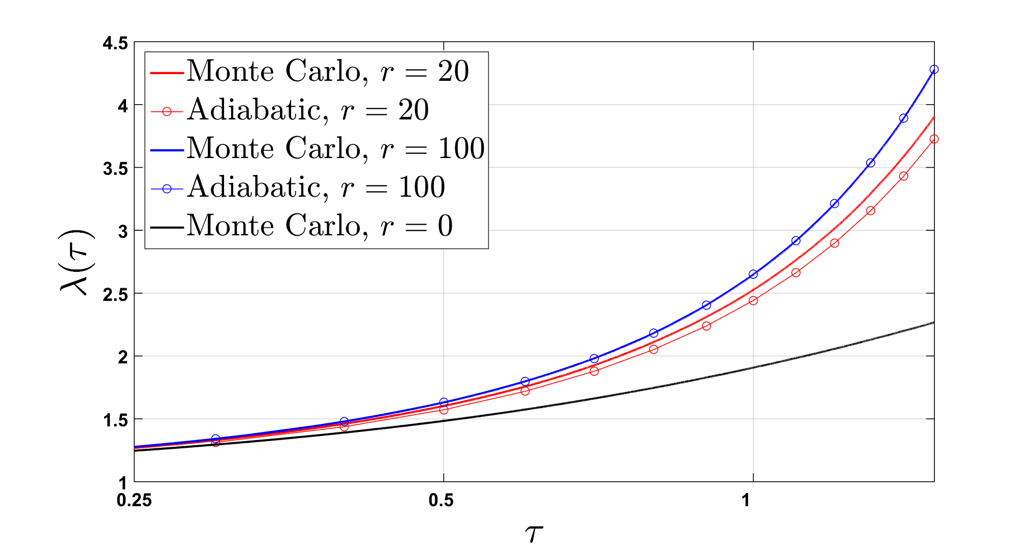
Figure 1: Density in active boxes (as a function of time $\tau$ plotted on a logarithmic scale). Number of boxes and particles $M=N=10,000$. For $r=100$ (corresponding to $1\%$ probability of resetting at each Monte Carlo time step) the predictions obtained from the adiabatic approximation are all within $0.3\%$ of the Monte Carlo result.

4.3 Numerical simulations

The dynamics of the model can be simulated directly by applying the microscopic rules to Monte Carlo samples: at each time step a particle is drawn uniformly from the system and put into a box drawn uniformly from the set of active boxes. The system is reset with a constant resetting rate in time $\tau$, to a configuration in which all active boxes except one contain just one particle. At time $\tau=0$, the density of active boxes with just one particle is $f_{1}(0)=1$. During the first Monte Carlo step, the number of active boxes decreases by one unit. The variation rate of the density induced by Eq. 34 during the first Monte Carlo step therefore reads:

$$-\frac{1}{\Delta\tau}\Delta\left(\frac{1}{\lambda(0)}\right)=-\frac{1}{\Delta\tau}\times\left(-\frac{1}{N}\right)=1.$$ (56)

The Monte Carlo time step is therefore equal to the inverse of the size of the system:

$$\Delta\tau=\frac{1}{N}.$$ (57)

On the other hand, the relaxation of the density can be predicted by integrating the adiabatic approximation numerically. Once the resetting rate $r$ has been chosen, the density is initialised at $\Lambda=1$ (according to the initial configuration chosen in Eq. 6). The r.h.s. of Eq. 55 is then evaluated (using the expression of the Laplace transform in terms of $\Lambda$ and $r$), and multiplied by the time step $\Delta\tau$. The resulting quantity is subtracted from the value of the inverse of the density. This induces a new value for the density, $\Lambda$ is updated to this new value and the process is iterated. The results of this numerical integration can be compared to the direct Monte Carlo simulation of the model (see Fig. 1 for results at $N=M=10,000$). If the resetting is strong enough, the validity of the adiabatic approximation does not crucially depend on the density $\lambda$ being large enough (which is the case is the system without resetting, because the density of boxes containing just one particle becomes exponentially small when the density becomes large). At strong resetting, taking into account the short-time relaxation dynamics of the occupation-number probabilities, as in Eq. 55, is enough to describe the relaxation of the system, as resetting probes short times, and there is only one particle moving at each Monte Carlo time step.

5 Conclusion

In this paper we have considered the effect of resetting on two models with entropy barriers. We used the known mapping of these models onto one-dimensional random walk problems with an absorbing trap at the origin, and the more recent results on diffusion with resetting. The proposed resetting prescriptions allow for a prediction of the accelerated relaxation dynamics of the original models under resetting. At each resetting event, each non-empty box receives one particle, except one which receives the rest of the particles. In the limit of a large system, this resetting configuration maps to a constant resetting position (one) of the random walker. Resetting the system lowers the entropy barrier in the same way as resetting a random walker to its initial position avoids wandering too far from the target. The entropy barrier corresponds to the fact that most of the states in a given level set of energy are far from the boundary of the level set, when the energy is low enough. At later stages of the relaxation, the system spends more and more time wandering in a fixed level set. The resetting process lifts the entropy barrier (at constant energy) by putting the system on the boundary of the current level set, at stochastic times.

In the case of the model with indistinguishable particles (termed model B in [18]), the corresponding random walk is symmetric, and upon a rescaling of time by the density in active boxes, it becomes a simple diffusion with an absorbing trap at the origin. The exact results of [1] imply that the model relaxes in finite time, with a linear approach to the minimum energy. Resetting events accumulate towards the end of the process: in an experimental procedure, the rate of resetting in real time would have to be accelerated by continuously monitoring the energy of the system (for developments on the experimental realisation of resetting prescriptions and their challenges, see [21]). On a more general note, diffusion in a phase space consisting of many metastable states (corresponding to configurations of a spin system) was shown to be logarithmic [22]. Time counted by number of moves in the system differs from real time: the typical lifetime of a state increases exponentially with the number of moves undergone by the system. For recent developments on the Glauber dynamics of spin systems in the Ising model under resetting, see [23].

In the case of the model with distinguishable particles (the zero-temperature version of the backgammon model, termed model A in [18]), the random walk is known to have position-dependent velocity and diffusion coefficient, which makes the explicit solution of the model much more difficult. An adiabatic approximation can be applied, to estimate the relaxation of the density. This approximation, introduced in [15, 18], has been adapted in this paper to the system with resetting by working out the relaxation dynamics at short time scale. On this time scale the occupation-number probability is not in a quasi-stationary state, but the density can still be treated as a constant. The time-evolution of the density has been expressed in terms of the Laplace transform (taken at the resetting rate), of the probability of occupation number one. This probability interpolates between the inverse of the density (immediately after resetting) and the inverse exponential of the density (which is the ordinary case, reached after relaxation to a Poisson distribution of the occupation numbers).

References

- [1] M. R. Evans and S. N. Majumdar, “Diffusion with stochastic resetting,” Physical review letters, vol. 106, no. 16, p. 160601, 2011.
- [2] M. R. Evans and S. N. Majumdar, “Diffusion with optimal resetting,” Journal of Physics A: Mathematical and Theoretical, vol. 44, no. 43, p. 435001, 2011.
- [3] M. R. Evans and S. N. Majumdar, “Run and tumble particle under resetting: a renewal approach,” Journal of Physics A: Mathematical and Theoretical, vol. 51, no. 47, p. 475003, 2018.
- [4] M. R. Evans and S. N. Majumdar, “Effects of refractory period on stochastic resetting,” Journal of Physics A: Mathematical and Theoretical, vol. 52, no. 1, p. 01LT01, 2018.
- [5] G. Mercado-Vásquez and D. Boyer, “Lotka–volterra systems with stochastic resetting,” Journal of Physics A: Mathematical and Theoretical, vol. 51, no. 40, p. 405601, 2018.
- [6] J. Q. Toledo-Marin, D. Boyer, and F. J. Sevilla, “Predator-prey dynamics: Chasing by stochastic resetting,” arXiv preprint arXiv:1912.02141, 2019.
- [7] P. Grange, “Steady states in a non-conserving zero-range process with extensive rates as a model for the balance of selection and mutation,” Journal of Physics A: Mathematical and Theoretical, vol. 52, no. 36, p. 365601, 2019.
- [8] P. Grange, “Non-conserving zero-range processes with extensive rates under resetting,” Journal of Physics Communications, vol. 4, no. 4, p. 045006, 2020.
- [9] G. J. Lapeyre Jr and M. Dentz, “Stochastic processes under reset,” arXiv preprint arXiv:1903.08055, 2019.
- [10] D. Gupta, “Stochastic resetting in underdamped brownian motion,” Journal of Statistical Mechanics: Theory and Experiment, vol. 2019, no. 3, p. 033212, 2019.
- [11] U. Basu, S. N. Majumdar, A. Rosso, and G. Schehr, “Long time position distribution of an active brownian particle in two dimensions,” arXiv preprint arXiv:1908.10624, 2019.
- [12] U. Basu, A. Kundu, and A. Pal, “Symmetric exclusion process under stochastic resetting,” Physical Review E, vol. 100, no. 3, p. 032136, 2019.
- [13] M. R. Evans, S. N. Majumdar, and G. Schehr, “Stochastic resetting and applications,” arXiv preprint arXiv:1910.07993, 2019.
- [14] M. R. Evans and S. N. Majumdar, “Diffusion with resetting in arbitrary spatial dimension,” Journal of Physics A: Mathematical and Theoretical, vol. 47, no. 28, p. 285001, 2014.
- [15] F. Ritort, “Glassiness in a model without energy barriers,” Physical review letters, vol. 75, no. 6, p. 1190, 1995.
- [16] S. Franz and F. Ritort, “Dynamical solution of a model without energy barriers,” EPL (Europhysics Letters), vol. 31, no. 9, p. 507, 1995.
- [17] S. Franz and F. Ritort, “Glassy mean-field dynamics of the backgammon model,” Journal of statistical physics, vol. 85, no. 1-2, pp. 131–150, 1996.
- [18] C. Godrèche, J. Bouchaud, and M. Mézard, “Entropy barriers and slow relaxation in some random walk models,” Journal of Physics A: Mathematical and General, vol. 28, no. 23, p. L603, 1995.
- [19] C. Godrèche and J. Luck, “Long-time regime and scaling of correlations in a simple model with glassy behaviour,” Journal of Physics A: Mathematical and General, vol. 29, no. 9, p. 1915, 1996.
- [20] P. Bialas, Z. Burda, and D. Johnston, “Condensation in the backgammon model,” Nuclear Physics B, vol. 493, no. 3, pp. 505–516, 1997.
- [21] O. Tal-Friedman, A. Pal, A. Sekhon, S. Reuveni, and Y. Roichman, “Experimental realization of diffusion with stochastic resetting,” arXiv preprint arXiv:2003.03096, 2020.
- [22] A. Barrat and M. Mézard, “Phase space diffusion and low temperature aging,” Journal de Physique I, vol. 5, no. 8, pp. 941–947, 1995.
- [23] M. Magoni, S. N. Majumdar, and G. Schehr, “Ising model with stochastic resetting,” arXiv preprint arXiv:2002.04867, 2020.