Role of fluctuations in the yielding transition of two-dimensional glasses

Abstract

We numerically study yielding in two-dimensional glasses which are generated with a very wide range of stabilities by swap Monte-Carlo simulations and then slowly deformed at zero temperature. We provide strong numerical evidence that stable glasses yield via a nonequilibrium discontinuous transition in the thermodynamic limit. A critical point separates this brittle yielding from the ductile one observed in less stable glasses. We find that two-dimensional glasses yield similarly to their three-dimensional counterparts but display larger sample-to-sample disorder-induced fluctuations, stronger finite-size effects, and rougher spatial wandering of the observed shear bands. These findings strongly constrain effective theories of yielding.

I Introduction

Amorphous solids encompass a wide variety of systems ranging from molecular and metallic glasses to granular media, also including foams, pastes, emulsions, and colloidal glasses. Their mechanical response to a slowly applied deformation exhibits features such as localized plastic rearrangements, avalanche-type of motion, the emergence of strain localization and shear bands Nicolas et al. (2018); Barrat and Lemaitre (2011); Rodney et al. (2011); Bonn et al. (2017); Falk and Langer (2011). The universality of these phenomena suggests that a unified description may be possible. When slowly deformed at low temperature from an initial quiescent state, amorphous solids yield beyond some finite level of applied strain and reach a steady state characterized by plastic flow. Understanding yielding is a central issue in materials science, where one would like to avoid the unwanted sudden failure of deformed glass samples Greer et al. (2013). It is also a challenging problem in nonequilibrium statistical physics Nicolas et al. (2018).

The ways in which amorphous materials yield can be classified in two main categories: the “brittle” extreme where the sample catastrophically breaks into pieces and show macroscopic shear bands Greer et al. (2013), as often observed in molecular and metallic glasses, and the “ductile” behavior in which plastic deformation increases progressively Bonn et al. (2017), commonly found in soft-matter glassy systems. The key question is whether the observed variety of yielding behaviors should be described by (i) completely distinct approaches, with, e.g., ductile yielding being describable by soft glassy rheology models Fielding et al. (2000) while brittle yielding falls into the realm of the theory of fracture Alava et al. (2006); Bouchbinder et al. (2014); Popović et al. (2018); (ii) as a unique phenomenon, taken as the ubiquitous limit of stability of a strained solid in the form of a critical spinodal Rainone et al. (2015); Urbani and Zamponi (2017); Jaiswal et al. (2016); Parisi et al. (2017), or, (iii) as we have recently argued on the basis of mean-field elasto-plastic models and simulations of a three-dimensional atomic glass Ozawa et al. (2018), within a unique theoretical framework but with the nature of yielding depending on the degree of effective disorder that is controlled by the preparation of the amorphous solid. In the latter case, and in analogy with an athermally driven random-field Ising model (RFIM) Sethna et al. (2006), yielding evolves from a mere crossover (for poorly annealed samples) to a nonequilibrium discontinuous transition past a spinodal point (for well-annealed, very stable samples); the transition between these two regimes is marked by a critical point that takes place for a specific glass preparation Nandi et al. (2016) (see also a different approach da Rocha and Truskinovsky (2020)). Here we focus on a uniform shear deformation but a similar scenario would apply to an athermal quasi-static oscillatory shear protocol Yeh et al. (2019); Bhaumik et al. (2019). Strictly speaking, these sharp transitions can only be observed at zero temperature in strain-controlled quasi-static protocols Singh et al. (2019). However, temperature is likely to play a minor role in realistic situations given the large energy scales at play. In fact, there is experimental evidence that a given material may indeed show brittle or ductile yielding depending on preparation history of the sample Shen et al. (2007); Kumar et al. (2013); Arif et al. (2012); Yang and Liu (2012); Ketkaew et al. (2018).

If yielding is a bona fide (albeit nonequilibrium) discontinuous phase transition ending in a critical point akin to that of a RFIM, one should wonder about its universality class and its dependence on space dimension. By default or with the assumption that the phenomenology is qualitatively unchanged when changing dimension, many of the numerical studies of yielding in model amorphous solids have been carried out in two dimensions (2D) Shi and Falk (2005); Maloney and Robbins (2009); Barbot et al. (2019). Whereas this may be legitimate when focusing on the flowing steady state or on very ductile behavior, one should be more cautious about the role of spatial fluctuations on the nature, and even the existence, of the yielding transition itself as one decreases the dimension of space. Fluctuations of the order parameter are expected to change the values of the exponents of the critical point as dimension is decreased below an upper critical dimension at which the mean-field description becomes qualitatively valid. More importantly, they smear the transition below a lower critical dimension. In the standard RFIM with ferromagnetic short-range interactions and short-range correlated random fields, this lower critical dimension has been proven to be $D=2$ for the equilibrium behavior Natterman (1998) and, although still debated Spasojević et al. (2011); Balog et al. (2018); Hayden et al. (2019), appears to also be $D=2$ for the out-of-equilibrium situation of the quasi-statically driven RFIM at zero temperature. However, we expect that the relevant RFIM providing an effective theory for yielding is not the standard one. It is indeed known that elastic interactions in an amorphous solids are long-ranged and anisotropic Eshelby (1957); Picard et al. (2004) instead of short-ranged ferromagnetic, as indeed shown by the appearance of strong anisotropic strain localization in the form of shear bands.

Therefore, a careful study of yielding in 2D model atomic glasses as a function of preparation is both of fundamental interest and relevant to two-dimensional physical materials, such as dry foams Arif et al. (2012), grains Ponson (2016), or silica glasses Huang et al. (2013). This is what we report in this article, where we consider glass samples that are prepared by optimized swap Monte-Carlo simulations Ninarello et al. (2017); Berthier et al. (2019) in a wide range of stability from poorly annealed glasses to very stable glasses and that are sheared through an athermal quasi-static protocol. We provide strong evidence that strained 2D stable glasses yield through a sharp discontinuous stress drop, which from finite-size scaling analysis survives in the thermodynamic limit, as in 3D. As the stability of the glass decreases, brittleness decreases and below a critical point, which is characterized by a diverging susceptibility, yielding becomes smooth. Compared to the 3D case, we find that the 2D systems are subject to larger sample-to-sample fluctuations, stronger finite-size effects, and rougher spatial wandering of the shear bands.

This paper is organized as follows. We describe the simulation methods in Sec. II. We demonstrate that two-dimensional stable glasses yield via a nonequilibrium discontinuous transition in Sec. III.1. Then we show that the brittle yielding in 2D displays larger sample-to-sample disorder-induced fluctuations with stronger finite-size effects in Sec. III.2, and rougher spatial wandering of the observed shear bands in Sec. III.3. Section III.4 presents a critical point separating the brittle and ductile yielding. Finally, we conclude our results in Sec. IV.

II Simulation methods

II.1 Model

The two-dimensional glass-forming model consists of particles with purely repulsive interactions and a continuous size polydispersity Ninarello et al. (2017); Berthier et al. (2019). Particle diameters, $d_{i}$, are randomly drawn from a distribution of the form: $f(d)=Ad^{-3}$, for $d\in[d_{\rm min},d_{\rm max}]$, where $A$ is a normalization constant. The size polydispersity is quantified by $\delta=(\overline{d^{2}}-\overline{d}^{2})^{1/2}/\overline{d}$, where the overline denotes an average over the distribution $f(d)$. Here we choose $\delta=0.23$ by imposing $d_{\rm min}/d_{\rm max}=0.449$. The average diameter, $\overline{d}$, sets the unit of length. The soft-disk interactions are pairwise and described by an inverse power-law potential

$$v_{ij}(r) = v_{0}\left(\frac{d_{ij}}{r}\right)^{12}+c_{0}+c_{1}\left(\frac{r}{d_{ij}}\right)^{2}+c_{2}\left(\frac{r}{d_{ij}}\right)^{4},$$ (1)

$$d_{ij} = \frac{(d_{i}+d_{j})}{2}(1-\epsilon|d_{i}-d_{j}|),$$ (2)

where $v_{0}$ sets the unit of energy (and of temperature with the Boltzmann constant $k_{\mathrm{B}}\equiv 1$) and $\epsilon=0.2$ quantifies the degree of nonadditivity of particle diameters. We introduce $\epsilon>0$ in the model to suppress fractionation and thus enhance the glass-forming ability. The constants $c_{0}$, $c_{1}$ and $c_{2}$ enforce a vanishing potential and continuity of its first- and second-order derivatives at the cut-off distance $r_{\rm cut}=1.25d_{ij}$. We simulate a system with $N$ particles within a square cell of area $V=L^{2}$, where $L$ is the linear box length, under periodic boundary conditions, at a number density $\rho=N/V=1$. We also compare the results with the corresponding results of the 3D system studied in Ref. [Ozawa et al., 2018].

II.2 Glass preparation

Glass samples have been prepared by first equilibrating liquid configurations at a finite temperature, $T_{\rm ini}$ (which is sometimes referred to as the fictive temperature of the glass sample) and then performing a rapid quench to $T=0$, the temperature at which the samples are subsequently deformed. We prepare equilibrium configurations for the polydisperse disks using swap Monte-Carlo simulations Berthier et al. (2016); Ninarello et al. (2017). With probability $P_{\rm swap}=0.2$, we perform a swap move where we pick two particles at random and attempt to exchange their diameters, and with probability $1-P_{\rm swap}=0.8$, we perform conventional Monte-Carlo translational moves. To perform the quench from the obtained equilibrium configurations at $T_{\rm ini}$ down to zero temperature, we use the conjugate-gradient method Nocedal and Wright (2006).

The preparation temperature $T_{\rm ini}$ then uniquely controls the stability of glass. We consider a wide range of preparation temperatures, from $T_{\rm ini}=0.035$ to $T_{\rm ini}=0.200$. To better characterize this temperature span, we give some empirically determined representative temperatures of the model: Onset of slow dynamics Sastry et al. (1998) takes place at $T_{\rm onset}\approx 0.23$, the dynamical mode-coupling crossover Götze (2008) at $T_{\rm mct}\approx 0.11$, and the estimated experimental glass transition temperature, obtained from extrapolation of the relaxation time Ninarello et al. (2017), at $T_{\rm g}\approx 0.068$. Note that these values are slightly different from the ones presented in Ref. Berthier et al. (2019) due to a small difference in the number density $\rho$. Our range of fictive temperature $T_{\rm ini}$ therefore covers from slightly below the onset temperature to significantly below the estimated experimental glass transition temperature.

II.3 Mechanical loading

We have performed strain-controlled athermal quasi-static shear (AQS) deformation using Lees-Edwards boundary conditions Maloney and Lemaître (2006). The AQS shear method consists of a succession of tiny uniform shear deformation with $\Delta\gamma=10^{-4}$, followed by energy minimization via the conjugate-gradient method. The AQS deformation is performed along the $x$-direction up to the maximum strain $\gamma_{\rm max}=0.2$. Note that during the AQS deformation, the system is always located in a potential energy minimum (except of course during the transient conjugate-gradient minimization), i.e., it stays at $T=0$.

To obtain the averaged values of the various observables, $\langle(\cdots)\rangle$, in the simulations, we average over 800, 700, 400, 200, 200, 200, 200, and 100 samples for $N=1000$, $2000$, $4000$, $8000$, $16000$, $32000$, $64000$, and $128000$, respectively. For the lowest $T_{\rm ini}=0.035$, we average over $400$ samples for $N=8000$, $16000$, $32000$, and $64000$ systems.

II.4 Nonaffine displacement

.

We consider the local nonaffine displacement of a given particle relative to its nearest neighbor particles, $D_{\rm min}^{2}$ Falk and Langer (1998). $D_{\rm min}^{2}$ is always measured between the origin ($\gamma=0$) and a given strain $\gamma$. We define nearest neighbors by using the cut-off radius of the interaction range, $R_{\rm cut}=3.0\overline{d}$. We determine the nearest neighbors of a particle from the configuration at $\gamma=0$.

III Results

III.1 Nonequilibrium discontinuous yielding transition

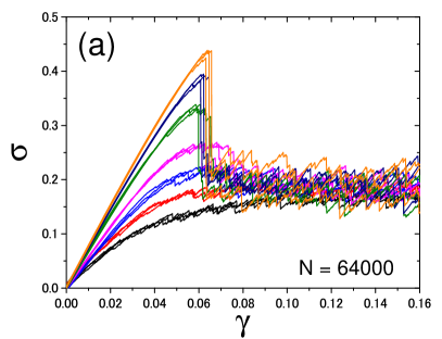
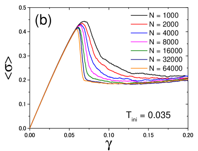
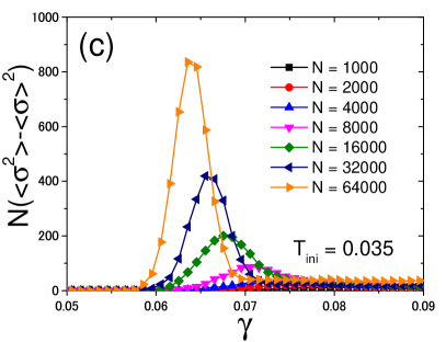
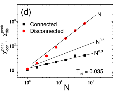
Figure 1: (a): Stress-strain curves for several typical samples of size $N=64000$ characterized for a wide span of preparation temperature $T_{\rm ini}$. From top to bottom; $T_{\rm ini}=0.035$, $0.050$, $0.070$, $0.100$, $0.120$, $0.150$, and $0.200$. For each $T_{\rm ini}$, three independent samples are shown. (b): Averaged stress-strain curves at $T_{\rm ini}=0.035$ for several values of $N$. (c): Disconnected susceptibility $\chi_{\rm dis}$ at $T_{\rm ini}=0.035$ for several values of $N$. (d): Peak values of the connected and disconnected susceptibilities, $\chi_{\rm con}^{\rm peak}$ and $\chi_{\rm dis}^{\rm peak}$, at $T_{\rm ini}=0.035$. The straight lines are the predicted scaling behaviors (see Appendix A).

Figure 1(a) shows the stress-strain curves of typical samples for several values of $T_{\rm ini}$. The curves show different types of behavior depending on the initial stability: monotonic crossover for poorly annealed samples ($T_{\rm ini}=0.150-0.200$), mild stress overshoot for ordinary computer glass samples ($T_{\rm ini}=0.100-0.120$), and a sharp discontinuous stress drop for very stable samples ($T_{\rm ini}=0.035-0.070$). This plot is qualitatively similar to that found in 3D Ozawa et al. (2018): ductile yielding is observed for higher $T_{\rm ini}$ and appears to continuously transform into brittle yielding below $T_{\rm ini}\approx 0.10-0.12$.

We first give evidence through finite-size scaling analysis that brittle yielding persists in 2D as a nonequilibrium first-order (or discontinuous) transition. For the most stable glass considered ($T_{\rm ini}=0.035$), we show in Figs. 1(b) and (c) the stress-strain curves after averaging over many samples and the so-called “disconnected” susceptibility Natterman (1998),

$$\chi_{\rm dis}=N(\langle\sigma^{2}\rangle-\langle\sigma\rangle^{2}),$$ (3)

where $\langle\cdots\rangle$ denotes an average over samples. As $N$ is increased, the slope of the drop following the stress overshoot becomes steeper, suggesting that the averaged stress-strain curve shows a discontinuous jump as $N\to\infty$. As shown below, this is due to the sudden appearance of shear bands . Concomitantly, the disconnected susceptibility $\chi_{\rm dis}$ grows with $N$. We plot its peak values as well as that of the so-called “connected” susceptibility Natterman (1998),

$$\chi_{\rm con}=-\frac{d\langle\sigma\rangle}{d\gamma}\,,$$ (4)

in Fig. 1(d). We find that both susceptibilities increase with $N$, $\chi_{\rm dis}^{\rm peak}\propto N$ and $\chi_{\rm con}^{\rm peak}\propto N^{0.3}$, which is a signature of a nonequilibrium first-order (i.e., discontinuous) transition. The stronger divergence of $\chi_{\rm dis}^{\rm peak}$ indicates the predominant role of disorder fluctuations, as generically found in the RFIM.

The observed finite-size scaling of $\chi_{\rm dis}^{\rm peak}$ is the same in 2D and 3D; it reflects the discontinuous nature of the transition where sample-to-sample stress fluctuations at a fixed yield strain are of $\mathcal{O}(1)$. On the other hand, the scaling of $\chi_{\rm con}^{\rm peak}$ is different from 3D, for which we found $\chi_{\rm con}^{\rm peak}\propto N^{0.5}$ Ozawa et al. (2018). The dominant effect explaining this difference comes from the scaling of the width of the distribution of $\gamma_{Y}$ at which the largest stress drop takes place. Sample-to-sample fluctuations seem to lead to a standard $N^{-0.5}$ behavior in 3D but to a broader distribution with a width decaying only as $N^{-0.3}$ in 2D (see Appendix A). Within a RFIM perspective Tarjus and Tissier (2008), this entails that the variance of the effective random field at the transition scales with the linear system size $L=N^{1/D}$ as

$$\Delta_{L}=\frac{\chi_{\rm dis}^{\rm peak}}{(\chi_{\rm con}^{\rm peak})^{2}}\sim L^{\rho}$$ (5)

with $\rho\approx 0.8$ in 2D and $\rho\approx 0$ in 3D. This in turn implies that the random field at yielding has long-range correlations decaying with distance as $r^{-(D-\rho)}$ with $\rho>0$ Bray (1986); Baczyk et al. (2013) in 2D, a feature that seems absent in 3D yielding. Note that the properties of the effective random field at the yielding transition result from a highly nontrivial combination of the disorder associated with the initial configurations and the evolution under deformation Rossi and Tarjus . This combination may vary with space dimension, albeit at present in a way that is not theoretically predicted.

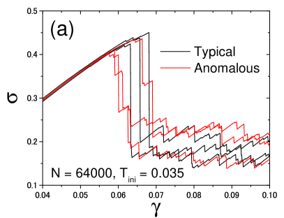
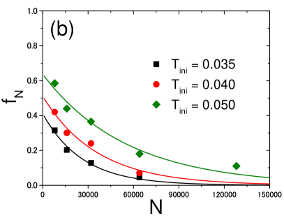
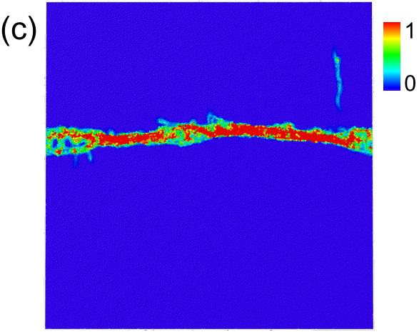
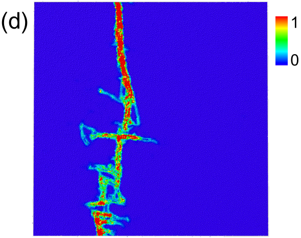
Figure 2: (a): Stress-strain curves for six samples with $N=64000$, $T_{\rm ini}=0.035$. The three black curves present typical samples showing a large stress drop. The three other red curves present rare samples showing multiple stress drops (which we call “anomalous” samples). (b): Fraction $f_{N}$ of anomalous samples as a function of $N$ for stable glasses. The solid curves are exponential fits of the data. (c, d): Representative snapshots for typical (c) and anomalous samples (d) at $\gamma=0.07$. The color bar corresponds to the value of the nonaffine displacement, $D_{\rm min}^{2}$.

III.2 Anomalous samples

To further illustrate the strong sample-to-sample fluctuations present in 2D, even in the case of very stable glasses, we show in Fig. 2(a) a zoomed-in plot of the stress-strain curves for a few chosen samples. One can see that in addition to typical samples that display a single sharp, large stress drop (see also Fig. 1(a)) there are samples that yield through multiple stress drops. These samples, which we refer to as “anomalous”, display shear bands at yielding that tend to strongly wander and splinter in space (see Fig. 2(d)), whereas typical samples yield via the appearance of a well-defined system-spanning shear band (see Fig. 2(c)) . Anomalous samples lead to very large fluctuations but their fraction, $f_{N}$, decreases as $N$ increases. To quantify this effect, we have identified these samples from individual stress-strain curves by using the conditions $\Delta\sigma_{\rm max}\leq 0.15$, where $\Delta\sigma_{\rm max}$ is the maximum stress drop observed in the strain window $\gamma\in[0,\gamma_{\rm max}]$ for each sample (see Appendix B for details). In Fig. 2(b) we observe that $f_{N}$ decreases with $N$, in an apparently exponential manner, and appears to vanish as $N\to\infty$: hence the terminology “anomalous” versus “typical”. (Note that we have checked that the finite-size scaling of $\chi_{\rm dis}^{\rm peak}$ and $\chi_{\rm con}^{\rm peak}$ in FIG. 1(d) hardly changes when we remove the anomalous samples from the computation; this shows that the observed value $\approx 0.3$ for the scaling exponent of $\chi_{\rm con}^{\rm peak}$ is not due to the presence of the anomalous samples.) Repeating the same analysis for 3D glass samples of a similar stability, we find that $f_{N}$ virtually vanishes above $N=12000$ (not shown), which indicates much weaker finite-size effects than in 2D.

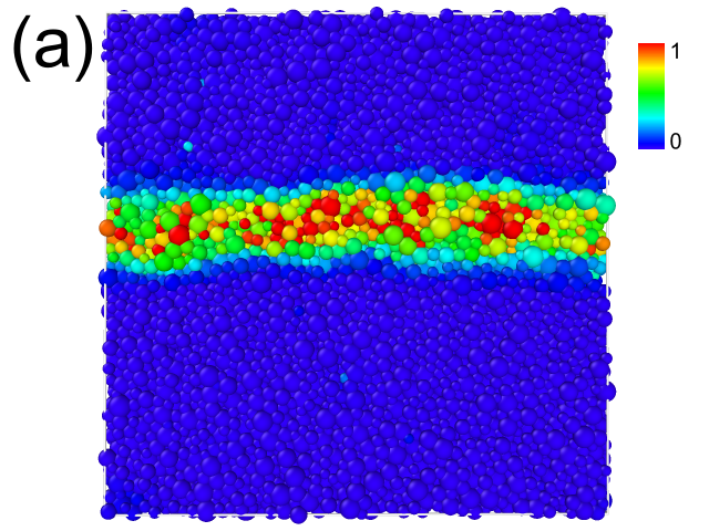
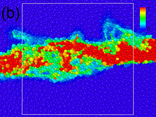
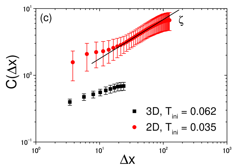
Figure 3: (a, b): Snapshot of shear bands in typical glass samples of similar stability in 3D ($N=96000$, $T_{\rm ini}=0.062$ at $\gamma=0.13$) (a) and in 2D (a zoomed-in plot of Fig. 2(c); $N=64000$, $T_{\rm ini}=0.035$ at $\gamma=0.07$) (b). The color bars correspond to the value of the nonaffine displacement $D_{\rm min}^{2}$. The white square region in (b) has the same area as the surface of the 3D simulation box. (c): Height-height correlation function $C(\Delta x)$ for 2D and 3D. The error bars correspond to the standard deviation from sample-to-sample fluctuations. The straight line corresponds to $\zeta\approx 0.59$.

III.3 Rough spacially wandering shear bands

Next, we investigate the spatial characteristics of the shear bands. We carefully analyze the wandering of the shear bands in space, comparing 2D and 3D at the same lengthscale and for similar glass stability . In Figs. 3(a) and (b), we show snapshots right after yielding for 3D ($\gamma=0.13$) and 2D ($\gamma=0.07$), respectively. The 2D shear band appears thicker than the 3D one, and a quantitative comparison is provided in the SI. More importantly, the shear band seems to wander more or, said otherwise, to be “rougher” in 2D. This roughness can be quantified by the height-height correlation function Bouchaud (1997); Ponson et al. (2006); Alava et al. (2006); Bouchbinder et al. (2006):

$$C(\Delta x)=\langle(Y_{\rm com}(x+\Delta x)-Y_{\rm com}(x))^{2}\rangle_{x}^{1/2},$$ (6)

where $Y_{\rm com}(x)$ is the average height of the shear band and $\langle\cdots\rangle_{x}$ denotes a spatial average. Note that we exclude the anomalous samples from the analysis, because defining the shear band interfaces is hard and often ambiguous in anomalous samples, e.g., when a shear band forms a closed-loop structure. For the 3D case we use an expression analogous to Eq. (6) which also takes into account the average in the additional $z$ coordinate (see Appendix D for a detailed explanation). A manifold is rough on large scales if the height-height correlation function scales with distance as $C(\Delta x)\propto\Delta x^{\zeta}$, where $\zeta>0$ is the roughness exponent. Therefore, the log-log plot of $C(\Delta x)$ versus the distance $\Delta x$ provides a way to assess the roughness of the shear bands. We show such a plot in Fig. 3(c). The data in 3D show no convincing effect over the (limited) covered range but the results in 2D point to a nontrivial intermediate regime (limited at the longest lengthscales by a saturation due to the system size) where an effective roughness exponent $\zeta\approx 0.59$ can be observed Ponson (2016). It is also clear that the overall magnitude of $C(\Delta x)$ in 2D is much larger than the one in 3D, and this difference is expected to grow even larger in larger samples. This again reflects the presence of larger spatial fluctuations in 2D.

III.4 A critical point separates brittle and ductile yielding

Because we have found strong evidence that yielding in 2D is a genuine nonequilibrium discontinuous transition for very stable glasses and that poorly annealed samples clearly show a continuous ductile behavior (see Fig. 1(a)), it is tempting to look for signatures of a critical point separating brittle and ductile yielding as one varies the preparation temperature $T_{\rm ini}$ of the glass samples. In Ref. Ozawa et al. (2018), we showed that the difference between the stress before ($\sigma_{1}$) and after ($\sigma_{2}$) the largest stress drop, $\Delta\sigma_{\rm max}=\sigma_{1}-\sigma_{2}$, plays the role of the order parameter distinguishing brittle from ductile yielding in 3D. In particular, we demonstrated that the critical point at $T_{\rm ini,c}$ can be identified by the divergence of the variance of this order parameter, $N(\langle\Delta\sigma_{\rm max}^{2}\rangle-\langle\Delta\sigma_{\rm max}\rangle^{2})$. In 2D however, as seen in Fig. 1(a), strong fluctuations seem to also affect the plastic steady state, irrespective of the presence of a critical point. Even for typical samples, this blurs the determination of the largest stress drop when the latter becomes small as one approaches the putative critical point. As an operational procedure to remove this effect, we have therefore defined the order parameter as $\Delta\sigma_{\rm max}\equiv\sigma_{1}-\langle\sigma_{2}\rangle$. In this way the fluctuations of $\sigma_{2}$ that we tentatively attribute to the plastic steady-state regime are explicitly removed. When applied to 3D this new definition captures the critical point even more sharply without affecting the results.

The mean value $\langle\Delta\sigma_{\rm max}\rangle$ is shown in Fig. 4(a) (we have removed a trivial offset at high $T_{\rm ini}$ which vanishes in the large-$N$ limit, see the inset): $\langle\Delta\sigma_{\rm max}\rangle$ appears rather flat at high $T_{\rm ini}$ and starts to grow and to develop a significant dependence on system size below $T_{\rm ini}\approx 0.1$, showing a similar trend as the 3D case. The variance of $\Delta\sigma_{\rm max}$ is displayed in Fig. 4(b). It shows a peak that grows and shifts toward higher $T_{\rm ini}$ with $N$. The data is not sufficient to allow for a proper determination of critical exponents but give nonetheless support to the existence of a brittle-to-ductile critical point around $T_{\rm ini,c}\approx 0.1$.

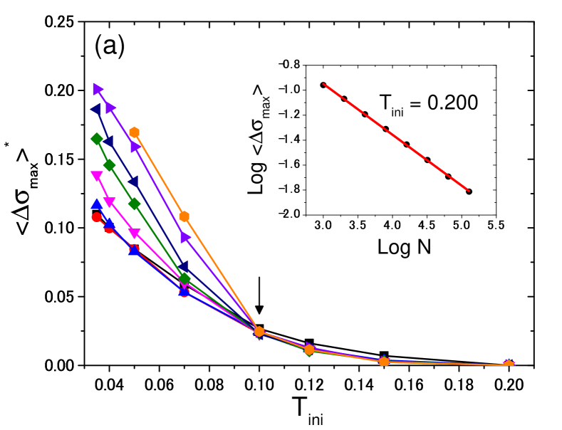
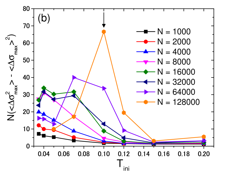
Figure 4: Mean (a) and variance (b) of the largest stress drop $\Delta\sigma_{\rm max}$ as a function of the glass preparation temperature $T_{\rm ini}$ for several system sizes $N$. In (a) we plot $\langle\Delta\sigma_{\rm max}\rangle-\langle\Delta\sigma_{\rm max}\rangle|_{T_{\rm ini}=0.2}$. We subtract the trivial high-temperature dependence that vanishes at large $N$, as shown in the inset where the data are fitted with a power law, $\langle\Delta\sigma_{\rm max}\rangle\propto N^{-0.41}$. The vertical arrows in (a) and (b) indicate the putative critical point associated with the brittle-to-ductile transition in 2D.

IV Conclusions

We have given strong numerical evidence that 2D yielding of very stable glasses under athermal quasi-static shear remains a nonequilibrium first-order (discontinuous) transition that survives in the thermodynamic limit, with a dominance of the disorder-induced, i.e., sample-to-sample, fluctuations. Furthermore, the transition to ductile yielding is signalled by a critical point. The scenario found in 2D is therefore analogous to the one found in 3D, but with stronger fluctuation effects. On the one hand, this suggests that the brittle-to-ductile transition as a function of sample preparation could be also experimentally observed in 2D or quasi-2D amorphous materials. On the other hand, it confirms that if indeed the effective theory describing the yielding transition is an athermally quasi-statically driven RFIM, the basic features of the model are necessarily modified by the presence of long-range anisotropic Eshelby-like interactions and, in 2D possibly, by long-range correlations in the effective random field. The long-range and quadrupolar nature of the elastic interactions accounts for the appearance of a shear band at the spinodal point marking the start of brittle yielding in stable glasses. In this modified RFIM, the nature of the spinodal and its potential critical character Parisi et al. (2017) still need to be investigated.

Appendix A Susceptibilities

A.1 Computation of the susceptibilities

To numerically compute the susceptibilities, we perform a smoothing procedure by averaging over 10 adjacent data points, as described in Ref. [Ozawa et al., 2018]. Figure 5 shows the parametric plot of the logarithms of the peak values of $\chi_{\rm dis}$ and $\chi_{\rm con}$. The data points roughly follow in a straight line in the putative brittle yielding phase ($T_{\rm ini}\lesssim 0.10$), with a slope of about $3$.

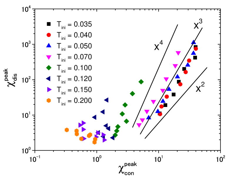
Figure 5: Parametric (log-log) plot of the peak values of the disconnected and connected susceptibilities for all system sizes and preparation temperatures. For $T_{\rm ini}\lesssim 0.10$ the logarithm of the disconnected susceptibility grows with the logarithm of the connected one.

A.2 Finite-size scaling of the susceptibilities for a discontinuous transition in the presence of disorder

We consider the case of a very stable glass (appropriate, e.g., for $T_{\rm ini}=0.035$), for which each typical finite-size sample yields through a discontinuous stress drop, $\Delta\sigma_{\rm max}$, of $\mathcal{O}(1)$ at a strain value $\gamma_{\rm Y}$. Both the size of the stress drop and the yield strain are sample dependent. It is easily realized that provided the mean value of $\langle\Delta\sigma_{\rm max}\rangle$ is strictly positive and of $\mathcal{O}(1)$, the fluctuations of $\Delta\sigma_{\rm max}$ lead only to subdominant contributions to the finite-size scaling of the susceptibilities, at least well below $T_{\rm ini,c}$. The fluctuations of the yield strain on the other hand are crucial. They are likely to regress with the system size $N$ but possibly in a nontrivial fashion. We assume that the values of $\gamma_{\rm Y}$ are distributed around the peak position, $\gamma_{\rm Y}^{*}$, of the distribution according to some probability function scaling with $N$ as

$$P_{N}(\gamma_{\rm Y})\sim N^{\delta}\mathcal{P}\left((\gamma_{\rm Y}-\gamma_{\rm Y}^{*})N^{\delta}\right),$$ (7)

with $\delta>0$ and $\mathcal{P}(0)>0$. We have computed this distribution of $\gamma_{\rm Y}$ for 2D samples prepared at $T_{\rm ini}=0.035$ and the result is shown in Fig. 6(a). We then perform exercises of scaling collapse assuming Eq. (7) with various $\delta$ in Figs. 6(b,c). We find that the conventional value, $\delta=0.5$ Procaccia et al. (2017), does not work, while a smaller value, $\delta=0.3$, provides a good scaling collapse. In the following, we will relate the obtained value, $\delta=0.3$, with the scaling of the susceptibilities.

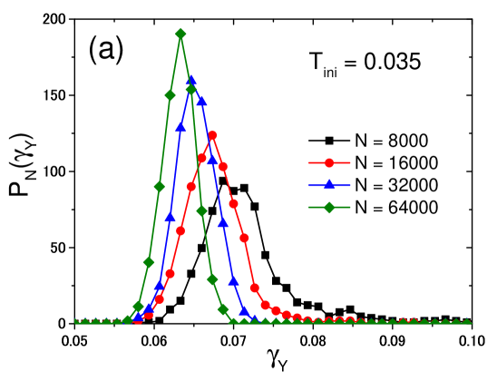
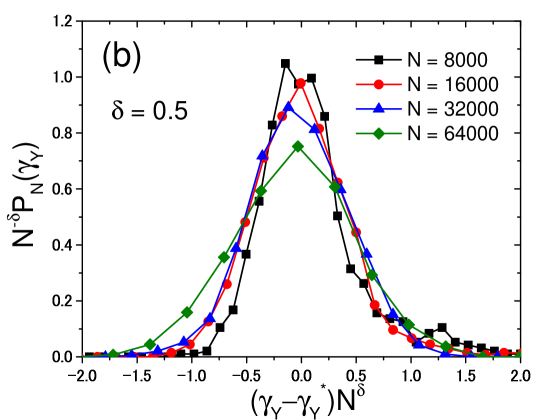
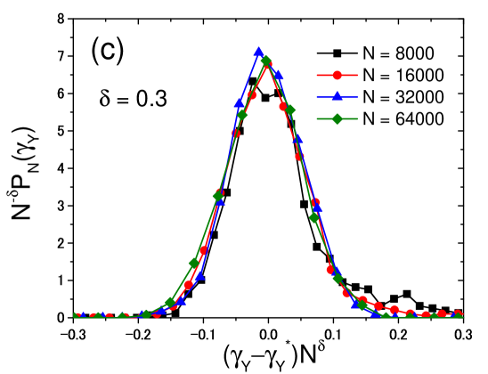
Figure 6: (a): Probability distribution of $\gamma_{\rm Y}$ determined by the position of the largest stress drop, $\Delta\sigma_{\rm max}$. (b, c): Scaling analysis assuming Eq. (7) with $\delta=0.5$ (a) and $\delta=0.3$ (b).

In the vicinity of yielding, one may describe the stress in each sample as given by

$$\sigma(\gamma)\approx\sigma_{2}+\Delta\sigma_{\rm max}\theta(\gamma_{\rm Y}-\gamma),$$ (8)

where $\theta(x)$ is the Heaviside step function and $\sigma_{2}$ is the stress right after the stress drop. As discussed in the main text, this value may also fluctuate, but just as for the fluctuations of $\Delta\sigma_{\rm max}$ this leads to only subdominant corrections to the leading finite-size scaling in the regime where a strong discontinuous transition is present. We therefore assume from now on that neither $\Delta\sigma_{\rm max}$ nor $\sigma_{2}$ fluctuate from sample to sample. One then easily derives that the first two cumulants of $\sigma(\gamma)$ close to the yielding transition are expressed as

$$\langle\sigma(\gamma)\rangle=\sigma_{2}+\Delta\sigma_{\rm max}\int_{\gamma}^{+\infty}d\gamma_{\rm Y}P_{N}(\gamma_{\rm Y}),$$ (9)

and

$$\langle\sigma(\gamma)^{2}\rangle-\langle\sigma(\gamma)\rangle^{2}=$$ (10)

$$(\Delta\sigma_{\rm max})^{2}\int_{\gamma}^{+\infty}d\gamma_{\rm Y}P_{N}(\gamma_{\rm Y})\left(1-\int_{\gamma}^{+\infty}d\gamma_{\rm Y}P_{N}(\gamma_{\rm Y})\right).$$

From the above expressions it is easy to derive the connected susceptibility,

$$\chi_{\rm con}(\gamma)=-\frac{d\langle\sigma(\gamma)\rangle}{d\gamma}=\Delta\sigma_{\rm max}P_{N}(\gamma)$$ (11)

and the disconnected one,

$$\chi_{\rm dis}(\gamma)=N\left(\langle\sigma(\gamma)^{2}\rangle-\langle\sigma(\gamma)\rangle^{2}\right)$$ (12)

$$=N(\Delta\sigma_{\rm max})^{2}\int_{\gamma}^{+\infty}d\gamma_{\rm Y}P_{N}(\gamma_{\rm Y})\left(1-\int_{\gamma}^{+\infty}d\gamma_{\rm Y}P_{N}(\gamma_{\rm Y})\right).$$

By taking now into account the scaling form of the distribution $P_{N}(\gamma_{\rm Y})$ in Eq. (7), one immediately obtains that the maximum of the susceptibilities scales as

$$\chi_{\rm con}^{\rm peak}\sim N^{\delta}\Delta\sigma_{\rm max},$$ (13)

$$\chi_{\rm dis}^{\rm peak}\sim N(\Delta\sigma_{\rm max})^{2}.$$

Putting $\delta=0.3$ obtained numerically by the scaling analysis in Fig. 6, we show a comparison between the above predictions and the directly determined $N$ dependence of $\chi_{\rm con}^{\rm peak}$ and $\chi_{\rm dis}^{\rm peak}$ in Fig. 1(d) of the main text. We find excellent agreements.

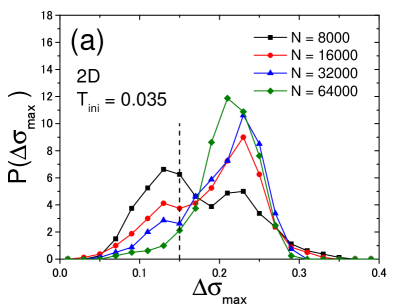
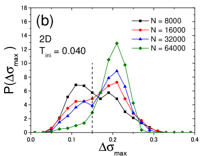
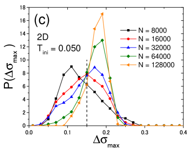
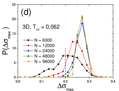
Figure 7: Probability distribution of the maximum stress drop $\Delta\sigma_{\rm max}$ at $T_{\rm ini}=0.035$ (a), $0.040$ (b), and $0.050$ (c) in 2D. The 3D model at $T_{\rm ini}=0.062$ is shown in (d) for comparison. The vertical dashed lines indicates the chosen cutoff separating typical and anomalous samples.

Appendix B Identification of the anomalous samples

Figure 7 shows the probability distribution function of the maximum stress drop $\Delta\sigma_{\rm max}$ for 2D (a,b,c) and 3D (d) for low $T_{\rm ini}$’s. For the most stable case in 2D, $T_{\rm ini}=0.035$, there are two peaks for the smaller values of $N$. The right peak correspond to samples with a single large discontinuous stress drop, which we call typical samples, and the left peak to samples with multiple stress drops at yielding, which we call anomalous samples. For $N=8000$ the peak at smaller $\Delta\sigma_{\rm max}$ is dominant, which means that the majority of samples show multiple stress drops. However, the peak at higher $\Delta\sigma_{\rm max}$ grows with increasing $N$, and for large enough system size, most of the samples show a single large discontinuous stress drop at yielding (hence the denomination of typical samples); yet there remains a tail at smaller $\Delta\sigma_{\rm max}$ corresponding to the anomalous samples. We observe the same trend up to $T_{\rm ini}=0.050$, but the peak positions shift toward smaller $\Delta\sigma_{\rm max}$ with increasing $T_{\rm ini}$. Above this $T_{\rm ini}=0.050$, we do not find any hint of two separate peaks, which forbids any sensible distinction of typical and anomalous samples.

To separate anomalous samples from typical samples for $T_{\rm ini}=0.035-0.050$, we choose a cutoff $\Delta\sigma_{\rm max}=0.15$ which seems to reasonably distinguish anomalous samples ($\Delta\sigma_{\rm max}\leq 0.15$) from typical ones ($\Delta\sigma_{\rm max}>0.15$): see Fig. 7 (a,b,c). There is some leeway in defining this cutoff value, but the conclusion in the main text does not change if we slightly change the value. In contrast to 2D, 3D systems do not show a clear bimodal distribution, as seen in Fig. 7 (d). Besides, the tail at smaller $\Delta\sigma_{\rm max}$ is significantly suppressed compared to 2D. To nonetheless make an attempt to quantify the fraction of anomalous samples, we have chosen a cutoff at $\Delta\sigma_{\rm max}=0.2$.

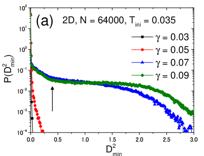
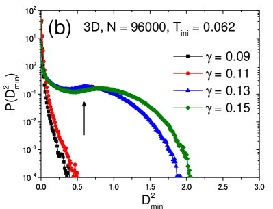
Figure 8: Probability distribution of the particle nonaffine (squared) displacement $D_{\rm min}^{2}$ in 2D (a) and in 3D (b) for several values of the strain $\gamma$ covering the regimes before and after yielding. The vertical arrows indicate the threshold above which particles are considered as belonging to a shear band: We have chosen $D_{\rm min}^{2}>0.4$ in 2D and $D_{\rm min}^{2}>0.59$ in 3D.

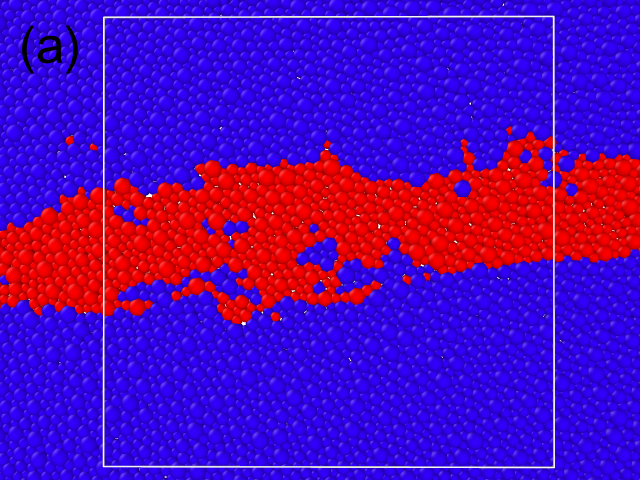
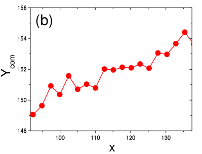
Figure 9: (a): Snapshot representing the particles belonging to a shear band (shown in red) for a 2D sample at a strain $\gamma=0.07$. The rest of the sample is essentially an elastic body and is shown in blue. (b): The $y$-coordinate of the center of mass of the shear band for each bin along the $x$-direction.

Appendix C Shear band width

We measure a typical width of the shear band, $w_{\rm SB}$, and its temperature evolution, following a similar method conducted in Refs. Parmar et al. (2019); Golkia et al. (2020). We first divide the configuration into slabs along the direction perpendicular to the shear band, and then compute the average non-affine displacement $D_{\rm min}^{2}$ for each slab. $D_{\rm min}^{2}$ is computed between the origin $\gamma=0$ and $\gamma=0.07$ ($0.13$) for 2D (3D). Figures 10(a, b) show the $D_{\rm min}^{2}$ profile obtained in 3D and 2D for several preparation temperature $T_{\rm ini}$. Clearly, the 2D systems have a wider $D_{\rm min}^{2}$ profile, in accord with the visual impression given by in Figs. 3(a,b) of the main text. Moreover, the width of the profile does not change so much along $T_{\rm ini}$ in both 3D and 2D. To quantify this feature, we operationally define $w_{\rm SB}$ as the width of the $D_{\rm min}^{2}$ profile at $D_{\rm min}^{2}=0.3$. We plot $w_{\rm SB}$ for several degrees of stability in Fig. 10(c), where $T_{\rm ini}$ is normalized by the critical preparation temperature $T_{{\rm ini},c}$ to allow a comparison between 2D and 3D cases. We find that the width $w_{\rm SB}$ in 2D is always wider than that in 3D. This conclusion does not change when considering a different normalization temperature, e.g., an estimated experimental glass transition temperature, $T_{\rm g}$.

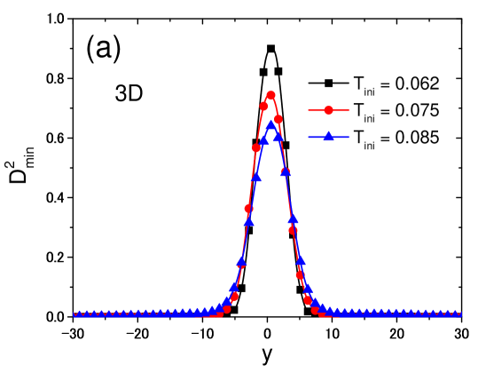
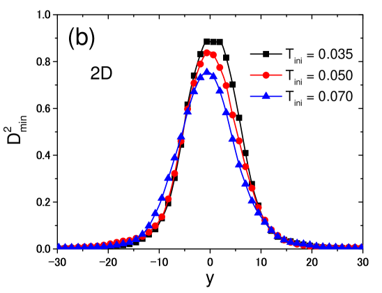
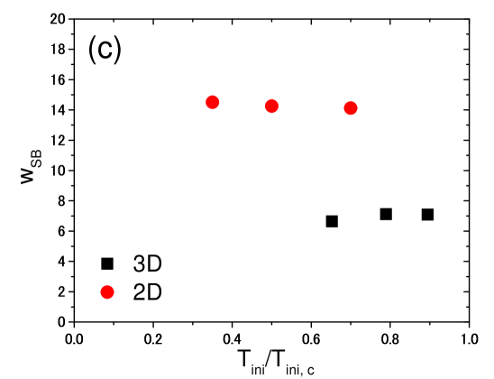
Figure 10: Averaged $D_{\rm min}^{2}$ profile along the direction perpendicular to the shear band for several preparation temperatures in 3D (a) and 2D (b). (c): Width of the shear band as a function of the normalized preparation temperature $T_{\rm ini}/T_{\rm ini,c}$.

Appendix D Roughness analysis

We present some details on how we have computed the height-height correlation function $C(\Delta x)$ for the shear bands from the molecular simulation data.

Particles are considered as part of the shear band if their nonaffine (squared) displacement $D_{\rm min}^{2}$ is large enough. Figure 8 shows the probability distribution of $D_{\rm min}^{2}$, $P(D_{\rm min}^{2})$, for several values of the strain $\gamma$ covering the regimes before and after yielding. Before yielding ($\gamma=0.03-0.05$ for 2D and $\gamma=0.09-0.11$ for 3D), $P(D_{\rm min}^{2})$ is localized near the origin, which reflects the fact that most of the particles show a purely affine deformation and that only a very small fraction of particles undergo nonaffine displacements in the pre-yield regime. After yielding ($\gamma=0.07-0.09$ for 2D and $\gamma=0.13-0.15$ for 3D) on the other hand, a significant tail suddenly appears due to strain localization in the form of shear bands, and this tail grows with increasing $\gamma$. By introducing the thresholds shown in the vertical arrows in Fig. 8, we separate particles belonging to the shear band (with a nonaffine displacement above threshold, $D_{\rm min}^{2}>0.4$ for 2D and $D_{\rm min}^{2}>0.59$ for 3D) from particles undergoing affine displacement characteristic of a purely elastic solid. An illustration is given in Fig. 9(a) for a 2D sample.

We compute the average location of the shear band (line in 2D or surface in 3D) by discretizing the base space ($x$ for a horizontal shear band in 2D, and ($x$,$z$) for a horizontal band in 3D). More specifically, we compute the $y$-coordinate of the center of mass, $Y_{\rm com}(x)$, of the particles belonging to the shear band and located within the bin specified by the position $x$ (or $x$ and $z$ in 3D). The output is illustrated in Fig. 9(b). For the bin width we have used $2.53$ in 2D and $2.28$ in 3D.

The height-height correlation functions $C(\Delta x)$ is finally defined as

$$C(\Delta x)=\langle(Y_{\rm com}(x+\Delta x)-Y_{\rm com}(x))^{2}\rangle_{x}^{1/2}$$ (14)

in 2D. In 3D where the $z$-axis has to be taken into account, the averaging procedure for $C(\Delta x)$ is also performed along the $z$-direction, according to

$$C(\Delta x)=\langle(Y_{\rm com}(x+\Delta x,z)-Y_{\rm com}(x,z))^{2}\rangle_{x,z}^{1/2}.$$ (15)

References

- Nicolas et al. (2018) Alexandre Nicolas, Ezequiel E Ferrero, Kirsten Martens, and Jean-Louis Barrat, “Deformation and flow of amorphous solids: Insights from elastoplastic models,” Reviews of Modern Physics 90, 045006 (2018).
- Barrat and Lemaitre (2011) Jean-Louis Barrat and Anael Lemaitre, “Heterogeneities in amorphous systems under shear,” Dynamical heterogeneities in glasses, colloids, and granular media 150, 264 (2011).
- Rodney et al. (2011) David Rodney, Anne Tanguy, and Damien Vandembroucq, “Modeling the mechanics of amorphous solids at different length scale and time scale,” Modelling and Simulation in Materials Science and Engineering 19, 083001 (2011).
- Bonn et al. (2017) Daniel Bonn, Morton M Denn, Ludovic Berthier, Thibaut Divoux, and Sébastien Manneville, “Yield stress materials in soft condensed matter,” Reviews of Modern Physics 89, 035005 (2017).
- Falk and Langer (2011) Michael L Falk and James S Langer, “Deformation and failure of amorphous, solidlike materials,” Annu. Rev. Condens. Matter Phys. 2, 353–373 (2011).
- Greer et al. (2013) AL Greer, YQ Cheng, and E Ma, “Shear bands in metallic glasses,” Materials Science and Engineering: R: Reports 74, 71–132 (2013).
- Fielding et al. (2000) Suzanne M Fielding, Peter Sollich, and Michael E Cates, “Aging and rheology in soft materials,” Journal of Rheology 44, 323–369 (2000).
- Alava et al. (2006) Mikko J Alava, Phani KVV Nukala, and Stefano Zapperi, “Statistical models of fracture,” Advances in Physics 55, 349–476 (2006).
- Bouchbinder et al. (2014) Eran Bouchbinder, Tamar Goldman, and Jay Fineberg, “The dynamics of rapid fracture: instabilities, nonlinearities and length scales,” Reports on Progress in Physics 77, 046501 (2014).
- Popović et al. (2018) Marko Popović, Tom WJ de Geus, and Matthieu Wyart, “Elastoplastic description of sudden failure in athermal amorphous materials during quasistatic loading,” Physical Review E 98, 040901 (2018).
- Rainone et al. (2015) Corrado Rainone, Pierfrancesco Urbani, Hajime Yoshino, and Francesco Zamponi, “Following the evolution of hard sphere glasses in infinite dimensions under external perturbations: Compression and shear strain,” Physical review letters 114, 015701 (2015).
- Urbani and Zamponi (2017) Pierfrancesco Urbani and Francesco Zamponi, “Shear yielding and shear jamming of dense hard sphere glasses,” Physical review letters 118, 038001 (2017).
- Jaiswal et al. (2016) Prabhat K Jaiswal, Itamar Procaccia, Corrado Rainone, and Murari Singh, “Mechanical yield in amorphous solids: A first-order phase transition,” Physical review letters 116, 085501 (2016).
- Parisi et al. (2017) Giorgio Parisi, Itamar Procaccia, Corrado Rainone, and Murari Singh, “Shear bands as manifestation of a criticality in yielding amorphous solids,” Proceedings of the National Academy of Sciences 114, 5577–5582 (2017).
- Ozawa et al. (2018) Misaki Ozawa, Ludovic Berthier, Giulio Biroli, Alberto Rosso, and Gilles Tarjus, “Random critical point separates brittle and ductile yielding transitions in amorphous materials,” Proceedings of the National Academy of Sciences 115, 6656–6661 (2018).
- Sethna et al. (2006) James P Sethna, Karin A Dahmen, and Olga Perkovic, “Random-field ising models of hysteresis,” in The Science of Hysteresis (Elsevier Ltd, 2006) pp. 107–179.
- Nandi et al. (2016) Saroj Kumar Nandi, Giulio Biroli, and Gilles Tarjus, “Spinodals with disorder: From avalanches in random magnets to glassy dynamics,” Physical review letters 116, 145701 (2016).
- da Rocha and Truskinovsky (2020) Hudson Borja da Rocha and Lev Truskinovsky, “Rigidity-controlled crossover: From spinodal to critical failure,” Phys. Rev. Lett. 124, 015501 (2020).
- Yeh et al. (2019) Wei-Ting Yeh, Misaki Ozawa, Kunimasa Miyazaki, Takeshi Kawasaki, and Ludovic Berthier, “Glass stability changes the nature of yielding under oscillatory shear,” arXiv preprint arXiv:1911.12951 (2019).
- Bhaumik et al. (2019) Himangsu Bhaumik, Giuseppe Foffi, and Srikanth Sastry, “The role of annealing in determining the yielding behavior of glasses under cyclic shear deformation,” arXiv preprint arXiv:1911.12957 (2019).
- Singh et al. (2019) Murari Singh, Misaki Ozawa, and Ludovic Berthier, “Brittle yielding of amorphous solids at finite shear rates,” submitted for publication (2019).
- Shen et al. (2007) J Shen, YJ Huang, and JF Sun, “Plasticity of a ticu-based bulk metallic glass: Effect of cooling rate,” Journal of Materials Research 22, 3067–3074 (2007).
- Kumar et al. (2013) Golden Kumar, Pascal Neibecker, Yan Hui Liu, and Jan Schroers, “Critical fictive temperature for plasticity in metallic glasses,” Nature communications 4, 1536 (2013).
- Arif et al. (2012) Shehla Arif, Jih-Chiang Tsai, and Sascha Hilgenfeldt, “Spontaneous brittle-to-ductile transition in aqueous foam,” Journal of Rheology 56, 485–499 (2012).
- Yang and Liu (2012) Y Yang and Chain Tsuan Liu, “Size effect on stability of shear-band propagation in bulk metallic glasses: an overview,” Journal of materials science 47, 55–67 (2012).
- Ketkaew et al. (2018) Jittisa Ketkaew, Wen Chen, Hui Wang, Amit Datye, Meng Fan, Gabriela Pereira, Udo D Schwarz, Ze Liu, Rui Yamada, Wojciech Dmowski, et al., “Mechanical glass transition revealed by the fracture toughness of metallic glasses,” Nature communications 9 (2018).
- Shi and Falk (2005) Yunfeng Shi and Michael L Falk, “Strain localization and percolation of stable structure in amorphous solids,” Physical review letters 95, 095502 (2005).
- Maloney and Robbins (2009) CE Maloney and MO Robbins, “Anisotropic power law strain correlations in sheared amorphous 2d solids,” Physical review letters 102, 225502 (2009).
- Barbot et al. (2019) Armand Barbot, Matthias Lerbinger, Anaël Lemaître, Damien Vandembroucq, and Sylvain Patinet, “Rejuvenation and shear-banding in model amorphous solids,” arXiv preprint arXiv:1906.09663 (2019).
- Natterman (1998) Thomas Natterman, “Theory of the random field ising model,” in Spin glasses and random fields (World Scientific, 1998) pp. 277–298.
- Spasojević et al. (2011) Djordje Spasojević, Sanja Janićević, and Milan Knežević, “Numerical evidence for critical behavior of the two-dimensional nonequilibrium zero-temperature random field ising model,” Phys. Rev. Lett. 106, 175701 (2011).
- Balog et al. (2018) Ivan Balog, Gilles Tarjus, and Matthieu Tissier, “Criticality of the random field ising model in and out of equilibrium: A nonperturbative functional renormalization group description,” Physical Review B 97, 094204 (2018).
- Hayden et al. (2019) LX Hayden, Archishman Raju, and James P Sethna, “Unusual scaling for two-dimensional avalanches: Curing the faceting and scaling in the lower critical dimension,” Physical Review Research 1, 033060 (2019).
- Eshelby (1957) John Douglas Eshelby, “The determination of the elastic field of an ellipsoidal inclusion, and related problems,” Proceedings of the Royal Society of London. Series A. Mathematical and Physical Sciences 241, 376–396 (1957).
- Picard et al. (2004) Guillemette Picard, Armand Ajdari, François Lequeux, and Lydéric Bocquet, “Elastic consequences of a single plastic event: A step towards the microscopic modeling of the flow of yield stress fluids,” The European Physical Journal E 15, 371–381 (2004).
- Ponson (2016) Laurent Ponson, “Statistical aspects in crack growth phenomena: how the fluctuations reveal the failure mechanisms,” International Journal of Fracture 201, 11–27 (2016).
- Huang et al. (2013) Pinshane Y Huang, Simon Kurasch, Jonathan S Alden, Ashivni Shekhawat, Alexander A Alemi, Paul L McEuen, James P Sethna, Ute Kaiser, and David A Muller, “Imaging atomic rearrangements in two-dimensional silica glass: watching silica’s dance,” science 342, 224–227 (2013).
- Ninarello et al. (2017) Andrea Ninarello, Ludovic Berthier, and Daniele Coslovich, “Models and algorithms for the next generation of glass transition studies,” Physical Review X 7, 021039 (2017).
- Berthier et al. (2019) Ludovic Berthier, Patrick Charbonneau, Andrea Ninarello, Misaki Ozawa, and Sho Yaida, “Zero-temperature glass transition in two dimensions,” Nature communications 10 (2019).
- Berthier et al. (2016) Ludovic Berthier, Daniele Coslovich, Andrea Ninarello, and Misaki Ozawa, “Equilibrium sampling of hard spheres up to the jamming density and beyond,” Phys. Rev. Lett 116, 238002 (2016).
- Nocedal and Wright (2006) Jorge Nocedal and Stephen Wright, Numerical optimization (Springer Science & Business Media, 2006).
- Sastry et al. (1998) Srikanth Sastry, Pablo G Debenedetti, and Frank H Stillinger, “Signatures of distinct dynamical regimes in the energy landscape of a glass-forming liquid,” Nature 393, 554 (1998).
- Götze (2008) Wolfgang Götze, Complex dynamics of glass-forming liquids: A mode-coupling theory, Vol. 143 (OUP Oxford, 2008).
- Maloney and Lemaître (2006) Craig E Maloney and Anaël Lemaître, “Amorphous systems in athermal, quasistatic shear,” Physical Review E 74, 016118 (2006).
- Falk and Langer (1998) Michael L Falk and James S Langer, “Dynamics of viscoplastic deformation in amorphous solids,” Physical Review E 57, 7192 (1998).
- Note (1) The () displacement along the shear band is accompanied by a change in the elastic strain energy in the bulk of the system that scales extensively with system size and explains the first-order character of the transition marked by a discontinuous stress drop of .
- Tarjus and Tissier (2008) Gilles Tarjus and Matthieu Tissier, “Nonperturbative functional renormalization group for random field models and related disordered systems. i. effective average action formalism,” Physical Review B 78, 024203 (2008).
- Bray (1986) AJ Bray, “Long-range random-field models: scaling theory and 1/n expansion,” Journal of Physics C: Solid State Physics 19, 6225 (1986).
- Baczyk et al. (2013) Maxime Baczyk, Matthieu Tissier, Gilles Tarjus, and Yoshinori Sakamoto, “Dimensional reduction and its breakdown in the three-dimensional long-range random-field ising model,” Physical Review B 88, 014204 (2013).
- (50) Saverio Rossi and Gilles Tarjus, Unpublished.
- Note (2) Note that due to the choice of periodic boundary conditions the direction of the shear band is either horizontal or vertical, with about equal probability for one or the other Kapteijns et al. (2019). We have checked that the properties of horizontal and vertical shear bands are virtually the same.
- Note (3) Similar glass stability in a sence that the ratio between the peak and steady state stress values are similar Kapteijns et al. (2019).
- Bouchaud (1997) Elisabeth Bouchaud, “Scaling properties of cracks,” Journal of Physics: Condensed Matter 9, 4319 (1997).
- Ponson et al. (2006) Laurent Ponson, Daniel Bonamy, and Elisabeth Bouchaud, “Two-dimensional scaling properties of experimental fracture surfaces,” Physical review letters 96, 035506 (2006).
- Bouchbinder et al. (2006) Eran Bouchbinder, Itamar Procaccia, Stéphane Santucci, and Loïc Vanel, “Fracture surfaces as multiscaling graphs,” Physical review letters 96, 055509 (2006).
- Procaccia et al. (2017) Itamar Procaccia, Corrado Rainone, and Murari Singh, “Mechanical failure in amorphous solids: Scale-free spinodal criticality,” Physical Review E 96, 032907 (2017).
- Parmar et al. (2019) Anshul DS Parmar, Saurabh Kumar, and Srikanth Sastry, “Strain localization above the yielding point in cyclically deformed glasses,” Physical Review X 9, 021018 (2019).
- Golkia et al. (2020) Mehrdad Golkia, Gaurav P Shrivastav, Pinaki Chaudhuri, and Jürgen Horbach, “Flow heterogeneities in supercooled liquids and glasses under shear,” arXiv preprint arXiv:2004.02868 (2020).
- Kapteijns et al. (2019) Geert Kapteijns, Wencheng Ji, Carolina Brito, Matthieu Wyart, and Edan Lerner, “Fast generation of ultrastable computer glasses by minimization of an augmented potential energy,” Physical Review E 99, 012106 (2019).