Non-perturbative renormalization by decoupling

Abstract

We propose a new strategy for the determination of the QCD coupling. It relies on a coupling computed in QCD with $N_{\mathrm{f}}\geq 3$ degenerate heavy quarks at a low energy scale $\mu_{\mathrm{dec}}$, together with a non-perturbative determination of the ratio $\Lambda/\mu_{\mathrm{dec}}$ in the pure gauge theory. We explore this idea using a finite volume renormalization scheme for the case of $N_{\rm f}=3$ QCD, demonstrating that a precise value of the strong coupling $\alpha_{s}$ can be obtained. The idea is quite general and can be applied to solve other renormalization problems, using finite or infinite volume intermediate renormalization schemes.

I Introduction

Currently the best estimates of $\alpha_{s}(m_{Z})$ reach a precision below $1\%$, with lattice QCD providing the most precise determinations Aoki et al. (2019); Maltman et al. (2008); Aoki et al. (2009); McNeile et al. (2010); Chakraborty et al. (2015); Bazavov et al. (2014); Nakayama et al. (2016); Bruno et al. (2017a). The main challenge in a solid extraction of $\alpha_{s}$ by using lattice QCD is the estimate of perturbative truncation uncertainties, other power corrections, and finite lattice spacing errors which are present in all extractions (see also Dalla Brida et al. (2016, 2018)).

A dedicated lattice QCD approach, known as step scaling Lüscher et al. (1991), allows to connect an experimentally well-measured low-energy quantity with the high energy regime of QCD where perturbation theory can be safely applied, without making any assumptions on the physics at energy scales of a few GeV. It has recently been applied to three flavor QCD, yielding $\alpha_{s}(m_{Z})$ with very high precision by means of a non-perturbative running from scales of 0.2 GeV to 70 GeV Bruno et al. (2017a); Dalla Brida et al. (2017, 2016) and perturbation theory above. Although new techniques Lüscher (2010); Fritzsch and Ramos (2013) have recently made possible a significant improvement over older computations Della Morte et al. (2005); Aoki et al. (2009); Tekin et al. (2010) a substantial further reduction of the overall error is challenging.

In this paper we propose a new strategy for the computation of the strong coupling. It is based on QCD with $N_{\mathrm{f}}\geq 3$ quarks. We take the quarks to be degenerate, with an un-physically large mass, $M$. They then decouple from the low-energy physics, which predicts our basic relation

$$\frac{\Lambda_{\rm\overline{MS\kern-0.35002pt}\kern 0.35002pt}^{(N_{\mathrm{f}})}}{\mu_{\mathrm{dec}}}\;P\left(\frac{M}{\mu_{\mathrm{dec}}}\frac{\mu_{\mathrm{dec}}}{\Lambda_{\rm\overline{MS\kern-0.35002pt}\kern 0.35002pt}^{(N_{\mathrm{f}})}}\right)=\frac{\Lambda_{\rm\overline{MS\kern-0.35002pt}\kern 0.35002pt}^{(0)}}{\Lambda_{s}^{(0)}}\,\varphi_{s}^{(0)}\left(\sqrt{u_{\mathrm{M}}}\right)+{\rm O}(M^{-2})\,,$$

(1)

as we will explain in detail. Here $u_{\mathrm{M}}=\bar{g}^{2}_{s}(\mu_{\mathrm{dec}},M)$ is the value of the coupling in a massive renormalization scheme at the scale $\mu_{\mathrm{dec}}$. The function $\varphi^{(0)}_{s}(\bar{g}(\mu_{\mathrm{dec}}))=\Lambda_{s}^{(0)}/\mu_{\mathrm{dec}}$ relates the same coupling and the renormalization scale $\mu=\mu_{\mathrm{dec}}$ in the zero-flavor theory and the function $P$ gives the ratio $\Lambda_{\rm\overline{MS\kern-0.35002pt}\kern 0.35002pt}^{(0)}/\Lambda_{\rm\overline{MS\kern-0.35002pt}\kern 0.35002pt}^{(N_{\mathrm{f}})}$. As shown in Bruno et al. (2015a); Athenodorou et al. (2019) $P$ is described very precisely by (high order) perturbation theory. The scale $\mu_{\mathrm{dec}}$ has to be small compared to $M$ but is arbitrary otherwise. To make contact to physical units of MeV for the $\Lambda$-parameter, $\mu_{\mathrm{dec}}$ has to be related to a physical mass-scale such as $\mu_{\rm phys}=m_{\mathrm{proton}}$ (at physical quark masses). The use of intermediate unphysical scales Sommer (2014) is of course possible.

In essence the above formula relates the $N_{\mathrm{f}}$-flavor $\Lambda$ parameter to the pure gauge one by means of a massive coupling. Since perturbation theory is used only at the scale $M$, it can be controlled by making $M$ sufficiently large.

The main advantage of this approach is that the non-perturbative running of $\alpha_{s}$ from $\mu_{\mathrm{dec}}$ to high energies is needed only in the pure gauge theory, where high precision can be reached, see Dalla Brida and Ramos (2019). It is connected to the three flavor theory by a perturbative approximation for $P$, which is very accurate already for masses around the charm mass, $M\approx M_{\mathrm{charm}}$ Athenodorou et al. (2019).

Simulating heavy quarks on the lattice is a challenging multi-scale problem, but defining the intermediate scheme, $s$, in a finite volume allows us to reach large quark masses $M\approx M_{\mathrm{bottom}}$.

II Decoupling of heavy quarks

On general grounds, the effect of heavy quarks is expected to give small corrections to low energy physics Appelquist and Carazzone (1975). Following Weinberg (1980), QCD with $N_{\rm f}$ heavy quarks of renormalization group invariant (RGI) mass $M$ is well described by an effective theory at energy scales $\mu\ll M$. By symmetry arguments, this theory is just the pure gauge theory Bruno et al. (2015a). Thus, dimensionless low energy observables can be determined in the pure gauge theory – up to small corrections. In particular this holds true for renormalized couplings in massive renormalization schemes Bernreuther and Wetzel (1982),

$$\bar{g}_{s}^{(N_{\mathrm{f}})}(\mu,M) = \bar{g}_{s}^{(0)}(\mu)+{\rm O}\left(M^{-2}\right)\,.$$ (2)

Here and below, ${\rm O}(M^{-k})$ stands for terms of ${\rm O}((\mu/M)^{k}),\;{\rm O}((\Lambda/M)^{k})$ where $k=1,2$, see below. Parameterizing the fundamental ($N_{\mathrm{f}}$-flavor) theory in a massless renormalization scheme such as ${\rm\overline{MS\kern-0.50003pt}\kern 0.50003pt}$, eq. (2) also relates the values of the fundamental and effective couplings in the form Bernreuther and Wetzel (1982)

$$[\bar{g}^{(0)}_{\overline{\rm MS}}(m^{\star})]^{2}=[\bar{g}^{(N_{\rm f})}_{\overline{\rm MS}}(m^{\star})]^{2}\times C\left(\bar{g}^{(N_{\rm f})}_{\overline{\rm MS}}(m^{\star})\right)\,.$$ (3)

In the chosen $\overline{\rm MS}$ scheme, $C$ is perturbatively known including four loops  Grozin et al. (2011); Chetyrkin et al. (2006); Schröder and Steinhauser (2006); Kniehl et al. (2006); Gerlach et al. (2018) and with our particular choice of scale, $m^{\star}=\kern 1.0pt\overline{\kern-1.0ptm\kern-1.0pt}\kern 1.0pt_{\overline{\rm MS}}(m^{\star})$, the one-loop term vanishes,

$$C(\bar{g})=1+c_{2}(N_{\mathrm{f}})\bar{g}^{4}+c_{3}(N_{\mathrm{f}})\bar{g}^{6}+c_{4}(N_{\mathrm{f}})\bar{g}^{8}+{\rm O}(\bar{g}^{10})\,.$$ (4)

This relation between couplings provides a relation between the $\Lambda$-parameters in the fundamental and effective theories Athenodorou et al. (2019). Given the $\beta$-function,

$$\beta_{s}(\bar{g}_{s})=\mu\frac{{\rm d}\bar{g}_{s}(\mu)}{{\rm d}\mu}\,,$$ (5)

in a (massless) scheme $s$, the $\Lambda$-parameters are defined by

$$\Lambda_{s}^{(N_{\rm f})} = \mu\varphi_{s}^{(N_{\rm f})}(\bar{g}_{s}(\mu))\,,$$ (6)

$$\varphi_{s}^{(N_{\mathrm{f}})}(\bar{g}_{s}) = (b_{0}\bar{g}_{s}^{2})^{-b_{1}/(2b_{0}^{2})}{\rm e}^{-1/(2b_{0}\bar{g}_{s}^{2})}$$

$$\times\exp\left\{-\int\limits_{0}^{\bar{g}_{s}}{\rm d}x\ \left[\frac{1}{\beta_{s}(x)}+\frac{1}{b_{0}x^{3}}-\frac{b_{1}}{b_{0}^{2}x}\right]\right\}\,.$$

Thus,

$$\frac{\Lambda_{\rm\overline{MS\kern-0.35002pt}\kern 0.35002pt}^{(0)}}{\Lambda_{\rm\overline{MS\kern-0.35002pt}\kern 0.35002pt}^{(N_{\rm f})}}=P(M/\Lambda_{\rm\overline{MS\kern-0.35002pt}\kern 0.35002pt}^{(N_{\rm f})})\,,$$ (8)

where

$$P(y)=\frac{\varphi_{\rm\overline{MS\kern-0.35002pt}\kern 0.35002pt}^{(0)}\left(g^{\star}(y)\,[C(g^{\star}(y))]^{1/2}\right)}{\varphi_{\rm\overline{MS\kern-0.35002pt}\kern 0.35002pt}^{(N_{\rm f})}(g^{\star}(y))}\,,\quad y\equiv M/\Lambda_{\rm\overline{MS\kern-0.35002pt}\kern 0.35002pt}^{(N_{\rm f})}\,.$$ (9)

The function

$$g^{\star}(M/\Lambda_{\rm\overline{MS\kern-0.35002pt}\kern 0.35002pt}^{(N_{\rm f})})=\bar{g}_{\rm\overline{MS\kern-0.35002pt}\kern 0.35002pt}^{(N_{\rm f})}(m^{\star})$$ (10)

is easily evaluated as explained in Athenodorou et al. (2019). High precision is achieved by using the five-loop $\beta$-function van Ritbergen et al. (1997); Czakon (2005); Baikov et al. (2017); Luthe et al. (2016); Herzog et al. (2017).

Finally, the combination of eqs.(6, 3, 8) results in

$$\rho\,P(z/\rho) = \frac{\Lambda_{\rm\overline{MS\kern-0.35002pt}\kern 0.35002pt}^{(0)}}{\Lambda_{s}^{(0)}}\,\varphi_{s}^{(0)}(\sqrt{u_{\mathrm{M}}})+\mathrm{O}(M^{-2})\,,$$ (11)

$$u_{\mathrm{M}} = \bar{g}_{s}^{2}(\mu_{\mathrm{dec}},M)\,,$$ (12)

written in terms of the dimensionless variables

$$\\ \rho=\frac{\Lambda_{\rm\overline{MS\kern-0.35002pt}\kern 0.35002pt}^{(N_{\mathrm{f}})}}{\mu_{\mathrm{dec}}}\,,\quad z=M/\mu_{\mathrm{dec}}\,.$$ (13)

The current perturbative uncertainty in $P(M/\Lambda)$ is of ${\rm O}(\bar{g}^{8}(m^{\star}))$. It vanishes together with the power corrections of order $M^{-2}$ as $M$ is taken large. This completes the explanation of eq. (1).

When evaluating the above quantities by lattice simulations, a multitude of mass scales are relevant:

• $1/L$, the inverse linear box size,

• $m_{\pi}$, the pion mass,

• $\mu_{\rm phys}\sim\mu_{\mathrm{dec}}\sim m_{\mathrm{proton}}$, typical QCD mass scales,

• $M$,

• $a^{-1}$, the inverse lattice spacing.

Small finite size effects require $1/L\ll m_{\pi}$, accurate decoupling is given when $M\gg\mu_{\mathrm{dec}}$ and all scales have to be small compared to $a^{-1}$. Such multi-scale problems are very challenging; they inevitably require very large lattices Athenodorou et al. (2019).

II.1 Ameliorating the multi-scale problem with a finite volume strategy

The multi-scale nature of the problem can be made manageable by using a finite volume coupling $\bar{g}_{s}(\mu)=\overline{g}_{\mathrm{FV}}(\mu)$ with Lüscher et al. (1991)

$$\mu=1/L\,.$$ (14)

The crucial advantages are:

1. There is no need for the volume to be large.

2. We can choose an intermediate value for the scale $\mu_{\mathrm{dec}}$. With $\mu_{\mathrm{dec}}\approx 800$ MeV large quark masses $M\approx 6000$ MeV can be simulated. Then the uncertainties in the perturbative evaluation of $P$ are negligible and the power corrections $(\mu_{\mathrm{dec}}/M)^{k}$ are expected to be small Athenodorou et al. (2019).

3. One is free to choose a coupling definition that has a known non-perturbative running in pure gauge theory, e.g. a gradient flow coupling Dalla Brida et al. (2017).

It remains that $aM$ has to be small at large $M/\mu_{\mathrm{dec}}$.

Most finite volume couplings used in practice are formulated with Schrödinger functional (SF) boundary conditions on the gauge and fermion fields Lüscher et al. (1992); Sint (1994) (i.e. Dirichlet boundary conditions in Euclidean time at $x_{0}=0,T$, and periodic boundary conditions with period $L$ in the spatial directions). In this situation, the decoupling effective Lagrangian Athenodorou et al. (2019) contains terms with dimension four at the boundaries, which are suppressed by just one power of $M$. We have to generalize the ${\rm O}(M^{-2})$ corrections in eq. (11) to ${\rm O}(M^{-k})$ where $k=1$ if a boundary is present Sint and Sommer (1996). Finite volume schemes that preserve the invariance under translations, using either periodic Fodor et al. (2012) or twisted Ramos (2014) boundary conditions, would show a faster decoupling with $k=2$.

III Testing the strategy

We now turn to a numerical demonstration of the idea for $N_{\mathrm{f}}=3$. Our discretisation employs non-perturbatively ${\rm O}(a)$ improved Wilson fermions, the same action as the CLS initiative Bruno et al. (2015b). The bare (linearly divergent) quark mass is denoted $m_{0}$ and the pure gauge action has a prefactor $\beta=6/g_{0}^{2}$. When connecting observables at different quark masses it is important to keep the lattice spacing constant up to order $(aM)^{2}$. This requires setting $g_{0}^{2}=\tilde{g}_{0}^{2}/(1+b_{\rm g}(\tilde{g}_{0})am_{\rm q})$, where $am_{\rm q}=am_{0}-am_{\rm crit}$ and $am_{\rm crit}$ denotes the point of vanishing quark mass. The bare improved coupling $\tilde{g}_{0}$ is independent of the quark mass Lüscher et al. (1996); Sint and Sommer (1996). We use the one-loop approximation to $b_{\rm g}$.

III.1 Choice of finite volume couplings

Several renormalized couplings can be defined in the SF using the Gradient Flow Fritzsch and Ramos (2013) (see Ramos (2015) for a review of the topic). Our particular choice is based on

$$E_{\mathrm{mag}}(t,x)=\frac{1}{4}G_{ij}^{a}(t,x)G_{ij}^{a}(t,x)\,,\quad(t>0;i,j=1,2,3)\,,$$ (15)

i.e. the spatial components of the field strength

$$G_{\mu\nu}(t,x)=\partial_{\mu}B_{\nu}-\partial_{\nu}B_{\mu}+[B_{\mu},B_{\nu}]$$ (16)

of the flow field defined by

$$\partial_{t}B_{\mu}(t,x)=D_{\nu}G_{\nu\mu}(t,x)\,,\qquad B_{\mu}(0,x)=A_{\mu}(x)\,.$$ (17)

Composite operators formed from the smooth flow field $B_{\mu}$ are finite Lüscher and Weisz (2011) and thus

$$[\bar{g}^{(3)}_{\mathrm{GF}}(\mu)]^{2}=\mathcal{N}^{-1}t^{2}\langle E_{\mathrm{mag}}(t,x)\rangle\Big{|}_{M=0,T=L}^{x_{0}=L/2,\mu=1/L,\sqrt{8t}=cL}\,,$$ (18)

is a finite volume renormalized coupling. Very precise results are available for $\bar{g}^{(3)}_{\mathrm{GF}}$ in $N_{\rm f}=3$ QCD Dalla Brida et al. (2017) and in the Yang-Mills theory Dalla Brida and Ramos (2019). The constant $\mathcal{N}$ is analytically known Fritzsch and Ramos (2013), we take $c=0.3$ and project to zero topology Fritzsch et al. (2014); thus the coupling is exactly the one denoted $\overline{g}_{\mathrm{GF}}$ in Dalla Brida et al. (2017). However, it is advantageous to apply decoupling to a slightly different coupling,

$$[\bar{g}_{\mathrm{GFT}}^{(3)}(\mu,M)]^{2}=\mathcal{N}^{\prime-1}t^{2}\langle E_{\mathrm{mag}}(t,x)\rangle\Big{|}_{T=2L}^{x_{0}=L,\mu=1/L,\sqrt{8t}=cL}\,,$$ (19)

where $E$ is inserted a factor two further away from the boundary and the $M^{-1}$ effects are substantially reduced Dalla Brida et al. . In contrast to large changes in the renormalization scale, changes of the scheme, $\bar{g}^{2}_{\mathrm{GF}}\leftrightarrow\bar{g}^{2}_{\mathrm{GFT}}$ are easily accomplished numerically; they do not contribute significantly to the numerical effort or the overall error. After choosing a precise value for $\mu_{\mathrm{dec}}$ by fixing the value of $\bar{g}^{(3)}_{\mathrm{GF}}(\mu_{\mathrm{dec}})$, the use of the two schemes is schematically shown in the graph

and explained in detail in the following section.

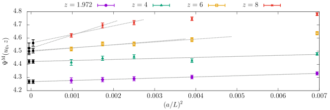
Figure 1: Continuum extrapolation of the massive coupling $\Psi^{\mathrm{M}}(u_{0},z)$. We apply two cuts $(aM)^{2}<1/8,1/4$ in order to estimate the systematic uncertainty.

III.2 Numerical computation

We fix a convenient value

$$[\bar{g}^{(3)}_{\mathrm{GF}}(\mu_{\mathrm{dec}})]^{2}=3.95\equiv u_{0}\,.$$ (20)

With the non-perturbative $\beta$-function of Dalla Brida et al. (2017) and the relation to the physical scale $\mu_{\rm phys}$ of Bruno et al. (2017a, b) we deduce

$$\mu_{\rm dec}=789(15)\,{\rm MeV}\,.$$ (21)

For this choice, the bare parameters, $\tilde{g}_{0}^{2},\,am_{0}=am_{\rm crit}(\tilde{g}_{0}^{2})$ are known rather precisely for several resolutions $L/a$  Fritzsch et al. (2018a), see Table 1.

In order to switch to massive quarks of a given RGI mass, $M=z/L$, we need to know $am_{\rm q}$ which is the solution of

$$z=\frac{L}{a}\,\frac{M}{\kern 1.0pt\overline{\kern-1.0ptm\kern-1.0pt}\kern 1.0pt(\mu_{\mathrm{dec}})}\,Z_{\rm m}(\tilde{g}_{0},a/L)\cdot(1+b_{\mathrm{m}}(\tilde{g}_{0})\,am_{\rm q})\,am_{\rm q}\,,$$ (22)

where $Z_{\rm m}$ is the renormalization factor in the SF scheme employed in  Campos et al. (2018) at scale $\mu_{\mathrm{dec}}=1/L$, the ratio $\frac{M}{\kern 1.0pt\overline{\kern-1.0ptm\kern-1.0pt}\kern 1.0pt(\mu_{\mathrm{dec}})}=1.474(11)$ in the same scheme is derived from the results of Campos et al. (2018), and the term $b_{\mathrm{m}}\,am_{\rm q}$ removes the discretisation effects of ${\rm O}(aM)$. We have computed $Z_{\rm m},\,b_{\mathrm{m}}$, listed in table 1, by dedicated simulations Dalla Brida et al. .

As indicated above, the switch to massive quarks is accompanied by the switch to $\bar{g}_{\mathrm{GFT}}$ in order to suppress linear $1/M$ terms: we evaluate

$$\Psi^{\mathrm{M}}(u_{0},z) = \left[\bar{g}_{\mathrm{GFT}}^{(3)}(\mu_{\mathrm{dec}},M)\right]^{2}_{[\bar{g}_{\mathrm{GF}}^{(3)}(\mu_{\mathrm{dec}})]^{2}=u_{0}}\,,$$

$$z=M/\mu_{\mathrm{dec}}\,.$$

Here, with bare mass $am_{0}$ set as explained, the condition $[\bar{g}_{\mathrm{GF}}^{(3)}(\mu_{\mathrm{dec}})]^{2}=u_{0}$ fixes $\tilde{g}_{0}^{2}$ to the values in table 1.

$L/a$	$6/\tilde{g}_{0}^{2}$	$\;am_{\rm crit}(\tilde{g}_{0}^{2})$	$\;\;\;\bar{g}^{2}_{\mathrm{GF}}$	$\;\;Z_{\rm m}$	$\;\;\;b_{\mathrm{m}}$
12	4.3020	$-0.3234(3)$	3.9533(59)	1.691(7)	$-0.43(3)$
16	4.4662	$-0.3129(2)$	3.9496(77)	1.726(8)	$-0.50(3)$
20	4.5997	$-0.3043(3)$	3.9648(97)	1.741(10)	$-0.48(4)$
24	4.7141	$-0.2969(1)$	3.959(50)	1.770(11)	$-0.51(2)$
32	4.90	$-0.28543(4)$	3.949(11)	1.814(16)	$-0.63(5)$

Table 1: At each $L/a$ the bare coupling $\beta=6/\tilde{g}_{0}^{2}$ and the bare mass $am_{0}=am_{\rm crit}$ are fixed to have constant coupling, eq. (20), and vanishing quark mass Fritzsch et al. (2018a, b), and $Z_{\rm m},b_{\mathrm{m}}$ are determined by simulations with different $am_{\rm q}$ at fixed $\tilde{g}_{0}$ Dalla Brida et al. .

We repeat the exercise for $z=1.972,4,6,8$, which correspond to $M\approx 1.6,3.2,4.7,6.3$ GeV.

It is left to perform continuum extrapolations of the function $\Psi^{\mathrm{M}}(u_{0},z)$, as illustrated in figure 1. They become more challenging at large values of $z$. We explore the systematics by imposing two mass cuts $(aM)^{2}<1/8,\,1/4$ and find compatible results, with the results with $(aM)^{2}<1/8$ having significantly larger errors, at large values of $M$, where few points are left after the cut. We take the extrapolations using $(aM)^{2}<1/8$ as our best estimates of the continuum values of $\Psi^{\mathrm{M}}(u_{0},z)$ (see second column of table 2).

The precise non-perturbative $\beta$-function $\beta_{\mathrm{GF}}^{(0)}$ of Ref. Dalla Brida and Ramos (2019) determines $\varphi_{\mathrm{GF}}^{(0)}(\bar{g}_{\mathrm{GF}})$ in the relevant range of $\bar{g}_{\mathrm{GF}}^{2}\gtrsim 4$. We connect to it from the scheme $\mathrm{GFT}$ by extra simulations, which evaluate $\bar{g}_{\mathrm{GFT}}^{(0)}(\mu)$ at the same parameters $g_{0}^{2},L/a$ where $\bar{g}_{\mathrm{GF}}^{(0)}(\mu)$ is known. After continuum extrapolation of those data with $L/a=12,16,20,24$ we find for $3.8\leq[\bar{g}_{\mathrm{GFT}}^{(0)}]^{2}\leq 5.8$ Dalla Brida et al.

$$[\bar{g}_{\mathrm{GF}}^{(0)}]^{-2}-[\bar{g}_{\mathrm{GFT}}^{(0)}]^{-2}=p_{0}+p_{1}[\bar{g}_{\mathrm{GFT}}^{(0)}]^{2}+p_{2}[\bar{g}_{\mathrm{GFT}}^{(0)}]^{4}\pm 7\times 10^{-4}\,,$$

with $(p_{0},p_{1},p_{2})=(2.886,-0.510,0.056)\times 10^{-2}$. For each of the values $\Psi^{\mathrm{M}}$ in table 2 we obtain $u_{\mathrm{M}}=[\bar{g}_{\mathrm{GF}}^{(0)}]^{2}$ from $[\bar{g}_{\mathrm{GFT}}^{(0)}]^{2}=\Psi^{\mathrm{M}}$, insert into eq. (11) (with scheme $s=\mathrm{GF}$) and solve (numerically) for $\rho$. The table includes $\Lambda_{\rm\overline{MS\kern-0.35002pt}\kern 0.35002pt}^{(3)}$ as well as the influence of the last known term of the series eq. (4) which demonstrates that perturbative uncertainties are negligible.

At present we have used a relatively modest amount of computer time. Our largest lattice is just $64\times 32^{3}$. A significant improvement, simulating lattice spacings twice finer, is possible with current computing power.

$z$	$\Psi^{\mathrm{M}}$	$\Lambda^{(0)}_{\overline{\rm MS}}/{\mu_{\rm dec}}$	$\frac{1}{P(M/\Lambda)}$	$\Lambda^{(3)}_{\overline{\rm MS}}$ [MeV]	$\Delta_{4}$ [MeV]
1.972	4.268(13)	0.689(11)	0.8000(48)	434(12)	2.0
4.0	4.421(13)	0.725(11)	0.6865(28)	393(11)	0.7
6.0	4.499(26)	0.743(13)	0.6283(26)	368(10)	0.4
8.0	4.523(40)	0.749(14)	0.5889(27)	348(11)	0.3
$\infty$	FLAG19 (lattice) Aoki et al. (2019)			343(12)

Table 2: Results for the massive coupling $\Psi^{\mathrm{M}}(u_{0},z)$ at different values of $M$ and fixed $\mu_{\rm dec}=789(15)$ MeV. The perturbative factor $P(M/\Lambda)$ is determined with five-loop running and including $c_{l\leq 4}$ in eq. (4). $\Delta_{4}$ shows the effect of $c_{4}$ in $\Lambda_{\rm\overline{MS\kern-0.31502pt}\kern 0.31502pt}^{(3)}$. The effect of $c_{3}$ is larger by a factor 1.5 (for $z=1.972$) to 3 (for $z=8$).

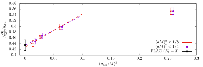
Figure 2: Values for $\rho$ determined from the decoupling relation. As $z=M/\mu_{\rm dec}$ gets larger, the approximations for $\rho=\Lambda_{\rm\overline{MS\kern-0.35002pt}\kern 0.35002pt}/\mu_{\mathrm{dec}}$ approach the FLAG result for $\Lambda^{(3)}_{\rm\overline{MS\kern-0.35002pt}\kern 0.35002pt}$ in units of $\mu_{\mathrm{dec}}=789(15)~{}{\rm MeV}$ Aoki et al. (2019). The dashed lines illustrate possible extrapolations $M\to\infty$ (cf. Eq. (1)). A significant part of the errors at finite $M$ is due to the Yang-Mills theory and may be reduced further.

III.3 Results

According to Eq. (1), the values obtained for $\Lambda^{(3)}_{\overline{\rm MS}}$ approach the true non-perturbative value as $M\to\infty$. We demonstrate this property in the plot of $\rho$, Fig. 2. While we see power corrections, these are small and the point with $M\approx 6$ GeV is in agreement with the known number from Bruno et al. (2017a) as well as with the FLAG average Aoki et al. (2019). Rough extrapolations to the limit $M\to\infty$ seem to make the agreement even better. This limit should be studied with even higher precision in the future.

IV Conclusions

In this letter we propose a new strategy to determine the strong coupling. It requires the determination of a renormalized coupling in an unphysical setup with degenerate massive quarks at some low energy scale. The second ingredient is the determination of the $\Lambda$-parameter in units of the low energy scale in the pure gauge theory defined in terms of the same coupling. As we have shown, there is a clear advantage: the essential part of the multi-scale problem (i.e. the determination of the $\Lambda$-parameter) is done without fermions. The remaining problem, namely the limit of large $M$ can be reached by two observations. First it is known that with a mass $M$ of a few GeV, the perturbative prediction for $P$ is very accurate Herren and Steinhauser (2018); Athenodorou et al. (2019). Second we presented a finite volume strategy which allows to reach masses of several GeV and presented clear evidence that the remaining power corrections are small. The result is in good agreement with the more standard step scaling approach, but promises a higher precision. We note again that we only invested a rather modest numerical effort. The limits $a\to 0$ at fixed $M$ and $M\to\infty$ can be much improved. With more work our new strategy will lead to a substantial reduction of the uncertainty in $\alpha_{s}$. As mentioned, other definitions of the finite volume coupling with other boundary conditions may be chosen.

There is even a more direct approach, simply using $t_{0}$ Lüscher (2010),

$$[\Lambda_{\rm\overline{MS\kern-0.35002pt}\kern 0.35002pt}\sqrt{t_{0}(M)}]^{(N_{\mathrm{f}})}\;P\left(\frac{M}{\Lambda_{\rm\overline{MS\kern-0.35002pt}\kern 0.35002pt}^{(N_{\mathrm{f}})}}\right)=[\Lambda_{\rm\overline{MS\kern-0.35002pt}\kern 0.35002pt}\sqrt{t_{0}}]^{(0)}+{\rm O}(M^{-2})\,,$$

or a different low energy scale (see also Bruno et al. (2015a); Athenodorou et al. (2019)). This only requires to determine such a gluonic scale with at least three degenerate massive quarks. Together with a determination of the pure gauge $\Lambda$-parameter in units of the same scale, this simple strategy could possibly provide a precise determination of the strong coupling. Controlling discretization errors, power corrections and perturbative corrections at the same time will require compromises but is worth exploring.

The idea presented here can easily be extended to other RGI quantities. A clear case is the determination of quark masses. On the other hand, four fermion operators require an investigation from the start, exploring both perturbative and power corrections.