Competition of trivial and topological phases in patterned graphene based heterostructures

Abstract

We explore the effect of mechanical strain on the electronic spectrum of patterned graphene based heterostructures. We focus on the competition of Kekulé-O type distortion favoring a trivial phase and commensurate Kane-Mele type spin-orbit coupling generating a topological phase. We derive a simple low-energy Dirac Hamiltonian incorporating the two gap promoting mechanisms and include terms corresponding to uniaxial strain. The derived effective model explains previous ab initio results through a simple physical picture. We show that while the trivial gap is sensitive to mechanical distortions, the topological gap stays resilient.

I Introduction

Spin-orbitronics is a promising new paradigm of nano-electronics that utilizes the coupling of spin and orbital degrees of freedom of charge carriers [1, 2], enabling the non-magnetic control of spin currents. The exceptionally long spin dephasing time makes graphene an ideal template material for spintronics applications [3, 4, 5, 6]. Kekulé type patterned bond texture has potentially a dramatic impact on the electronic spectrum of graphene [7, 8, 9, 10]. Specifically Kekulé-O type distortion scatters carriers between the two momentum space valleys of graphene resulting in the appearance of a band gap [9]. Mechanical distortions have also a considerable effect on the electronic states of graphene. Recently several experimental groups reported the controlled manipulation of strain fields in graphene based heterostroctures [11, 12, 13, 14, 15, 16]. Andrade and coworkers have recently studied the effect of mechanical strain on the spectrum of Kekulé patterned samples [17]. They showed that strain substantially influences the gap generated due to a Kekulé-O pattern. As strain increases the gap closes pushing the sample from an insulator to a semimetal. Crucially these previous studies did not consider other gap generation mechanisms which may arise in samples compatible with Kekulé-O texture. In our previous works we showed that in graphene based heterostructures, utilizing ternary bismuth tellurohalides, Kekulé distortion is accompanied by strong induced spin-orbit interaction (SOI) [18, 19]. In these structures a competition between two gap generation mechanisms arise. On the one hand Kekulé-O texture favors a trivial band gap, while the induced spin-orbit interaction drives a topological Kane-Mele type gap [20]. Consequently it has been found that mechanical distortions can drive the system from a trivial insulator to a topological phase.

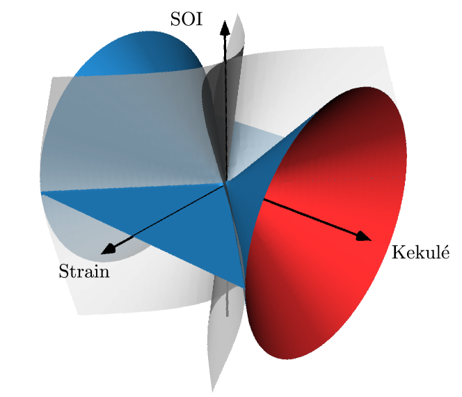
Figure 1: The phase diagram of the considered model based on Eq. (3) and the discussion below. Parameter set from the inside of the cones depicts a trivial gap, while outside of the cones the system is topological. The band gap is closed on the solid surfaces. Between the gray opaque shape and the cones the gap is located at zero momentum, everywhere else it is shifted away to a finite value.
(color online)

In this manuscript we present a simple effective low-energy Dirac model that captures the essence of this mechanically controlled topological quantum phase transition. Our findings are summarized in a three-dimensional phase diagram extracted from the investigated model as depicted in Fig. 1. Inside the cones the Kekulé distortion outpowers the spin-orbit coupling, therefore the system is a trivial insulator, while outside of the cones, spin-orbit coupling is dominant, subsequently the gap is topological. Solid surfaces denote the phase boundaries, where the gap is closed and the system is metallic. We first introduce the low-energy Hamiltonian and then determine the low-energy spectrum. Based on analytical properties of the spectrum we elucidate how mechanical distortions influence the competition of the two types of gap promoting effects. In Appendix A we give a detailed derivation of the low-energy Hamiltonian based on a tight-binding model inspired by previous first principles calculations. In Appendix B we outline the procedure we used to classify the topological phases of the investigated system.

II Model and Results

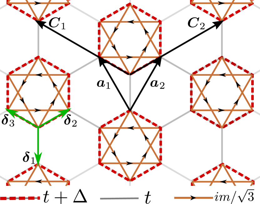
Figure 2: Schematic structure of the unstrained model. The pale gray hexagons represent the unadulterated graphene substrate. Each pale gray bond corresponds to a hopping amplitude $t$. The red dashed lines denote the Kekulé-O type bond alteration with a characteristic strength of $\Delta$. Each gray bond with a red dashed line on top corresponds to a hopping amplitude $t+\Delta$. Brown lines connecting next-nearest neighbor sites symbolize the induced Kane-Mele type spin-orbit coupling. Each brown line corresponds to a spin dependent hopping amplitude ${i}m$, in the direction of the arrows. For more details see the Appendix.
(color online)

Let us consider the tight-binding model of a patterned graphene lattice as depicted in Fig. 2. Each first nearest neighbor bond carries a hopping amplitude of $t$. Kekulé-O distortion is taken into account through an additional $\Delta$ hopping term supplementing each bond around every third hexagon. These terms will be responsible for opening a trivial gap [9]. On the same hexagons the Kekulé-O distortion is active we also introduce a next-nearest neighbour spin dependent hopping. For spin up electrons this corresponds to a hopping amplitude ${i}m$ in the direction of the bond vectors denoted by arrows, while $-{i}m$ for spin down particles. This term, adopted from the Kane-Mele model, promotes a topological gap [20]. Also note that the considered spin-orbit coupling preserves the $z$ component of the spin operator, thus the up and down spin orientations can effectively be treated separately. Besides the considered bond texture discussed above we also incorporate a uniaxial in-plane strain in our description. We take into account the linear distortion of the lattice vectors and the exponential renormalization of all hopping terms.

Since the considered model is diagonal in the spin degree of freedom its $\mathbb{Z}_{2}$ topological index, characterizing time reversal symmetric systems, is given by the parity of the total Chern number calculated for one spin component of the occupied bands [21, 22, 23]. In Appendix B we briefly summarize the procedure to obtain the Chern number of the investigated system.

The following simplified low-energy Hamiltonian captures the most important aspects of the electronic structure in the vicinity of the distorted Dirac cones of graphene (for derivation of the model see in Appendix A):

$$\begin{split}H_{\mathrm{eff}}&=-v\left[\bm{\sigma}\bm{A}\otimes\tau_{z}\otimes s_{0}+\bm{\sigma}\bm{k}\otimes\tau_{0}\otimes s_{0}\right]\\ &+\Delta\sigma_{z}\otimes\tau_{x}\otimes s_{0}-m\sigma_{z}\otimes\tau_{0}\otimes s_{z},\end{split}$$ (1)

where $\bm{k}$ is the momentum, $v=3a_{\mathrm{cc}}/2t$ is the Fermi velocity (in units of $\hbar$) with $a_{\mathrm{cc}}=1.42\,\mathrm{\AA}$ the equilibrium carbon-carbon bond distance [24]. The $\bm{\sigma}=(\sigma_{x},\sigma_{y})$, $\tau_{i}$ and $s_{i}$ are the Pauli matrices. $\sigma_{i}$ are acting on the sublattice, $\tau_{i}$ on the valley degree of freedom while $s_{i}$ act on the real spin.The pseudovector potential $\bm{A}$ describes mechanical distortions, specifically for the case of uniaxial in-plane strain its components are [25, 26, 27, 28]:

$$\bm{A}=\frac{\beta}{2a_{\mathrm{cc}}}\varepsilon\left(1+\rho\right)\left(\begin{array}[]{r}\cos 2\theta\\ -\sin 2\theta\end{array}\right),$$ (2)

where $\beta\approx 3$ is the Grüneisen parameter [29, 30, 31] that modulates the hopping terms of the tight-binding model as strain changes the intercarbon distance due to lattice deformations, $\varepsilon$ is the magnitude of the distortion, $\rho$ is the Poisson ratio, estimated to be $\rho\approx 0.165$ for graphene [32, 33, 34] while $\theta$ is the angular direction of the strain with respect to the $x$ axis.

Since Hamiltonian (1) is diagonal in the proper spin degree of freedom each spin species can be treated separately. Diagonalizing (1) yields the same spectrum for both spin orientations:

$$E\left(\bm{k}\right)=\pm\sqrt{\xi^{2}+\Delta^{2}+v^{2}|\bm{k}|^{2}+m^{2}\pm 2\sqrt{\xi^{2}\Delta^{2}+\left(v^{2}\bm{A}\cdot\bm{k}\right)^{2}+\Delta^{2}m^{2}}},$$ (3)

where we introduce

$$\xi=v\frac{\beta}{2a_{\mathrm{cc}}}\varepsilon\left(1+\rho\right).$$ (4)

The low-energy spectrum of the considered tight-binding model (42) and the effective Dirac Hamiltonian (1) for various model parameters is shown in Fig. 3. In the first row we show a clean graphene sample under strain. As the magnitude of the mechanical distortion increases the two Dirac cones shift apart. In the second row a trivial gap opened by Kekulé pattern is closed by an ever increasing strain driving the system into a semimetallic phase. On the contrary, as it can be observed in the third row the topological gap opened by the Kane-Mele term is insensitive to the strength of distortion. In the last row both gap generation mechanism are active and $\Delta>m$ resulting in a trivial gap for the unstrained case. As strain is increased the gap is closed and reopened but now with a topological flavor.

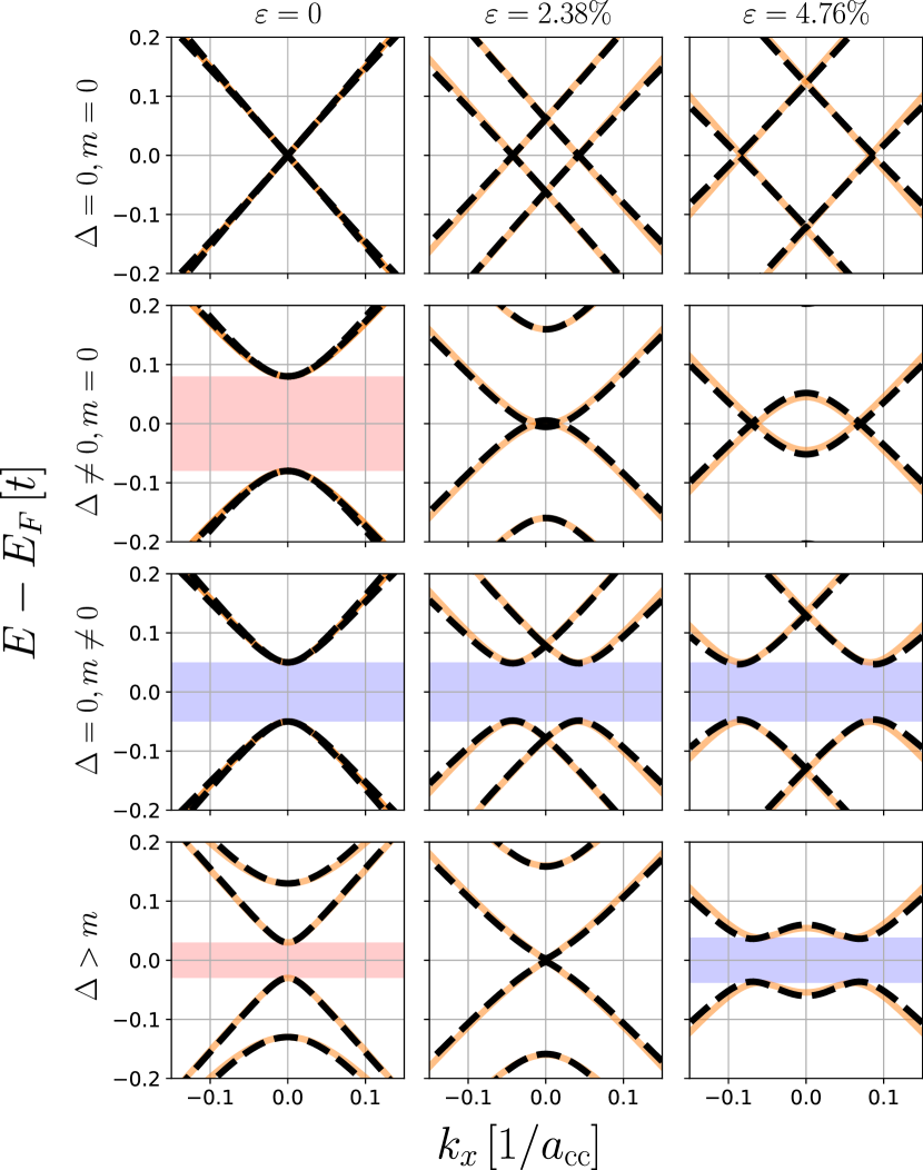
Figure 3: The low-energy spectrum of the considered tight-binding model (42), denoted by solid orange lines, and the effective Dirac Hamiltonian (1), depicted with dashed black lines, for various parameters. Topological gaps are indicated by blue opaque coloring, while trivial gaps are highlighted with red. In all panels $m=0.04t$ and $\Delta=0.08t$ unless indicated otherwise, for all cases $\theta=0$.
(color online)

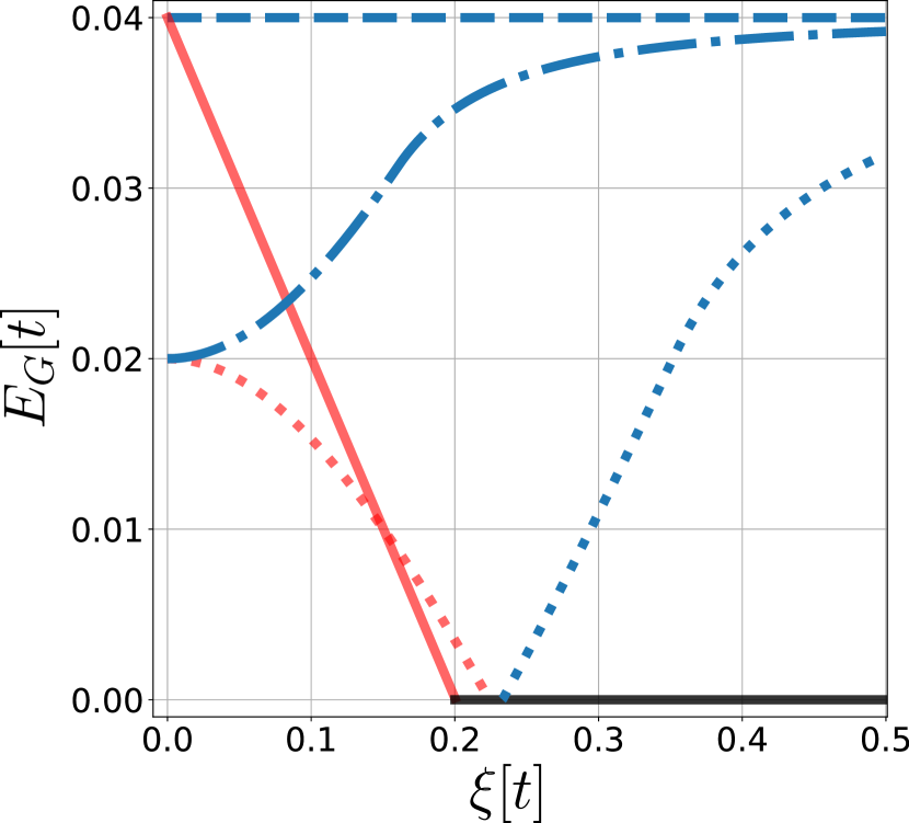
Figure 4: The magnitude of the gap obtained from the effective Dirac Hamiltonian is shown as the function of uniaxial strain for various model parameters. Red color indicates that the gap is trivial, while blue coloring shows that the gap is topological. The dashed line corresponds to $\Delta=0$ and $m=0.04t$. The solid line shows the case when $\Delta=0.04t$ and $m=0$. The dashdotted line was obtained using $\Delta=0.01t$ and $m=0.02t$ while in the case of the dotted curve it was $\Delta=0.03t$ and $m=0.02t$.
(color online)

Analyzing the spectrum, depicted in Fig. 3, the conditions for sustaining a gap can be discerned. We find, that if the applied mechanical distortion is constrained as

$$2\xi^{2}\leq\sqrt{\Delta^{2}\left(\Delta^{2}+4m^{2}\right)}+\Delta^{2},$$ (5)

then the band extrema are at $\bm{k}=(0,0)$ and the magnitude of the gap is

$$E_{\mathrm{G}}=2\sqrt{\xi^{2}+\Delta^{2}+m^{2}-2\sqrt{\xi^{2}\Delta^{2}+\Delta^{2}m^{2}}}.$$ (6)

The gap closes if $\xi=\sqrt{\Delta^{2}-m^{2}}$ at which point valence and conduction band touch at a single point. If condition (5) is unsatisfied the band extrema are shifted to a finite momentum, the magnitude of the gap in this case is:

$$E_{\mathrm{G}}=2m\sqrt{1-\frac{\Delta^{2}}{\xi^{2}}}$$ (7)

We note that the observations made above are insensitive to the direction of strain i.e. $\theta$, similarly to previous results [29, 17].

The impact of strain on the competition between the two topologically distinct phases can be observed in Fig. 4. Here we plot the evolution of the magnitude and character of the gap as the function of the strength of the applied mechanical distortion based on (6) and (7). If only the Kekulé term is active, shown with solid lines, then the gap decreases linearly with increasing strain and once it is closed the system remains gapless. On the other hand if we only keep the next-nearest spin-orbit coupling, indicated by dashed lines, the gap remains constant in the face of ever increasing strain. If $\Delta>m$, shown with dotted lines, the original trivial gap closes and a nontrivial gap opens as strain is increased. For $m>\Delta$, denoted by a dash-dotted line, an initial smaller topological gap is increased by the application of mechanical distortions.

III Conclusion

We studied the effects of uniaxial strain upon the electronic properties of a patterned graphene lattice hosting a Kekulé-O textured bond alternation and a commensurate Kane-Mele type spin-orbit coupling. Based on a tight-binding model we distilled an effective, low-energy Dirac Hamiltonian. Analyzing the spectrum of the model we explored the various gaped phases present in the sample. We found that while the trivial gap favored by the Kekulé-O distortion is destroyed by the strain, the topological gap generated by the considered spin-orbit term remains resilient. This observation can be understood from the following reasoning. The applied mechanical distortion moves the two Dirac cones of graphene from their initial position. The Kekulé term scatters particles between valleys, and hence it can only open a gap if the Dirac cones are aligned. The Kane-Mele term on the other hand does not mix valleys and the gap opened through it is insensitive to the position of the Dirac cones. These findings explain our previous ab initio results [18].

Conflicts of interest

There are no conflicts to declare.

Appendix A

In this Section, we present the derivation of our simplified low-energy Hamiltonian (Eq. (1)). The system of interest is the Kekulé-O distorted graphene lattice hosting next-nearest neighbor Kane-Mele type spin-orbit interaction in the perturbed hexagons (See Fig. 2). To study the impact of mechanical strain on the electronic spectrum, we introduced uniform, planar strain,id est, the strain is position independent. Thus the displacement field of the atoms due to the deformation is given by: $\bm{u}(\tilde{\bm{r}})=\bm{\varepsilon}\cdot\tilde{\bm{r}}$, where $\tilde{\bm{r}}$ is the original position of the cores. After deformation the position of the atoms are $\bm{r}=\tilde{\bm{r}}+\bm{u}(\tilde{\bm{r}})=\left(\bm{I}+\bm{\varepsilon}\right)\tilde{\bm{r}}$, where $\bm{I}$ is the 2$\times$2 identity matrix and the deformation tensor $\bm{\varepsilon}$ can be parametrized as:

$$\bm{\varepsilon}=\varepsilon\left(\begin{array}[]{cc}\mathrm{cos}^{2}\theta-\rho\mathrm{sin^{2}\theta}&\left(1+\rho\right)\mathrm{cos}\theta\mathrm{sin}\theta\\ \left(1+\rho\right)\mathrm{cos}\theta\mathrm{sin}\theta&\mathrm{sin^{2}\theta}-\rho\mathrm{cos}^{2}\theta\end{array}\right),$$ (8)

where $\varepsilon$ is the magnitude of the applied strain, $\theta$ is its angular direction, with respect to the $x$ axis and $\rho$ is the Poisson ratio, which relates the transverse strain to the axial component (estimated to be $\rho=0.165$ for graphene).

We applied the above outlined formalism to include strain in our model, which can be formulated as:

$$\hat{H}=\left(\begin{array}[]{cc}\hat{h}_{\uparrow}&0\\ 0&\hat{h}_{\downarrow}\end{array}\right).$$ (9)

Since Hamiltonian (9) is diagonal in the proper spin degree of freedom [20] each spin species can be treated separately:

$$\hat{h}_{\uparrow/\downarrow}=\hat{H}_{\mathrm{Gr}}+\hat{H}_{\mathrm{Kek}}\pm\hat{H}_{\mathrm{SOI}},$$ (10)

where $\hat{H}_{\mathrm{Gr}}$ describes the pristine graphene, $\hat{H}_{\mathrm{Kek}}$ is the Hamiltonian of the Kekulé distortion and $\hat{H}_{\mathrm{SOI}}$ incorporates the patterned next-nearest-neighbor spin-orbit interaction.

First let us consider the clean, pristine graphene. The structure of graphene is defined by a unit cell consisting of two equivalent atoms A and B with one $\pi$ orbital per carbon atom considered. The lattice is spanned by the lattice vectors: $\tilde{\bm{a}}_{1,2}=a_{\mathrm{cc}}\frac{1}{2}\left(\mp\sqrt{3},\,3\right)$, where ${a_{\mathrm{cc}}}\approx 1.42\,\mathrm{\AA}$ is the unperturbed carbon-carbon distance in the lattice. We define single particle states situated on sublattice $\alpha=A\,\mathrm{or}\,B$ as:

$$\left|\alpha,\underline{m}\cdot\underline{\bm{a}}\right\rangle=\left|\alpha\right\rangle\left|\underline{m}\cdot\underline{\bm{a}}\right\rangle$$ (11)

where $\underline{m}\cdot\underline{\bm{a}}$ runs over the atomic positions as $\underline{m}\cdot\underline{\bm{a}}=m_{1}\bm{a}_{1}+m_{2}\bm{a}_{2}$ with $m_{1}$ and $m_{2}$ being integers. With this notation the tight-binding Hamiltonian for strained graphene in real space is given by:

$$\begin{split}\hat{H}_{\mathrm{Gr}}=t\sum_{\underline{m}}&d_{1}\left|B,\underline{m}\cdot\underline{\bm{a}}\right\rangle\left\langle A,\underline{m}\cdot\underline{\bm{a}}\right|\\ +&d_{2}\left|B,\underline{m}\cdot\underline{\bm{a}}\right\rangle\left\langle A,\underline{m}\cdot\underline{\bm{a}}+\bm{a}_{1}\right|\\ +&d_{3}\left|B,\underline{m}\cdot\underline{\bm{a}}\right\rangle\left\langle A,\underline{m}\cdot\underline{\bm{a}}+\bm{a}_{2}\right|+\text{h.c.},\end{split}$$ (12)

where $t\approx 2.7\,\mathrm{eV}$ is the hopping parameter of unstrained graphene and the $d_{i}$ factors describe the strain. Hence the overlap integrals depend on the actual position of the atoms, the effect of strain on the hopping terms can be taken into account with the following factors [35, 36, 4]:

$$d_{i}=\mathrm{e}^{-\beta\left(\frac{|\bm{\delta}_{i}|}{a_{\mathrm{cc}}}-1\right)},\qquad i=1,2,3,$$ (13)

where $\beta$ is the Grüneisen parameter (estimated to be $\beta\approx 3$ for graphene) and $\bm{\delta}_{i}$ are the bonding vectors pointing to one of the three nearest-neighbor sites at a given $\bm{r}$, as shown in Fig. 2, $\tilde{\bm{\delta}}_{1}=a_{\mathrm{cc}}\left(0,-1\right),\tilde{\bm{\delta}}_{2}=a_{\mathrm{cc}}/2\left(\sqrt{3},1\right)$, $\tilde{\bm{\delta}}_{3}=a_{\mathrm{cc}}/2\left(-\sqrt{3},1\right)$.

In the next step, let us introduce the Kekulé-O distortion. The texture of the ordering is visualized in Fig. 2. The periodicity of the pattern differs from the pristine graphene and can be written as: $\bm{C}_{1}=2\bm{a}_{1}-\bm{a}_{2}$ and $\bm{C}_{2}=-\bm{a}_{1}+2\bm{a}_{2}.$ We can formulate the Hamiltonian of the Kekulé-O texture in real space as:

$$\begin{split}\hat{H}_{\mathrm{KeK}}&={\Delta}\sum_{\underline{M}}d_{2}\left|B,\underline{M}\cdot\underline{\bm{C}}\right\rangle\left\langle A,\underline{M}\cdot\underline{\bm{C}}+\bm{a}_{2}\right|\\ &+d_{1}\left|B,\underline{M}\cdot\underline{\bm{C}}+\bm{a}_{2}\right\rangle\left\langle A,\underline{M}\cdot\underline{\bm{C}}+\bm{a}_{2}\right|\\ &+d_{3}\left|B,\underline{M}\cdot\underline{\bm{C}}+\bm{a}_{2}\right\rangle\left\langle A,\underline{M}\cdot\underline{\bm{C}}+\bm{a}_{2}+\bm{a}_{1}\right|\\ &+d_{2}\left|B,\underline{M}\cdot\underline{\bm{C}}+\bm{a}_{1}\right\rangle\left\langle A,\underline{M}\cdot\underline{\bm{C}}+\bm{a}_{2}+\bm{a}_{1}\right|\\ &+d_{1}\left|B,\underline{M}\cdot\underline{\bm{C}}+\bm{a}_{1}\right\rangle\left\langle A,\underline{M}\cdot\underline{\bm{C}}+\bm{a}_{1}\right|\\ &+d_{3}\left|B,\underline{M}\cdot\underline{\bm{C}}\right\rangle\left\langle A,\underline{M}\cdot\underline{\bm{C}}+\bm{a}_{1}\right|+\text{h.c.},\end{split}$$ (14)

where $\underline{M}\cdot\underline{\bm{C}}$ runs over the atomic positions as $\underline{M}\cdot\underline{\bm{C}}=M_{1}\bm{C}_{1}+M_{2}\bm{C}_{2}$ with $M_{1}$ and $M_{2}$ being integers and $\Delta$ is the strength of the Kekulé distortion. (We note that our definiton of $\Delta$ is different from [17]).

The last part of our model is the next-nearest neighbor spin-orbit interaction. In order to preserve time-reversal symmetry we write the SOI term as $im/\sqrt{3}$, where $m$ is the strength of the interaction and has a real value. We introduced an extra $1/\sqrt{3}$ factor in the magnitude of the interaction, which will be convenient later. The real space periodicity of this term is the same as in the case of the Kekulé texture:

$$\begin{split}\hat{H}_{\mathrm{SOI}}&=\frac{im}{\sqrt{3}}\sum_{\underline{M}}d_{5}\left|B,\underline{M}\cdot\underline{\bm{C}}+\bm{a}_{2}\right\rangle\left\langle B,\underline{M}\cdot\underline{\bm{C}}\right|\\ &+d_{4}\left|B,\underline{M}\cdot\underline{\bm{C}}\right\rangle\left\langle B,\underline{M}\cdot\underline{\bm{C}}+\bm{a}_{1}\right|\\ &+d_{6}\left|B,\underline{M}\cdot\underline{\bm{C}}+\bm{a}_{1}\right\rangle\left\langle B,\underline{M}\cdot\underline{\bm{C}}+\bm{a}_{2}\right|\\ &+d_{5}\left|A,\underline{M}\cdot\underline{\bm{C}}+\bm{a}_{1}\right\rangle\left\langle A,\underline{M}\cdot\underline{\bm{C}}+\bm{a}_{1}+\bm{a}_{2}\right|\\ &+d_{4}\left|A,\underline{M}\cdot\underline{\bm{C}}+\bm{a}_{1}+\bm{a}_{2}\right\rangle\left\langle A,\underline{M}\cdot\underline{\bm{C}}+\bm{a}_{2}\right|\\ &+d_{6}\left|A,\underline{M}\cdot\underline{\bm{C}}+\bm{a}_{2}\right\rangle\left\langle A,\underline{M}\cdot\underline{\bm{C}}+\bm{a}_{1}\right|+\text{h.c.}.\end{split}$$ (15)

The factors ($d_{4,5,6}$) of the hopping terms have a different form corresponding to the next-nearest neigbor bonding vectors:

$$d_{4}=\mathrm{e}^{-\beta\left(\frac{|\bm{a}_{1}|}{\sqrt{3}a_{\mathrm{cc}}}-1\right)},$$ (16)

$$d_{5}=\mathrm{e}^{-\beta\left(\frac{|\bm{a}_{2}|}{\sqrt{3}a_{\mathrm{cc}}}-1\right)},$$

$$d_{6}=\mathrm{e}^{-\beta\left(\frac{|\bm{a}_{1}-\bm{a}_{2}|}{\sqrt{3}a_{\mathrm{cc}}}-1\right)}.$$

In order to compute the dispersion relation we must take the Fourier transform of our Hamiltonian (9). We define the transformation via the following relations [37]:

$$\left|B,\underline{m}\cdot\underline{\bm{a}}\right\rangle=\frac{1}{\sqrt{N}}\sum_{\bm{k}}\mathrm{e}^{i\bm{k}\underline{m}\cdot\underline{\bm{a}}}\left|B,\bm{k}\right\rangle,$$ (17)

$$\left|A,\underline{m}\cdot\underline{\bm{a}}\right\rangle=\frac{1}{\sqrt{N}}\sum_{\bm{k}}\mathrm{e}^{i\bm{k}\left(\underline{m}\cdot\underline{\bm{a}}+\bm{\delta}_{1}\right)}\left|A,\bm{k}\right\rangle,$$

where $N$ is the number of the unit cells.

While calculating the Hamiltonian in $\bm{k}$-space is in principle straightforward, we impart a couple of remarks. Using the definition in Eq. (17) we perform the Fourier transformation of the first term in Eq. (12).

$$\sum_{\underline{m}}d_{1}\left|B,\underline{m}\cdot\underline{\bm{a}}\right\rangle\left\langle A,\underline{m}\cdot\underline{\bm{a}}\right|$$ (18)

$$=\frac{d_{1}}{N}\sum_{\underline{m}}\sum_{\bm{k}^{\prime},\bm{k}}\mathrm{e}^{i\bm{k}\underline{m}\cdot\underline{\bm{a}}}\mathrm{e}^{-i\bm{k}^{\prime}\left(\underline{m}\cdot\underline{\bm{a}}+\bm{\delta}_{1}\right)}\left|B,\bm{k}\right\rangle\left\langle A,\bm{k}^{\prime}\right|$$

$$=\frac{d_{1}}{N}\sum_{\underline{m}}\sum_{\bm{k}^{\prime},\bm{k}}\mathrm{e}^{i\underline{m}\cdot\underline{\bm{a}}\left(\bm{k}-\bm{k}^{\prime}\right)}\mathrm{e}^{-i\bm{k}^{\prime}\bm{\delta}_{1}}\left|B,\bm{k}\right\rangle\left\langle A,\bm{k}^{\prime}\right|.$$

Examine more closely the following term:

$$\sum_{\underline{m}}\mathrm{e}^{i\underline{m}\cdot\underline{\bm{a}}\left(\bm{k}-\bm{k}^{\prime}\right)}=\sum_{m_{1}=1}^{n_{1}}\sum_{m_{2}=1}^{n_{2}}\mathrm{e}^{i\left(m_{1}\bm{a}_{1}+m_{2}\bm{a}_{2}\right)\Delta\bm{k}},$$ (19)

where $n_{1}\cdot n_{2}=N$ and $\Delta\bm{k}=\bm{k}-\bm{k}^{\prime}$. We rewrite the $\Delta\bm{k}$ term as a linear combination of the reciprocal lattice vectors: $\Delta\bm{k}=\Delta k_{1}\cdot\bm{b}_{1}+\Delta k_{2}\cdot\bm{b}_{2}$, where $\Delta k_{i}=\frac{l}{n_{i}}$ with $l=0...n_{i}-1$. Plugging this back to Eq. (19):

$$\sum_{\underline{m}}\mathrm{e}^{i\underline{m}\cdot\underline{\bm{a}}\left(\bm{k}-\bm{k}^{\prime}\right)}=\sum_{m_{1}=1}^{n_{1}}\mathrm{e}^{2\pi im_{1}\Delta k_{1}}\sum_{m_{2}=1}^{n_{2}}\mathrm{e}^{2\pi im_{2}\Delta k_{2}}$$

$$=n_{1}\delta_{\Delta k_{1},0}\cdot n_{2}\delta_{\Delta k_{2},0},$$ (20)

where $\delta_{i,j}$ is the Kronecker symbol [38, 39]. Applying this to Eq. (18) we get that

$$\sum_{\underline{m}}d_{1}\left|B,\underline{m}\cdot\underline{\bm{a}}\right\rangle\left\langle A,\underline{m}\cdot\underline{\bm{a}}\right|=d_{1}\sum_{\bm{k}}\mathrm{e}^{-i\bm{k}\bm{\delta}_{1}}\left|B,\bm{k}\right\rangle\left\langle A,\bm{k}\right|.$$ (21)

The Fourier transformation of the terms with different periodicity must be done in the same manner. We show the first term of Eq. (14) as an example:

$$\sum_{M_{1},M_{2}}\left|B,M_{1}\bm{C}_{1}+M_{2}\bm{C}_{2}\right\rangle\left\langle A,M_{1}\bm{C}_{1}+M_{2}\bm{C}_{2}+\bm{a}_{2}\right|$$ (22)

$$=\frac{1}{N}\sum_{\bm{k},\bm{k}^{\prime}}\sum_{M_{1},M_{2}}\mathrm{e}^{i\bm{k}\left(M_{1}\left(2\bm{a}_{1}-\bm{a}_{2}\right)+M_{2}\left(2\bm{a}_{2}-\bm{a}_{1}\right)\right)}\left|B,\bm{k}\right\rangle\mathrm{e}^{-i\bm{k}^{\prime}\left(M_{1}\left(2\bm{a}_{1}-\bm{a}_{2}\right)+M_{2}\left(2\bm{a}_{2}-\bm{a}_{1}\right)+\bm{a}_{2}\right)}\mathrm{e}^{-i\bm{k}^{\prime}\bm{\delta}_{1}}\left\langle A,\bm{k}^{\prime}\right|$$

$$=\frac{1}{N}\sum_{\bm{k},\bm{k}^{\prime}}\sum_{M_{1},M_{2}}\left|B,\bm{k}\right\rangle\left\langle A,\bm{k}^{\prime}\right|\mathrm{e}^{-i\left(\bm{k}^{\prime}-\bm{k}\right)\left(M_{1}\left(2\bm{a}_{1}-\bm{a}_{2}\right)+M_{2}\left(2\bm{a}_{2}-\bm{a}_{1}\right)\right)}\mathrm{e}^{-i\bm{k}^{\prime}(\overbrace{\bm{a}_{2}+\bm{\delta}_{1}}^{\bm{\delta}_{2}})}.$$

Summing the terms that depend on $M_{i}$, we get:

$$\sum_{M_{1}=1}^{N_{1}}\sum_{M_{2}=1}^{N_{2}}\mathrm{e}^{-i\left(\bm{k}^{\prime}-\bm{k}\right)\left(M_{1}\left(2\bm{a}_{1}-\bm{a}_{2}\right)+M_{2}\left(2\bm{a}_{2}-\bm{a}_{1}\right)\right)}$$ (23)

where $N_{1}\cdot N_{2}=N/3$ is the number of the larger unit cell respecting the periodicity of the Kekulé pattern. We can rewrite the terms in the exponent as:

$$\footnotesize M_{1}\left(2\bm{a}_{1}-\bm{a}_{2}\right)+M_{2}\left(2\bm{a}_{2}-\bm{a}_{1}\right)=\left(\begin{array}[]{cc}\bm{a}_{1}&\bm{a}_{2}\end{array}\right)\left(\begin{array}[]{rr}2&-1\\ -1&2\end{array}\right)\left(\begin{array}[]{c}M_{1}\\ M_{2}\end{array}\right).$$ (24)

We can do the same expansion in the terms of the reciprocal lattice vectors as we did above:

$$\left(\begin{array}[]{cc}\Delta k_{1}&\Delta k_{2}\end{array}\right)\left(\begin{array}[]{c}\bm{b}_{1}\\ \bm{b}_{2}\end{array}\right)\left(\begin{array}[]{rr}\bm{a}_{1}&\bm{a}_{2}\end{array}\right)\left(\begin{array}[]{rr}2&-1\\ -1&2\end{array}\right)\left(\begin{array}[]{c}M_{1}\\ M_{2}\end{array}\right)$$ (33)

$$=2\pi\left(\begin{array}[]{rr}\Delta k_{1}&\Delta k_{2}\end{array}\right)\left(\begin{array}[]{rr}2&-1\\ -1&2\end{array}\right)\left(\begin{array}[]{c}M_{1}\\ M_{2}\end{array}\right).$$ (39)

If this exponent is a multiple of $2\pi$ then the value of the expression is 1 and 0 otherwise. Which means we can translate the question to a set of linear equations and solve it over the integer numbers keeping in mind the fact that the $\Delta k_{i}$ numbers have a finite set similarly as before. This problem has 3 different solutions: $\bm{k}-\bm{k}^{\prime}=\bm{0},\pm\bm{G}$, where ${\bm{G}=\frac{1}{3}(\bm{b}_{1}-\bm{b}_{2})}$ is the so-called Kekulé wave vector [40, 17]:

$$\sum_{M_{1}=1}^{N_{1}}\sum_{M_{2}=1}^{N_{2}}\mathrm{e}^{-i\left(\bm{k}^{\prime}-\bm{k}\right)\left(M_{1}\left(2\bm{a}_{1}-\bm{a}_{2}\right)+M_{2}\left(2\bm{a}_{2}-\bm{a}_{1}\right)\right)}$$ (40)

$$=\frac{N}{3}\left(\delta_{\bm{k},\bm{k}^{\prime}}+\delta_{\bm{k},\bm{k}^{\prime}\pm\bm{G}}\right).$$

Now we can write down the Fourier transform:

$$\sum_{M_{1},M_{2}}\left|B,M_{1}\bm{C}_{1}+M_{2}\bm{C}_{2}\right\rangle\left\langle A,M_{1}\bm{C}_{1}+M_{2}\bm{C}_{2}+\bm{a}_{2}\right|$$

$$=\frac{1}{3}\sum_{\bm{k}}\left|B,\bm{k}\right\rangle\left\langle A,\bm{k}\right|\mathrm{e}^{-i\bm{k}\bm{\delta}_{2}}+\left|B,\bm{k}\right\rangle\left\langle A,\bm{k}+\bm{G}\right|\mathrm{e}^{-i\left(\bm{k}+\bm{G}\right)\bm{\delta}_{2}}$$

$$+\left|B,\bm{k}\right\rangle\left\langle A,\bm{k}-\bm{G}\right|\mathrm{e}^{-i\left(\bm{k}-\bm{G}\right)\bm{\delta}_{2}}.$$ (41)

Performing the Fourier transformation on every term in the Eq. (10) Hamiltonian in $\bm{k}$-space can be written as: $\hat{h}_{\uparrow/\downarrow}=\sum_{\bm{k}}\underline{\Psi}^{\dagger}_{\bm{k}}H_{\uparrow/\downarrow}(\bm{k})\underline{\Psi}_{\bm{k}}$ with

$$H(\bm{k})_{\uparrow/\downarrow}=\left(\begin{tabular}[]{cc}$\pm\bm{\Omega}$&$\bm{\Gamma}$\\ $\bm{\Gamma}^{\dagger}$&$\mp\bm{\Omega}^{\dagger}$\\ \end{tabular}\right),$$ (42)

where

$$\underline{\Psi}^{\dagger}_{\bm{k}}=\left(\begin{array}[]{cccccc}\left|B\bm{k}\right\rangle&\left|B,\bm{k}+\bm{G}\right\rangle&\left|B,\bm{k}-\bm{G}\right\rangle&\left|A,\bm{k}\right\rangle&\left|A,\bm{k}+\bm{G}\right\rangle&\left|A,\bm{k}-\bm{G}\right\rangle\end{array}\right),$$ (43)

$$\bm{\Gamma}=\left(\begin{tabular}[]{ccc}$\left(t+\frac{2\Delta}{3}\right)s(\bm{k},\bm{0})/2$&$\frac{\Delta}{3}s(\bm{k},\bm{G})$&$\frac{\Delta}{3}s(\bm{k},-\bm{G})$\\ $\frac{\Delta}{3}s(\bm{k}+\bm{G},-\bm{G})$&$\left(t+\frac{2\Delta}{3}\right)s(\bm{k}+\bm{G},\bm{0})/2$&$\frac{\Delta}{3}s(\bm{k}+\bm{G},\bm{G})$\\ $\frac{\Delta}{3}s(\bm{k}-\bm{G},\bm{G})$&$\frac{\Delta}{3}s(\bm{k}-\bm{G},-\bm{G})$&$\left(t+\frac{2\Delta}{3}\right)s(\bm{k}-\bm{G},\bm{0})/2$\\ \end{tabular}\right),$$ (44)

$$\bm{\Omega}=\frac{im}{3\sqrt{3}}\left(\begin{tabular}[]{ccc}$s^{\prime}\left(\bm{k},\bm{0}\right)-s^{\prime*}\left(\bm{k},\bm{0}\right)$&$s^{\prime}\left(\bm{k},\bm{G}\right)-s^{\prime*}\left(\bm{k}+\bm{G},-\bm{G}\right)$&$s^{\prime}\left(\bm{k},-\bm{G}\right)-s^{\prime*}\left(\bm{k}-\bm{G},\bm{G}\right)$\\ $s^{\prime}\left(\bm{k}+\bm{G},-\bm{G}\right)-s^{\prime*}\left(\bm{k},\bm{G}\right)$&$s^{\prime}\left(\bm{k}+\bm{G},\bm{0}\right)-s^{\prime*}\left(\bm{k}+\bm{G},\bm{0}\right)$&$s^{\prime}\left(\bm{k}+\bm{G},\bm{G}\right)-s^{\prime*}\left(\bm{k}-\bm{G},-\bm{G}\right)$\\ $s^{\prime}\left(\bm{k}-\bm{G},\bm{G}\right)-s^{\prime*}\left(\bm{k},-\bm{G}\right)$&$s^{\prime}\left(\bm{k}-\bm{G},-\bm{G}\right)-s^{\prime*}\left(\bm{k}+\bm{G},\bm{G}\right)$&$s^{\prime}\left(\bm{k}-\bm{G},\bm{0}\right)-s^{\prime*}\left(\bm{k}-\bm{G},\bm{0}\right)$\end{tabular}\right).$$ (45)

Here we introduced the following functions:

$$s\left(\bm{k},\bm{p}\right)=d_{1}\mathrm{e}^{-i\bm{k}\left(1+\bm{\varepsilon}\right)\tilde{\bm{\delta}}_{1}}\left(\mathrm{e}^{-i\bm{p}\tilde{\bm{\delta}}_{3}}+\mathrm{e}^{-i\bm{p}\tilde{\bm{\delta}}_{2}}\right)$$ (46)

$$+d_{2}\mathrm{e}^{-i\bm{k}\left(1+\bm{\varepsilon}\right)\tilde{\bm{\delta}}_{2}}\left(\mathrm{e}^{-i\bm{p}\tilde{\bm{\delta}}_{1}}+\mathrm{e}^{-i\bm{p}\tilde{\bm{\delta}}_{2}}\right)$$

$$+d_{3}\mathrm{e}^{-i\bm{k}\left(1+\bm{\varepsilon}\right)\tilde{\bm{\delta}}_{3}}\left(\mathrm{e}^{-i\bm{p}\tilde{\bm{\delta}}_{3}}+\mathrm{e}^{-i\bm{p}\tilde{\bm{\delta}}_{1}}\right),$$

$$s^{\prime}\left(\bm{k},\bm{p}\right)=d_{4}\mathrm{e}^{-i\bm{k}\left(1+\bm{{\varepsilon}}\right)\tilde{\bm{a}}_{1}}\mathrm{e}^{-i\bm{p}\tilde{\bm{a}}_{1}}$$ (47)

$$+d_{5}\mathrm{e}^{i\bm{k}\left(1+\bm{{\varepsilon}}\right)\tilde{\bm{a}}_{2}}+d_{6}\mathrm{e}^{-i\bm{k}\left(1+\bm{{\varepsilon}}\right)\left(\tilde{\bm{a}}_{2}-\tilde{\bm{a}}_{1}\right)}\mathrm{e}^{-i\bm{p}\tilde{\bm{a}}_{2}}.$$

In order to obtain the desired low-energy approximation of the (42) Hamiltonian we neglect the terms that correspond to the high energy bands. The remaining 4 states can be reordered in the vector of states following the convention of Andrade et. al [17] as:

$$\tilde{\underline{\Psi}}_{\bm{k}}=\left(\begin{array}[]{r}-\left|A,\bm{k}-\bm{G}\right\rangle\\[0.59998pt] \left|B,\bm{k}-\bm{G}\right\rangle\\[0.59998pt] \left|B,\bm{k}+\bm{G}\right\rangle\\[0.59998pt] \left|A,\bm{k}+\bm{G}\right\rangle\end{array}\right).$$ (48)

Strain alters the hopping energies as it was introduced in Eqs. (13) and (16). We expand the corresponding factors up to the first order in strain:

$${d_{i}}\approx 1-\beta\left(\frac{|\left(\bm{\varepsilon}+\bm{I}\right)\tilde{\bm{{\delta}}}_{i}|}{a_{\mathrm{cc}}}-1\right)$$ (49)

$$=1-\beta\left(\frac{\sqrt{\left(\bm{\varepsilon}\tilde{\bm{{\delta}}}_{i}+\tilde{\bm{{\delta}}}_{i}\right)^{\mathrm{T}}\left(\bm{\varepsilon}\tilde{\bm{{\delta}}}_{i}+\tilde{\bm{{\delta}}}_{i}\right)}}{a_{\mathrm{cc}}}-1\right)$$

$$\approx 1-\frac{\beta}{a_{\mathrm{cc}}^{2}}\tilde{\bm{\delta}}^{\mathrm{T}}_{i}\bm{\varepsilon}\tilde{\bm{\delta}}_{i}.$$

Next we proceed to expand (42) up to first order in $\bm{k}$. To this end we can make an expansion of $s$ and $s^{\prime}$ functions around $\bm{G}$. However, as other works already have shown, it is necessary to expand around the true Dirac points, which are defined as the zeros of the deformed lattice energy dispersion [41, 17, 32, 29]. Generally these are located neither at the high-symmetry points of the strained lattice nor at the tips of the original Dirac cones. These new $\bm{k}$-points are given by $\bm{K}=\pm(\bm{G}+\bm{A})$. The components of the pseudovector-potential $\bm{A}$ can be expressed with the matrix element of $\bm{\varepsilon}$ such as [42]:

$$A_{x}=\frac{\beta}{2a_{\mathrm{cc}}}\left(\varepsilon_{xx}-\varepsilon_{yy}\right),$$ (50)

$$A_{y}=-\frac{\beta}{2a_{\mathrm{cc}}}\left(2\varepsilon_{xy}\right).$$

Applying these approximations to our Hamiltonian (42) after some straightforward but slightly tedious algebra we get the following low-energy Hamiltonian:

$$H_{\mathrm{low-energy}}\left(\bm{k}\right)=-\frac{3}{2}a_{\mathrm{cc}}\left(t+\frac{2\Delta}{3}\right)\left[\bm{\sigma}\bm{A}\otimes\tau_{z}+\bm{\sigma}\left(\bm{1}+\left(1-\beta\right)\bm{\varepsilon}\right)\bm{k}\otimes\tau_{0}\right]$$ (51)

$$-\frac{\Delta}{2}\left[\left(\beta\mathrm{Tr}\left(\bm{\varepsilon}\right)-2\right)\sigma_{z}\otimes\tau_{x}-a_{\mathrm{cc}}^{2}(\bm{A}\times\bm{k})_{z}\sigma_{0}\otimes\tau_{y}+a_{\mathrm{cc}}^{2}\bm{A}\bm{k}\sigma_{0}\otimes\tau_{x}\right]$$

$$+\frac{m}{2}\left[\bm{A}\bm{k}\sigma_{z}\otimes\tau_{z}-\left(\frac{\beta}{2}\mathrm{Tr}\left(\bm{\varepsilon}\right)-1+3\bm{A}\bm{k}\right)\sigma_{0}\otimes\tau_{z}\right]+m\left[\bm{A}+\bm{k}+\left(1-\frac{\beta}{2}\right)\bm{\varepsilon}\bm{k}-\frac{\beta}{4}\mathrm{Sp}\left(\bm{\varepsilon}\right)\bm{k}\right]\sigma_{x}\otimes\bm{\tau^{\prime}},$$

where $\bm{\tau^{\prime}}=\left(\tau_{x},-\tau_{y}\right)$. This formula can be significantly simplified if only small perturbations in $m$ and $\Delta$ are considered keeping only the linear terms in $m$, $\Delta$ and $\bm{k}$ and neglecting all the multilinear contributions. With the inclusion of the spin degree of freedom our effective Hamiltonian reads:

$$H_{\mathrm{eff}}=-v\left[\bm{\sigma}\bm{A}\otimes\tau_{z}+\bm{\sigma}\bm{k}\otimes\tau_{0}\right]\otimes s_{0}$$ (52)

$$+\Delta\cdot\sigma_{z}\otimes\tau_{x}\otimes s_{0}-m\cdot\sigma_{z}\otimes\tau_{0}\otimes s_{z},$$

which is equivalent to our simplified effective Hamiltonian in Section II at Eq. (1).

Appendix B

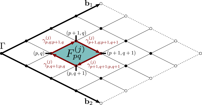
Figure 5: Discretization of the Brillouin zone spanned by reciprocal lattice vectors $\bm{b}_{1}$ and $\bm{b}_{2}$. Each vertex denoted by a black dot and labeled by indecies $(n,m)$ is associated to a plaquette. The Berry flux, $F^{(j)}_{nm}$, is calculated for each band on each plaquette. White dots depict vertices whose plaquettes are located in the adjacent Brillouin zone. (color online)

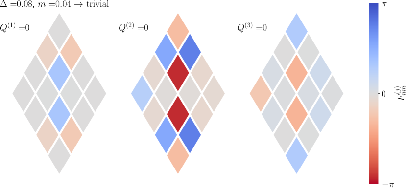
Figure 6: Calculated Chern numbers and the distribution of the Berry flux over the Brillouin zone in the absence of strain for the three occupied bands for topological and trivial phases.
(color online)

In this section we outline the calculation of the topological invariant of the investigated system. As the considered spin-orbit coupling preserves the $z$ component of the spin the $\mathbb{Z}_{2}$ invariant, characterizing time reversal invariant models, can be obtained from the parity of the total Chern number of the occupied band calculated for one of the spin species [21, 23].

Consider a discretization of the Brillouin zone depicted in Fig. 5. Assuming that the Brillouin is spanned by lattice vectors $\bm{b}_{1}$ and $\bm{b}_{2}$ we introduce sampling points labeled by $(p,q)$ corresponding to wavenumbers $\bm{k}=\frac{p\bm{b}_{1}}{N}+\frac{q\bm{b}_{2}}{N}$ with $N$ being a positive integer and $p,q\in[0,\dots,N-1]$. In Fig. 5 these points are depicted by black dots. For each vertex $(p,q)$ we denote the $j-$th eigenstate of the system by $|j;(p,q)\rangle$ For each vertex $(p,q)$ we associate a plaquette. Assuming that the spectrum of the system is non degenerate over the entire Brillouin zone the Chern number $Q^{(j)}$ for the $j-$th occupied band is the sum of Berry fluxes $F^{(j)}_{pq}$ for each plaquette

$$Q^{(j)}=\frac{1}{2\pi}\sum_{pq}F^{(j)}_{pq}.$$ (53)

The Berry fluxes $F^{(j)}_{pq}$ are in turn determined by the four phase angles

$$\gamma^{(j)}_{p,q;p^{\prime},q^{\prime}}=-\mathrm{arg}\left(\big{\langle}j;(p,q)\big{|}j;(p^{\prime},q^{\prime})\big{\rangle}\right),$$ (54)

defined on the edge bonds, denoted by red arrows in Fig. 5, corresponding to the given plaquette:

$$F_{pq}^{(j)}=-\text{arg}\left(\exp\left(-\text{i}\left[\gamma_{p,q;p+1,q}^{(j)}+\gamma_{p+1,q;p+1,q+1}^{(j)}\right.\right.\right.$$ (55)

$$\left.\left.\left.+\gamma_{p+1,q+1;p,q+1}^{(j)}+\gamma_{p,q+1;p,q}^{(j)}\right]\right)\right)$$

Assuming that the spectrum of the system is non degenerate the Chern number for a given band is obtained by the sum of the Berry fluxes for each plaquette in the Brillouin zone. The total Chern number $Q$ is the sum of the Chern numbers $Q^{(j)}$ of the occupied bands while the parity of $Q$ gives the topological invariant for the system investigated in the present manuscript. Even/odd Chern numbers correspond to a trivial/tropological phase.

As an illustration of the procedure we apply it to $H(\bm{k})$ defined in (42). First we note that the real periodicity of our model is dictated by the periodicity of the modulation characterized by the real space vectors $\bm{C}_{1}$ and $\bm{C}_{2}$ we shall denote the corresponding reciprocal lattice vectors by $\bm{b}^{C}_{1}$ and $\bm{b}^{C}_{2}$. In Fig. 6 we depict the calculated Berry fluxes and Chern numbers of the three lower bands, we considered as occupied, for a topological and for a trivial case. As one can observe already a modest $N=4$ discretization yields the right topological character for the investigated system.

References

• Awschalom and Samarth [2009] D. Awschalom and N. Samarth, Trend: Spintronics without magnetism, Physics 2, 50 (2009).
• Kuschel and Reiss [2015] T. Kuschel and G. Reiss, Spin orbitronics: Charges ride the spin wave, Nature nanotechnology 10, 22 (2015).
• Novoselov et al. [2004] K. S. Novoselov, A. K. Geim, S. V. Morozov, D. Jiang, Y. Zhang, S. V. Dubonos, I. V. Grigorieva, and A. A. Firsov, Electric field effect in atomically thin carbon films, Science 306, 666 (2004).
• Neto et al. [2009] A. C. Neto, F. Guinea, N. M. Peres, K. S. Novoselov, and A. K. Geim, The electronic properties of graphene, Reviews of modern physics 81, 109 (2009).
• Han et al. [2014] W. Han, R. K. Kawakami, M. Gmitra, and J. Fabian, Graphene spintronics, Nature nanotechnology 9, 794 (2014).
• Huertas-Hernando et al. [2009] D. Huertas-Hernando, F. Guinea, and A. Brataas, Spin-orbit-mediated spin relaxation in graphene, Physical review letters 103, 146801 (2009).
• Gamayun et al. [2018] O. Gamayun, V. Ostroukh, N. Gnezdilov, İ. Adagideli, and C. Beenakker, Valley-momentum locking in a graphene superlattice with Y-shaped Kekulé bond texture, New Journal of Physics 20, 023016 (2018).
• Hou et al. [2007] C.-Y. Hou, C. Chamon, and C. Mudry, Electron fractionalization in two-dimensional graphenelike structures, Physical Review Letters 98, 186809 (2007).
• Chamon [2000] C. Chamon, Solitons in carbon nanotubes, Physical Review B 62, 2806 (2000).
• Lin et al. [2017] Z. Lin, W. Qin, J. Zeng, W. Chen, P. Cui, J.-H. Cho, Z. Qiao, and Z. Zhang, Competing gap opening mechanisms of monolayer graphene and graphene nanoribbons on strong topological insulators, Nano Lett. 17, 4013 (2017), pMID: 28534404.
• Garza et al. [2014] H. H. P. Garza, E. W. Kievit, G. F. Schneider, and U. Staufer, Nano Letters 14, 4107 (2014).
• Jiang et al. [2017] Y. Jiang, J. Mao, J. Duan, X. Lai, K. Watanabe, T. Taniguchi, and E. Y. Andrei, Visualizing strain-induced pseudomagnetic fields in graphene through an hBN magnifying glass, Nano Letters 17, 2839 (2017).
• Guan and Du [2017] F. Guan and X. Du, Random gauge field scattering in monolayer graphene, Nano Letters 17, 7009 (2017).
• Goldsche et al. [2018] M. Goldsche, J. Sonntag, T. Khodkov, G. J. Verbiest, S. Reichardt, C. Neumann, T. Ouaj, N. von den Driesch, D. Buca, and C. Stampfer, Tailoring mechanically tunable strain fields in graphene, Nano Letters 18, 1707 (2018).
• Wang et al. [2019] L. Wang, S. Zihlmann, A. Baumgartner, J. Overbeck, K. Watanabe, T. Taniguchi, P. Makk, and C. Schönenberger, In situ strain tuning in hBN-encapsulated graphene electronic devices, Nano Letters 19, 4097 (2019).
• Wang et al. [2020] L. Wang, P. Makk, S. Zihlmann, A. Baumgartner, D. I. Indolese, K. Watanabe, T. Taniguchi, and C. Schönenberger, Mobility enhancement in graphene by in situ reduction of random strain fluctuations, Phys. Rev. Lett. 124, 157701 (2020).
• Andrade et al. [2019] E. Andrade, R. Carrillo-Bastos, and G. G. Naumis, Valley engineering by strain in Kekulé-distorted graphene, Physical Review B 99, 035411 (2019).
• Tajkov et al. [2019a] Z. Tajkov, D. Visontai, L. Oroszlány, and J. Koltai, Uniaxial strain induced topological phase transition in bismuth-tellurohalide–graphene heterostructures, Nanoscale 11, 12704 (2019a).
• Tajkov et al. [2019b] Z. Tajkov, D. Visontai, L. Oroszlány, and J. Koltai, Topological phase diagram of bitex–graphene hybrid structures, Applied Sciences 9, 4330 (2019b).
• Kane and Mele [2005] C. L. Kane and E. J. Mele, Quantum spin hall effect in graphene, Phys. Rev. Lett. 95, 226801 (2005).
• Fukui et al. [2005] T. Fukui, Y. Hatsugai, and H. Suzuki, Chern numbers in discretized brillouin zone: Efficient method of computing (spin) hall conductances, Journal of the Physical Society of Japan 74, 1674 (2005).
• Fukui and Hatsugai [2007] T. Fukui and Y. Hatsugai, Quantum spin hall effect in three dimensional materials: Lattice computation of z2 topological invariants and its application to bi and sb, Journal of the Physical Society of Japan 76, 053702 (2007).
• Asbóth et al. [2016] J. K. Asbóth, L. Oroszlány, and A. Pályi, A Short Course on Topological Insulators: Band Structure and Edge States in One and Two Dimensions, 1st ed., Lecture Notes in Physics, Vol. 909 (Springer International Publishing, BerlinXXX, 2016).
• Cooper et al. [2012] D. R. Cooper, B. D’Anjou, N. Ghattamaneni, B. Harack, M. Hilke, A. Horth, N. Majlis, M. Massicotte, L. Vandsburger, E. Whiteway, and V. Yu, Experimental Review of Graphene, ISRN Condens. Matter Phys. 2012, 1 (2012).
• Suzuura and Ando [2002] H. Suzuura and T. Ando, Phonons and electron-phonon scattering in carbon nanotubes, Phys. Rev. B 65, 235412 (2002).
• Mañes [2007] J. L. Mañes, Symmetry-based approach to electron-phonon interactions in graphene, Phys. Rev. B 76, 045430 (2007).
• Guinea et al. [2010] F. Guinea, M. Katsnelson, and A. Geim, Energy gaps and a zero-field quantum hall effect in graphene by strain engineering, Nature Physics 6, 30 (2010).
• Masir et al. [2013] M. R. Masir, D. Moldovan, and F. Peeters, Pseudo magnetic field in strained graphene: Revisited, Solid State Communications 175, 76 (2013).
• Naumis et al. [2017] G. G. Naumis, S. Barraza-Lopez, M. Oliva-Leyva, and H. Terrones, Electronic and optical properties of strained graphene and other strained 2d materials: a review, Reports on Progress in Physics 80, 096501 (2017).
• Reich et al. [2000] S. Reich, H. Jantoljak, and C. Thomsen, Shear strain in carbon nanotubes under hydrostatic pressure, Physical Review B 61, R13389 (2000).
• Gilvarry [1956] J. Gilvarry, Grüneisen parameter for a solid under finite strain, Physical Review 102, 331 (1956).
• Botello-Mendez et al. [2018] A. R. Botello-Mendez, J. C. Obeso-Jureidini, and G. G. Naumis, Toward an accurate tight-binding model of graphenes electronic properties under strain, The Journal of Physical Chemistry C 122, 15753 (2018).
• Faccio et al. [2009] R. Faccio, P. A. Denis, H. Pardo, C. Goyenola, and A. W. Mombrú, Mechanical properties of graphene nanoribbons, Journal of Physics: Condensed Matter 21, 285304 (2009).
• Scarpa et al. [2009] F. Scarpa, S. Adhikari, and A. S. Phani, Effective elastic mechanical properties of single layer graphene sheets, Nanotechnology 20, 065709 (2009).
• Turchi et al. [1998] P. E. Turchi, A. Gonis, and L. Colombo, Tight-Binding Approach to Computational Materials Science, Symposium Held December 1-3, 1997, Boston, Massachusetts, USA. Volume 491, Tech. Rep. (MATERIALS RESEARCH SOCIETY WARRENDALE PA, 1998).
• Pereira et al. [2009] V. M. Pereira, A. C. Neto, and N. Peres, Tight-binding approach to uniaxial strain in graphene, Physical Review B 80, 045401 (2009).
• Bena and Montambaux [2009] C. Bena and G. Montambaux, Remarks on the tight-binding model of graphene, New Journal of Physics 11, 095003 (2009).
• Spiegel and O’Donnell [1997] E. Spiegel and C. O’Donnell, Incidence algebras, Vol. 206 (CRC Press, 1997).
• Sólyom [2010] J. Sólyom, Fundamentals of the Physics of Solids: Volume 3-Normal, Broken-Symmetry, and Correlated Systems, Vol. 3 (Springer Science & Business Media, 2010).
• González-Árraga et al. [2018] L. González-Árraga, F. Guinea, and P. San-Jose, Modulation of kekulé adatom ordering due to strain in graphene, Phys. Rev. B 97, 165430 (2018).
• Oliva-Leyva and Naumis [2013] M. Oliva-Leyva and G. G. Naumis, Understanding electron behavior in strained graphene as a reciprocal space distortion, Physical Review B 88, 085430 (2013).
• Vozmediano et al. [2010] M. A. Vozmediano, M. Katsnelson, and F. Guinea, Gauge fields in graphene, Physics Reports 496, 109 (2010).