Toward accurate measurement of property-dependent galaxy clustering

Abstract

Galaxy clustering provides insightful clues to our understanding of galaxy formation and evolution, as well as the universe. The redshift assignment for the random sample is one of the key steps to measure the galaxy clustering accurately. In this paper, by virtue of the mock galaxy catalogs, we investigate the effect of two redshift assignment methods on the measurement of galaxy two-point correlation functions (hereafter 2PCFs), the ${V_{\rm max}}$ method and the “shuffled” method. We found that the shuffled method significantly underestimates both of the projected 2PCFs and the two-dimensional 2PCFs in redshift space. While the ${V_{\rm max}}$ method does not show any notable bias on the 2PCFs for volume-limited samples. For flux-limited samples, the bias produced by the ${V_{\rm max}}$ method is less than half of the shuffled method on large scales. Therefore, we strongly recommend the ${V_{\rm max}}$ method to assign redshifts to random samples in the future galaxy clustering analysis.

1 Introduction

Observed galaxy distribution encodes a wealth of information on the formation and evolution of galaxies, dark matter halos, and the large-scale structure of the universe. In the past two decades, with the successes of completed and ongoing wide-field surveys such as the Two Degree Field Galaxy Redshift Survey (2dFGRS; Colless et al. 2003), the Sloan Digital Sky Survey (SDSS; York et al. 2000), the Baryon Oscillation Spectroscopic Survey (BOSS; Eisenstein et al. 2011), the VIMOS Public Extragalactic Redshift Survey (VIPERS; Garilli et al. 2012), and the Dark Energy Spectroscopic Instrument (DESI; Levi et al. 2013; DESI Collaboration et al. 2016a, b), we are able to map the three-dimensional distribution of over a million galaxies with well-measured spectroscopic redshifts. These observed galaxies exhibit a variety of physical properties (e.g., luminosity, color, stellar mass, morphology, spectral type) as well as notable environment-dependent features (Dressler et al. 1997; Blanton et al. 2003a; Goto et al. 2003). Consequently one primary goal of observational cosmology is to utilize an efficient and reliable technique to optimally extract information from these samples, in order to interpret these property-dependent distributions and gain some cosmological insights.

The galaxy two-point correlation function is one of the most powerful and fundamental tools to characterize the spatial distribution of galaxies (Peebles 1980). On small scales, apart from the galaxy peculiar velocities (Jackson 1972; Hawkins et al. 2003; de la Torre et al. 2013), the 2PCF is shaped by the complex baryonic physics involved in galaxy formation in dark matter halos, offering unique checks for empirical galaxy-halo connection models, e.g., the halo occupation distribution model (HOD; Jing et al. 1998, 2002; Peacock & Smith 2000; Berlind & Weinberg 2002; Zheng et al. 2005; Guo et al. 2015; Xu et al. 2018), the conditional luminosity function technique (CLF; Yang et al. 2003, 2004, 2005a, 2005b, 2008, 2012, 2018; Vale & Ostriker 2004; van den Bosch et al. 2007), and the subhalo abundance matching method (SHAM;Kravtsov et al. 2004; Conroy et al. 2006; Vale & Ostriker 2006; Guo et al. 2010; Simha et al. 2012; Guo & White 2014; Chaves-Montero et al. 2016). On large scales, the anisotropy imprinted in the redshift-space clustering, arising from the gravity-driven coherent motion of matter, is widely used to measure the growth rate of the cosmic structure, to distinguish dark energy models and to constrain the cosmological parameters (Kaiser 1987; Peacock et al. 2001; Tegmark et al. 2004a; Seljak et al. 2006; Guzzo et al. 2008; Percival et al. 2010; Blake et al. 2011; Reid et al. 2012; Weinberg et al. 2013; Ross et al. 2014; Li et al. 2016; Shi et al. 2018; Wang et al. 2018). Therefore, to accurately measure the 2PCF is a critical step for probing the galaxy formation and cosmology.

To measure the galaxy 2PCF, we usually need a random sample with the same sky coverage and radial selection function as the galaxy sample (Hamilton 1993). For most redshift surveys, the observed galaxies are flux-limited samples suffering from luminosity-dependent selection bias. As the redshift increases, only luminous galaxies can be observed and the dim galaxies are too faint to be detected. As a result, the galaxy number density varies as a function of redshift. Generally, it is easy to produce random samples for the luminosity-selected galaxies if the luminosity function is fairly determined. However, for a galaxy sample selected by other physical quantities such as color, stellar mass, morphology and so forth, it is not straightforward to generate their corresponding random samples.

For these property-selected galaxy samples, the shuffled method has been widely used in galaxy clustering analysis (Li et al. 2006; Reid et al. 2012; Anderson et al. 2012; Sánchez et al. 2012; Guo et al. 2013; Ross et al. 2014). Previous tests have shown that the 2PCF measured using random sample constructed from the shuffled method produces the least biased result compared with other methods (Kazin et al. 2010; Howlett et al. 2015). Particularly, Ross et al. (2012) proved that the systematic bias induced by the shuffled method is quite small for the redshift-space correlation function on the scale around $30\sim 150{h^{-1}\rm Mpc}$, with a statistical uncertainty of at most $5\%$. However, as current and future redshift surveys are aiming at $\sim 1\%$ level accuracy of clustering measurements, the systematic bias induced by the shuffled method should be carefully taken into account. Generally, in the shuffled method, there is a hidden issue that the structures in the radial distribution of real galaxies can be transferred to the random sample through the shuffling process, resulting in an underestimation of galaxy clustering. By applying different approaches to construct the random samples, de la Torre et al. (2013) found that the projected 2PCF (hereafter P2PCF) measured using a random sample from the ${V_{\rm max}}$ method is more accurate than the measure from the shuffled method. This is not surprising since the random redshifts generated from the ${V_{\rm max}}$ method are randomly distributed in the maximum observable volume of the galaxies, only depending on the flux limits of the survey (Cole 2011). Therefore, in principle, the ${V_{\rm max}}$ method is superior to the shuffled method.

The purpose of this paper is to demonstrate that apart from the P2PCF, the shuffled method can impact the shape of the 2PCF in a 2D space, thus result in systematic errors in the redshift-space distortion measurement. While such kind of systematics is not induced in the ${V_{\rm max}}$ method. Here we use mock galaxy catalogs to quantify and compare the systematic uncertainty induced by random samples from the ${V_{\rm max}}$ method and the shuffled method. We primarily focus our tests on the galaxy clustering on scales below $40{h^{-1}\rm Mpc}$. For the ${V_{\rm max}}$ method, we also need to correctly estimate the maximum observable volume for individual galaxies based on the magnitude limits of the survey.

The paper is organized as follows. In Section 2, we first introduce how we construct the mock galaxy catalogs and prepare for our tests. Three radial distribution functions that we applied to produce the random samples are also outlined in this section. In Section 3, we compare the galaxy correlation functions measured from three different methods in detail and quantify the systematic uncertainties of these measurements. Finally, we discuss our results and conclude the paper in Section 4. In our distance calculation, we assume a flat $\Lambda$CDM cosmology with $\Omega_{m}=1-\Omega_{\Lambda}=0.268$, $h=H_{0}/(100\,{\rm km}\,\mathrm{s}^{-1}\mathrm{Mpc}^{-1})=0.71$.

2 Data

2.1 Construction of mocks

The mock galaxy catalogs are constructed basically in the same way as Yang et al. (2019). Briefly, we use a cosmological $N$-body simulation from the CosmicGrowth simulation suite (Jing 2019) named $\rm WMAP\_3072\_600$. This simulation was performed by executing a parallel adaptive $\rm P^{3}M$ code with $3072^{3}$ particles in a $600{h^{-1}\rm Mpc}$ cube box, assuming a standard flat $\Lambda\rm CDM$ cosmology with $\{\Omega_{m}=0.268,~{}\Omega_{b}=0.045,~{}\sigma_{8}=0.83,~{}n_{s}=0.968\}$ and $h=H_{0}/(100\,{\rm km}\,\mathrm{s}^{-1}\mathrm{Mpc}^{-1})=0.71$, which are consistent with the observation of the Nine-Year Wilkinson Microwave Anisotropy Probe (WMAP 9) (Bennett et al. 2013; Hinshaw et al. 2013). For each output snapshot, the friends-of-friends algorithm (Davis et al. 1985) is applied to find halos with a linking length of 0.2 in units of the mean particle separation. Then, the Hierarchical Bound-Tracing technique (Han et al. 2012, 2018) was used to identify subhalos along with their merger history. We pick the snapshot at $z=0$ to construct our halo catalog and halos containing at least 50 particles are included.

There are many popular galaxy-halo connection models that can successfully reproduce the observed galaxy clustering on different scales. Here, we apply the SHAM model to build the mock galaxy catalogs by assuming a monotonic relation between the galaxy absolute magnitude $M^{0.1}_{\rm r}$ and the peak mass $M_{\rm peak}$ of subhalos. The $M_{\rm peak}$ is defined as the maximum mass that a subhalo ever had throughout its evolutionary history. The luminosity function of SDSS DR7 ${\tt full\_1}$ sample of the New York University Value-Added catalog (NYU-VAGC) (Blanton et al. 2001, 2003b, 2005b) is adopted to perform the SHAM, where the $r-$band absolute magnitude $M^{0.1}_{\rm r}$ of galaxies have been $k-$ and $e-$corrected to redshift $z=0.1$. The ‘orphan’ galaxies are also taken into account in the halo catalog, see Yang et al. (2019) for details. A galaxy naturally obtains the position and velocity of a subhalo when it matches to the subhalo. By stacking the simulation box periodically and randomly setting the locations of the observers, we construct 60 mock galaxy catalogs in total. Galaxies in these mocks are complete at $M^{0.1}_{\rm r}\leq-18$, and their number density $n(z)$ should be the input $n_{\rm DR7}(z)$ but with a scatter due to cosmic variance. All mock galaxy catalogs have the same sky coverage of $\sim 2777\rm deg^{2}$ and the same radial comoving distance $d_{\rm C}$ of [0, 600] ${h^{-1}\rm Mpc}$. The true redshifts of galaxies are converted into the observed redshift $z_{\rm obs}$ by adding the influence of peculiar velocity. The apparent magnitude $m_{\rm r}$ is simply derived by $m_{\rm r}=M^{0.1}_{\rm r}+5\mathrm{log}_{10}[d_{\rm C}(1+z_{\rm obs})]+25$. In this study, as our vital goal is to identify the systematic bias in clustering measurements caused by different types of random samples, we use relatively simple models in constructing our mock galaxy catalogs to eliminate potential uncertainties. First, we do not add a scatter in the $M^{0.1}_{\rm r}-M_{\rm peak}$ matching relation, so that the galaxies selected in each realization corresponding to the same mass subhalos. Second, we ignore the $k-$ and $e-$corrections in all magnitude-related calculations. These simplifications will allow us to focus on testing the impact of random samples.

2.2 Mock galaxy catalog

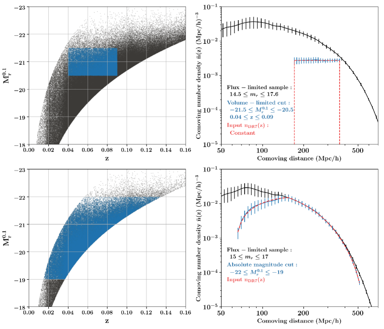
Figure 1: Galaxy distribution in redshift and $r$-band absolute magnitude for the mock galaxy catalog with different selection criteria (left panels), and comparison of the comoving number densities for these samples (right panels). In the upper-left panel, the gray points denote one of our flux-limited samples with apparent magnitude cuts $14.5\leq m_{\rm r}\leq 17.6$. We construct a volume-limited sample from this flux-limited sample as shown in the blue points, that we select galaxies within an absolute magnitude of [$-20.5$, $-21.5$] and a redshift range of [$0.04$, $0.09$]. The black curve in the upper-right panel is the mean comoving number density $\bar{n}(z)$ as a function of comoving distance for the 60 flux-limited mock samples. The error bars denote $1\sigma$ variation among these samples. The $\bar{n}(z)$ of the volume-limited samples are shown in the blue curve with error bars, which is constant as expected. The red dashed line represents the input $n_{\rm DR7}(z)$ of SDSS DR7 ${\tt full\_1}$ sample. For a flux-limited sample with $15\leq m_{\rm r}\leq 17$ as shown in the lower-left panel (in gray), we further make absolute magnitude cuts at $-22$ and $-19$ (in blue). The mean number density of different flux-limited samples is shown in the lower-right panel. Note, we use $h=H_{0}/(100\,{\rm km}\,\mathrm{s}^{-1}\mathrm{Mpc}^{-1})=0.71$ in our calculations (see text for details).

Galaxies observed in redshift surveys are usually flux-limited whose number density may vary as a function of redshift. In order to obtain a well-understood sample of galaxies for the measurement and modeling of the two-point statistics, a volume-limited sample or a magnitude cut flux-limited sample is usually constructed, at a cost of discarding a significant number of galaxies, therefore, lower the statistical accuracy (Zehavi et al. 2005; Xu et al. 2016). In this work, we construct both types of galaxy samples to carry out our tests.

Firstly, to define a volume-limited sample, we draw a flux-limited sample with apparent magnitude $14.5\leq m_{\rm r}\leq 17.6$ from each mock sample. Then, we specify an absolute magnitude range $-21.5\leq M^{0.1}_{\rm r}\leq-20.5$ and a redshift range $0.04\leq z_{\rm obs}\leq 0.09$ to the flux-limited sample, ensuring that a galaxy in the volume-limited sample can be displaced to any redshift in [0.04, 0.09] and still remains within the apparent magnitude limits (Norberg et al. 2001, 2002; Tegmark et al. 2004b; Zehavi et al. 2011). These constraints result in a constant comoving number density $n_{\rm const}$, and so is the radial selection function, hence, it is straightforward to create a random sample having exactly the same $n_{\rm const}$ as a volume-limited galaxy sample.

After that, we construct a set of magnitude cut flux-limited samples with apparent magnitude limits of $15\leq m_{\rm r}\leq 17$ and absolute magnitude $-22\leq M^{0.1}_{\rm r}\leq-19$ from the mocks. For a magnitude cut flux-limited sample, the galaxy number density is a strong function of redshift $n(z)$, as at a given redshift galaxies only in a certain absolute magnitude range can be detected by survey (Zehavi et al. 2002). The derivation of galaxy radial selection function needs to integrate the luminosity function of galaxy sample appropriately. In our case, we derive the expected comoving number density as a function of redshift for our flux-limited samples by equation:

$$n(z)=\int^{M^{0.1}_{\rm r,faint}(z)}_{M^{0.1}_{\rm r,bright}(z)}\Phi(M^{0.1}_{\rm r})dM^{0.1}_{\rm r},$$ (1)

where $\Phi(M^{0.1}_{\rm r})$ is the input luminosity function of the SDSS DR7 ${\tt full\_1}$ sample, and

$$M^{0.1}_{\rm r,bright}(z)=\mathtt{max}[M^{0.1}_{\rm r,min},15-DM(z)],$$ (2)

$$M^{0.1}_{\rm r,faint}(z)=\mathtt{min}[M^{0.1}_{\rm r,max},17-DM(z)],$$ (3)

where $DM(z)$ is the distance modulus at redshift $z$, and we set $M^{0.1}_{\rm r,min}=-22$ and $M^{0.1}_{\rm r,max}=-19$, respectively. The radial selection function $\phi(z)$ of the flux-limited sample can be estimated via equation:

$$\phi(z)=\frac{n(z)}{\int^{-19}_{-22}\Phi(M^{0.1}_{\rm r})dM^{0.1}_{\rm r}}.$$ (4)

As an example, we show a volume-limited sample and a flux-limited sample and the mean number densities of mock galaxy catalogs in Figure 1. In the upper-left panel, the blue points denote the galaxy distribution of the volume-limited sample on the redshift and absolute magnitude diagram, the raw flux-limited sample is denoted by the gray points. In the upper-right panel, the black and blue curves represent the mean number densities $\bar{n}(z)$ for the 60 flux-limited samples and volume-limited samples, respectively. The error bars stand for $1\sigma$ variation among these samples. The red dashed line marks the number density $n_{\rm DR7}(z)$ derived from the input luminosity function of SDSS DR7 ${\tt full\_1}$ sample. As expected, the $\bar{n}(z)$ of volume-limited samples agree very well with the constant $n_{\rm DR7}(z)$. The distributions of flux-limited samples are displayed in the lower panels of Figure 1. The mean $\bar{n}(z)$ of the flux-limited sample is a strong function of redshift, which again agrees with the $n_{\rm DR7}(z)$ estimated from equation (1) very well. Once the mean comoving number density is well estimated, we can easily construct the radial distribution of random samples for individual galaxy samples.

2.3 Random sample

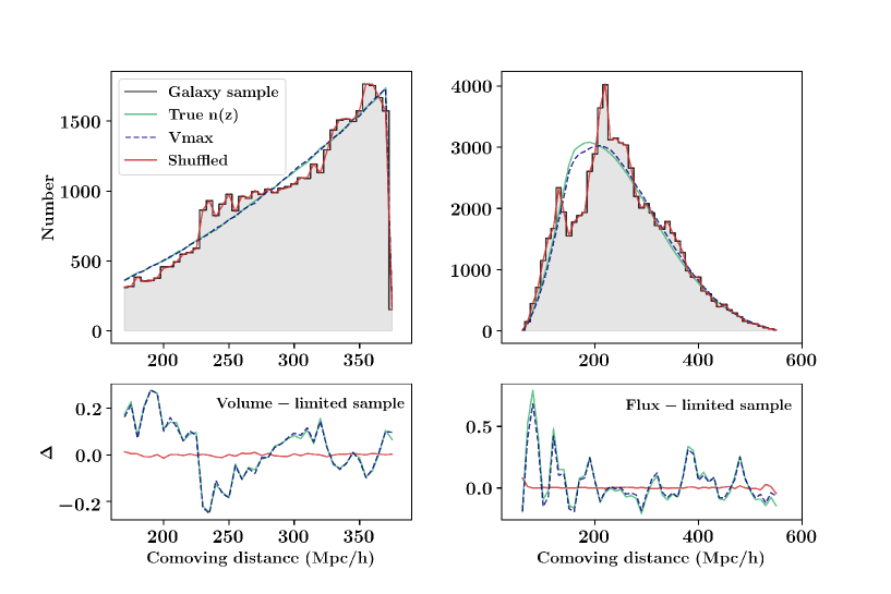
Figure 2: Comparison of radial distributions for galaxy sample and random samples. The shaded black histograms denote the distributions of a volume-limited sample (left panel) and a flux-limited sample (right panel) selected from our 60 mock galaxy samples. The bin sizes are $\Delta d=5{h^{-1}\rm Mpc}$ for the volume-limited sample and $\Delta d=10{h^{-1}\rm Mpc}$ for the flux-limited sample, respectively. The green, dashed blue and red curves represent the distributions of random samples generated by using the radial selection function derived from the true $n(z)$, the ${V_{\rm max}}$ method, and the shuffled method, separately. The total number of each random sample is scaled to be the same number as the galaxy sample. The lower small panels show the relative number bias in each distance of random points and galaxies, which is defined as $\Delta\equiv(n_{\rm r}-n_{\rm g})/n_{\rm g}$. $\Delta$ for different methods are coded in the same colors as the upper panels.

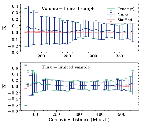
Figure 3: Mean of bias $\overline{\Delta}$ for 60 volume-limited samples (upper panel) and 60 flux-limited samples (lower panel), respectively. The green, blue and red curves denote the $\overline{\Delta}$ for the true $n(z)$, the ${V_{\rm max}}$ method, and the shuffled method, separately. Error bars stand for $1\sigma$ deviation of biases among these samples.

In this study, our basic goal is to identify the systematic uncertainty in galaxy clustering caused by random samples. More specifically, we aim to make a robust comparison of the ${V_{\rm max}}$ method and the shuffled method. The comparison will help us assess to what extent the random samples can impact our measurements of the 2PCFs.

Basically, we construct random samples for individual galaxy samples based on their radial distributions from three methods. First, we create a set of random points that uniformly distribute on the surface of a sphere, then points covering an equal area as the galaxy sample is selected. Without adding any angular selection effect, we take these points as the angular positions of the random samples. Theoretically, modeling the radial distribution of galaxy sample requires the true number density of galaxy sample. This is difficult to achieve in observation since we always sample galaxies in a certain volume of the universe, and the $n(z)$ can only be estimated empirically from the observed galaxies. By using mocks, the true number density $n(z)$ is the input $n_{\rm DR7}(z)$ as described in Section 2.2, therefore, allowing us to construct the $n(z)$ for random samples exactly identical to the true one. Three methods that are used to construct the radial distribution are described below:

1. True $n(z)$, where we apply the radial selection function $\phi(z)$ derived from equation (1) with the input $n_{\rm DR7}(z)$ to build the redshifts. In the following tests, we will use the correlation functions measured using the true $n(z)$ as the benchmarks and explore impacts of the ${V_{\rm max}}$ method or the shuffled method.

2. V_max method, where we uniformly spread random points in the maximum observable volume ${V_{\rm max}}$ of individual galaxies to obtain the radial comoving distance for random samples. For a volume-limited sample, ${V_{\rm max}}$ is a fixed volume at redshift range [0.04, 0.09]. For a flux-limited sample, we assign the absolute magnitudes of observed galaxies to random points, and their maximum/minimum redshifts $z_{\rm max,min}$ are estimated by

   $$z_{\rm max}=\mathtt{min}[z_{\rm m,max},z_{\rm sample,max}],$$ (5)

   $$z_{\rm min}=\mathtt{max}[z_{\rm m,min},z_{\rm sample,min}].$$ (6)

   and

   $$m_{\rm r,faint}=M^{0.1}_{\rm r,faint}+DM(z_{\rm m,max}),$$ (7)

   $$m_{\rm r,bright}=M^{0.1}_{\rm r,bright}+DM(z_{\rm m,min}).$$ (8)

   where we set $m_{\rm r,bright}=15$, $m_{\rm r,faint}=17$, $M^{0.1}_{\rm r,bright}=-22$, and $M^{0.1}_{\rm r,faint}=-19$ based on the magnitude cuts to the flux-limited samples.

3. Shuffled method, where we randomly select redshifts from the galaxy samples and assign the redshifts to the corresponding random samples.

As an example, Figure 2 demonstrates the distribution of radial comoving distance for the two types of galaxy samples (shaded black histograms) in one of our realizations, as well as the random samples generated using the radial selection function $\phi(z)$ estimated from the true $n(z)$ (green curves), the ${V_{\rm max}}$ method (blue dashed curves), and the shuffled method (red curves), respectively. The bin size is $\Delta d=5{h^{-1}\rm Mpc}$ for the volume-limited sample and $\Delta d=10{h^{-1}\rm Mpc}$ for the flux-limited sample. We also compute the number difference $\Delta$ of random samples relative to the galaxy samples as shown in the lower small panels. We define the difference as $\Delta\equiv(n_{\rm r}-n_{\rm g})/n_{\rm g}$, where $n_{\rm r}$ and $n_{\rm g}$ denote the number of random points and galaxies in each distance bin. The mean difference $\overline{\Delta}$ of individual $\Delta$ for all 60 realizations are displayed in Figure 3. The error bars represent the standard deviation from $\overline{\Delta}$ among all samples in each bin. Apparently, random samples constructed using the shuffled method show the best agreement with the radial distribution of galaxies for both the volume-limited samples and the flux-limited samples, indicating the structures of galaxies in the line-of-sight direction are reserved. Radial distributions constructed by the true $n(z)$ and the ${V_{\rm max}}$ method are nearly identical, especially for the volume-limited samples. Meanwhile, the two distributions exhibit small deviations from each other in the flux-limited sample. As mentioned before, this is due to the fact that each observation is actually one sampling of a small set of galaxies in the universe. The larger the observed galaxy sample, the closer the number density is to the true $n(z)$. Moreover, we see that the distribution given by the ${V_{\rm max}}$ method seems slightly closer to the distribution of the galaxy sample. This difference indicates that the ${V_{\rm max}}$ method still suffers very slightly from the large-scale structure as noted by Blanton et al. (2005a), which may impact the luminosity function and hence the redshift distribution of our random points.

3 Clustering measurement

In this section, we will compare galaxy correlation functions measured using three different random samples, to demonstrate that using the one constructed from the shuffled method leads to an underestimation of galaxy clustering. While the measurements using the ${V_{\rm max}}$ random sample has much better performance on all scales that we explored.

3.1 Clustering estimator

We use the common way to calculate the correlation function (Huchra 1988; Hamilton 1992; Fisher et al. 1994) in a 2D space, that the redshift separation vector $\mathbf{s}$ and the line-of-sight vector $\mathbf{l}$ are defined as $\mathbf{s}\equiv\mathbf{v}_{1}-\mathbf{v}_{2}$ and $\mathbf{l}\equiv(\mathbf{v}_{1}+\mathbf{v}_{2})/2$, separately, where $\mathbf{v}_{1}$ and $\mathbf{v}_{2}$ are the redshift space position vectors of a pair of galaxies. The separations parallel ($\pi$) and perpendicular ($r_{p}$) to the line of sight are derived as

$$\pi\equiv\frac{\mathbf{s}\cdot\mathbf{l}}{|\mathbf{l}|},~{}~{}~{}~{}~{}~{}r^{2}_{p}\equiv\mathbf{s}\cdot\mathbf{s}-\pi^{2}.$$ (9)

A grid of $\pi$ and $r_{p}$ is constructed by taking $1{h^{-1}\rm Mpc}$ as the bin size for $\pi$ from 0 linearly up to $\pi_{\rm max}=60{h^{-1}\rm Mpc}$ and $0.2$ dex as the bin size for $r_{p}$ logarithmically in the range of [$0.01$, $60$] ${h^{-1}\rm Mpc}$. The estimator of Landy & Szalay (1993) is adopted as

$$\xi(r_{p},\pi)=\frac{DD-2DR+RR}{RR},$$ (10)

where $DD$, $DR$, and $RR$ are the numbers of data-data, data-random, and random-random pairs. Then, by integrating the $\xi(r_{p},\pi)$ along the line-of-sight separation we estimate the P2PCF (Davis & Peebles 1983) by

$$w_{p}(r_{p})\equiv 2\int^{\infty}_{0}\xi(r_{p},\pi)~{}d\pi=2\int^{\pi_{max}}_{0}\xi(r_{p},\pi)~{}d\pi.$$ (11)

In this work, we run $\tt{CORRFUNC}$ (Sinha & Garrison 2019) for pair counting to measure all mock galaxy correlation functions. In order to reduce the shot noise, we use random samples which are $\sim$ 40 times the number of galaxies.

3.2 Comparison of correlation functions

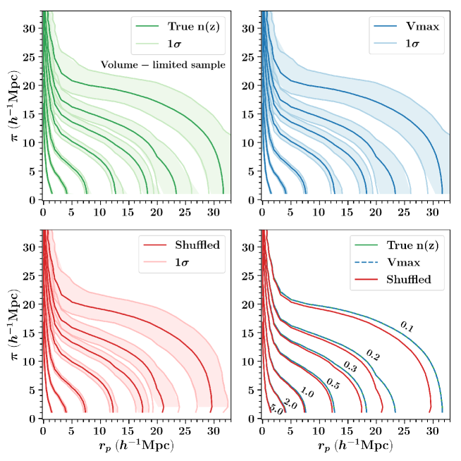
Figure 4: The average correlation function contours $\overline{\xi}(r_{p},\pi)$ measured using random samples constructed with the true $n(z)$ (top-left panel), the ${V_{\rm max}}$ method (top-right panel), and the shuffled method (bottom-left panel) for the volume-limited samples, respectively. The shaded regions mark $1\sigma$ deviations among 60 mock samples. The bottom-right figure shows comparison of $\overline{\xi}(r_{p},\pi)$ for different methods. The contour levels from outside-in correspond to $\overline{\xi}(r_{p},\pi)=[0.1,0.2,0.3,0.5,1,2,5]$, respectively.

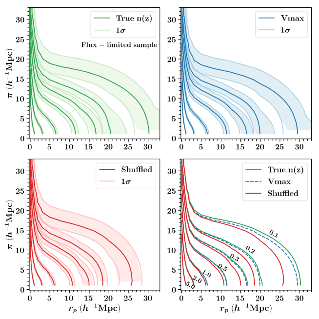
Figure 5: The same as Figure 4 but for the flux-limited samples.

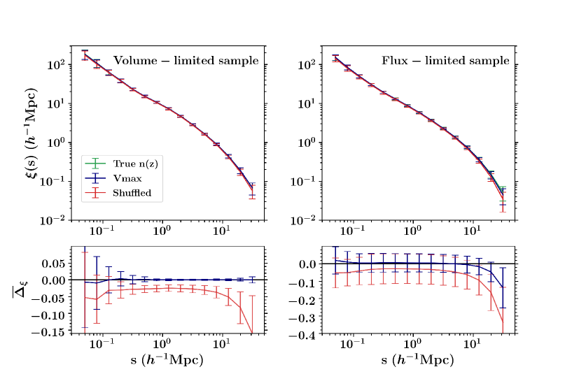
Figure 6: Top panels: The average redshift-space correlation functions $\xi(s)$ of 60 volume-limited samples (left) and 60 flux-limited samples (right) and their standard deviations (error bars). The green curves represent the true $\xi(s)$ measured using random samples from the true $n(z)$, the blue and red curves denote the $\xi(s)$ for the ${V_{\rm max}}$ method and the shuffled method, respectively. Bottom panels: The average bias $\overline{\Delta}_{\xi}$ and $1\sigma$ deviations from the true $\xi(s)$ for the two radial selection models, determined using 60 mock galaxy catalogs.

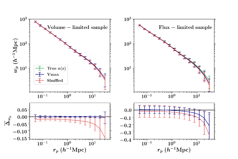
Figure 7: The same as Figure 6 but for the projected two-point correlation functions.

Our main results in comparison of the 2PCFs measured from three different methods are presented in this section. We consider the correlation function measured from the true $n(z)$ as the true 2PCF. The comparison of the correlation function contours, the redshift-space correlation functions, and the projected two-point correlation functions are shown in Figure 4 to Figure 7, respectively.

Figure 4 and Figure 5 display the average contours of the two-dimensional correlation functions $\xi(r_{p},\pi)$ for the volume-limited samples and the flux-limited samples, respectively. The true $\xi(r_{p},\pi)$ (hereafter $\xi_{\rm true}(r_{p},\pi)$) derived from the true $n(z)$ is denoted by the green contours in the top-left panel, the shaded light green regions represent $1\sigma$ variance among 60 individual measurements of $\xi_{\rm true}(r_{p},\pi)$. The blue and red contours in the top-right panel and the bottom-left panel denote the $\xi(r_{p},\pi)$ of the ${V_{\rm max}}$ method and the shuffled method (hereafter $\xi_{\rm Vmax}(r_{p},\pi)$ and $\xi_{\rm shuffled}(r_{p},\pi)$) , separately. Comparison of the average $\xi(r_{p},\pi)$ for all three different methods is shown in the bottom-right panel, where $\xi_{\rm Vmax}$ is denoted by the dashed blue contours to distinguish from $\xi_{\rm true}$. For the volume-limited samples, the $\xi_{\rm Vmax}(r_{p},\pi)$ contours are generally indistinguishable from the $\xi_{\rm true}(r_{p},\pi)$ contours. For the flux-limited samples, $\xi_{\rm Vmax}(r_{p},\pi)$ contours exhibit overall great agreement with the true ones, with a very small systematic bias at large radii well below the $1\sigma$ uncertainty.

For the case of shuffled method, the $\xi_{\rm shuffled}(r_{p},\pi)$ exhibit a prominent systematic bias from $\xi_{\rm true}(r_{p},\pi)$ for both types of samples, especially for the flux-limited samples where the bias is almost beyond $1\sigma$ statistical uncertainty. Note that since the systematic bias indeed changes the shape of $\xi(r_{p},\pi)$, which will induce systematic errors in the cosmological probes using the redshift distortion effects on intermediate scales (see e.g. Shi et al. 2018).

The comparison of the average redshift-space correlation functions $\xi(s)$ is shown in the upper panels of Figure 6. The left panel displays the mean $\overline{\Delta}_{\xi}$ of 60 volumed-limited mock samples, the right panel shows the same results but for the flux-limited samples. The true $\xi_{\rm true}(s)$ is denoted by the green curve. The $\xi(s)$ from the ${V_{\rm max}}$ method and the shuffled method are in blue and red curves, respectively. The error bars represent $1\sigma$ variance among $\xi(s)$. The lower panels show the mean bias $\overline{\Delta}_{\xi}$ of $\xi_{\rm Vmax}(s)$ and $\xi_{\rm shuffled}(s)$ with respect to $\xi_{\rm true}(s)$. The mean bias is defined as $\overline{\Delta}_{\xi}=(\sum^{N}_{i=1}\Delta^{i}_{\xi})/N$, where $\Delta^{i}_{\xi}=(\xi^{i}_{\rm Vmax}-\xi^{i}_{\rm true})/\xi^{i}_{\rm true}$ for ${V_{\rm max}}$ method or $\Delta^{i}_{\xi}=(\xi^{i}_{\rm shuffled}-\xi^{i}_{\rm true})/\xi^{i}_{\rm true}$ for shuffled method, the $\xi^{i}$ is the correlation function of the $i$th galaxy sample, and $N=60$. The error bars denote $1\sigma$ variance of 60 individual $\Delta^{i}_{\xi}$. We can clearly see that, the comparison results are completely consistent with the results shown in Figure 4 and Figure 5. For the volume-limited samples, the mean bias of $\xi_{\rm Vmax}$ relative to $\xi_{\rm true}$ is almost zero. Comparatively, there is a systematic bias of $\sim 3\%$ between $\xi_{\rm shuffled}$ and $\xi_{\rm true}$ at small scales. On scales above $8{h^{-1}\rm Mpc}$, the bias gradually increases. At the scale of $\sim 30{h^{-1}\rm Mpc}$, the mean bias $\overline{\Delta}_{\xi,\rm shuffled}$ is up $\sim 15\%$. For the flux-limited samples, the ${V_{\rm max}}$ method also exhibits much better performance than the shuffled method. On scale below $10{h^{-1}\rm Mpc}$, $\xi_{\rm Vmax}$ is fairly identical to $\xi_{\rm true}$, and $\xi_{\rm shuffled}$ exhibits an underestimate with a bias up to $\sim 5\%$. On scales $s>10{h^{-1}\rm Mpc}$, both methods display underestimates to a certain extent, where the $\overline{\Delta}_{\xi,\rm Vmax}$ gradually increases to $12\%$ at the scale of $30{h^{-1}\rm Mpc}$ and the $\overline{\Delta}_{\xi,\rm shuffled}$ is $\sim 30\%$ on the same scale.

Finally, comparison of the average P2PCFs are shown in Figure 7, where the color-coded $w_{p}$ from three different methods are the same as Figure 6. We can see that, without the effect of redshift distortion, $w_{p,\rm Vmax}$ remains roughly identical to $w_{p,\rm true}$ for the volume-limited samples (left panels), and for the flux-limited samples (right panels) $w_{p,\rm Vmax}$ also agrees with $w_{p,\rm true}$ on scale smaller than $1{h^{-1}\rm Mpc}$. While, on larger scale, the ${V_{\rm max}}$ method results in a slightly increasing underestimation compared with the true one, and $\overline{\Delta}_{w_{p,\rm Vmax}}$ is also kind of larger than $\overline{\Delta}_{\xi,\rm Vmax}$. As for the shuffled method, on scale of $r_{p}<1{h^{-1}\rm Mpc}$, the average $w_{p,\rm shuffled}$ shows less deviation from $w_{p,\rm true}$ compared with the results of redshift-space correlation functions for both types of samples. The mean deviation of $w_{p,\rm shuffled}$ from $w_{p,\rm true}$ increases with a strong bias above scales of $1{h^{-1}\rm Mpc}$. The $\overline{\Delta}_{w_{p,\rm shuffled}}$ is up to $15\%$ for the volume-limited samples and $34\%$ for the flux-limited samples at $30{h^{-1}\rm Mpc}$, respectively.

Based on the above comparison, our results steadily demonstrate that using random samples constructed from the ${V_{\rm max}}$ method to measure the correlation function, we can achieve much higher accuracy than those from the shuffled method. For the volume-limited samples, the average correlation functions from the ${V_{\rm max}}$ method are almost identical to the true correlation functions on all concerned scales, with nearly zero bias and negligible statistical uncertainty. For the flux-limited samples, on scales smaller than $10{h^{-1}\rm Mpc}$ for $\xi(s)$ and $1{h^{-1}\rm Mpc}$ for $w_{p}(r_{p})$, the average correlation functions from the ${V_{\rm max}}$ method are still fully consistent with the true correlation functions with a statistical uncertainty of at most $5\%$. As the scale increases, the correlation functions from the ${V_{\rm max}}$ method tends to underestimate the galaxy clustering slightly. Nevertheless, the mean bias from the ${V_{\rm max}}$ method is still much smaller than the bias from the shuffled method in general.

4 Discussion ans conclusion

In this paper, using mock galaxy catalogs, we have investigated the systematic bias induced by random samples generated using the ${V_{\rm max}}$ method and the shuffled method in galaxy clustering measurement. We have compared the redshift-space correlation functions and the projected 2PCFs for the volume-limited samples and the flux-limited samples, respectively. Our results demonstrate that the ${V_{\rm max}}$ method is more robust to simulate the radial distribution of galaxies for the random sample. Our main results can be summarized as follows:

1. For the volume-limited samples, the ${V_{\rm max}}$ method can produce an unbiased measure of galaxy clustering on the scale less than $40{h^{-1}\rm Mpc}$, while, the shuffled method results in an increasing systematic underestimation with the increase of scale.

2. For the flux-limited samples, the 2PCFs measured from random samples of the ${V_{\rm max}}$ method remain unbiased concerning the true galaxy clustering on small scales. While on scales larger than $10{h^{-1}\rm Mpc}$, both methods display a systematic bias beyond the systematic uncertainty, but the ${V_{\rm max}}$ method still has better performance than the shuffled method.

3. By comparing the correlation contours, we find that the shuffled method can significantly underestimate the squashing effect on large scales, which may induce potential systematics in cosmological probes using the linear redshift distortion effect.

4. Finally, the projected 2PCF measured from the shuffled method still produces an underestimation, especially on scales larger than $2{h^{-1}\rm Mpc}$. This scale is also known as the “two-halo term” scale (Mo & White 1996; Sheth & Tormen 1999; Cooray & Sheth 2002). Thus, if galaxy clustering measured from the redshift shuffled random samples are used as constraints, a non-negligible systematic bias will be introduced to models such as the halo model, galaxy formation models, and the galaxy-halo connection models.

Based on the above tests, we suggest using the ${V_{\rm max}}$ method to generate random samples. The galaxy correlation function from the ${V_{\rm max}}$ method can recover the galaxy clustering more accurately, then providing more reliable and stringent constraints on the models of galaxy formation and cosmology.

Besides, there are some simplifications in our probes to be noted as well. In this paper, we ignored the $k-$ and $e-$ corrections in our tests, however, these corrections need to be carefully handled when the analysis is performed to the observed galaxies. To determine these corrections, one should fit the spectral templates to the galaxy spectrum or the broad-band photometry (Blanton & Roweis 2007), and the fitting results largely depend on the assumptions of the galaxy star formation history, the stellar population synthesis model, and the dust extinction model (Kroupa 2001; Pforr et al. 2012). While, as long as the maximum observable volume of individual galaxies is estimated correctly, our conclusions still firmly hold. In addition, we also note that the systematic bias from the shuffled method determined by Ross et al. (2012) is somewhat smaller than ours for the redshift-space correlation function at scale $\sim 30{h^{-1}\rm Mpc}$. One possible reason is that our tests performed with the low redshift galaxies of SDSS DR7, with a median redshift at $\sim 0.1$. But the BOSS CMASS data that they studied is a high-redshift sample with a median redshift at $\sim 0.52$, where they have a larger volume. All in all, we are confident in our tests, that the ${V_{\rm max}}$ method is a more robust way to measure the galaxy clustering. We will adopt this method to investigate the property-dependent galaxy clustering in our future works.