22institutetext: School of Astronomy and Space Science,University of Chinese Academy of Sciences, Beijing 100049, China 33institutetext: Centre for High Energy Physics, Peking University, Beijing 100871, China
Cosmological constraints on ultra-light axion fields
Abstract
Ultra-light axions (ULAs) with mass less than eV have interesting behaviors that may contribute to either dark energy or dark matter at different epochs of the Universe. Its properties can be explored by cosmological observations, such as expansion history of the Universe, cosmic large-scale structure, cosmic microwave background, etc. In this work, we study the ULAs with a mass around eV, that means the ULA field still rolls slowly at present with the equation of state as dark energy. In order to investigate the mass and other properties of this kind of ULA field, we adopt the measurements of Type Ia supernova (SN Ia), baryon acoustic oscillation (BAO), and Hubble parameter . The Markov Chain Monte Carlo (MCMC) technique is employed to perform the constraints on the parameters. Finally, by exploring four cases of the model, we find that the mass of this ULA field is about eV if assuming the initial axion field . We also investigate a general case by assuming , and find that the fitting results of are consistent with or close to 1 for the datasets we use.
keywords:
Cosmology: Dark energy : Cosmological parameters1 Introduction
Axion or axion-like particle (ALP) is a good candidate for cold dark matter (CDM) (Peccei & Quinn 1977; Weinberg 1978; Wilczek 1978). It was proposed to solve the strong CP problem in the Quantum Chromodynamics (QCD) theory, and generated by breaking the Peccei-Quinn (PQ) symmetry (Peccei & Quinn 1977). Axion has a huge possible mass range spanning over many orders of magnitude, that cannot be stringently constrained by theory. In the string theory, axion is allowed to have extremely small mass, i.e. ultra-light axion (ULA), which ranges from to eV or even smaller (Witten 1984; Svrcek & Witten 2006; Marsh 2016). Some interesting properties of ULAs appear in this mass range.
In the early Universe, the Hubble parameter is larger than axion mass , i.e. (the natural units are used with hereafter). Then the axion field is overdamped by the Hubble friction and would roll slowly. It means the ULA equation of state acting as dark energy with negative pressure. Later, when the Universe expanding slowly and slowly, we have . At this time, the ULA field is underdamped and begins to oscillate. The equation of state of ULA also oscillates correspondingly between -1 and 1, which has an average value acting as dark matter. Since the mass of ULAs is quite small, the de Broglie wavelength of ULAs can be large enough to affect the formation of cosmic structure at galaxy or sub-galaxy scales, which is similar to the free-streaming effect of warm dark matter. Therefore, the ULAs can contribute to both dark energy and dark matter at different epochs of the Universe.
For , the ULAs begin to oscillate before the epoch of the radiation-matter equality ( eV), and since then behave like dark matter with energy density , that can contribute to all of dark matter in this mass range(Iršič et al. 2017; Armengaud et al. 2017; Bar et al. 2019; Marsh & Niemeyer 2019; Nebrin et al. 2019). On the other hand, for eV, the ULAs will oscillate after the radiation-matter equality, and can contribute to the late accelerating expansion of the Universe as dark energy (Marsh & Ferreira 2010; Hlozek et al. 2015; Marsh 2016).
In this work, we explore the ULAs with mass , which means where eV is the present Hubble constant. It implies that the axion field has not or just entered the oscillation stage and still acts as dark energy at present with the equation of state around -1. The data of Type Ia supernova (SN Ia), baryon acoustic oscillation (BAO), and Hubble parameters at different redshifts are used to constrain this kind of ULA filed and its mass. The Markov Chain Monte Carlo (MCMC) method is adopted in the constraint to derive the probability distribution functions (PDFs) of the parameters in the model.
The paper is organized as follows: in Section 2, we discuss the ultra-light axion model and derive the relevant equations used in the constraint; in Section 3, we describe the SN Ia, BAO, and H(z) data we adopt in the fitting process; in Section 4, we show the constraint result; we summarize and discuss the result in Section 5.
2 Model
The action of the ultra-light axion field is given by
| (1) |
where is the canonically normalized axion field which has a shift symmetry , and is a periodic potential with the minimum at . A simple choice of is given by (Marsh & Ferreira 2010; Hlozek et al. 2015; Marsh 2016).
| (2) |
Here is the amplitude of the potential which indicates the energy scale of non-perturbative physics, and is the PQ symmetry-breaking energy scale. Expanding the potential for as a Taylor series, then the dominant term is
| (3) |
where the axion mass is given by . We can find that the axion mass can be extremely small if , which is the case we discuss in this work.
Assuming a flat Friedmann-Robertson-Walker (FRW) metric, the variation of the action with given in Eq. (3), the equation of motion can be derived as
| (4) |
Here is the Hubble parameter, and is the scale factor. The energy density and pressure of the axion field can be also obtained from the energy momentum tensor as
| (5) | |||||
| (6) |
In the radiation or matter dominated era, we have where or , respectively. In this case, Eq. (4) has an exact solution, and it is found that for at early time (), and begins to oscillate for at late time (), where is the scale factor when oscillation occurs (Hlozek et al. 2015; Marsh 2016). Then the equation of state of the axion field can be derived from Eq. (5) and (6). For extremely small (or ), and , and we can find that , which means the axion filed behaves like dark energy (DE, e.g. cosmological constant) with constant energy density. On the other hand, for large (or ), will oscillate around 0 between -1 and 1, that acts like ordinary matter.
For DE-like axion field, the energy density parameter , where , and is the current critical density, where is the Hubble constant in and is the Planck mass. Considering is quite small that the ultra-light axion field has not begun to oscillate at present (i.e. ), and then we have
| (7) |
where is the initial homogeneous axion field, and (Hlozek et al. 2015; Marsh 2016). We will explore the constraints for and cases, respectively, in the following discussion. Then, in our model, the Hubble parameter can be written as
| (8) | |||||
| (9) |
Here , is the matter energy density parameter, and is the cosmic curvature parameter. The comoving distance can be estimated by
| (10) |
where , , and for open, flat, and closed geometries, respectively.
3 Data
3.1 SN Ia data
We adopt Pantheon SN Ia sample in the constraints, which contains 1048 SNe Ia from Pan-STARRS1 (PS1), Sloan Digital Sky Survey (SDSS), SNLS, and various low-z and Hubble Space Telescope samples in the range (Scolnic et al. 2018). The distribution is used to estimate the likelihood function , and it can be written as
| (11) |
Here where and are the vectors of observational and theoretical apparent magnitudes, respectively, and is the covariance matrix. where is the theoretical distance modulus, and is the absolute magnitude. It can be further expressed as
| (12) | |||||
| (13) |
Here is the luminosity distance, is the Hubble-constant free luminosity distance, and is a nuisance parameter that is combined with the Hubble constant and . The covariance matrix takes the form as
| (14) |
where is the vector of statistic error, which includes photometric error of the SN distance, uncertainties of distance from the mass step correction, the distance bias correction, the peculiar velocity, redshift measurement, stochastic gravitational lensing, and the intrinsic scatter. is the systematic covariance matrix for the data (Scolnic et al. 2018).
3.2 BAO data
| Redshift | Measurement | Value | Survey | References | |
|---|---|---|---|---|---|
| 0.106 | 0.33600.015 | – | 6dFGS | (Beutler et al. 2011) | |
| 0.15 | 0.22390.0084 | – | SDSS DR7 | (Ross et al. 2015) | |
| 0.32 | 0.11810.0024 | – | BOSS LOW-Z | (Anderson et al. 2014) | |
| 0.57 | 0.07260.0007 | – | BOSS CMASS | (Padmanabhan et al. 2012) | |
| 0.44 | 0.08700.0042 | – | WiggleZ | (Blake et al. 2012) | |
| 0.60 | 0.06720.0031 | – | WiggleZ | (Blake et al. 2012) | |
| 0.73 | 0.05930.0020 | – | WiggleZ | (Blake et al. 2012) | |
| 2.34 | 0.03200.0013 | – | SDSS-III DR11 | (Delubac et al. 2015) | |
| 2.36 | 0.03290.0009 | – | SDSS-III DR11 | (Hell et al. 2015) | |
| 0.15 | 66425 | 148.69 | SDSS DR7 | (Aubourg et al. 2015) | |
| 1.52 | 3843147 | 147.78 | SDSS DR14 | (Ata et al. 2018) | |
| 0.38 | 151822 | 147.78 | SDSS DR12 | (Alam et al. 2017) | |
| 0.51 | 197727 | 147.78 | SDSS DR12 | (Alam et al. 2017) | |
| 0.61 | 228332 | 147.78 | SDSS DR12 | (Alam et al. 2017) | |
| 2.40 | 36.61.2 | – | SDSS DR12 | (du Mas des Bourboux et al. 2017) | |
| 2.40 | 8.940.22 | – | SDSS DR12 | (du Mas des Bourboux et al. 2017) |
In Table 1, we list the adopted quantities that derived from the BAO surveys. is the radius of the comoving sound horizon at the drag epoch, which takes the form as
| (15) |
where is the sound speed, is the epoch of last scattering, is the scale factor. Since are not sensitive to physics at low redshifts, we find that it will not be affected in our model significantly. Hence, for simplicity, we fix the value as given by Planck 2018 result (Planck Collaboration et al. 2018). The spherically averaged distance is given by
| (16) |
where is the comoving angular diameter distance, and is the physical angular diameter distance. is the Hubble distance.
The for the BAO data can be estimated by
| (17) |
where , and and are the observational and theoretical quantities shown in Table 1. is the corresponding covariance matrix.
3.3 data
The data are also used in this work, which contains 51 data points in the redshift ranging from 0 to 2.36 (see Table 1 in Geng et al. 2018). These data are measured by the two methods. The first method is called the differential-age method, that is proposed to compare the ages of passively-evolving galaxies with similar metallicity, as cosmic chronometers, separated in a small redshift interval (Jimenez & Loeb 2002) The second one is using the BAO measurement as a standard ruler along the radial direction (Gaztañaga et al. 2009).
The of the data is given by
| (18) |
Here and are the observational and theoretical Hubble parameters, respectively, and is the error.
Finally, the joint of the three datasets is given by
| (19) |
By fitting these three datasets, we will constrain the mass of DE-like ULA filed and other parameters assuming and , respectively, in the flat and non-flat Universe.
4 Constraint Results
In order to constrain the free parameters, the MCMC technique is adopted in this work. We make use of the public code 111https://baudren.github.io/montepython.html to perform the constraint, and the Metropolis-Hastings algorithm is employed to extract the chain points. Four cases in our model are explored, i.e. in flat and non-flat spaces, and in flat and non-flat spaces. The flat priors are taken for the free parameters, and set as follow: , , , , and the SN Ia absolute magnitude . In each case, we generate 20 chains and totally obtain 1,000,000 chain points to illustrate the 1-D and 2-D probability distribution functions (PDFs) of the free parameters.
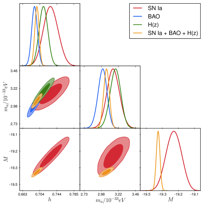
| Parameter | SN Ia | BAO | SN Ia+BAO+ | |
| eV | ||||
| 0.982 | 1.624 | 1.104 | 0.997 |
In Figure 1, we show the contour maps and 1-D PDFs of , , and for and flat case. The best-fits and 1- errors of the parameters for the SN Ia, BAO, , and joint datasets have been shown in Table 2, respectively. The reduced chi-square is also shown, where is the minimum , and and are the numbers of data and free parameters, respectively. We find that our model can fit the data well, since for the SN Ia, , and SN Ia+BAO+ data, and for the BAO data. The best-fits of are around 0.7 for the BAO, , and SN Ia+BAO+ datasets from 0.69 to 0.71, and the result from SN Ia only is a bit high that . The results of are basically consistent in 1- for the four datasets giving eV. The nuisance parameter, the absolute magnitude shown in Eq. (12), in the SN Ia data is also considered in the fitting process, and the results from SN Ia only and SN Ia+BAO+ are in a good agreement.
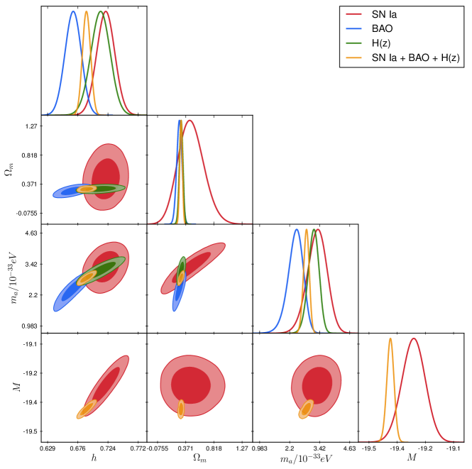
| Parameter | SN Ia | BAO | SN Ia+BAO+ | |
| eV | ||||
| 1.072 | 1.612 | 1.129 | 0.997 |
The fitting results of , , , and for and non-flat case are shown in Figure 2 and Table 3. We find that the fitting is as good as the flat case, but the constraint results from SN Ia data is significantly looser than other datasets, which is due to the combination effect of non-flat assumption and additional parameter . We also notice that, although the best-fit of from SN Ia only is as large as , it is consistent with the results from other dataset in 1- with the best-fitting . The SN Ia dataset gives obviously larger and compared to BAO dataset in this case, but basically the four datasets provide similar results as the flat case, that and eV.
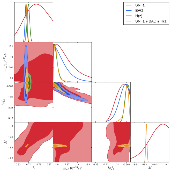
| Parameter | SN Ia | BAO | SN Ia+BAO+ | |
| eV | ||||
| 1.011 | 1.382 | 1.002 | 0.976 |
In Figure 3 and Table 4, we show the constraint results of , , , and for and flat case. We find that the constraints on the parameters are generally looser than the case, especially for the SN Ia data (with additional nuisance parameter ), since there are strong degeneracies between and both and as shown in Eq. (7). The SN Ia data cannot provide stringent constraint on , which gives the best-fitting with large error, but it is still consistent with the results from other datasets giving . The best-fits of are basically lower than the case, especially for the BAO data, that we have eV with the lower limits of 1- values close to zero for the four datasets. The best-fits of are around , and the upper limits of 1- are consistent with 0 (i.e. ) for the SN Ia, BAO, and datasets. This means is a good assumption in this model.
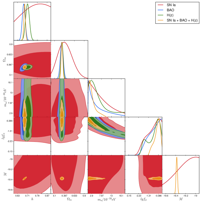
| Parameter | SN Ia | BAO | SN Ia+BAO+ | |
| eV | ||||
| 1.009 | 1.281 | 1.103 | 0.981 |
In Figure 4 and Table 5, we show the fitting results for and non-flat case. The constraint results are similar to the and flat case, but have larger uncertainties since one more parameter is included. Again, we find that the best-fits of are eV, and lower limits of 1- of are close to zero. Also, The upper limits of are consistent with (for SN Ia, BAO, and only) or close to 1 (joint dataset).
5 Summary
In this work, we study the ULA field with mass around eV that , which means the ULA field still rolls slowly or just starts to enter the oscillation stage and can be treated as dark energy so far. We make use of the data from SN Ia, BAO, and to constrain the properties of ULA field, and the MCMC technique is adopted to perform the data fitting process. The mass of the DE-like ULA field , the ratio of initial field to the Planck mass , the matter density parameter , reduced Hubble parameter , and the SN Ia absolute magnitude are considered in the fitting process.
Four cases of the model are explored in this work, assuming the initial ULA field and in flat and non-flat space, respectively. We find that the best-fits of are around eV assuming in either flat or non-flat space. When assuming , the constraints become significantly looser, and we find the best-fits of become smaller, and the lower limits of 1- are consistent with zero. Besides, the fitting results of are close to 0 for both flat and non-flat cases, which means the assumption of is a good choice in this model. Besides the observational data adopted in this work, other datasets can be used to further improve the constraint results, such as the cosmic microwave background, weak lensing, galaxy cluster, and so on. We will investigate these constraint results in our future work.
6 Acknownledgments
JGK and YG acknowledges the support of NSFC-11822305, NSFC-11773031, NSFC-11633004, the Chinese Academy of Sciences (CAS) Strategic Priority Research Program XDA15020200, the NSFC-ISF joint research program No. 11761141012, and CAS Interdisciplinary Innovation Team.
References
- Alam et al. (2017) Alam, S., Ata, M., Bailey, S., et al. 2017, MNRAS, 470, 2617
- Anderson et al. (2014) Anderson, L., Aubourg, É., Bailey, S., et al. 2014, MNRAS, 441, 24
- Armengaud et al. (2017) Armengaud, E., Palanque-Delabrouille, N., Yèche, C., Marsh, D. J. E., & Baur, J. 2017, MNRAS, 471, 4606
- Ata et al. (2018) Ata, M., Baumgarten, F., Bautista, J., et al. 2018, MNRAS, 473, 4773
- Aubourg et al. (2015) Aubourg, É., Bailey, S., Bautista, J. E., et al. 2015, Phys. Rev. D, 92, 123516
- Bar et al. (2019) Bar, N., Blum, K., Lacroix, T., & Panci, P. 2019, Journal of Cosmology and Astroparticle Physics, 2019, 045
- Beutler et al. (2011) Beutler, F., Blake, C., Colless, M., et al. 2011, MNRAS, 416, 3017
- Blake et al. (2012) Blake, C., Brough, S., Colless, M., et al. 2012, MNRAS, 425, 405
- Delubac et al. (2015) Delubac, T., Bautista, J. E., Busca, N. G., et al. 2015, A&A, 574, A59
- du Mas des Bourboux et al. (2017) du Mas des Bourboux, H., Le Goff, J.-M., Blomqvist, M., et al. 2017, A&A, 608, A130
- Gaztañaga et al. (2009) Gaztañaga, E., Cabré, A., & Hui, L. 2009, MNRAS, 399, 1663
- Geng et al. (2018) Geng, J.-J., Guo, R.-Y., Wang, A.-Z., Zhang, J.-F., & Zhang, X. 2018, Communications in Theoretical Physics, 70, 445
- Hell et al. (2015) Hell, S. W., Sahl, S. J., Bates, M., et al. 2015, Journal of Physics D Applied Physics, 48, 443001
- Hlozek et al. (2015) Hlozek, R., Grin, D., Marsh, D. J. E., & Ferreira, P. G. 2015, Phys. Rev. D, 91, 103512
- Iršič et al. (2017) Iršič, V., Viel, M., Haehnelt, M. G., Bolton, J. S., & Becker, G. D. 2017, Phys. Rev. Lett., 119, 031302
- Jimenez & Loeb (2002) Jimenez, R., & Loeb, A. 2002, ApJ, 573, 37
- Marsh (2016) Marsh, D. J. E. 2016, Phys. Rep., 643, 1
- Marsh & Ferreira (2010) Marsh, D. J. E., & Ferreira, P. G. 2010, Phys. Rev. D, 82, 103528
- Marsh & Niemeyer (2019) Marsh, D. J. E., & Niemeyer, J. C. 2019, Phys. Rev. Lett., 123, 051103
- Nebrin et al. (2019) Nebrin, O., Ghara, R., & Mellema, G. 2019, Journal of Cosmology and Astroparticle Physics, 2019, 051
- Padmanabhan et al. (2012) Padmanabhan, N., Xu, X., Eisenstein, D. J., et al. 2012, MNRAS, 427, 2132
- Peccei & Quinn (1977) Peccei, R. D., & Quinn, H. R. 1977, Phys. Rev. Lett., 38, 1440
- Planck Collaboration et al. (2018) Planck Collaboration, Aghanim, N., Akrami, Y., et al. 2018, arXiv:1807.06209
- Ross et al. (2015) Ross, A. J., Samushia, L., Howlett, C., et al. 2015, MNRAS, 449, 835
- Scolnic et al. (2018) Scolnic, D. M., Jones, D. O., Rest, A., et al. 2018, ApJ, 859, 101
- Svrcek & Witten (2006) Svrcek, P., & Witten, E. 2006, Journal of High Energy Physics, 2006, 051
- Weinberg (1978) Weinberg, S. 1978, Phys. Rev. Lett., 40, 223
- Wilczek (1978) Wilczek, F. 1978, Phys. Rev. Lett., 40, 279
- Witten (1984) Witten, E. 1984, Communications in Mathematical Physics, 92, 455