A convergent algorithm for forced mean curvature flow driven by diffusion on the surface

Abstract

The evolution of a closed two-dimensional surface driven by both mean curvature flow and a reaction–diffusion process on the surface is formulated as a system that couples the velocity law not only to the surface partial differential equation but also to the evolution equations for the normal vector and the mean curvature on the surface. Two algorithms are considered for the obtained system. Both methods combine surface finite elements for space discretization and linearly implicit backward difference formulae for time integration. Based on our recent results for mean curvature flow, one of the algorithms directly admits a convergence proof for its full discretization in the case of finite elements of polynomial degree at least two and backward difference formulae of orders two to five, with optimal-order error bounds. Numerical examples are provided to support and complement the theoretical convergence results (illustrating the convergence behaviour of both algorithms) and demonstrate the effectiveness of the methods in simulating a three-dimensional tumour growth model.

2010 Mathematics Subject Classification: Primary 35R01; 65M60; 65M15; 65M12.

Keywords: forced mean curvature flow; reaction–diffusion on surfaces; evolving finite element method; linearly implicit; backward difference formula; convergence; tumour growth.

1 Introduction

We consider the numerical approximation of an unknown evolving two-dimensional closed surface $\Gamma(t)$ that is driven by both mean curvature flow and a reaction–diffusion process on the surface, starting from a given smooth initial surface $\Gamma^{0}$. The outer normal velocity $V$ of the surface is determined by the velocity law

$$V=-H+u,$$ (1.1)

where $H$ is the mean curvature of the evolving surface, and where $u(x,t)$ ($x\in\Gamma(t)$, $t\in[0,T]$) is the solution of a reaction–diffusion equation on the evolving surface,

$$\partial^{\bullet}u+u\,\nabla_{\Gamma}\cdot v-\varDelta_{\Gamma}u=F(u,\nabla_{\Gamma}u),$$ (1.2)

with given initial data $u^{0}$. Here, $F:\mathbb{R}\times\mathbb{R}^{3}\rightarrow\mathbb{R}$ is a given smooth function, and $v$ is the surface velocity: $v=V\nu$ with $V$ of (1.1) and the outer normal $\nu$. Problem (1.1)–(1.2) can be viewed as forced mean curvature flow driven by the solution of the parabolic equation (1.2) on the evolving surface.

While we study the numerical approximation of Problem (1.1)–(1.2) with a scalar parabolic equation for notational simplicity, we remark that the numerical method and its convergence properties extend readily to the case of a system of reaction-diffusion equations (1.2) with solution $u=(u_{1},\dots,u_{m})$ and the velocity law $V=-H+\alpha_{1}u_{1}+\ldots+\alpha_{m}u_{m}$ with constant real coefficients $\alpha_{i}$. We will encounter such a more general problem in our numerical experiments with a tumour growth model.

Many practical applications concern mean curvature flow coupled with surface partial differential equations (PDEs), for example tumour growth [8, 9, 7, 2, 23]; surface dissolution [22, 18] (also see [16, Section 10.4]); diffusion induced grain boundary motion [24, 11, 36]. These models all use a velocity law that is linear in $u$, as in (1.1) or as in the previous paragraph, except for diffusion induced grain boundary motion where $V=-H+u^{2}$.

Numerical approximations to forced mean curvature flow coupled with surface partial differential equations have been considered in some of these papers. For curves, convergence of numerical methods for such coupled problems of forced curve shortening flow was proved in [35, 3].

Numerical approximation to pure mean curvature flow of surfaces — i.e. the case $u\equiv 0$ in (1.1) — was first addressed by Dziuk [14], based on a formulation of mean curvature flow as a formally heat-like equation on a surface. He proposed an evolving surface finite element method in which the moving nodes of the finite element mesh determine the approximate evolving surface. Different surface finite element based methods were proposed by Barrett, Garcke & Nürnberg [5] based on different variational formulations, and by Elliott & Fritz [20] based on DeTurck’s trick of reparametrizing the surface. However, proving convergence of any of these methods has remained an open problem for the mean curvature flow of closed two-dimensional surfaces.

In [28] we proved the first convergence result for semi- and full discretizations of mean curvature flow of closed surfaces with evolving surface finite elements. Discretizing the coupled system for the velocity law together with evolution equations for the normal vector field and mean curvature, we obtained a method with provable error bounds of optimal order.

To our knowledge, no convergence results have yet been proved for forced mean curvature flow of closed surfaces (1.1)–(1.2). For a regularized version of forced mean curvature flow of closed surfaces, optimal-order convergence results for semi- and full discretizations were obtained in [29] and [30], respectively.

In this paper, we extend the approach and techniques of our previous paper [28] to the forced mean curvature flow problem (1.1)–(1.2) as a coupled problem together with evolution equations for the normal vector and mean curvature. These evolution equations, as compared with those for pure mean curvature flow given in [26], contain additional forcing terms depending on $u$. We present two fully discrete evolving finite element algorithms for the obtained coupled system. The first algorithm discretizes the two terms $\partial^{\bullet}u+u\,\nabla_{\Gamma[X]}\cdot v$ separately in the spatial discretization by using the velocity law for $v$ and the approach in [28]. The second algorithm combines the two terms in the spatial discretization by an idea of [15] for treating conservation laws on an evolving surface. Both algorithms use evolving surface finite elements for spatial discretization and linearly implicit backward difference formulae for time integration, and for both algorithms the moving nodes of a finite element mesh determine the approximate evolving surface.

The convergence proof for the forced mean curvature algorithm considered here is a very minor modification compared to the convergence proof for the pure mean curvature algorithm of [28], since that algorithm is already built on coupling evolution equations on the surface to the evolution of the surface. The first algorithm can be written in the same matrix–vector form as the method proposed in [28] for the mean curvature flow. The convergence analysis in [28] applies directly to the present algorithm for forced mean curvature flow as well, except for one term which corresponds to the term $\Delta_{\Gamma}u$ in the evolution equation for $H$. The necessary changes to the stability analysis brought about by this term are carried out in detail. Under the assumption that the problem admits a sufficiently regular solution, this yields uniform in time, optimal-order $H^{1}$-norm convergence results for the semi- and full discretizations of forced mean curvature flow when using at least quadratic evolving surface FEM and linearly implicit backward difference formulae of order two to five.

For the second algorithm, we indicate how such an optimal-order convergence estimate of the evolving surface finite element semi-discretization can be obtained by combining results of [29] and [28], but we do not carry out the details.

For the velocity law $V=-H+g(u)$ with a nonlinear smooth function $g$, we expect that convergence of a direct generalization of the algorithms presented in this paper can be shown with a combination of the techniques of [28, 29, 32]. As this would become a nontrivial lengthy extension, it is not worked out here.

Finally, we present numerical experiments to support and complement the theoretical results. We present convergence tests for both algorithms, and also present an experiment with the numerical simulation for a tumour growth model, using the parameters in [2] for the sake of easy comparison.

2 Evolution equations for mean curvature flow driven by diffusion on the surface

2.1 Basic notions and notation

We consider the evolving two-dimensional closed surface $\Gamma(t)\subset\mathbb{R}^{3}$ for times $t\in[0,T]$ as the image

$$\Gamma(t)=\Gamma[X(\cdot,t)]:=\{X(p,t)\,:\,p\in\Gamma^{0}\},$$

of a smooth flow map $X:\Gamma^{0}\times[0,T]\rightarrow\mathbb{R}^{3}$ such that $X(\cdot,t)$ is an embedding for every $t$. Here, $\Gamma^{0}$ is a smooth closed initial surface, and $X(p,0)=p$. When the time $t$ is clear from the context, we drop $t$ in the notation and write for short

$$\Gamma[X]=\Gamma[X(\cdot,t)].$$

In view of the subsequent numerical discretization, it is convenient to think of $X(p,t)$ as the position at time $t$ of a moving particle with label $p$, and of $\Gamma[X]$ as a collection of such particles.

The velocity $v(x,t)\in\mathbb{R}^{3}$ at a point $x=X(p,t)\in\Gamma(t)$ equals

$$\partial_{t}X(p,t)=v(X(p,t),t).$$ (2.1)

For a known velocity field $v$, the position $X(p,t)$ at time $t$ of the particle with label $p$ is obtained by solving the ordinary differential equation (2.1) from $0$ to $t$ for a fixed $p$.

For a function $w(x,t)$ ($x\in\Gamma(t)$, $0\leq t\leq T$) we denote the material derivative as

$$\partial^{\bullet}w(x,t)=\frac{\text{d}}{\text{d}t}\,w(X(p,t),t)\quad\hbox{ for }\ x=X(p,t).$$

On any regular surface $\Gamma\subset\mathbb{R}^{3}$, we denote by $\nabla_{\Gamma}w:\Gamma\rightarrow\mathbb{R}^{3}$ the tangential gradient of a function $w:\Gamma\rightarrow\mathbb{R}$, and in the case of a vector field $f=(f_{1},f_{2},f_{3})^{T}:\Gamma\rightarrow\mathbb{R}^{3}$, we let $\nabla_{\Gamma}f=(\nabla_{\Gamma}f_{1},\nabla_{\Gamma}f_{2},\nabla_{\Gamma}f_{3})$. We thus use the convention that the gradient of $f$ has the gradient of the components as column vectors. We denote by $\nabla_{\Gamma}\cdot f$ the surface divergence of a vector field $f$ on $\Gamma$, and by $\varDelta_{\Gamma}w=\nabla_{\Gamma}\cdot\nabla_{\Gamma}w$ the Laplace–Beltrami operator applied to $w$; see the review [10] or [17, Appendix A] or any textbook on differential geometry for these notions.

We denote the unit outer normal vector field to $\Gamma$ by $\nu:\Gamma\rightarrow\mathbb{R}^{3}$. Its surface gradient contains the (extrinsic) curvature data of the surface $\Gamma$. At every $x\in\Gamma$, the matrix of the extended Weingarten map,

$$A(x)=\nabla_{\Gamma}\nu(x),$$

is a symmetric $3\times 3$ matrix (see, e.g., [37, Proposition 20]). Apart from the eigenvalue $0$ with eigenvector $\nu$, its other two eigenvalues are the principal curvatures $\kappa_{1}$ and $\kappa_{2}$. They determine the fundamental quantities

$$H:={\rm tr}(A)=\kappa_{1}+\kappa_{2},\qquad|A|^{2}=\kappa_{1}^{2}+\kappa_{2}^{2},$$ (2.2)

where $|A|$ denotes the Frobenius norm of the matrix $A$. Here, $H$ is called the mean curvature (as in most of the literature, we do not put a factor 1/2).

2.2 Evolution equations for normal vector and mean curvature

Forced mean curvature flow driven by diffusion on the surface sets the velocity (2.1) of the surface $\Gamma[X]$ to

$$v=V\nu\quad\ \text{ with the normal velocity }\quad V=-H+u,$$ (2.3)

where $u$ is the solution of the non-linear reaction–diffusion equation on the surface $\Gamma[X]$ with given initial value $u^{0}$,

$$\partial^{\bullet}u+u\nabla_{\Gamma[X]}\cdot v-\varDelta_{\Gamma[X]}u=F(u,\nabla_{\Gamma[X]}u)\quad\hbox{ on }\quad\Gamma[X],$$ (2.4)

with a given smooth function $F:\mathbb{R}\times\mathbb{R}^{3}\rightarrow\mathbb{R}$.

The geometric quantities $H$ and $\nu$ on the right-hand side of (2.3) satisfy the following evolution equations, which are modifications of the evolution equations for pure mean curvature flow (i.e., $V=-H$) as derived by Huisken [26].

Lemma 2.1.

For a regular surface $\Gamma[X]$ moving under forced mean curvature flow (2.3), the normal vector and the mean curvature satisfy

$$\partial^{\bullet}\nu =\varDelta_{\Gamma[X]}\nu+|A|^{2}\,\nu-\nabla_{\Gamma[X]}u,$$ (2.5)

$$\partial^{\bullet}H =\varDelta_{\Gamma[X]}H+|A|^{2}H-\varDelta_{\Gamma[X]}u-|A|^{2}u.$$ (2.6)

Proof.

Using the normal velocity $V$ in the proof of [26, Lemma 3.3], or see also [6, Lemma 2.37], the following evolution equation for the normal vector holds:

$$\partial^{\bullet}\nu=-\nabla_{\Gamma[X]}V.$$

On any surface $\Gamma$, it holds true that (see [17, (A.9)] or [37, Proposition 24])

$$\nabla_{\Gamma[X]}H=\varDelta_{\Gamma[X]}\nu+|A|^{2}\nu,$$

which, in combination with $V=-H+u$ from (2.3), gives the stated evolution equation for $\nu$.

By revising the proof of [26, Theorem 3.4 and Corollary 3.5], or see [6, Lemma 2.39], with the normal velocity $V$ we obtain

$$\partial^{\bullet}H=-\varDelta_{\Gamma[X]}V-|A|^{2}V,$$

which, again with $V=-H+u$ from (2.3), yields the evolution equation for $H$. ∎

2.3 The system of equations used for discretization

Similarly to [28], collecting the above equations, we have reformulated forced mean curvature flow as the system of semi-linear parabolic equations (2.5)–(2.6) on the surface coupled to the velocity law (2.3) and the surface PDE (2.4). The numerical discretization is based on a weak formulation of (2.3)–(2.6), together with the velocity equation (2.1). For the velocity law (2.3) we use a weak formulation that turns into the standard Ritz projection when restricted to a subspace. The weak formulation reads, with $V=-H+u$ and $A=\nabla_{\Gamma[X]}\nu$,

$$\int_{\Gamma[X]}\!\!\!\!\nabla_{\Gamma[X]}v\cdot\nabla_{\Gamma[X]}\varphi^{v}+\!\int_{\Gamma[X]}\!\!\!\!v\cdot\varphi^{v}=\!\int_{\Gamma[X]}\!\!\!\!\!\nabla_{\Gamma[X]}(V\nu)\cdot\nabla_{\Gamma[X]}\varphi^{v}+\int_{\Gamma[X]}\!\!\!\!\!V\nu\cdot\varphi^{v}$$ (2.7a)

$$\int_{\Gamma[X]}\!\!\!\!\partial^{\bullet}\nu\cdot\varphi^{\nu}+\int_{\Gamma[X]}\!\!\!\!\nabla_{\Gamma[X]}\nu\cdot\nabla_{\Gamma[X]}\varphi^{\nu}=\int_{\Gamma[X]}\!\!\!\!|A|^{2}\,\nu\,\cdot\varphi^{\nu}-\int_{\Gamma[X]}\!\!\!\!\nabla_{\Gamma[X]}u\cdot\varphi^{\nu}$$ (2.7b)

$$\int_{\Gamma[X]}\!\!\!\!\!\partial^{\bullet}H\,\varphi^{H}\!+\!\int_{\Gamma[X]}\!\!\!\!\!\nabla_{\Gamma[X]}H\cdot\nabla_{\Gamma[X]}\varphi^{H}=\!-\int_{\Gamma[X]}\!\!\!\!\!|A|^{2}\,V\,\varphi^{H}$$

$$\ \phantom{\int_{\Gamma[X]}\!\!\!\!\!\partial^{\bullet}H\,\varphi^{H}\!+\!\int_{\Gamma[X]}\!\!\!\!\!\nabla_{\Gamma[X]}H\cdot\nabla_{\Gamma[X]}\varphi^{H}=}+\!\int_{\Gamma[X]}\!\!\!\!\!\nabla_{\Gamma[X]}u\cdot\nabla_{\Gamma[X]}\varphi^{H},$$ (2.7c)

$$\frac{\text{d}}{\text{d}t}\int_{\Gamma[X]}u\varphi^{u}+\int_{\Gamma[X]}\nabla_{\Gamma[X]}u\cdot\nabla_{\Gamma[X]}\varphi^{u}=\int_{\Gamma[X]}F(u,\nabla_{\Gamma[X]}u)\varphi^{u},$$ (2.8)

for all test functions $\varphi^{v}\in H^{1}(\Gamma[X])^{3}$ and $\varphi^{\nu}\in H^{1}(\Gamma[X])^{3}$, $\varphi^{H}\in H^{1}(\Gamma[X])$, and $\varphi^{u}\in H^{1}(\Gamma[X])$ with $\partial^{\bullet}\varphi^{u}=0$. Here, we use the Sobolev space $H^{1}(\Gamma)=\{u\in L^{2}(\Gamma)\,:\,\nabla_{\Gamma}u\in L^{2}(\Gamma)\}$. Throughout the paper both the usual Euclidean scalar product for vectors and the Frobenius inner product for matrices (which equals to the Euclidean product using an arbitrary vectorization) are denoted by a dot. This system is complemented with the initial data $X^{0}$, $\nu^{0}$, $H^{0}$ and $u^{0}$.

An alternative weak formulation of (2.8), which is similar to (2.7b)–(2.7), is based on

$$\ \int_{\Gamma[X]}\partial^{\bullet}u\,\varphi^{u}+\int_{\Gamma[X]}\nabla_{\Gamma[X]}u\cdot\nabla_{\Gamma[X]}\varphi^{u}=\int_{\Gamma[X]}F(u,\nabla_{\Gamma[X]}u)\varphi^{u}-\int_{\Gamma[X]}\big{(}\nabla_{\Gamma[X]}\cdot v\big{)}u\varphi^{u},$$

for $\varphi^{u}\in H^{1}(\Gamma[X])$. Using that $\nabla_{\Gamma}V\cdot\nu=0$ and $H=\nabla_{\Gamma[X]}\cdot\nu$ and inserting the velocity law (2.3), we obtain

$$\nabla_{\Gamma[X]}\cdot v= \ \nabla_{\Gamma[X]}\cdot(V\nu)=(\nabla_{\Gamma[X]}V)\cdot\nu+V(\nabla_{\Gamma[X]}\cdot\nu)=V(\nabla_{\Gamma[X]}\cdot\nu)$$

$$= \ \color[rgb]{0,0,0}(-H+u)H.$$

This yields a weak formulation of a similar form as (2.7b) and (2.7),

$$\ \int_{\Gamma[X]}\partial^{\bullet}u\,\varphi^{u}+\int_{\Gamma[X]}\nabla_{\Gamma[X]}u\cdot\nabla_{\Gamma[X]}\varphi^{u}=\int_{\Gamma[X]}f(H,u,\nabla_{\Gamma[X]}u)\varphi^{u}$$ (2.9)

for all $\varphi^{u}\in H^{1}(\Gamma[X])$, where we set

$$f(H,u,\nabla_{\Gamma[X]}u)=F(u,\nabla_{\Gamma[X]}u)-(-H+u)Hu.$$

3 Evolving finite element semi-discretization

3.1 Evolving surface finite elements

We formulate the evolving surface finite element (ESFEM) discretization for the velocity law coupled with evolution equations on the evolving surface, following the description in [29, 28], which is based on [13] and [12]. We use a surface approximation consisting of curved elements of polynomial degree $k$ over a flat triangular reference element, which are therefore simply called triangles (even if they are curved), and use continuous piecewise polynomial basis functions of degree $k$, as defined in [12, Section 2.5].

We triangulate the given smooth initial surface $\Gamma^{0}$ by an admissible family of triangulations $\mathcal{T}_{h}$ of decreasing maximal element diameter $h$; see [15] for the notion of an admissible triangulation, which includes quasi-uniformity and shape regularity. For a momentarily fixed $h$, we denote by ${\mathbf{x}}^{0}$ the vector in $\mathbb{R}^{3N}$ that collects all nodes $p_{j}$ $(j=1,\dots,N)$ of the initial triangulation. By piecewise polynomial interpolation of degree $k$, the nodal vector defines an approximate surface $\Gamma_{h}^{0}$ that interpolates $\Gamma^{0}$ in the nodes $p_{j}$ of the (curved) triangles of $\mathcal{T}_{h}$. We will evolve the $j$th node in time according to an approximation of the ODE (2.1), denoted $x_{j}(t)$ with $x_{j}(0)=p_{j}$, and collect the nodes at time $t$ in a column vector

$${\mathbf{x}}(t)\in\mathbb{R}^{3N}.$$

We just write ${\mathbf{x}}$ for ${\mathbf{x}}(t)$ when the dependence on $t$ is not important.

By piecewise polynomial interpolation on the plane reference triangle that corresponds to every curved triangle of the triangulation, the nodal vector ${\mathbf{x}}$ defines a closed surface denoted by $\Gamma_{h}[{\mathbf{x}}]$. We can then define globally continuous finite element basis functions

$$\phi_{i}[{\mathbf{x}}]:\Gamma_{h}[{\mathbf{x}}]\rightarrow\mathbb{R},\qquad i=1,\dotsc,N,$$

which have the property that on every triangle their pullback to the reference triangle is polynomial of degree $k$, and which satisfy at the nodes $\phi_{i}[{\mathbf{x}}](x_{j})=\delta_{ij}$ for all $i,j=1,\dotsc,N.$ These functions span the finite element space on $\Gamma_{h}[{\mathbf{x}}]$,

$$S_{h}[{\mathbf{x}}]=S_{h}(\Gamma_{h}[{\mathbf{x}}])=\textnormal{span}\big{\{}\phi_{1}[{\mathbf{x}}],\phi_{2}[{\mathbf{x}}],\dotsc,\phi_{N}[{\mathbf{x}}]\big{\}}.$$

For a finite element function $u_{h}\in S_{h}[{\mathbf{x}}]$, the tangential gradient $\nabla_{\Gamma_{h}[{\mathbf{x}}]}u_{h}$ is defined piecewise on each element.

The discrete surface at time $t$ is parametrized by the initial discrete surface via the map $X_{h}(\cdot,t):\Gamma_{h}^{0}\rightarrow\Gamma_{h}[{\mathbf{x}}(t)]$ defined by

$$X_{h}(p_{h},t)=\sum_{j=1}^{N}x_{j}(t)\,\phi_{j}[{\mathbf{x}}(0)](p_{h}),\qquad p_{h}\in\Gamma_{h}^{0},$$

which has the properties that $X_{h}(p_{j},t)=x_{j}(t)$ for $j=1,\dots,N$, that $X_{h}(p_{h},0)=p_{h}$ for all $p_{h}\in\Gamma_{h}^{0}$, and

$$\Gamma_{h}[{\mathbf{x}}(t)]=\Gamma[X_{h}(\cdot,t)]=\{X_{h}(p_{h},t)\,:\,p_{h}\in\Gamma_{h}^{0}\}.$$

The discrete velocity $v_{h}(x,t)\in\mathbb{R}^{3}$ at a point $x=X_{h}(p_{h},t)\in\Gamma[X_{h}(\cdot,t)]$ is given by

$$\partial_{t}X_{h}(p_{h},t)=v_{h}(X_{h}(p_{h},t),t).$$

In view of the transport property of the basis functions [15], $\tfrac{\text{d}}{\text{d}t}\big{(}\phi_{j}[{\mathbf{x}}(t)](X_{h}(p_{h},t))\big{)}=0,$ the discrete velocity equals, for $x\in\Gamma_{h}[{\mathbf{x}}(t)]$,

$$v_{h}(x,t)=\sum_{j=1}^{N}v_{j}(t)\,\phi_{j}[{\mathbf{x}}(t)](x)\qquad\hbox{with }\ v_{j}(t)=\dot{x}_{j}(t),$$

where the dot denotes the time derivative $\text{d}/\text{d}t$. Hence, the discrete velocity $v_{h}(\cdot,t)$ is in the finite element space $S_{h}[{\mathbf{x}}(t)]$, with nodal vector ${\mathbf{v}}(t)=\dot{\mathbf{x}}(t)$.

The discrete material derivative of a finite element function $u_{h}(x,t)$ with nodal values $u_{j}(t)$ is

$$\partial^{\bullet}_{h}u_{h}(x,t)=\frac{\text{d}}{\text{d}t}u_{h}(X_{h}(p_{h},t))=\sum_{j=1}^{N}\dot{u}_{j}(t)\phi_{j}[{\mathbf{x}}(t)](x)\quad\text{at}\quad x=X_{h}(p_{h},t).$$

3.2 ESFEM spatial semi-discretizations

Now we will describe the semi-discretization of the coupled system using both formulations of the surface PDE.

The finite element spatial semi-discretization of the weak coupled parabolic system (2.7) and (2.9) reads as follows: Find the unknown nodal vector ${\mathbf{x}}(t)\in\mathbb{R}^{3N}$ and the unknown finite element functions $v_{h}(\cdot,t)\in S_{h}[{\mathbf{x}}(t)]^{3}$ and $\nu_{h}(\cdot,t)\in S_{h}[{\mathbf{x}}(t)]^{3}$, $H_{h}(\cdot,t)\in S_{h}[{\mathbf{x}}(t)]$, and $u_{h}(\cdot,t)\in S_{h}[{\mathbf{x}}(t)]$ such that, by denoting $\alpha_{h}^{2}=|\nabla_{\Gamma_{h}[{\mathbf{x}}]}\nu_{h}|^{2}$ and $V_{h}=-H_{h}+u_{h}$,

$$\int_{\Gamma_{h}[{\mathbf{x}}]}\!\!\!\!\!\nabla_{\Gamma_{h}[{\mathbf{x}}]}v_{h}\cdot\nabla_{\Gamma_{h}[{\mathbf{x}}]}\varphi^{v}_{h}+\int_{\Gamma_{h}[{\mathbf{x}}]}\!\!\!\!\!v_{h}\cdot\varphi^{v}_{h}=\int_{\Gamma_{h}[{\mathbf{x}}]}\!\!\!\!\!\nabla_{\Gamma_{h}[{\mathbf{x}}]}(V_{h}\nu_{h})\cdot\nabla_{\Gamma_{h}[{\mathbf{x}}]}\varphi^{v}_{h}+\int_{\Gamma_{h}[{\mathbf{x}}]}\!\!\!\!V_{h}\nu_{h}\cdot\varphi^{v}_{h}$$ (3.1a)

$$\int_{\Gamma_{h}[{\mathbf{x}}]}\!\!\!\!\!\partial^{\bullet}_{h}\nu_{h}\cdot\varphi^{\nu}_{h}+\int_{\Gamma_{h}[{\mathbf{x}}]}\!\!\!\!\nabla_{\Gamma_{h}[{\mathbf{x}}]}\nu_{h}\cdot\nabla_{\Gamma_{h}[{\mathbf{x}}]}\varphi^{\nu}_{h}=\int_{\Gamma_{h}[{\mathbf{x}}]}\!\!\!\!\!\alpha_{h}^{2}\,\nu_{h}\cdot\varphi^{\nu}_{h}-\int_{\Gamma_{h}[{\mathbf{x}}]}\!\!\!\!\!\nabla_{\Gamma_{h}[{\mathbf{x}}]}u_{h}\cdot\varphi^{\nu}_{h}$$ (3.1b)

$$\int_{\Gamma_{h}[{\mathbf{x}}]}\!\!\!\!\!\partial^{\bullet}_{h}H_{h}\,\varphi^{H}_{h}+\int_{\Gamma_{h}[{\mathbf{x}}]}\!\!\!\!\!\nabla_{\Gamma_{h}[{\mathbf{x}}]}H_{h}\cdot\nabla_{\Gamma_{h}[{\mathbf{x}}]}\varphi^{H}_{h}=-\int_{\Gamma_{h}[{\mathbf{x}}]}\!\!\!\!\alpha_{h}^{2}\,V_{h}\,\varphi^{H}_{h}$$

$$\hskip 213.39566pt+\int_{\Gamma_{h}[{\mathbf{x}}]}\!\!\!\!\!\nabla_{\Gamma_{h}[{\mathbf{x}}]}u_{h}\cdot\nabla_{\Gamma_{h}[{\mathbf{x}}]}\varphi^{H}_{h}$$ (3.1c)

and

$$\ \int_{\Gamma_{h}[{\mathbf{x}}]}\!\!\!\!\partial^{\bullet}_{h}u_{h}\varphi^{u}_{h}+\int_{\Gamma_{h}[{\mathbf{x}}]}\!\!\!\!\!\nabla_{\Gamma[X]}u_{h}\cdot\nabla_{\Gamma_{h}[{\mathbf{x}}]}\varphi^{u}_{h}=\int_{\Gamma_{h}[{\mathbf{x}}]}\!\!\!\!f(H_{h},u_{h},\!\nabla_{\Gamma_{h}[{\mathbf{x}}]}u_{h})\varphi^{u}_{h},$$ (3.2)

for all $\varphi^{v}_{h}\in S_{h}[{\mathbf{x}}(t)]^{3}$, $\varphi^{\nu}_{h}\in S_{h}[{\mathbf{x}}(t)]^{3}$, $\varphi^{H}_{h}\in S_{h}[{\mathbf{x}}(t)]$, and $\varphi^{u}_{h}\in S_{h}[{\mathbf{x}}(t)]$ with the surface $\Gamma_{h}[{\mathbf{x}}(t)]=\Gamma[X_{h}(\cdot,t)]$ given by the differential equation

$$\partial_{t}X_{h}(p_{h},t)=v_{h}(X_{h}(p_{h},t),t),\qquad p_{h}\in\Gamma_{h}^{0}.$$ (3.3)

The initial values for the nodal vector ${\mathbf{x}}$ are taken as the positions of the nodes of the triangulation of the given initial surface $\Gamma^{0}$. The initial data for $\nu_{h}$, $H_{h}$ and $u_{h}$ are determined by Lagrange interpolation of $\nu^{0}$, $H^{0}$ and $u^{0}$, respectively.

Alternatively, the finite element spatial semi-discretization of the weak coupled parabolic system (2.7) and (2.8) determines the same unknown functions, but, instead of (3.2), the equations (3.1) and the ODE (3.3) are coupled to

$$\frac{\text{d}}{\text{d}t}\int_{\Gamma_{h}[{\mathbf{x}}]}\!\!\!\!u_{h}\varphi^{u}_{h}+\int_{\Gamma_{h}[{\mathbf{x}}]}\!\!\nabla_{\Gamma_{h}[{\mathbf{x}}]}u_{h}\cdot\nabla_{\Gamma_{h}[{\mathbf{x}}]}\varphi^{u}_{h}=\int_{\Gamma_{h}[{\mathbf{x}}]}\!\!F(u_{h},\nabla_{\Gamma_{h}[{\mathbf{x}}]}u_{h})\varphi^{u}_{h}$$ (3.4)

for all $\varphi^{u}_{h}\in S_{h}[{\mathbf{x}}(t)]$ with $\partial^{\bullet}_{h}\varphi^{u}_{h}=0$.

In the above approaches, the discretization of the evolution equations for $\nu$, $H$ and $u$ is done in the usual way of evolving surface finite elements. The velocity law (2.3) is enforced by a Ritz projection to the finite element space on $\Gamma_{h}[{\mathbf{x}}]$. Note that the finite element functions $\nu_{h}$ and $H_{h}$ are not the normal vector and the mean curvature of the discrete surface $\Gamma_{h}[{\mathbf{x}}(t)]$.

3.3 Matrix–vector formulation

We collect the nodal values in column vectors ${\mathbf{v}}=(v_{j})\in\mathbb{R}^{3N}$, ${\mathbf{n}}=(\nu_{j})\in\mathbb{R}^{3N}$, ${\mathbf{H}}=(H_{j})\in\mathbb{R}^{N}$ and ${\mathbf{w}}=(u_{j})\in\mathbb{R}^{N}$. We define the surface-dependent mass matrix ${\mathbf{M}}({\mathbf{x}})$ and stiffness matrix ${\mathbf{A}}({\mathbf{x}})$ on the surface determined by the nodal vector ${\mathbf{x}}$:

$$\begin{aligned} {\mathbf{M}}({\mathbf{x}})|_{ij}=&\ \int_{\Gamma_{h}[{\mathbf{x}}]}\!\phi_{i}[{\mathbf{x}}]\phi_{j}[{\mathbf{x}}],\\ {\mathbf{A}}({\mathbf{x}})|_{ij}=&\ \int_{\Gamma_{h}[{\mathbf{x}}]}\!\nabla_{\Gamma_{h}[{\mathbf{x}}]}\phi_{i}[{\mathbf{x}}]\cdot\nabla_{\Gamma_{h}[{\mathbf{x}}]}\phi_{j}[{\mathbf{x}}],\end{aligned}\qquad i,j=1,\dotsc,N,$$

with the finite element nodal basis functions $\phi_{j}[{\mathbf{x}}]\in S_{h}[{\mathbf{x}}]$. We further let, for an arbitrary dimension $d$ (with the identity matrices $I_{d}\in\mathbb{R}^{d\times d}$),

$${\mathbf{M}}^{[d]}({\mathbf{x}})=I_{d}\otimes{\mathbf{M}}({\mathbf{x}}),\qquad{\mathbf{A}}^{[d]}({\mathbf{x}})=I_{d}\otimes{\mathbf{A}}({\mathbf{x}}),\qquad{\mathbf{K}}^{[d]}({\mathbf{x}})=I_{d}\otimes\bigl{(}{\mathbf{M}}({\mathbf{x}})+{\mathbf{A}}({\mathbf{x}})\bigr{)}.$$

When no confusion can arise, we write ${\mathbf{M}}({\mathbf{x}})$ for ${\mathbf{M}}^{[d]}({\mathbf{x}})$, ${\mathbf{A}}({\mathbf{x}})$ for ${\mathbf{A}}^{[d]}({\mathbf{x}})$, and ${\mathbf{K}}({\mathbf{x}})$ for ${\mathbf{K}}^{[d]}({\mathbf{x}})$.

We define nonlinear functions ${\mathbf{f}}({\mathbf{x}},{\mathbf{n}},{\mathbf{H}},{\mathbf{u}})\in\mathbb{R}^{5N}$ and ${\mathbf{g}}({\mathbf{x}},{\mathbf{n}},{\mathbf{H}},{\mathbf{u}})\in\mathbb{R}^{3N}$, where

$${\mathbf{f}}({\mathbf{x}},{\mathbf{n}},{\mathbf{H}},{\mathbf{u}})=\left(\begin{array}[]{c}{\mathbf{f}}_{\nu}({\mathbf{x}},{\mathbf{n}},{\mathbf{H}},{\mathbf{u}})\\ {\mathbf{f}}_{H}({\mathbf{x}},{\mathbf{n}},{\mathbf{H}},{\mathbf{u}})\\ {\mathbf{f}}_{u}({\mathbf{x}},{\mathbf{H}},{\mathbf{u}})\end{array}\right)$$

with ${\mathbf{f}}_{\nu}({\mathbf{x}},{\mathbf{n}},{\mathbf{H}},{\mathbf{u}})\in\mathbb{R}^{3N}$, ${\mathbf{f}}_{H}({\mathbf{x}},{\mathbf{n}},{\mathbf{H}},{\mathbf{u}})\in\mathbb{R}^{N}$ and ${\mathbf{f}}_{u}({\mathbf{x}},{\mathbf{n}},{\mathbf{H}},{\mathbf{u}})\in\mathbb{R}^{N}$. These functions are given as follows, with the notations $\alpha_{h}^{2}=|\nabla_{\Gamma_{h}[{\mathbf{x}}]}\nu_{h}|^{2}$ and $V_{h}=-H_{h}+u_{h}$,

$${\mathbf{f}}_{\nu}({\mathbf{x}},{\mathbf{n}},{\mathbf{H}},{\mathbf{u}})|_{j+(\ell-1)N}= \ \int_{\Gamma_{h}[{\mathbf{x}}]}\!\!\!\!\alpha_{h}^{2}\,(\nu_{h})_{\ell}\,\,\phi_{j}[{\mathbf{x}}]-\int_{\Gamma_{h}[{\mathbf{x}}]}\!\!\Big{(}\nabla_{\Gamma_{h}[{\mathbf{x}}]}u_{h}\Big{)}_{\ell}\cdot\phi_{j}[{\mathbf{x}}],$$

$${\mathbf{f}}_{H}({\mathbf{x}},{\mathbf{n}},{\mathbf{H}},{\mathbf{u}})|_{j}= \ -\int_{\Gamma_{h}[{\mathbf{x}}]}\!\!\!\!\alpha_{h}^{2}\,V_{h}\,\phi_{j}[{\mathbf{x}}]+\int_{\Gamma_{h}[{\mathbf{x}}]}\!\!\!\!\nabla_{\Gamma_{h}[{\mathbf{x}}]}u_{h}\cdot\nabla_{\Gamma_{h}[{\mathbf{x}}]}\phi_{j}[{\mathbf{x}}],$$

$${\mathbf{f}}_{u}({\mathbf{x}},{\mathbf{H}},{\mathbf{u}})|_{j}= \ \int_{\Gamma_{h}[{\mathbf{x}}]}\!\!\!\!f(H_{h},u_{h},\nabla_{\Gamma_{h}[{\mathbf{x}}]}u_{h})\,\phi_{j}[{\mathbf{x}}];$$

$${\mathbf{g}}({\mathbf{x}},{\mathbf{n}},{\mathbf{H}},{\mathbf{u}})|_{j+(\ell-1)N}= \ \int_{\Gamma_{h}[{\mathbf{x}}]}\!\!\!\!V_{h}(\nu_{h})_{\ell}\,\phi_{j}[{\mathbf{x}}]+\int_{\Gamma_{h}[{\mathbf{x}}]}\!\!\!\!\nabla_{\Gamma_{h}[{\mathbf{x}}]}(V_{h}(\nu_{h})_{\ell})\cdot\nabla_{\Gamma_{h}[{\mathbf{x}}]}\phi_{j}[{\mathbf{x}}],$$

for $j=1,\dotsc,N$ and $\ell=1,2,3$. We abbreviate

$${\mathbf{w}}=\left(\begin{array}[]{c}{\mathbf{n}}\\ {\mathbf{H}}\\ {\mathbf{u}}\end{array}\right)\in\mathbb{R}^{5N}.$$

Equations (3.1) and (3.2) with (3.3) can then be written in the matrix–vector formulation

$${\mathbf{K}}^{[3]}({\mathbf{x}}){\mathbf{v}}= \ {\mathbf{g}}({\mathbf{x}},{\mathbf{w}}),$$ (3.5)

$${\mathbf{M}}^{[5]}({\mathbf{x}})\dot{\mathbf{w}}+{\mathbf{A}}^{[5]}({\mathbf{x}}){\mathbf{w}}= \ {\mathbf{f}}({\mathbf{x}},{\mathbf{w}}),$$

$$\dot{\mathbf{x}}= \ {\mathbf{v}}.$$

The system (3.5) for forced mean curvature flow is formally the same as the matrix–vector form of the coupled system for non-forced mean curvature flow derived in [28], cf. (3.4)–(3.5) therein, with ${\mathbf{w}}=({\mathbf{n}};{\mathbf{H}};{\mathbf{u}})\in\mathbb{R}^{5N}$ in the role of ${\mathbf{u}}=({\mathbf{n}};{\mathbf{H}})\in\mathbb{R}^{4N}$ of [28]. The nonlinearity ${\mathbf{f}}({\mathbf{x}},{\mathbf{w}})$ is built up from integrals of the same type as ${\mathbf{f}}({\mathbf{x}},{\mathbf{u}})$ in [28], with the only exception of the second term in ${\mathbf{f}}_{H}$, whose entries contain the tangential gradient of the basis functions and which in total can be written as ${\mathbf{A}}({\mathbf{x}}){\mathbf{u}}$. This term stems from the term $-\Delta_{\Gamma[X]}u$ in the evolution equation for $H$ in Lemma 2.1. The function ${\mathbf{g}}$ is defined in the same way as ${\mathbf{g}}$ in [28], just with $V_{h}=-H_{h}+u_{h}$ in place of $-H_{h}$.

Remark 3.1.

For the alternative system of equations (3.1) and (3.4) with (3.3) we denote

$${\mathbf{z}}=\left(\begin{array}[]{c}{\mathbf{n}}\\ {\mathbf{H}}\end{array}\right)\in\mathbb{R}^{4N},\qquad{\mathbf{f}}({\mathbf{x}},{\mathbf{z}},{\mathbf{u}})=\left(\begin{array}[]{c}{\mathbf{f}}_{\nu}({\mathbf{x}},{\mathbf{n}},{\mathbf{H}},{\mathbf{u}})\\ {\mathbf{f}}_{H}({\mathbf{x}},{\mathbf{n}},{\mathbf{H}},{\mathbf{u}})\end{array}\right)\in\mathbb{R}^{4N}$$

and introduce

$${\mathbf{F}}({\mathbf{x}},{\mathbf{u}})|_{j}=\int_{\Gamma_{h}[{\mathbf{x}}]}\!\!\!\!F(u_{h},\nabla_{\Gamma_{h}[{\mathbf{x}}]}u_{h})\,\phi_{j}[{\mathbf{x}}].$$

Equations (3.1) and (3.4) with (3.3) can then be written in the following matrix–vector form:

$${\mathbf{K}}^{[3]}({\mathbf{x}}){\mathbf{v}}= \ {\mathbf{g}}({\mathbf{x}},{\mathbf{z}},{\mathbf{u}}),$$ (3.6)

$${\mathbf{M}}^{[4]}({\mathbf{x}})\dot{\mathbf{z}}+{\mathbf{A}}^{[4]}({\mathbf{x}}){\mathbf{z}}= \ {\mathbf{f}}({\mathbf{x}},{\mathbf{z}},{\mathbf{u}}),$$

$$\frac{\text{d}}{\text{d}t}\Big{(}{\mathbf{M}}({\mathbf{x}}){\mathbf{u}}\Big{)}+{\mathbf{A}}({\mathbf{x}}){\mathbf{u}}= \ {\mathbf{F}}({\mathbf{x}},{\mathbf{u}}),$$

$$\dot{\mathbf{x}}= \ {\mathbf{v}}.$$

3.4 Lifts

As in [29] and [28, Section 3.4], we compare functions on the exact surface $\Gamma[X(\cdot,t)]$ with functions on the discrete surface $\Gamma_{h}[{\mathbf{x}}(t)]$, via functions on the interpolated surface $\Gamma_{h}[{\mathbf{x}}^{\ast}(t)]$, where ${\mathbf{x}}^{\ast}(t)$ denotes the nodal vector collecting the grid points $x_{j}^{*}(t)=X(p_{j},t)$ on the exact surface, where $p_{j}$ are the nodes of the discrete initial triangulation $\Gamma_{h}^{0}$.

Any finite element function $w_{h}$ on the discrete surface, with nodal values $w_{j}$, is associated with a finite element function $\widehat{w}_{h}$ on the interpolated surface $\Gamma_{h}^{*}$ with the exact same nodal values. This can be further lifted to a function on the exact surface by using the lift operator $l$, mapping a function on the interpolated surface $\Gamma_{h}^{*}$ to a function on the exact surface $\Gamma$, provided that they are sufficiently close, see [13, 12].

Then the composed lift $L$ maps finite element functions on the discrete surface $\Gamma_{h}[{\mathbf{x}}(t)]$ to functions on the exact surface $\Gamma[X(\cdot,t)]$ via the interpolated surface $\Gamma_{h}[{\mathbf{x}}^{\ast}(t)]$. This is denoted by

$$w_{h}^{L}=(\widehat{w}_{h})^{l}.$$

4 Convergence of the semi-discretization

We are now in the position to formulate the first main result of this paper, which yields optimal-order error bounds for the finite element semi-discretization (using finite elements of polynomial degree $k\geq 2$) (3.1), and (3.4) or (3.2), with (3.3) of the system for forced mean curvature equations (2.7), and one of the weak formulations (2.8) or (2.9) for the surface PDE, with the ODE (2.1) for the positions. We introduce the notation

$$x_{h}^{L}(x,t)=X_{h}^{L}(p,t)\in\Gamma_{h}[{\mathbf{x}}(t)]\qquad\hbox{for}\quad x=X(p,t)\in\Gamma[X(\cdot,t)].$$

Theorem 4.1.

For the coupled forced mean curvature flow problem (2.7) and (2.9) with a smooth function $F$, taken together with the velocity equation (2.1), we consider the space discretization (3.1)–(3.3) (or equivalently (3.5) in matrix–vector form) with evolving surface finite elements of polynomial degree $k\geq 2$. Suppose that the problem admits an exact solution $(X,v,\nu,H,u)$ that is sufficiently regular on the time interval $t\in[0,T]$, and that the flow map $X(\cdot,t)$ is non-degenerate so that $\Gamma(t)=\Gamma[X(\cdot,t)]$ is a regular surface on the time interval $t\in[0,T]$.

Then, there exists a constant $h_{0}>0$ such that for all mesh sizes $h\leq h_{0}$ the following error bounds for the lifts of the discrete position, velocity, normal vector and mean curvature hold over the exact surface $\Gamma(t)$ for $0\leq t\leq T$:

$$\|x_{h}^{L}(\cdot,t)-\mathrm{id}_{\Gamma(t)}\|_{H^{1}(\Gamma(t))^{3}}\leq \ Ch^{k},$$

$$\|v_{h}^{L}(\cdot,t)-v(\cdot,t)\|_{H^{1}(\Gamma(t))^{3}}\leq \ Ch^{k},$$

$$\|\nu_{h}^{L}(\cdot,t)-\nu(\cdot,t)\|_{H^{1}(\Gamma(t))^{3}}\leq \ Ch^{k},$$

$$\|H_{h}^{L}(\cdot,t)-H(\cdot,t)\|_{H^{1}(\Gamma(t))}\leq \ Ch^{k},$$

$$\|u_{h}^{L}(\cdot,t)-u(\cdot,t)\|_{H^{1}(\Gamma(t))}\leq \ Ch^{k},$$

and also

$$\|X_{h}^{l}(\cdot,t)-X(\cdot,t)\|_{H^{1}(\Gamma_{0})^{3}}\leq \ Ch^{k},$$

where the constant $C$ is independent of $h$ and $t$, but depends on bounds of higher derivatives of the solution $(X,v,\nu,H,u)$ of the forced mean curvature flow and on the length $T$ of the time interval.

Sufficient regularity assumptions are the following: with bounds that are uniform in $t\in[0,T]$, we assume $X(\cdot,t)\in H^{k+1}(\Gamma^{0})^{3}$ and for $w=(\nu,H,u)$ we assume $\ w(\cdot,t),\partial^{\bullet}w(\cdot,t)\in W^{k+1,\infty}(\Gamma(t))^{5}$.

Under these strong regularity conditions on the solution, we only require local Lipschitz continuity of the function $F$ in (1.2). This condition is, of course, not sufficient to ensure the existence of even just a weak solution. The point here is that we restrict our attention to cases where a sufficiently regular solution exists, which we can then approximate with optimal order under weak conditions on $F$. The regularity theory of Problem (1.1)–(1.2) is, however, outside the scope of this paper.

The remarks made after the convergence result in [28] apply also here. In particular, it is explained that the admissibility of the triangulation over the whole time interval $[0,T]$ is preserved for sufficiently fine grids, provided the exact surface is sufficiently regular.

Proof.

The proof reduces in essence to the proof of Theorem 4.1 in [28], since the matrix–vector formulation (3.5) is of precisely the same form as the matrix–vector formulation of [28], formulas (3.4)–(3.5) therein, with the same mass and stiffness matrices and with nonlinear functions given as integrals over products of smooth pointwise nonlinearities and finite element basis functions (and with ${\mathbf{w}}$ in the role of ${\mathbf{u}}$ of [28]). The proof of the stability bounds of [28, Proposition 7.1] uses energy estimates (testing with the time derivative of the error) on the equations of the matrix–vector formulation to bound errors in terms of defects in (3.5) in the appropriate norms. These stability bounds apply immediately to (3.5) with the same proof, except for one subtle point: Because of the term $-\Delta_{\Gamma[X]}u$ in the evolution equation for $H$ in Lemma 2.1, which translates into the second term ${\mathbf{A}}({\mathbf{x}}){\mathbf{u}}$ in ${\mathbf{f}}_{H}({\mathbf{x}},{\mathbf{w}})$ in the matrix–vector formulation, the bound for the nonlinearity in part (v) of the proof of Proposition 7.1 in [28] needs to be changed. This is a very local modification to the proof. No other part of the stability proof is affected.

To explain and resolve this local difficulty, we must assume that the reader has acquired some familiarity with Section 7 of [28]. We use the same notation ${\mathbf{e}}_{\mathbf{w}}={\mathbf{w}}-{\mathbf{w}}^{*}$ etc. for the error vectors and note that ${\mathbf{e}}_{\mathbf{w}}=({\mathbf{e}}_{\mathbf{n}};{\mathbf{e}}_{\mathbf{H}};{\mathbf{e}}_{\mathbf{u}})$ now is in the role of ${\mathbf{e}}_{\mathbf{u}}=({\mathbf{e}}_{\mathbf{n}};{\mathbf{e}}_{\mathbf{H}})$ of [28]. Because of the extra term ${\mathbf{A}}({\mathbf{x}}){\mathbf{u}}$ in ${\mathbf{f}}_{H}({\mathbf{x}},{\mathbf{w}})$, the same argument as in part (v) of the proof of Proposition 7.1 in [28] yields only a modified bound

$${\dot{\mathbf{e}}}_{\mathbf{w}}^{T}\big{(}{\mathbf{f}}({\mathbf{x}},{\mathbf{w}})-{\mathbf{f}}({\mathbf{x}}^{\ast},{\mathbf{w}}^{*})\big{)}\leq c\|{\dot{\mathbf{e}}}_{\mathbf{w}}\|_{{\mathbf{K}}({\mathbf{x}}^{\ast})}\Bigl{(}\|{\mathbf{e}}_{\mathbf{w}}\|_{{\mathbf{K}}({\mathbf{x}}^{\ast})}+\|{\mathbf{e}}_{\mathbf{x}}\|_{{\mathbf{A}}({\mathbf{x}}^{\ast})}\Bigr{)},$$

whereas in [28] only the weaker norm $\|{\dot{\mathbf{e}}}_{\mathbf{w}}\|_{{\mathbf{M}}({\mathbf{x}}^{\ast})}$ appears on the right-hand side. This modified estimate is not sufficient for the further course of the proof.

It can be circumvented as follows. We write the error vector as ${\mathbf{e}}_{\mathbf{w}}=({\mathbf{e}}_{\mathbf{n}};{\mathbf{e}}_{\mathbf{H}};{\mathbf{e}}_{\mathbf{u}})$ and take the inner product of ${\dot{\mathbf{e}}}_{\mathbf{H}}$ with $\big{(}{\mathbf{f}}_{H}({\mathbf{x}},{\mathbf{w}})-{\mathbf{f}}_{H}({\mathbf{x}}^{\ast},{\mathbf{w}}^{*})\big{)}$. We note that

$${\mathbf{f}}_{H}({\mathbf{x}},{\mathbf{w}})=\widetilde{\mathbf{f}}_{H}({\mathbf{x}},{\mathbf{w}})+{\mathbf{A}}({\mathbf{x}}){\mathbf{u}},$$

where $\widetilde{\mathbf{f}}_{H}$ is a nonlinearity of the same type as those studied in [28], and so we have the following bound as in part (v) of the proof of Proposition 7.1 in [28],

$${\dot{\mathbf{e}}}_{\mathbf{H}}^{T}\big{(}\widetilde{\mathbf{f}}_{H}({\mathbf{x}},{\mathbf{w}})-\widetilde{\mathbf{f}}_{H}({\mathbf{x}}^{\ast},{\mathbf{w}}^{*})\big{)}\leq c\|{\dot{\mathbf{e}}}_{\mathbf{w}}\|_{{\mathbf{M}}({\mathbf{x}}^{\ast})}\Bigl{(}\|{\mathbf{e}}_{\mathbf{w}}\|_{{\mathbf{K}}({\mathbf{x}}^{\ast})}+\|{\mathbf{e}}_{\mathbf{x}}\|_{{\mathbf{A}}({\mathbf{x}}^{\ast})}\Bigr{)}.$$

For the solution ${\mathbf{x}}(t)$ of (3.5) we have

$${\mathbf{A}}({\mathbf{x}}){\mathbf{u}}=-{\mathbf{M}}({\mathbf{x}})\dot{\mathbf{u}}+{\mathbf{f}}_{u}({\mathbf{x}},{\mathbf{w}})$$

and for the nodal vector ${\mathbf{u}}^{*}(t)$ of the Ritz projection of the exact solution $u(\cdot,t)$ and the nodal vector ${\mathbf{x}}^{*}(t)$ of the exact positions we have, with a defect ${\mathbf{d}}_{\mathbf{u}}(t)$,

$${\mathbf{A}}({\mathbf{x}}^{*}){\mathbf{u}}^{*}=-{\mathbf{M}}({\mathbf{x}}^{*})\dot{\mathbf{u}}^{*}+{\mathbf{f}}_{u}({\mathbf{x}}^{*},{\mathbf{w}}^{*})+{\mathbf{M}}({\mathbf{x}}^{*}){\mathbf{d}}_{\mathbf{u}}.$$

So we can write

$${\dot{\mathbf{e}}}_{\mathbf{H}}^{T}\bigl{(}{\mathbf{A}}({\mathbf{x}}){\mathbf{u}}-{\mathbf{A}}({\mathbf{x}}^{*}){\mathbf{u}}^{*}\bigr{)} =-{\dot{\mathbf{e}}}_{\mathbf{H}}^{T}{\mathbf{M}}({\mathbf{x}})\dot{\mathbf{e}}_{\mathbf{u}}-{\dot{\mathbf{e}}}_{\mathbf{H}}^{T}\bigl{(}{\mathbf{M}}({\mathbf{x}})-{\mathbf{M}}({\mathbf{x}}^{*})\bigr{)}{\mathbf{u}}^{*}$$

$$\quad+{\mathbf{f}}_{u}({\mathbf{x}},{\mathbf{w}})-{\mathbf{f}}_{u}({\mathbf{x}}^{*},{\mathbf{w}}^{*})-{\dot{\mathbf{e}}}_{\mathbf{H}}^{T}{\mathbf{M}}({\mathbf{x}}^{*}){\mathbf{d}}_{\mathbf{u}}.$$

By the same estimates as used repeatedly in the proof of Proposition 7.1 in [28], this yields

$${\dot{\mathbf{e}}}_{\mathbf{H}}^{T}\bigl{(}{\mathbf{A}}({\mathbf{x}}){\mathbf{u}}-{\mathbf{A}}({\mathbf{x}}^{*}){\mathbf{u}}^{*}\bigr{)}\leq \ \|{\dot{\mathbf{e}}}_{\mathbf{H}}\|_{{\mathbf{M}}({\mathbf{x}})}\|{\dot{\mathbf{e}}}_{\mathbf{u}}\|_{{\mathbf{M}}({\mathbf{x}})}+c\|{\dot{\mathbf{e}}}_{\mathbf{H}}\|_{{\mathbf{M}}({\mathbf{x}}^{*})}\|{{\mathbf{e}}}_{\mathbf{x}}\|_{{\mathbf{A}}({\mathbf{x}}^{*})}$$

$$\ +c\|{\dot{\mathbf{e}}}_{\mathbf{H}}\|_{{\mathbf{M}}({\mathbf{x}}^{\ast})}\bigl{(}\|{\mathbf{e}}_{\mathbf{w}}\|_{{\mathbf{K}}({\mathbf{x}}^{\ast})}+\|{\mathbf{e}}_{\mathbf{x}}\|_{{\mathbf{A}}({\mathbf{x}}^{\ast})}\bigr{)}+\|{\dot{\mathbf{e}}}_{\mathbf{H}}\|_{{\mathbf{M}}({\mathbf{x}}^{*})}\|{\mathbf{d}}_{\mathbf{u}}\|_{{\mathbf{M}}({\mathbf{x}}^{*})}.$$

We now fix a small $\rho>0$ and use the scaled norm, for ${\dot{\mathbf{e}}}_{\mathbf{w}}=({\dot{\mathbf{e}}}_{\mathbf{n}};{\dot{\mathbf{e}}}_{\mathbf{H}};{\dot{\mathbf{e}}}_{\mathbf{u}})$,

$$\|{\dot{\mathbf{e}}}_{\mathbf{w}}\|_{{\mathbf{M}}({\mathbf{x}})}^{2}=\|{\dot{\mathbf{e}}}_{\mathbf{n}}\|_{{\mathbf{M}}({\mathbf{x}})}^{2}+\|{\dot{\mathbf{e}}}_{\mathbf{H}}\|_{{\mathbf{M}}({\mathbf{x}})}^{2}+\omega^{2}\|{\dot{\mathbf{e}}}_{\mathbf{u}}\|_{{\mathbf{M}}({\mathbf{x}})}^{2}$$

with a large weight $\omega$. If $\omega\geq 1/(2\rho)$, then we have

$$\|{\dot{\mathbf{e}}}_{\mathbf{H}}\|_{{\mathbf{M}}({\mathbf{x}})}\|{\dot{\mathbf{e}}}_{\mathbf{u}}\|_{{\mathbf{M}}({\mathbf{x}})}\leq\rho\|{\dot{\mathbf{e}}}_{\mathbf{w}}\|_{{\mathbf{M}}({\mathbf{x}})}^{2}.$$

Altogether, this yields the bound

$${\dot{\mathbf{e}}}_{\mathbf{w}}^{T}\big{(}{\mathbf{f}}({\mathbf{x}},{\mathbf{w}})-{\mathbf{f}}({\mathbf{x}}^{\ast},{\mathbf{w}}^{*})\big{)}\leq\rho\|{\dot{\mathbf{e}}}_{\mathbf{w}}\|_{{\mathbf{M}}({\mathbf{x}})}^{2}+c\|{\dot{\mathbf{e}}}_{\mathbf{w}}\|_{{\mathbf{M}}({\mathbf{x}}^{\ast})}\Bigl{(}\|{\mathbf{e}}_{\mathbf{w}}\|_{{\mathbf{K}}({\mathbf{x}}^{\ast})}+\|{\mathbf{e}}_{\mathbf{x}}\|_{{\mathbf{A}}({\mathbf{x}}^{\ast})}+\|{{\mathbf{d}}}_{\mathbf{u}}\|_{{\mathbf{M}}({\mathbf{x}}^{\ast})}\Bigr{)}.$$

With this bound, the further parts of the stability proof remain unchanged.

Since the additional terms in (2.7) and (2.9) to those in the evolution equations of pure mean curvature flow in [28] do not present additional difficulties in the consistency error analysis, the same bounds for the consistency errors in $(X,v,H,\nu,u)$ are obtained as for $(X,v,H,\nu)$ in [28, Proposition 8.1]. Furthermore, the combination of the stability bounds and the consistency error bounds to yield optimal-order $H^{1}$ error bounds is verbatim the same as in [28, Section 9]. ∎

Remark 4.2.

For the semi-discretization (3.6) a convergence proof can be obtained by combining the convergence proofs of our previous works [29] and [28]. The stability of the scheme is obtained by combining the results of [29, Proposition 6.1] (in particular part (A)) for the surface PDE, and of [28, Proposition 7.1] for the velocity law and for the geometric quantities, and further using the same modification for the extra term ${\mathbf{A}}({\mathbf{x}}){\mathbf{u}}$ as in the proof above. As this extension does not require any new ideas beyond [29] and [28], we do not present the lengthy but straightforward details. Since there are no additional difficulties in bounding the consistency errors, together with the stability bounds we then obtain the same error bounds as in Theorem 4.1. This is in agreement with the results of numerical experiments presented in Section 7.

5 Linearly implicit full discretization

For the time discretization of the system of ordinary differential equations of Section 3.3 we use a $q$-step linearly implicit backward difference formula (BDF) with $q\leq 5$. For a step size $\tau>0$, and with $t_{n}=n\tau\leq T$, let us introduce, for $n\geq q$,

the discrete time derivative $$\dot{\mathbf{u}}^{n}= \ \frac{1}{\tau}\sum_{j=0}^{q}\delta_{j}{\mathbf{u}}^{n-j},\qquad\quad\text{and}$$ (5.1)

the extrapolated value $$\widetilde{\mathbf{u}}^{n}= \ \sum_{j=0}^{q-1}\gamma_{j}{\mathbf{u}}^{n-1-j},$$ (5.2)

where the coefficients are given by $\delta(\zeta)=\sum_{j=0}^{q}\delta_{j}\zeta^{j}=\sum_{\ell=1}^{q}\frac{1}{\ell}(1-\zeta)^{\ell}$ and $\gamma(\zeta)=\sum_{j=0}^{q-1}\gamma_{j}\zeta^{j}=(1-(1-\zeta)^{q})/\zeta$, respectively.

We determine the approximations ${\mathbf{x}}^{n}$ to ${\mathbf{x}}(t_{n})$, ${\mathbf{v}}^{n}$ to ${\mathbf{v}}(t_{n})$, and ${\mathbf{w}}^{n}$ to ${\mathbf{w}}(t_{n})$ or ${\mathbf{z}}^{n}$ to ${\mathbf{z}}(t_{n})$ and ${\mathbf{u}}^{n}$ to ${\mathbf{u}}(t_{n})$ (only if not already collected into ${\mathbf{w}}^{n}$) by the linearly implicit BDF discretization of both systems (3.5) and (3.6).

For (3.5) we obtain

$${\mathbf{K}}(\widetilde{\mathbf{x}}^{n}){\mathbf{v}}^{n} ={\mathbf{g}}(\widetilde{\mathbf{x}}^{n},\widetilde{\mathbf{w}}^{n}),$$ (5.3)

$${\mathbf{M}}(\widetilde{\mathbf{x}}^{n})\dot{\mathbf{w}}^{n}+{\mathbf{A}}(\widetilde{\mathbf{x}}^{n}){\mathbf{w}}^{n} ={\mathbf{f}}(\widetilde{\mathbf{x}}^{n},\widetilde{\mathbf{w}}^{n}),$$

$$\dot{\mathbf{x}}^{n} ={\mathbf{v}}^{n}.$$

For (3.6) we obtain

$${\mathbf{K}}(\widetilde{\mathbf{x}}^{n}){\mathbf{v}}^{n} ={\mathbf{g}}(\widetilde{\mathbf{x}}^{n},\widetilde{\mathbf{z}}^{n},\widetilde{\mathbf{u}}^{n}),$$ (5.4)

$${\mathbf{M}}(\widetilde{\mathbf{x}}^{n})\dot{\mathbf{z}}^{n}+{\mathbf{A}}(\widetilde{\mathbf{x}}^{n}){\mathbf{z}}^{n} ={\mathbf{f}}(\widetilde{\mathbf{x}}^{n},\widetilde{\mathbf{z}}^{n},\widetilde{\mathbf{u}}^{n}),$$

$$\frac{1}{\tau}\sum_{j=0}^{q}\delta_{j}{\mathbf{M}}(\widetilde{\mathbf{x}}^{n-j}){\mathbf{u}}^{n-j}+{\mathbf{A}}(\widetilde{\mathbf{x}}^{n}){\mathbf{u}}^{n} ={\mathbf{F}}(\widetilde{\mathbf{x}}^{n},\widetilde{\mathbf{u}}^{n}),$$

$$\dot{\mathbf{x}}^{n} ={\mathbf{v}}^{n}.$$

The starting values ${\mathbf{x}}^{i}$ and ${\mathbf{w}}^{i}$, or, in case of (5.4), ${\mathbf{z}}^{i}$ and ${\mathbf{u}}^{i}$, for $i=0,\dotsc,q-1$, are assumed to be given. They can be precomputed using either a lower order method with smaller step sizes or an implicit Runge–Kutta method.

The classical BDF method is known to be $A(\theta)$-stable for some $\theta>0$ for $q\leq 6$ and to have order $q$; see [25, Chapter V]. This order is retained by the linearly implicit variant using the above coefficients $\gamma_{j}$; cf. [1].

From the vectors ${\mathbf{x}}^{n}=(x_{j}^{n})$, ${\mathbf{v}}^{n}=(v_{j}^{n})$, and ${\mathbf{w}}^{n}=(w_{j}^{n})$ with $w_{j}^{n}=(\nu_{j}^{n},H_{j}^{n},u_{j}^{n})\in\mathbb{R}^{3}\times\mathbb{R}\times\mathbb{R}$ for the first method and ${\mathbf{z}}^{n}=(z_{j}^{n})$ with $z_{j}^{n}=(\nu_{j}^{n},H_{j}^{n})\in\mathbb{R}^{3}\times\mathbb{R}$ and ${\mathbf{u}}^{n}=(u_{j}^{n})$ for the second method, we obtain approximations to their respective variables as finite element functions whose nodal values are collected in these vectors.

6 Convergence of the full discretization

We are now in the position to formulate the second main result of this paper, which yields optimal-order error bounds for the combined ESFEM–BDF full discretizations (5.3) of the forced mean curvature flow problem (2.7) coupled to the weak form (2.9) of the surface PDE, with (2.1), for finite elements of polynomial degree $k\geq 2$ and BDF methods of order $2\leq q\leq 5$.

Theorem 6.1.

Consider the ESFEM–BDF full discretizations (5.3) of the coupled forced mean curvature flow problem (2.7) and (2.9), with (2.1), using evolving surface finite elements of polynomial degree $k\geq 2$ and linearly implicit BDF time discretization of order $q$ with $2\leq q\leq 5$. Suppose that the forced mean curvature flow problem admits an exact solution $(X,v,\nu,H,u)$ that is sufficiently smooth on the time interval $t\in[0,T]$, and that the flow map $X(\cdot,t):\Gamma^{0}\rightarrow\Gamma(t)\subset\mathbb{R}^{3}$ is non-degenerate so that $\Gamma(t)$ is a regular surface on the time interval $t\in[0,T]$. Assume that the starting values are sufficiently accurate in the $H^{1}$ norm at time $t_{i}=i\tau$ for $i=0,\dots,q-1$.

Then there exist $h_{0}>0$ and $\tau_{0}>0$ such that for all mesh sizes $h\leq h_{0}$ and time step sizes $\tau\leq\tau_{0}$ satisfying the step size restriction

$$\tau\leq C_{0}h$$ (6.1)

(where $C_{0}>0$ can be chosen arbitrarily), the following error bounds for the lifts of the discrete position, velocity, normal vector and mean curvature hold over the exact surface $\Gamma(t_{n})=\Gamma[X(\cdot,t_{n})]$ at time $t_{n}=n\tau\leq T$:

$$\|(x_{h}^{n})^{L}-\mathrm{id}_{\Gamma(t_{n})}\|_{H^{1}(\Gamma(t_{n}))^{3}}\leq \ C(h^{k}+\tau^{q}),$$

$$\|(v_{h}^{n})^{L}-v(\cdot,t_{n})\|_{H^{1}(\Gamma(t_{n}))^{3}}\leq \ C(h^{k}+\tau^{q}),$$

$$\|(\nu_{h}^{n})^{L}-\nu(\cdot,t_{n})\|_{H^{1}(\Gamma(t_{n}))^{3}}\leq \ C(h^{k}+\tau^{q}),$$

$$\|(H_{h}^{n})^{L}-H(\cdot,t_{n})\|_{H^{1}(\Gamma(t_{n}))}\leq \ C(h^{k}+\tau^{q}),$$

$$\|(u_{h}^{n})^{L}-u(\cdot,t_{n})\|_{H^{1}(\Gamma(t_{n}))}\leq \ C(h^{k}+\tau^{q}),$$

and also

$$\|(X_{h}^{n})^{l}-X(\cdot,t_{n})\|_{H^{1}(\Gamma_{0})^{3}}\leq \ C(h^{k}+\tau^{q}),$$

where the constant $C$ is independent of $h$, $\tau$ and $n$ with $n\tau\leq T$, but depends on bounds of higher derivatives of the solution $(X,v,\nu,H,u)$ of the forced mean curvature flow problem, on the length $T$ of the time interval, and on $C_{0}$.

Sufficient regularity assumptions are the following: uniformly in $t\in[0,T]$ and for $j=1,\dotsc,q+1$,

$$\ X(\cdot,t)\in H^{k+1}(\Gamma^{0})^{3},\ \partial_{t}^{j}X(\cdot,t)\in H^{1}(\Gamma^{0})^{3},$$

$$\ v(\cdot,t)\in H^{k+1}(\Gamma(t))^{3},\ {\partial^{\bullet}}^{j}v(\cdot,t)\in H^{2}(\Gamma(t))^{3},$$

$$\text{for }\ w=(\nu,H,u),\quad \ w(\cdot,t),\partial^{\bullet}w(\cdot,t)\in W^{k+1,\infty}(\Gamma(t))^{5},\ {\partial^{\bullet}}^{j}w(\cdot,t)\in H^{2}(\Gamma(t))^{5}.$$

For the starting values, sufficient approximation conditions are as follows: for $i=0,\dotsc,q-1$,

$$\|(x_{h}^{i})^{L}-\mathrm{id}_{\Gamma(t_{i})}\|_{H^{1}(\Gamma(t_{i}))^{3}} \leq C(h^{k}+\tau^{q}),\qquad$$

$$\text{for }\ w=(\nu,H,u),\qquad\|(w_{h}^{i})^{L}-w(\cdot,t_{i})\|_{H^{1}(\Gamma(t_{i}))^{5}} \leq C(h^{k}+\tau^{q}),\qquad$$

and in addition, for $i=1,\dotsc,q-1$,

$$\tau^{1/2}\Big{\|}\frac{1}{\tau}\big{(}X_{h}^{i}-X_{h}^{i-1}\big{)}^{l}-\frac{1}{\tau}\big{(}X(\cdot,t_{i})-X(\cdot,t_{i-1})\big{)}\Big{\|}_{H^{1}(\Gamma_{0})^{3}}\leq C(h^{k}+\tau^{q}).$$

Since (5.3) is the same as the matrix–vector form of mean curvature flow in [28, equation (5.1)] (recalling that here ${\mathbf{w}}=({\mathbf{n}};{\mathbf{H}};{\mathbf{u}})$ takes the role of ${\mathbf{u}}=({\mathbf{n}};{\mathbf{H}})$ of [28]) and the only problematic additional term in (5.3) is the term ${\mathbf{A}}(\widetilde{\mathbf{x}}^{n})\widetilde{\mathbf{u}}^{n}$ that appears in ${\mathbf{f}}(\widetilde{\mathbf{x}}^{n},\widetilde{\mathbf{w}}^{n})$, the proof of Theorem 6.1 directly follows from the error analysis presented in [28] together with the modification concerning ${\mathbf{A}}({\mathbf{x}}){\mathbf{u}}$ given in the proof of Theorem 4.1.

Remark 6.2.

For the second algorithm (5.4), we expect that a fully discrete error estimate can be obtained by combining the stability results for the coupled mean curvature flow, [28, Proposition 10.1], with the extension of the stability analysis for the surface PDE [30, Proposition 6.1] (via energy estimates obtained by testing with $\dot{{\mathbf{e}}}^{n}$). We note here that this extension, in particular the analogous steps to part (iv) in [28, Proposition 10.1], is lengthy and possibly nontrivial. Numerical experiments presented in Section 7 illustrate that optimal-order error estimates are also observed for the scheme (5.4).

7 Numerical experiments

We present numerical experiments for the forced mean curvature flow, using both (5.3) and (5.4). For our numerical experiments we consider the problem coupling forced mean curvature flow (with a new parameter $\varepsilon>0$) of the surface $\Gamma(X(\cdot,t))$, together with evolution equations for its normal vector $\nu$ and mean curvature $H$, where the forcing is given through the solution $u$ of a reaction–diffusion problem on the surface:

$$\partial^{\bullet}u= \ -u(\nabla_{\Gamma[X]}\cdot v)+\varDelta_{\Gamma[X]}u+f(u,\nabla_{\Gamma[X]}u)+\varrho_{1},$$ (7.1)

$$v= \ -\varepsilon H\nu+g\bigl{(}u)\nu+\varrho_{2},$$

$$\partial^{\bullet}\nu= \ \varepsilon\varDelta_{\Gamma[X]}\nu+\varepsilon|A|^{2}\nu-\nabla_{\Gamma[X]}(g(u))+\varrho_{3},$$

$$\partial^{\bullet}H= \ \varepsilon\varDelta_{\Gamma[X]}H+\varepsilon|A|^{2}H-\varDelta_{\Gamma[X]}(g(u))-|A|^{2}g(u)+\varrho_{4},$$

$$\partial_{t}X= \ v,$$

where the inhomogeneities $\varrho_{i}$ are scalar or vector valued functions on $\mathbb{R}^{3}\times[0,T]$, to be specified later on.

We used this problem to perform:

• A convergence order experiment for the algorithm (5.3), in order to illustrate our theoretical results of Theorem 4.1 and 6.1.

• A convergence order experiment for algorithm (5.4), illustrating Remark 4.2 and 6.2.

• An experiment, using algorithm (5.3), for a tumour growth model from [2, Section 5], where one component of a reaction–diffusion surface PDE system forces the mean curvature flow motion of the surface. This experiment allows a direct comparison on the same problem with other methods published in the literature.

All our numerical experiments use quadratic evolving surface finite elements, and linearly implicit BDF methods. The numerical computations were carried out in Matlab. The initial meshes for all surfaces were generated using DistMesh [34], without taking advantage of the symmetries of the surfaces.

7.1 Convergence experiments

In order to illustrate the convergence results of Theorem 4.1 and 6.1, we have computed the errors between the numerical and exact solutions of the system (7.1), where the forcing is set to be $g(u)=u$, and $\epsilon=1$. The reaction term in the PDE is $F(u,\nabla_{\Gamma[X]}u)=u^{2}$. The inhomogeneities $\varrho_{i}$ are chosen such that the exact solution is $X(q,t)=R(t)q$, with $q$ on the initial surface $\Gamma_{0}$, the sphere with radius $R_{0}$, and $u(x,t)=e^{-t}x_{1}x_{2}$, for all $x\in\Gamma[X]$ and $0\leq t\leq T$. The function $R$ satisfies the logistic differential equation:

$$\frac{\text{d}R(t)}{\text{d}t}= \ \bigg{(}1-\frac{R(t)}{R_{1}}\bigg{)}R(t),\qquad t\in[0,T],$$

$$R(0)= \ R_{0},$$

with $R_{1}\geq R_{0}$, i.e. the exact evolving surface $\Gamma[X(\cdot,t)]$ is a sphere with radius $R(t)=R_{0}R_{1}\big{(}R_{0}(1-e^{-t})+R_{1}e^{-t}\big{)}^{-1}$.

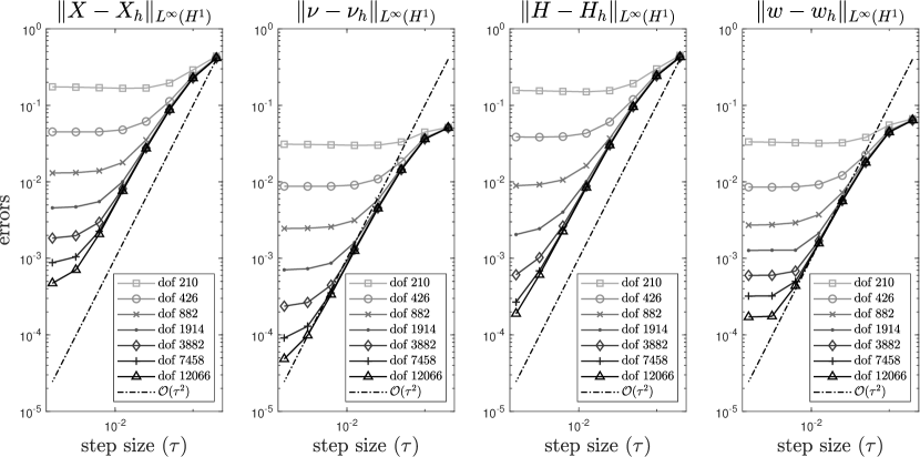
Figure 1: Temporal convergence of the algorithm (5.3) for forced MCF with $g(u)=u$, using BDF2 / quadratic ESFEM.

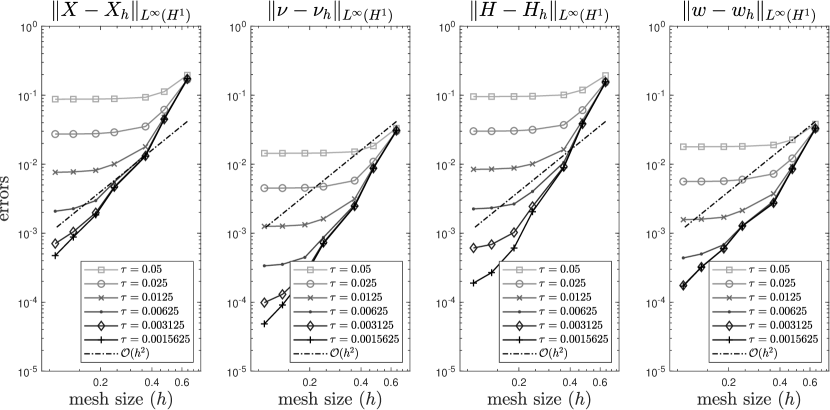
Figure 2: Spatial convergence of the algorithm (5.3) for forced MCF with $g(u)=u$, using BDF2 / quadratic ESFEM.

Using the algorithm in (5.3) with $2$-step BDF method and quadratic evolving surface FEM, we computed approximations to forced mean curvature flow, using $R_{0}=1$ and $R_{1}=2$, until time $T=1$. For our computations we used a sequence of time step sizes $\tau_{k}=\tau_{k-1}/2$ with $\tau_{0}=0.2$, and a sequence of initial meshes of mesh widths $h_{k}\approx 2^{-1/2}h_{k-1}$ with $h_{0}\approx 0.5$. The numerical experiments suggest that the step size restriction (6.1) is not required in practice.

In Figure 1 and 2 we report the errors between the exact and both numerical solutions for all four variables, i.e. the surface error, the errors in the dynamic variables $\nu$ and $H$, and the error in the PDE variable $u$. The logarithmic plots show the $L^{\infty}(H^{1})$ norm errors against the time step size $\tau$ in Figure 1, and against the mesh width $h$ in Figure 2. The lines marked with different symbols correspond to different mesh refinements and to different time step sizes in Figure 1 and 2, respectively.

In Figure 1 we can observe two regions: a region where the temporal discretization error dominates, matching to the $O(\tau^{2})$ order of convergence of our theoretical results, and a region, with small time step sizes, where the spatial discretization error dominates (the error curves flatten out). For Figure 2, the same description applies, but with reversed roles.

Both the temporal and spatial convergence, as shown by Figures 1 and 2, respectively, are in agreement with the theoretical convergence results of Theorem 4.1 and 6.1 (note the reference lines).

We have performed the same convergence experiments using algorithm (5.4), which, in view of Remarks 4.2 and 6.2, and the stability and convergence results of previous works [33, 29, 30, 28], should also have the same convergence properties as the algorithm (5.4). As Figures (3) and (4) (created analogously as Figure 1 and 2) illustrate, this expectation appears to be fulfilled.

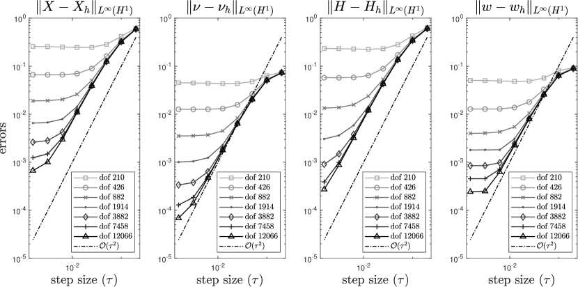
Figure 3: Temporal convergence of the algorithm (5.4) for forced MCF with $g(u)=u$, using BDF2 / quadratic ESFEM.

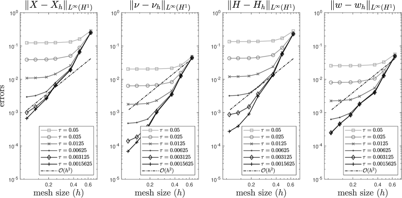
Figure 4: Spatial convergence of the algorithm (5.4) for forced MCF with $g(u)=u$, using BDF2 / quadratic ESFEM.

We have obtained similar convergence plots for the non-linear forcing term $g(u)=\tfrac{1}{2}u^{2}$ for both algorithms.

7.2 Tumour growth

We performed numerical experiments, using (5.3), on a well-known model for forced mean curvature flow from [2, Section 5]: The problem (7.1), with vector valued unknown $u=(u_{1},u_{2})$ and with a small parameter $\varepsilon=0.01$, models solid tumour growth, for further details we refer to [8, 9, 7] and [2]. Our results can be compared to those in these references, in particularly with those in [2].

The surface PDE system for $u=(u_{1},u_{2})$ describes the activator–depleted kinetics, and has diffusivity constants $1$ and $d=10$ for $u_{1}$ and $u_{2}$, respectively. The reaction term is given by, with $\gamma>0$,

$$F(u)=F(u_{1},u_{2})=\left(\begin{array}[]{c}\gamma\big{(}a-u_{1}+u_{1}^{2}u_{2}\big{)}\\ \gamma\big{(}b-u_{1}^{2}u_{2}\big{)}\end{array}\right),$$

while in the velocity law the non-linearity is given by

$$g(u)=g(u_{1},u_{2})=\delta\,u_{1}.$$

The parameters are chosen exactly as in [2, Table 5]: $d=10$, $a=0.1$, $b=0.9$, $\delta=0.1$, and $\epsilon=0.01$. The parameter $\gamma$ will be varied for different experiments.

The initial data for all of the presented experiments are obtained (exactly as in [2, Section 4.1.1 and Figure 8]) by integrating the reaction–diffusion system on the fixed unit sphere over the time interval $[0,5]$, with small random perturbations of the steady state $u_{1}=a+b$ and $u_{2}=b/(a+b)^{2}$ as initial data. Further initial values (for $i=1,\dotsc,q-1$) for high-order BDF methods are computed using a cascade of steps performed by the corresponding lower order methods.

To mitigate the stiffness of the non-linear term, the linear part of $F(u)$ is handled fully implicitly, while the non-linear parts of $F$, and the velocity law as well, are treated linearly implicitly using the extrapolation (5.2).

In Figure 5 and 6 we report on the evolution of the surface (and the approximated mean curvature and normal vector) and the component $u_{1}$ for parameters $\gamma=30$ and $\gamma=300$, respectively, at different times over the time interval $[5,8]$. In these plots the linear interpolation of the computed quadratic surface is plotted (since Matlab can only visualise polygonal objects). Figure 5 and 6 we present the surface evolution and the component $u_{1}$ of the surface PDE system (left-hand side columns) and the computed mean curvature $H_{h}$ and normal vector $\nu_{h}$ (right-hand side columns) at times $t=5,6,7,8$ (the rows from top to bottom), on a mesh with $3882$ nodes and time step size $\tau=0.0015625$. In particular the top rows show the initial data where the surface evolution is started. The obtained results for the surface evolution and the reaction–diffusion PDE system (left columns) match nicely (note the random effects in generating initial data) to previously reported results.

In spite of the smoothing effect of the mean curvature flow, for some more complicated examples it would be beneficial to use an algorithm which allows the tangential motion of the surface nodes, for example based on the DeTurck trick [19], or on the velocity law $v\cdot\nu=V$, e.g., [4, 5], or on ALE techniques [21, 31, 27]. However, in our experiments – both here and in [28] – this was not found necessary.

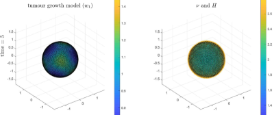
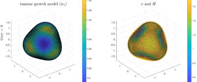
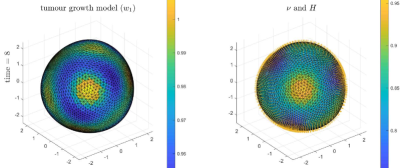
Figure 5: Evolution of the solution ($u_{1}$), normal vector and mean curvature for tumour growth model with $\gamma=30$ at time $t=5,6,7,8$; dof $3882$.

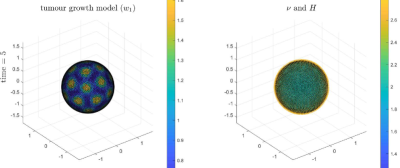
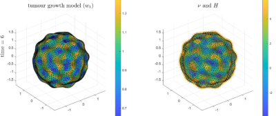
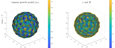
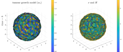
Figure 6: Evolution of the solution ($u_{1}$), normal vector and mean curvature for tumour growth model with $\gamma=300$ at time $t=5,6,7,8$; dof $3882$.

References

- [1] G. Akrivis and C. Lubich. Fully implicit, linearly implicit and implicit–explicit backward difference formulae for quasi-linear parabolic equations. Numer. Math., 131(4):713–735, 2015.
- [2] R. Barreira, C. M. Elliott, and A. Madzvamuse. The surface finite element method for pattern formation on evolving biological surfaces. J. Math. Biol., 63(6):1095–1119, 2011.
- [3] J. Barrett, K. Deckelnick, and V. Styles. Numerical analysis for a system coupling curve evolution to reaction diffusion on the curve. SIAM J. Numer. Anal., 55(2):1080–1100, 2017.
- [4] J. Barrett, H. Garcke, and R. Nürnberg. On the variational approximation of combined second and fourth order geometric evolution equations. SIAM J. Sci. Comput., 29(3):1006–1041, 2007.
- [5] J. Barrett, H. Garcke, and R. Nürnberg. On the parametric finite element approximation of evolving hypersurfaces in . J. Comput. Phys., 227(9):4281–4307, 2008.
- [6] J. Barrett, H. Garcke, and R. Nürnberg. Parametric finite element approximations of curvature driven interface evolutions. Handbook of Numerical Analysis, 21:275–423, 2020.
- [7] M. Chaplain, M. Ganesh, and I. Graham. Spatio-temporal pattern formation on spherical surfaces: numerical simulation and application to solid tumour growth. J. Math. Biol., 42(5):387–423, 2001.
- [8] E. J. Crampin, E. A. Gaffney, and P. K. Maini. Reaction and diffusion on growing domains: Scenarios for robust pattern formation. Bull. Math. Biol., 61(6):1093–1120, Nov 1999.
- [9] E. J. Crampin, E. A. Gaffney, and P. K. Maini. Mode-doubling and tripling in reaction-diffusion patterns on growing domains: a piecewise linear model. J. Math. Biol., 44(2):107–128, 2002.
- [10] K. Deckelnick, G. Dziuk, and C. M. Elliott. Computation of geometric partial differential equations and mean curvature flow. Acta Numerica, 14:139–232, 2005.
- [11] K. Deckelnick, C. Elliott, and V. Styles. Numerical diffusion-induced grain boundary motion. Interfaces Free Bound., 3(4):393–414, 2001.
- [12] A. Demlow. Higher–order finite element methods and pointwise error estimates for elliptic problems on surfaces. SIAM J. Numer. Anal., 47(2):805–807, 2009.
- [13] G. Dziuk. Finite elements for the Beltrami operator on arbitrary surfaces. in Partial differential equations and calculus of variations, Lecture Notes in Math., 1357, Springer, Berlin, pages 142–155, 1988.
- [14] G. Dziuk. An algorithm for evolutionary surfaces. Numer. Math., 58(1):603–611, 1990.
- [15] G. Dziuk and C. Elliott. Finite elements on evolving surfaces. IMA J. Numer. Anal., 27(2):262–292, 2007.
- [16] G. Dziuk and C. Elliott. Finite element methods for surface PDEs. Acta Numerica, 22:289–396, 2013.
- [17] K. Ecker. Regularity theory for mean curvature flow. Springer, Berlin, 2012.
- [18] C. Eilks and C. Elliott. Numerical simulation of dealloying by surface dissolution via the evolving surface finite element method. J. Comput. Phys., 227(23):9727–9741, 2008.
- [19] C. Elliott and H. Fritz. On approximations of the curve shortening flow and of the mean curvature flow based on the DeTurck trick. IMA J. Numer. Anal., 37(2):543–603, 2017.
- [20] C. M. Elliott and H. Fritz. On approximations of the curve shortening flow and of the mean curvature flow based on the DeTurck trick. IMA J. Numer. Anal., 37(2):543–603, 2017.
- [21] C. M. Elliott and C. Venkataraman. Error analysis for an ALE evolving surface finite element method. Numerical Methods for Partial Differential Equations, 31(2):459–499, 2015.
- [22] J. Erlebacher, M. Aziz, A. Karma, N. Dimitrov, and K. Sieradzki. Evolution of nanoporosity in dealloying. Nature, 410(6827):450, 2001.
- [23] J. Eyles, J. F. King, and V. Styles. A tractable mathematical model for tissue growth. arXiv:1907.06590, 2019.
- [24] P. Fife, J. Cahn, and C. Elliott. A free-boundary model for diffusion-induced grain boundary motion. Interfaces Free Bound., 3(3):291–336, 2001.
- [25] E. Hairer and G. Wanner. Solving Ordinary Differential Equations II. Stiff and Differential–Algebraic Problems. Springer, Berlin, Second edition, 1996.
- [26] G. Huisken. Flow by mean curvature of convex surfaces into spheres. J. Differential Geometry, 20(1):237–266, 1984.
- [27] B. Kovács. Computing arbitrary Lagrangian Eulerian maps for evolving surfaces. NMPDE, 2019. doi:10.1002/num.22340.
- [28] B. Kovács, B. Li, and C. Lubich. A convergent evolving finite element algorithm for mean curvature flow of closed surfaces. Numer. Math., 143:797–853, 2019.
- [29] B. Kovács, B. Li, C. Lubich, and C. Power Guerra. Convergence of finite elements on an evolving surface driven by diffusion on the surface. Numer. Math., 137(3):643–689, 2017.
- [30] B. Kovács and C. Lubich. Linearly implicit full discretization of surface evolution. Numer. Math., 140(1):121–152, 2018.
- [31] B. Kovács and C. Power Guerra. Higher–oder time discretizations with ALE finite elements for parabolic problems on evolving surfaces. IMA J. Numer. Anal., 38(1):460–494, 2018.
- [32] C. Lubich and D. Mansour. Variational discretization of wave equations on evolving surfaces. Math. Comp., 84(292):513–542, 2015.
- [33] C. Lubich, D. Mansour, and C. Venkataraman. Backward difference time discretization of parabolic differential equations on evolving surfaces. IMA J. Numer. Anal., 33(4):1365–1385, 2013.
- [34] P.-O. Persson and G. Strang. A simple mesh generator in MATLAB. SIAM Review, 46(2):329–345, 2004.
- [35] P. Pozzi and B. Stinner. Curve shortening flow coupled to lateral diffusion. Numer. Math., 135(4):1171–1205, 2017.
- [36] V. Styles. An evolving surface finite element method for the numerical solution of diffusion induced grain boundary motion. In Numerical Mathematics And Advanced Applications 2011, pages 469–477. Springer, Heidelberg, 2013.
- [37] S. W. Walker. The shape of things: a practical guide to differential geometry and the shape derivative. SIAM, Philadelphia, 2015.