Anti-Alignments – Measuring The Precision of Process Models and Event Logs

Abstract

Processes are a crucial artefact in organizations, since they coordinate the execution of activities so that products and services are provided. The use of models to analyse the underlying processes is a well-known practice. However, due to the complexity and continuous evolution of their processes, organizations need an effective way of analysing the relation between processes and models. Conformance checking techniques asses the suitability of a process model in representing an underlying process, observed through a collection of real executions. One important metric in conformance checking is to asses the precision of the model with respect to the observed executions, i.e., characterize the ability of the model to produce behavior unrelated to the one observed. In this paper we present the notion of anti-alignment as a concept to help unveiling runs in the model that may deviate significantly from the observed behavior. Using anti-alignments, a new metric for precision is proposed. In contrast to existing metrics, anti-alignment based precision metrics satisfy most of the required axioms highlighted in a recent publication. Moreover, a complexity analysis of the problem of computing anti-alignments is provided, which sheds light into the practicability of using anti-alignment to estimate precision. Experiments are provided that witness the validity of the concepts introduced in this paper.

1 Introduction

Relating observed and modelled process behavior is the lion’s share of conformance checking [9]. Observed behavior is often recorded in form of event logs, that store the footprints of process executions. Symmetrically, process models are representations of the underlying process, which can be automatically discovered or manually designed. With the aim of quantifying this relation, conformance checking techniques consider four quality dimensions: fitness, precision, generalization and simplicity [24]. For the first three dimensions, the alignment between a process model and an event log is of paramount importance, since it allows relating modeled and observed behavior [1].

Given a process model and a trace in the event log, an alignment provides the run in the model which mostly resembles the observed trace. When alignments are computed, the quality dimensions can be defined on top [1, 20]. In a way, alignments are optimistic: although observed behavior may deviate significantly from modeled behavior, it is always assumed that the least deviations are the best explanation (from the model’s perspective) for the observed behavior.

In this paper we present a somewhat symmetric notion to alignments, denoted as anti-alignments. Given a process model and a log, an anti-alignment is a run of the model that mostly deviates from any of the traces observed in the log. The motivation for anti-alignments is precisely to compensate the optimistic view provided by alignments, so that the model is queried to return highly deviating behavior that has not been seen in the log. In contexts where the process model should adhere to a certain behavior and not leave much room for exotic possibilities (e.g., banking, healthcare), the absence of highly deviating anti-alignments may be a desired property for a process model. Using anti-alignments one cannot only catch deviating behavior, but also use it to improve some of the current quality metrics considered in conformance checking. In this paper we highlight the strong relation of anti-alignments and the precision metric: a highly-deviating anti-alignment may be considered as a witness for a loss in precision. Current metrics for precision lack this ability of exploring the model behavior beyond what is observed in the log, thus being considered as short-sighted [2].

We cast the problem of computing anti-alignments as the satisfiability of a Boolean formula, and provide high-level techniques which can for instance compute the most deviating anti-alignment for a certain run length, or the shortest anti-alignment for a given number of deviations.

Anti-alignments are related to the completeness of the log; a log is complete if it contains all the behavior of the underlying process [28]. For incomplete logs, the alternatives for computing anti-alignments grow, making it difficult to tell the difference between behavior not observed but meant to be part of the process, and behavior not observed which is not meant to be part of the process. Since there exists already some metrics to evaluate the completeness of an event log (e.g., [36]), we assume event logs have a high level of completeness before they are used for computing anti-alignments. Notice that in presence of an incomplete event log, anti-alignments can be used to interactively complete it: an anti-alignment that is certified by the stake-holder as valid process behavior can be appended to the event log to make it more complete.

This work is an extension of recent publications related to anti-alignments: in [10] we established for the first time the notion of anti-alignments based on the Hamming distance, and proposed a simple metric to estimate precision. Then, the work in [30] elaborated the notion of anti-alignments, heuristically computing them for the Levenshtein distance by adapting the $A^{*}$ search technique, and proposed two new notions for trace-based and log-based precision, that can be combined to estimate precision of process models. However, as it was claimed recently in a survey paper advocating for properties precision metrics should have [26], it was not known the satisfiability of the properties for the aforementioned metrics.

The contributions of the paper with respect to our previous work are now enumerated.

• We show how anti-alignments can be computed in an optimal way for the Levenshtein distance, without increasing the complexity class of the problem. Moreover we relate the two available distance encodings (Hamming and Levenshtein), and show the implications of using each one for anti-alignment based precision.

• We adapt the precision metrics from [30] to not depend on a particular length defined apriori.

• We prove the adherence of one of the new metrics proposed in this paper to most of the properties in [26].

• A novel implementation is provided, with several improvements, which makes it able to deal with larger instances.

• A new evaluation section is reported, that show empirically the capabilities of the proposed technique for large and real-life instances.

The remainder of the paper is organized as follows: in the next section, a simple example is used to emphasize the importance of anti-alignments and its application to estimate precision is shown. Then in Section 3 the basic theory needed for the understanding of the paper is introduced. Section 4 provides the formal definition of anti-alignments, whilst Section 5 formalizes the encoding into SAT of the problem of computing anti-alignments. In Section 6, we define a new metric, based on anti-alignments, for estimating precision of process models. Experiments are reported in Section 7, and related work in Section 8. Section 9 concludes the paper and gives some hints for future research directions.

2 A Motivating Example

Let us use the example shown in Figure 1 for illustrating the notion of anti-alignment. The example was originally presented in [31], and in this paper we present a very abstract version of it in Figure 1(a): The modeled process describes a realistic transaction process within a banking context. The process contains all sort of monetary checks, authority notifications, and logging mechanisms. The process is initiated when a new transaction is requested, opening a new instance in the system and registering all the components involved. The second step is to run a check on the person (or entity) origin of the monetary transaction. Then, the actual payment is processed differently, depending of the payment modality chosen by the sender (cash, cheque and payment). Later, the receiver is checked and the money is transferred. Finally, the process ends registering the information, notifying it to the required actors and authorities, and emitting the corresponding receipt.

(a)

(b)

Figure 1: Example (adapted from [31]). (a) Initial process model, (b) Modified process model.

Assume that a log covering all the three possible variants (corresponding to the three possible payment methods) with respect of the model in Figure 1(a) is given. The three different variants for this log will be:

ort, cs, pcap, cr, tm, nct
ort, cs, pchp, cr, tm, nct
ort, cs, pep, cr, tm, nct

where we use the acronym for each one of the actions performed, e.g., ort stands for open and register transaction.

For this pair of model and log, most of the current metrics for precision (e.g., [2]) will rightly assess a very high precision. In fact, since no deviating anti-alignment can be obtained because every model run is in the log, the anti-alignment based precision metric from this paper will also assess a high (in our case, perfect) precision.

Now assume that we modify a bit the model, adding a loop around the alternative stages for the payment. Intuitively, this (malicious) modification in the process model may allow to pay several times although only one transfer will be done. The modified high-level overview is shown in Figure 1(b). The aforementioned metric for precision will not consider this modification as a severe one: the precision of the model with respect to the log will be very similar to the one for the model in Figure 1(a).

Remarkably, this modification in the process model comes with a new highly deviating anti-alignment denoting a run of the model that contains more than one iteration of the payment:

ort, cs, pcap, pchp, pchp, pep, pcap, cr, tm, nct

Clearly, this model execution where five payments have been recorded is possible in the process of Figure 1(b). Correspondingly, the precision of this model in describing the log of only three variants will be significantly lowered in the metric proposed in this paper, since the anti-alignment produced is very different from any of the three variants recorded in the event log.

3 Preliminaries

Definition 1 ((Labeled) Petri net)

A (labeled) Petri Net [21] is a tuple $N=\langle P,T,\mathcal{F},M_{0},M_{f},\Sigma,\lambda\rangle$, where $P$ is the set of places, $T$ is the set of transitions (with $P\cap T=\emptyset$), $\mathcal{F}:(P\times T)\cup(T\times P)\to\{0,1\}$ is the flow relation, $M_{0}$ is the initial marking, $M_{f}$ is the final marking, $\Sigma$ is an alphabet of actions and $\lambda:T\to\Sigma$ labels every transition by an action.

A marking is an assignment of a non-negative integer to each place. If $k$ is assigned to place $p$ by marking $M$ (denoted $M(p)=k$), we say that $p$ is marked with $k$ tokens. Given a node $x\in P\cup T$, its pre-set and post-set are denoted by ${{}^{\bullet}{x}}$ and ${{x}^{\bullet}}$ respectively.

A transition $t$ is enabled in a marking $M$ when all places in ${{}^{\bullet}{t}}$ are marked. When a transition $t$ is enabled, it can fire by removing a token from each place in ${{}^{\bullet}{t}}$ and putting a token to each place in ${{t}^{\bullet}}$. A marking $M^{\prime}$ is reachable from $M$ if there is a sequence of firings $t_{1}\ldots t_{n}$ that transforms $M$ into $M^{\prime}$, denoted by ${M}[t_{1}\ldots t_{n}\rangle{M^{\prime}}$. We define the language of $N$ as the set of full runs defined by $\mathcal{L}(N)\mathrel{:=}\{\lambda(t_{1})\ldots\lambda(t_{n})\mid{M_{0}}[t_{1}\ldots t_{n}\rangle{M_{f}}\}$. A Petri net is k-bounded if no reachable marking assigns more than $k$ tokens to any place. A Petri net is bounded if there exist a $k$ for which it is $k$-bounded. A Petri net is safe if it is 1-bounded. A bounded Petri net has an executable loop if it has a reachable marking $M$ and sequences of transitions $u_{1}\in T^{*}$, $u_{2}\in T^{+}$, $u_{3}\in T^{*}$ such that ${M_{0}}[u_{1}\rangle M[u_{2}\rangle M[u_{3}\rangle{M_{f}}$.

An event log is a collection of traces, where a trace may appear more than once. Formally:

Definition 2 (Event Log)

An event log $L$ (over an alphabet of actions $\Sigma$) is a multiset of traces $\sigma\in\Sigma^{*}$.

Process mining techniques aim at extracting from a log $L$ a process model $N$ (e.g., a Petri net) with the goal to elicit the process underlying a system ${\mathcal{S}}$. ${\mathcal{S}}$ is considered a language for the sake of comparison. By relating the behaviors of $L$, $\mathcal{L}(N)$ and ${\mathcal{S}}$, particular concepts can be defined [8]. A log is incomplete if ${\mathcal{S}}\setminus L\neq\emptyset$. A model $N$ fits log $L$ if $L\subseteq\mathcal{L}(N)$. A model is precise in describing a log $L$ if $\mathcal{L}(N)\setminus L$ is small. A model $N$ represents a generalization of log $L$ with respect to system ${\mathcal{S}}$ if some behavior in ${\mathcal{S}}\setminus L$ exists in $\mathcal{L}(N)$. Finally, a model $N$ is simple when it has the minimal complexity in representing $\mathcal{L}(N)$, i.e., the well-known Occam’s razor principle.

4 Anti-Alignments

The idea of anti-alignments is to seek in the language of a model $N$ what are the runs which differ considerably with all the observed traces. Hence, this is the opposite of the notion of alignments [1] which is central in process mining: for many tasks in conformance checking like process model repair or decision point analysis, one needs indeed to find the run which is the most similar to a given log trace [28]. In this paper, we are focusing on precision and for this, traces which are not similar to any observed trace in the log serve as witnesses for bad precision. All these notions anyway depend on a definition of distance between two traces (typically a model trace, i.e. a run of the model, and an observed log trace). We assume a given distance function $\mathit{dist}:\Sigma^{*}\times\Sigma^{*}\rightarrow[0,1]$ computable in polynomial time and such that

• for every $\gamma\in\Sigma^{*}$, $\mathit{dist}(\gamma,\gamma)=0$,

• for every $\sigma\in\Sigma^{*}$, $\mathit{dist}(\gamma,\sigma)$ converges to $1$ when $|\gamma|$ diverges to $\infty$.

Definition 3 (Anti-alignment)

For a distance threshold $m\in[0,1]$, an $m$-anti-alignment of a model $N$ w.r.t. a log $L$ is a full run $\gamma\in\mathcal{L}(N)$ such that $\mathit{dist}(\gamma,L)\geq m$, where $\mathit{dist}(\gamma,L)$ is defined as the $\min_{\sigma\in L}\mathit{dist}(\gamma,\sigma)$.

For the following examples, we show anti-alignments w.r.t. two possible choices of distance $\mathit{dist}$: Levenshtein’s distance and Hamming distance.

Definition 4 (Levenshtein’s edit distance $\mathit{dist}^{L}$)

Levenshtein’s edit distance $\mathit{dist}^{L}(\gamma,\sigma)$ between two traces $\gamma,\sigma\in\Sigma^{*}$ is based on the minimum number $n$ of deletions and insertions needed to transform $\gamma$ to $\sigma$. In order to get a normalized distance between 0 and 1, we define Levenshtein’s edit distance $\mathit{dist}^{L}(\gamma,\sigma)=\frac{n}{\max(1,|\gamma|+|\sigma|)}$.

Example 1

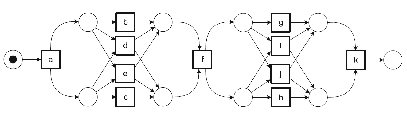
$$L=\{\begin{array}[t]{@{}l@{}}\langle a,b,c,f,g,h,k\rangle,\\ \langle a,c,b,f,g,h,k\rangle,\\ \langle a,c,b,f,h,g,k\rangle,\\ \langle a,b,c,f,h,g,k\rangle,\\ \langle a,e,f,i,k\rangle,\\ \langle a,d,f,g,h,k\rangle,\\ \langle a,e,f,h,g,k\rangle\}\,,\end{array}$$

Figure 2: A process model (taken from [29]) and an event log. The full run $\langle a,b,c,f,i,k\rangle$ is a $\frac{3}{13}$-anti-alignment for Levenshtein’s distance and a $\frac{3}{7}$-anti-alignment for Hamming distance.

Consider the Petri net and log shown in Figure 2. With Levenshtein’s distance, the full run $\langle a,b,c,f,i,k\rangle$ is at distance $\frac{3}{13}$ from the log trace $\langle a,b,c,f,g,h,k\rangle$ (two deletions and one insertion). It is at larger distance from the other log traces. Therefore, it is a $\frac{3}{13}$-anti-alignment.

Another interesting choice is Hamming distance. It is in general less informative than Levenshtein’s distance for relating observed and modelled behavior, but it has the interest of being very simple to compute. Variants of Hamming distance can also provide good compromises. In Sections 5 and 6, we will show how to efficiently compute anti-alignments for Hamming distance using SAT solvers.

Definition 5 (Hamming distance $\mathit{dist}^{H}$)

For two traces $\gamma=\gamma_{1}\dots\gamma_{n}$ and $\sigma=\sigma_{1}\dots\sigma_{n}$, of same length $n>0$, define $\mathit{dist}^{H}(\gamma,\sigma)\mathrel{:=}\frac{1}{n}\cdot\big{|}\big{\{}i\in\{1\dots n\}\mid\gamma_{i}\neq\sigma_{i}\big{\}}\big{|}$. For $\gamma$ longer than $\sigma$, we define $\mathit{dist}^{H}(\gamma,\sigma)\mathrel{:=}\mathit{dist}^{H}(\gamma,\sigma\cdot w^{|\gamma|-|\sigma|})$, where $w\not\in\Sigma$ is a special padding symbol ($w$ for ‘wait’); we proceed symmetrically when $\gamma$ is shorter than $\sigma$.

Lemma 1

Observe that, for every $\gamma$ and $\sigma$ (assuming one of them at least is nonempty), $\mathit{dist}^{L}(\gamma,\sigma)\leq\mathit{dist}^{H}(\gamma,\sigma)$.

Proof

Assume w.l.o.g. $0<|\gamma|<|\sigma|$. Let $n\mathrel{:=}\big{|}\big{\{}i\in\{1\dots|\gamma|\}\mid\gamma_{i}\neq\sigma_{i}\big{\}}\big{|}$. We have, $\mathit{dist}_{H}(\gamma,\sigma)=\frac{n+|\sigma|-|\gamma|}{|\sigma|}$. We have also $\mathit{dist}_{L}(\gamma,\sigma)\leq\frac{2n+|\sigma|-|\gamma|}{|\gamma|+|\sigma|}$ because one way to transform $\gamma$ to $\sigma$ is to replace $\gamma_{i}$ by $\sigma_{i}$ (one deletion and one insertion) at each position $i\leq|\gamma|$ where they differ ($2n$ editions), and then to insert the letters $\sigma_{|\gamma|+1}\dots\sigma_{|\sigma|}$ ($|\sigma|-|\gamma|$ editions). It remains to see that $n\leq|\gamma|$, which implies

$$n(|\sigma|-|\gamma|) \leq |\gamma|(|\sigma|-|\gamma|)$$

$$n|\sigma| \leq |\gamma|(n+|\sigma|-|\gamma|)$$

$$n|\sigma|+(n+|\sigma|-|\gamma|)|\sigma| \leq |\gamma|(n+|\sigma|-|\gamma|)+(n+|\sigma|-|\gamma|)|\sigma|$$

$$(2n+|\sigma|-|\gamma|)|\sigma| \leq (|\gamma|+|\sigma|)(n+|\sigma|-|\gamma|)$$

$$\frac{2n+|\sigma|-|\gamma|}{|\gamma|+|\sigma|} \leq \frac{(n+|\sigma|-|\gamma|)}{|\sigma|}$$

$$\mathit{dist}^{L}(\gamma,\sigma) \leq \mathit{dist}^{H}(\gamma,\sigma)\;.$$

∎

Example 2

Consider the Petri net and log shown in Figure 2. With Hamming distance, the full run $\gamma=\langle a,b,c,f,i,k\rangle$ is at distance $\frac{3}{7}$ from the log trace $\sigma=\langle a,b,c,f,g,h,k\rangle$ ($i$ and $k$ do not match with $g$ and $h$, and $\gamma$ is shorter than $\sigma$, which counts for the third mismatch). It is at larger distance from the other log traces. Therefore, it is a $\frac{3}{7}$-anti-alignment.

Lemma 2

For every log $L$ and finite model $N$, we have:

1. if the model has finitely many full runs, then there exists (at least) one maximal anti-alignment $\gamma$ of $N$ w.r.t. $L$, i.e. $\gamma$ that maximizes the distance $\mathit{dist}(\gamma,L)$;

2. if the model has infinitely many full runs, then there exist anti-alignments $\gamma$ with $\mathit{dist}(\gamma,L)$ arbitrarily close to $1$. Yet, there may not exist any $1$-anti-alignment, i.e. there is no guarantee that the limit $\mathit{dist}(\gamma,L)=1$ is reached for any $\gamma$.

Proof

If the model has finitely many full runs, then one of them must be a maximal anti-alignment.

Conversely, if $N$ is finite and has infinitely many runs, then there must exist arbitrary long full runs; more formally, there exists an infinite sequence of full runs $(\gamma_{i})_{i\in\mathbb{N}}$ of strictly increasing length. For every $\sigma\in L$, the sequence of $(\mathit{dist}(\gamma_{i},\sigma))_{i\in\mathbb{N}}$ converges to $1$. Since there are finitely many $\sigma\in L$, $(\min_{\sigma\in L}\mathit{dist}(\gamma_{i},\sigma))_{i\in\mathbb{N}}$ converges to $1$ as well. ∎

Maximal anti-alignments will be used in Section 6 to define our precision metric. The case of models with executable loops will be discussed in Subsection 6.1.1.

Lemma 3

The problem of deciding, given a finite model $N$ and a log $L$, whether there exists a $0$-anti-alignment of $N$ w.r.t. $L$, has the same complexity as reachability for Petri nets.

Proof

This is equivalent to checking whether $\mathcal{L}(N)\neq\emptyset$, i.e. whether $M_{f}$ is reachable from $M_{0}$.∎

By definition, a $0$-anti-alignment of $N$ w.r.t. $L$ is a full run $\gamma\in\mathcal{L}(N)$ satisfying the trivial inequality $\mathit{dist}(\gamma,L)\geq 0$. The same problem with a strict inequality is also of interest. We will need it in Section 6.1.1.

Lemma 4

The problem of deciding, given a finite model $N$ and a log $L$, whether there exists a full run $\gamma\in\mathcal{L}(N)$ satisfying $\mathit{dist}(\gamma,L)>0$ (or equivalently deciding if $\mathcal{L}(N)\not\subseteq L$), has the same complexity as reachability for Petri nets.

Proof

The reachability problem reduces to the existence of a full run $\gamma\in\mathcal{L}(N)$ satisfying $\mathit{dist}(\gamma,\emptyset)>0$: indeed $\mathit{dist}(\gamma,\emptyset)=1$ for every $\gamma$.

Figure 3: A deterministic Petri net representing the log $L=\{\langle a\rangle,\langle a,b\rangle,\langle a,a\rangle,\langle b\rangle\}$, for the alphabet of actions $\Sigma=\{a,b\}$. Place $p_{esc}$ is reached only by the runs which do not appear in the log.

Conversely, deciding if $\mathcal{L}(N)\not\subseteq L$ reduces to deciding reachability of $M_{f}\cup\{p_{esc}\}$ in the synchronous product of $N$ with a deterministic Petri net which represents as a tree the log traces sharing their common prefixes, and, from the leaves, marks a sink place $p_{esc}$, as illustrated in Figure 3. Hence, every full run $\gamma$ of $N$, when synchronized with the Petri net representation of the log $L$, leads to a marking of the form $M_{f}\cup\{p\}$, and $p=p_{esc}$ iff $\gamma\not\in L$. ∎

The problem of reachability in Petri nets is known to be decidable, but non-elementary [12].

Yet, the complexity drops to NP if a bound is given on the length of the anti-alignment.

Lemma 5

The problem of deciding, for a Petri net $N$, a log $L$, a rational distance threshold $m\in\mathbb{Q}$ and a bound $n\in\mathbb{N}$, if there exists a $m$-anti-alignment $\gamma$ such that $|\gamma|\leq n$, is NP-complete. We assume that $n$ is encoded in unary.

Proof

The problem is clearly in NP: checking that a run $\gamma$ is a $m$-anti-alignment of $N$ w.r.t. $L$ takes polynomial time (remember that we consider distance functions computable in polynomial time).

For NP-hardness, we propose a reduction from the problem of reachability of a marking $M_{f}$ in a 1-safe acyclic Petri net $N$, known to be NP-complete [25, 11]. Notice that, since $N$ is acyclic, each transition can fire only once; hence, the length of the firing sequences of $N$ is bounded by the number of transitions $|T|$. Finally, $M_{f}$ is reachable in $N$ iff there exists a $\gamma$ of length less or equal to $|T|$ which is a $0$-anti-alignment of $N$ (with $M_{f}$ as final marking) w.r.t. the empty log. ∎

5 SAT-encoding of Anti-Alignments

In this section, we give hints on how SAT solvers can help to find anti-alignments. We detail the construction of a SAT formula $\Phi^{n}_{m}(N,L)$, where $N$ is a Petri net, $L$ a log, $n$ and $m$ two integers. This formula will be used in the search of anti-alignments of $N$ w.r.t. $L$ for Hamming distance (see Section 5.3 for the encoding using the Levenshtein distance). The formula $\Phi^{n}_{m}(N,L)$ characterizes precisely the full runs $\gamma=\lambda(t_{1})\dots\lambda(t_{n})\in\mathcal{L}(N)$ of $N$ of length $n$ which differs in at least $m$ positions with every log trace in $L$.

5.1 Coding $\Phi^{n}_{m}(N,L)$ Using Boolean Variables

The formula $\Phi^{n}_{m}(N,L)$ is coded using the following Boolean variables:

• $\tau_{i,t}$ for $i=1\dots n$, $t\in T$ (remind that $w$ is the special symbol used to pad the log traces, see Definition 5) means that transition $t_{i}=t$.

• $m_{i,p}$ for $i=0\dots n$, $p\in P$ means that place $p$ is marked in marking $M_{i}$ (remind that we consider only safe nets, therefore the $m_{i,p}$ are Boolean variables).

• $\delta_{i,\sigma,k}$ for $i=1\dots n$, $\sigma\in L$, $k=1,\dots,m$ means that the $k$^th mismatch with the observed trace $\sigma$ is at position $i$.

The total number of variables is $O(n\times(|T|+|P|+|L|\times m))$.

Let us decompose the formula $\Phi^{n}_{m}(N,L)$.

• The fact that $\gamma=\lambda(t_{1})\dots\lambda(t_{n})\in\mathcal{L}(N)$ is coded by the conjunction of the following formulas:

  • Initial marking:

    $$\left(\bigwedge_{p\in M_{0}}m_{0,p}\right)\land\left(\bigwedge_{p\in P\setminus M_{0}}\lnot m_{0,p}\right)$$

  • Final marking:

    $$\left(\bigwedge_{p\in M_{f}}m_{n,p}\right)\land\left(\bigwedge_{p\in P\setminus M_{f}}\lnot m_{n,p}\right)$$

  • One and only one $t_{i}$ for each $i$:

    $$\bigwedge_{i=1}^{n}\bigvee_{t\in T}(\tau_{i,t}\land\bigwedge_{t^{\prime}\in T}\lnot\tau_{i,t^{\prime}})$$

  • The transitions are enabled when they fire:

    $$\bigwedge_{i=1}^{n}\bigwedge_{t\in T}(\tau_{i,t}\implies\bigwedge_{p\in{{}^{\bullet}{t}}}m_{{i-1},p})$$

  • Token game (for safe Petri nets):

    $$\bigwedge_{i=1}^{n}\bigwedge_{t\in T}\bigwedge_{p\in{{t}^{\bullet}}}(\tau_{i,t}\implies m_{i,p})$$

    $$\bigwedge_{i=1}^{n}\bigwedge_{t\in T}\bigwedge_{p\in{{}^{\bullet}{t}}\setminus{{t}^{\bullet}}}(\tau_{i,t}\implies\lnot m_{i,p})$$

    $$\bigwedge_{i=1}^{n}\bigwedge_{t\in T}\bigwedge_{p\in P,p\not\in{{}^{\bullet}{t}},p\not\in{{t}^{\bullet}}}(\tau_{i,t}\implies(m_{i,p}\iff m_{{i-1},p}))$$

• Now, the constraint that $\gamma$ deviates from the observed traces (for every $\sigma\in L$, $\mathit{dist}(\gamma,\sigma)\geq m$) is coded as:

  $$\bigwedge_{\sigma\in L}\bigwedge_{k=1}^{m}\bigvee_{i=1}^{n}\delta_{i,\sigma,k}$$

  with the $\delta_{i,\sigma,k}$ correctly affected w.r.t. $\lambda(t_{i})$ and $\sigma_{i}$:

  $$\bigwedge_{\sigma\in L}\bigwedge_{k=1}^{m}\bigwedge_{i=1}^{n}\Big{(}\delta_{i,\sigma,k}\iff\bigvee_{t\in T,\ \lambda(t)\neq\sigma_{i}}\tau_{i,t}\Big{)}$$

  and that for $k\neq k^{\prime}$, the $k$^th and $k^{\prime}$^th mismatch correspond to different $i$’s (i.e. a given mismatch cannot serve twice):

  $$\bigwedge_{\sigma\in L}\bigwedge_{i=1}^{n}\bigwedge_{k=1}^{m-1}\bigwedge_{k^{\prime}=k+1}^{m}\lnot(\delta_{i,\sigma,k}\land\delta_{i,\sigma,k^{\prime}})$$

5.2 Size of the Formula

In the end, the first part of the formula ($\gamma=\lambda(t_{1})\dots\lambda(t_{n})\in\mathcal{L}(N)$) is coded by a Boolean formula of size $O(n\times|T|\times|N|)$, with $|N|\mathrel{:=}|T|+|P|$.

The second part of the formula (for every $\sigma\in L$, $\mathit{dist}(\gamma,\sigma)\geq m$) is coded by a Boolean formula of size $O(n\times m^{2}\times|L|\times|T|)$.

The total size for the coding of the formula $\Phi^{n}_{m}(N,L)$ is

$$O\left(n\times|T|\times\big{(}|N|+m^{2}\times|L|\big{)}\right)\,.$$

5.3 SAT-encoding of Anti-Alignments for Levenshtein’s Edit Distance

Our SAT-encoding of anti-alignments for Levenshtein’s edit distance uses the same boolean variables as the SAT-encoding of anti-alignments for Hamming distance of the previous section, completed with $\delta$ variables used to encode the edit distance.

Our encoding is based on the same relations that are used by the classical dynamic programming recursive algorithm for computing the edit distance between two words $u=\langle u_{1},\dots,u_{n}\rangle$ and $v=\langle v_{1},\dots,v_{m}\rangle$:

$$\left\{\begin{array}[]{ll}\mathit{dist}(\langle u_{1},\dots,u_{i}\rangle,\epsilon)=i\\ \mathit{dist}(\epsilon,\langle v_{1},\dots,v_{j}\rangle)=j\\ \mathit{dist}(\langle u_{1},\dots,u_{i+1}\rangle,\langle v_{1},\dots,v_{j+1}\rangle)=\\ \qquad\left\{\begin{array}[]{l @{\quad\mbox{ if }} l}\mathit{dist}(\langle u_{1},\dots,u_{i}\rangle,\langle v_{1},\dots,v_{j}\rangle)&u_{i+1}=v_{j+1}\\ \begin{array}[]{l@{}l}1+\min(&\mathit{dist}(\langle u_{1},\dots,u_{i+1}\rangle,\langle v_{1},\dots,v_{j}\rangle),\\ &\mathit{dist}(\langle u_{1},\dots,u_{i}\rangle,\langle v_{1},\dots,v_{j+1}\rangle))\end{array}&u_{i+1}\not=v_{j+1}\end{array}\right.\end{array}\right.$$

We encode this computation in a SAT formula $\phi$ over variables $\delta_{i,j,d}$, for $i=0,\dots,n$, $j=0,\dots,m$ and $d=0,\dots,n+m$. Formula $\phi$ will have exactly one solution, in which each variable $\delta_{i,j,d}$ is true iff $u_{1}\dots u_{i}$ and $v_{1}\dots v_{j}$ differ by at least $d$ editions.

In order to test equality between the $u_{i}$ and $v_{j}$, we use variables $\lambda_{i,a}$ and $\lambda^{\prime}_{j,a}$, for $i=0,\dots,n$, $j=0,\dots,m$ and $a\in\Sigma$, and we set their value such that $\lambda_{i,a}$ is true iff $u_{i}=a$, and $\lambda^{\prime}_{j,a}$ is true iff $v_{j}=a$. Hence, the test $u_{i+1}=v_{j+1}$ becomes in our formulas: $\bigvee_{a\in\Sigma}(\lambda_{i+1,a}\wedge\lambda^{\prime}_{j+1,a})$. For readability of the formulas, we refer to this coding by $[u_{i+1}=v_{j+1}]$. We also write similarly $[u_{i+1}\neq v_{j+1}]$.

In the following, we describe the different clauses of the formula $\phi$ of our SAT encoding of the edit distance.

$$\textstyle\delta_{0,0,0}\quad\land\quad\bigwedge_{d>0}\neg\delta_{0,0,d}$$ (1)

$$\textstyle\bigwedge_{d}\bigwedge_{i=0}^{n}\quad(\delta_{i+1,0,d+1}\Leftrightarrow\delta_{i,0,d})$$ (2)

$$\textstyle\bigwedge_{d}\bigwedge_{j=0}^{n}\quad(\delta_{0,j+1,d+1}\Leftrightarrow\delta_{0,j,d})$$ (3)

$$\textstyle\bigwedge\limits_{d}\bigwedge\limits_{i=0}^{n}\bigwedge\limits_{j=0}^{n}\quad[u_{i+1}=v_{j+1}]\Rightarrow(\delta_{i+1,j+1,d}\Leftrightarrow\delta_{i,j,d})$$ (4)

$$\textstyle\bigwedge\limits_{d}\bigwedge\limits_{i=0}^{n}\bigwedge\limits_{j=0}^{n}\quad[u_{i+1}\neq v_{j+1}]\Rightarrow(\delta_{i+1,j+1,d+1}\Leftrightarrow(\delta_{i+1,j,d}\wedge\delta_{i,j+1,d}))\qquad$$ (5)

Example 3

At instants $i=1$ and $j=1$ of words $u=\langle s,g,c\rangle$ and $v=\langle s,b,c,a\rangle$, the letters are the same, then, by (4), the distance is only higher or equal to 0 : $(u_{1}=v_{1})\Rightarrow(\delta_{1,1,0}\Leftrightarrow\delta_{0,0,0})$.

However at instants $i=2$ and $j=2$, the letters $u_{2}$ and $v_{2}$ are different. A step before, $\delta_{1,2,1}$ and $\delta_{2,1,1}$ are true because of the length of the subwords. Then, by (5), the distance at instants $i=2$ and $j=2$ is higher or equal to 2 : $\delta_{2,2,2}$. The result is understandable because the edit distance costs the deletion of $g$ and the addition of $b$ to transform $u$ to $v$.

In order to insert this encoding of Leventshein’s edit distance into our formulas for anti-alignments, we need to compute the edit distance between the expected anti-alignment and every trace of the log, which requires to use variables $\delta_{i,\sigma,j,k}$ for $i=0\dots n$, $\sigma\in L$, $j=0\dots|\sigma|$, $k=0,\dots,\max(n,|\sigma|)$ to represent the fact that $u_{1}\dots u_{i}$ and $v_{1}\dots v_{j}$ differ by at least $k$ editions.

5.4 Solving the Formula in Practice

In practice, the coding of the formula $\Phi^{n}_{m}(N,L)$ can be done using the Boolean variables $\tau_{i,t}$, $m_{i,p}$ and $\delta_{i,\sigma,k}$.

Then we need to transform the formula in conjunctive normal form (CNF) in order to pass it to the SAT solver. We use Tseytin’s transformation [27] to get a formula in conjunctive normal form (CNF) whose size is linear in the size of the original formula. The idea of this transformation is to replace recursively the disjunctions $\phi_{1}\lor\dots\lor\phi_{n}$ (where the $\phi_{i}$ are not atoms) by the following equivalent formula:

$$\exists x_{1},\dots,x_{n}\quad\left\{\begin{array}[]{ll}&x_{1}\lor\dots\lor x_{n}\\ \land&x_{1}\implies\phi_{1}\\ \land&\dots\\ \land&x_{n}\implies\phi_{n}\end{array}\right.$$

where $x_{1},\dots,x_{n}$ are fresh variables.

In the end, the SAT solver tells us if there exists a run $\gamma=\lambda(t_{1})\dots\lambda(t_{n})\in\mathcal{L}(N)$ which differs by at least $m$ editions with every observed trace $\sigma\in L$. If a solution is found, we extract the run $\gamma$ using the values assigned by the SAT solver to the Boolean variables $\tau_{i,t}$.

6 Using Anti-Alignments to Estimate Precision

In this section we show how to use anti-alignments to estimate precision of process models. Remarkably, we show how to modify the definitions of [10, 30] so that the new metric does not depend on a predefined length. In Section 6.2 we dive into the adherence of the metric with respect to a recent proposal for properties of precision metrics [26].

6.1 Precision

Our precision metric is an adaptation of our previous versions presented in [10, 30]. It relies on anti-alignments to find the model run that is as distant as possible to the log traces. Like anti-alignments, the definition of precision is parameterized by a distance $\mathit{dist}$. In the examples, we will specify each time if we use Levenshtein’s edit distance (Definition 4) or Hamming distance (Definition 5).

Definition 6 (Precision)

Let $L$ be an event log and $N$ a model. We define precision as follows:

$$P_{aa}(N,L)\mathrel{:=}1-\sup_{\gamma\in\mathcal{L}(N)}\mathit{dist}(\gamma,L)\,.$$

For instance, consider the model and log shown in Figure 2. With Levenshtein’s distance, the full run $\langle a,b,c,f,i,k\rangle$ is a maximal anti-alignment. It is at distance $\frac{3}{13}$ to any of the log traces, and hence $P_{aa}(N,L)=1-\frac{3}{13}=0.77$.

6.1.1 Handling Process Models with Loops

Notice that a model with arbitrary long runs (i.e., a process model that contains loops) may cause the formula in Definition 6 to converge to 0. This is a natural artifact of comparing a finite language (the event log), with a possibly infinite language (the process model). Since process models in reality contain loops, an adaptation of the metric is done in this section, so that it can also handle this type of models without penalizing severely the loops.

Definition 7 (Precision for Models with Loops)

Let $L$ be an event log and $N$ a model. We define $\epsilon$-precision as follows:

$$P_{aa}^{\epsilon}(N,L)\mathrel{:=}1-\sup_{\gamma\in\mathcal{L}(N)}\frac{\mathit{dist}(\gamma,L)}{(1+\epsilon)^{|\gamma|}}$$

with some $\epsilon\geq 0$ which is a parameter of this definition.

Informally, the formula computes the anti-alignment that provides maximal distance with any trace in the log, and at the same time tries to minimize its length. The penalization for the length is parametrized over the $\epsilon$. Observe that $P_{aa}^{0}(N,L)$ is precisely the precision $P_{aa}(N,L)$ of Definition 6. By making Definition 7 not dependant on a predefined length, it deviates from the log-based precision metrics defined in previous work [10, 30].

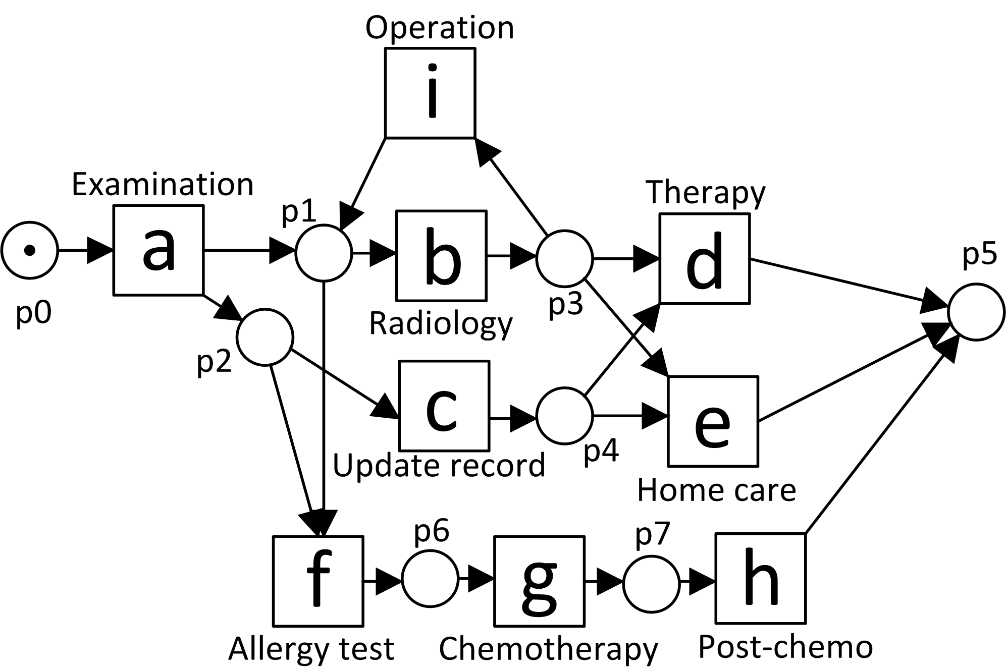
Figure 4: Example from [2]

Let us now consider the model of Figure 4, and the log $L=[\langle a\rangle,\langle a,b,c,d\rangle,\langle a,f,g,h\rangle,\langle a,b,i,b,c,d\rangle]$. Assume that $\epsilon=0.05$. A possible anti-alignment is $\gamma_{1}=\langle a,c,b,e\rangle$ which is at least at Levenshtein’s distance $\frac{1}{2}$ to any of the log traces. For $\gamma_{1}$ the value of the formula is $1-\frac{\frac{1}{2}}{(1.05)^{4}}=0.589$. Another possible anti-alignment is $\gamma_{2}=\langle a,c,b,i,b,i,b,i,b,i,b,e\rangle$ which is at least at distance $\frac{10}{18}$ to any of the log traces. For $\gamma_{2}$ the value of the formula is $1-\frac{\frac{10}{18}}{(1.05)^{12}}=0.691$. Hence, since the anti-alignment that maximizes the second term of the formula is $\gamma_{1}$, the precision computed is $P_{aa}^{0.05}(N,L)=0.589$. If instead, $\epsilon$ is set to a lower value, e.g., $\epsilon=0.02$, the corresponding value of the formula for the anti-alignment $\langle a,c,b,i,b,i,b,i,b,i,b,i,b,i,b,i,b,e\rangle$ will be the mainimal, and therefore it will be selected as the anti-alignment resulting in $P_{aa}^{0.02}(N,L)=0.533$.

6.1.2 Computing $P_{aa}^{\epsilon}$

By incorporating the $\epsilon$ parameter in the definition of precision, now the metric can deal with models containing loops without predefining the length of the anti-alignment. In this section we show that the proposed extension is well-defined and can be computed, and provide some complexity results of the algorithms involved.

Lemma 6

For every finite model $N$, log $L$ and $\epsilon>0$, the supremum in the definition of $P_{aa}^{\epsilon}$ is reached, i.e. there exists a full run $\gamma\in\mathcal{L}(N)$ such that $P_{aa}^{\epsilon}(N,L)=1-\frac{\mathit{dist}(\gamma,L)}{(1+\epsilon)^{|\gamma|}}$.

Proof

Two cases have to be distinguished: if $\mathcal{L}(N)\subseteq L$, then the supremum equals $0$, is obviously reached by any $\gamma\in\mathcal{L}(N)$, and $P_{aa}^{\epsilon}(N,L)=1$; otherwise, let $\gamma_{0}\in\mathcal{L}(N)\setminus L$ and let $m\mathrel{:=}\frac{\mathit{dist}(\gamma_{0},L)}{(1+\epsilon)^{|\gamma_{0}|}}$; we show that the supremum in the definition of $P_{aa}^{\epsilon}$ becomes now a maximum over a finite set of runs, bounded by a given length $n$ that depends on $m$ and $\epsilon$:

$$\sup_{\gamma\in\mathcal{L}(N)}\frac{\mathit{dist}(\gamma,L)}{(1+\epsilon)^{|\gamma|}}=\max_{\gamma\in\mathcal{L}(N),|\gamma|\leq n}\frac{\mathit{dist}(\gamma,L)}{(1+\epsilon)^{|\gamma|}}\,,$$

with $n\mathrel{:=}\left\lfloor\frac{-\log m}{\log(1+\epsilon)}\right\rfloor$. Indeed, for every $\gamma$ strictly longer than $n$, we have $\frac{\mathit{dist}(\gamma,L)}{(1+\epsilon)^{|\gamma|}}<\frac{1}{(1+\epsilon)^{n}}=\exp(-n\cdot\log(1+\epsilon))\leq\exp(\log m)=m$, which also shows that $|\gamma_{0}|\leq n$. Hence $\gamma_{0}$ is considered in our $\max$, and then $\max\limits_{\gamma\in\mathcal{L}(N),|\gamma|\leq n}\frac{\mathit{dist}(\gamma,L)}{(1+\epsilon)^{|\gamma|}}\geq m>\sup\limits_{\gamma\in\mathcal{L}(N),|\gamma|>n}\frac{\mathit{dist}(\gamma,L)}{(1+\epsilon)^{|\gamma|}}$. ∎

Lemma 6 gives us the key for an algorithm to compute $P_{aa}^{\epsilon}$.

Algorithm 1

Algorithm for computing $P_{aa}^{\epsilon}(N,L)$:

• if $\mathcal{L}(N)\not\subseteq L$, then

  • select $\gamma_{0}\in\mathcal{L}(N)\setminus L$

  • let $m\mathrel{:=}\frac{\mathit{dist}(\gamma_{0},L)}{(1+\epsilon)^{|\gamma_{0}|}}$

  • explore the reachability graph of $N$ until depth $n\mathrel{:=}\left\lfloor\frac{-\log m}{\log(1+\epsilon)}\right\rfloor$ and return $1-\max_{\gamma\in\mathcal{L}(N),|\gamma|\leq n}\frac{\mathit{dist}(\gamma,L)}{(1+\epsilon)^{|\gamma|}}$;

• else return $1$ (the model has perfect precision).

The correctness of this algorithm follows directly from Lemma 6. Its complexity resides essentially in the initial test, which corresponds to simply deciding if $P_{aa}^{\epsilon}(N,L)<1$, whose complexity is given by the following lemma:

Lemma 7

The problem of deciding, for a finite model $N$ and a log $L$, if $P_{aa}^{\epsilon}(N,L)<1$, is equivalent to deciding reachability in Petri nets.

Proof

We simply observe that $P_{aa}^{\epsilon}(N,L)<1$ iff $\mathcal{L}(N)\not\subseteq L$. Deciding this is equivalent to deciding reachability in Petri nets, as showed in Lemma 4. ∎

However, in practice, one would generally skip the first check and jump directly to the exploration until some depth $n$, possibly computed form a given threshold $m$, like the one given by the $\gamma_{0}$ in Algorithm 1. Notice that the algorithm explores less deep (i.e. $n$ is smaller) when $m$ is large (close to 1), i.e. $\gamma_{0}$ is close to the optimal anti-alignment. We can summarize this with the following variation of Algorithm 1:

Algorithm 2

Algorithm for estimating $P_{aa}^{\epsilon}(N,L)$ using a threshold $0<m\leq 1$ as input:

• explore the reachability graph of $N$ until depth $n\mathrel{:=}\left\lfloor\frac{-\log m}{\log(1+\epsilon)}\right\rfloor$

• if the exploration finds a full run $\gamma\in\mathcal{L}(N)\setminus L$

• then output “$P_{aa}^{\epsilon}(N,L)=1-\max_{\gamma\in\mathcal{L}(N),|\gamma|\leq n}\frac{\mathit{dist}(\gamma,L)}{(1+\epsilon)^{|\gamma|}}$”

• else output “$P_{aa}^{\epsilon}(N,L)\geq 1-m$”.

Lemma 8

For any fixed $\epsilon>0$, the problem of deciding, for a finite model $N$, a log $L$ and a rational constant $m>0$, if $P_{aa}^{\epsilon}(N,L)<1-m$, is NP-complete.

Proof

The proof is similar to the one of Lemma 6; here, the bound $m$ is given directly, and we have the same equality

$$\sup_{\gamma\in\mathcal{L}(N)}\frac{\mathit{dist}(\gamma,L)}{(1+\epsilon)^{|\gamma|}}=\max_{\gamma\in\mathcal{L}(N),|\gamma|\leq n}\frac{\mathit{dist}(\gamma,L)}{(1+\epsilon)^{|\gamma|}}\,,$$

with $n\mathrel{:=}\left\lfloor\frac{-\log m}{\log(1+\epsilon)}\right\rfloor$. This means, in order to check that $P_{aa}^{\epsilon}(N,L)<1-m$, it suffices to guess a full run $\gamma$ of length $|\gamma|\leq n$, where $n$ depends linearly on the size of the representation of $m$ (number of bits in the numerator and denominator). Then one can check in polynomial time that $\frac{\mathit{dist}(\gamma,L)}{(1+\epsilon)^{|\gamma|}}>m$.

For completeness, we proceed like in Lemma 5: we reduce reachability of $M_{f}$ in a 1-safe acyclic Petri net $N$ to $P_{aa}^{\epsilon}(N,L)<1-m$ with $L=\emptyset$ and $m=\frac{1}{(1+\epsilon)^{|T|+1}}$. ∎

6.2 Discussion about Reference Properties for Precision

Recently, an effort to consolidate a set of desired properties for precision metrics has been proposed [26]. Five axioms are described that establish different features of a precision metric $\mathit{prec}(N,L)$. Summarizing, the axioms proposed in [26] are:

• $A1$: A precision metric should be a function, i.e. it should be deterministic.

• $A2$: If a process model $N_{2}$ allows for more behavior not seen in a log $L$ than another model $N_{1}$ does, then $N_{2}$ should have a lower precision than $N_{1}$ regarding $L$:

  $$L\subseteq\mathcal{L}(N_{1})\subseteq\mathcal{L}(N_{2})\implies\mathit{prec}(N_{1},L)\geq\mathit{prec}(N_{2},L)$$

• $A3$: Let $N_{1}$ be a model that allows for the behavior seen in a log $L$, and at the same time its behavior is properly included in a model $N_{2}$ whose language is $\Sigma^{*}$ (called a flower model). Then the precision of $N_{1}$ on $L$ should be strictly greater than the one for $N_{2}$.

• $A4$: The precision of a log on two language equivalent models should be equal:

  $$\mathcal{L}(N_{1})=\mathcal{L}(N_{2})\implies\mathit{prec}(N_{1},L)=\mathit{prec}(N_{2},L)$$

• $A5$: Adding fitting traces to a fitting log can only increase the precision of a given model with respect to the log:

  $$L_{1}\subseteq L_{2}\subseteq\mathcal{L}(N)\implies\mathit{prec}(N,L_{1})\leq\mathit{prec}(N,L_{2})$$

In the aforementioned paper, it is shown that the previous version of our antialignment-based precision metric (from [30]) does not satisfy axiom $A5$ (the satisfaction of the rest of axioms are declared as unknowns in the paper). With the new version of the metric presented in this paper, we here provide proofs for these axioms, except for $A3$. But at the same time, we show that any precision metric can be adapted in order to satisfy $A3$.

Lemma 9

The metric $P_{aa}^{\epsilon}$ (for any fixed $\epsilon$) satisfies $A1$.

Proof

Everything in our definitions is functional. ∎

Lemma 10

The metric $P_{aa}^{\epsilon}$ satisfies $A2$.

Proof

Let $L\subseteq\mathcal{L}(N_{1})\subseteq\mathcal{L}(N_{2})$. The definitions take the $\sup_{\gamma\in\mathcal{L}(N)}$ of an expression which does not depend on the model. Since $\mathcal{L}(N_{1})\subseteq\mathcal{L}(N_{2})$, the $\sup_{\gamma\in\mathcal{L}(N_{2})}$ ranges over a $\subseteq$-larger set than the $\sup_{\gamma\in\mathcal{L}(N_{1})}$. Therefore the result cannot be smaller, and we get $\mathit{prec}(N_{1},L)\geq\mathit{prec}(N_{2},L)$. ∎

Our metrics may not satisfy the strict inequality required by $A3$: they satisfy only a weaker version of $A3$ with non-strict inequality, but, as observed in [26], this is then simply subsumed by $A2$. The authors of [26] precisely introduced $A3$ after arguing that, in case of a flower model, a strict inequality should be required.

Anyway, we show in Lemma 11 that any precision metric $\mathit{prec}$ can be modified so that it satisfies this requirement of strict inequality for the flower models.

Lemma 11

Let $\mathit{prec}$ be any precision metric. It is possible to define a metric $\mathit{prec}^{\prime}$ from $\mathit{prec}$ such that $\mathit{prec}^{\prime}$ satisfies $A3$: it suffices to set the precision of the flower models to a value smaller than all the other precision values (after possibly extending the target set of the function). This guarantees $A3$ and preserves all the other axioms.

Proof

The new metric $\mathit{prec}^{\prime}$ satisfies $A3$ by construction. Moreover, if $\mathit{prec}$ is deterministic ($A1$), then $\mathit{prec}^{\prime}$ also is. For preservation of $A_{2}$, $A_{4}$ and $A_{5}$, it suffices to study the different cases (separate flower model and others) to show that the equality and non-strict inequalities are preserved. ∎

We consider that satisfying $A3$ is a very artificial issue. However, if really the transformation defined in Lemma 11 had to be implemented, it would imply that, in order to compute the precision, one would have to decide if the model $N$ is a flower model, i.e. if $\mathcal{L}(N)=\Sigma^{*}$. This is known as the universality problem. This problem is, in theory, highly intractable. But again, this is very artificial: in practice it suffices to explore at a very short finite horizon to detect many many non-flower models.

Lemma 12

The metric $P_{aa}^{\epsilon}$ satisfies $A4$.

Proof

This trivially holds since both metrics are behaviorally defined. Also, we copied this axiom $A4$ from [26], but observe that it is a simple corollary of $A2$ as soon as $L\subseteq\mathcal{L}(N_{1})=\mathcal{L}(N_{2})$. ∎

Lemma 13

Metrics $P_{aa}^{\epsilon}$ (for any $\epsilon$) satisfies $A5$.

Proof

With $L_{1}\subseteq L_{2}$, for every $\gamma\in\mathcal{L}(N)$, we have $\mathit{dist}(\gamma,L_{1})\geq\mathit{dist}(\gamma,L_{2})$, so the $\sup_{\gamma\in\mathcal{L}(N)}$ cannot be smaller for $L_{1}$ than for $L_{2}$. The rest does not depend on the log. ∎

7 Tool Support and Experiments

In this section we present the new tool implementing the results of this paper, and both a qualitative and quantitative evaluation on state-of-the-art benchmarks from the literature. To compare the different distances based results, we denoted Leventshein distance based anti-alignment precision by $P_{aa}^{L}$ and Hamming distance based anti-alignment precision by $P_{aa}^{L}$.

7.1 da4py: A Python Library Supporting Anti-Alignments

Several tools implement anti-alignments. Darksider, an Ocaml command line software, has already been presented in [30]. It creates the SAT formulas and calls the solver Minisat+ [14] to get the result. ProM software [33] also has an anti-alignment plugin, that computes anti-alignments in a brute force way. Recently, we have created a Python library in order to make our technique more accessible: da4py . Thanks to the use of the SAT library PySAT [16], da4py allows one to run different state-of-the-art SAT solvers. Moreover, this SAT library uses an implementation of the RC2 algorithm [15] in order to get MaxSAT solutions, a variant that improves a lot the efficiency of computing anti-alignment. Finally, da4py is compatible with the library pm4py [7], and uses the same data objects.

Remarkably, in order to deal with large logs (as the ones shown in the quantitative evaluation part), da4py has a variant that allows to compute a prefix of anti-alignments, thus alleviating the complexity by not requiring a full run but only a prefix. Accordingly, the corresponding precision measure is then a variant, that is normalized by the length of the anti-alignment prefix computed. Furthermore, for anti-alignments based on Levenshtein’s distance, another simplification is to add a threshold on the number of editions (max_d attribute) between the run and the traces, to compute a lower-bound for the anti-alignment instead of the complete anti-alignment.

7.2 Qualitative Comparison

Trace
$\langle A,B,D,E,I\rangle$
$\langle A,C,D,G,H,F,I\rangle$
$\langle A,C,G,D,H,F,I\rangle$
$\langle A,C,H,D,F,I\rangle$
$\langle A,C,D,H,F,I\rangle$

Table 1: An example event log.

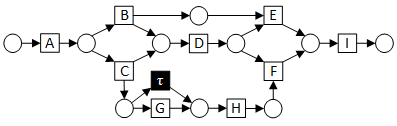
Figure 5: The ideal model. Fitting, fairly precise and properly generalizing.

Figure 6: Most frequent trace. Precise, but not fitting or generalizing.

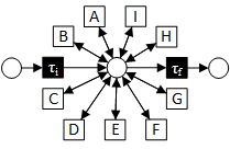
Figure 7: The flower model. Fitting and generalizing, but very imprecise.

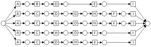
Figure 8: All traces separate. Fitting, precise, but not generalizing.

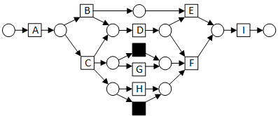
Figure 9: A model with G and H in parallel.

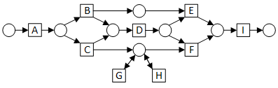
Figure 10: A model with G and H in self-loops

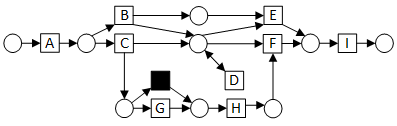
Figure 11: A model with D in a self-loop

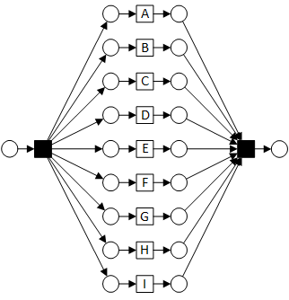
Figure 12: A model with all transitions in parallel.

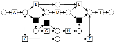
Figure 13: A model where C and F are in a loop, but need to be executed equally often to reach the final marking.

Figure 14: Round-robin model. The outer loop can be started at any point and then exited one transition before completing the loop.

A set of examples are taken from page 64 of [23], and consist of the simple event log shown in Table 1 aligned with 10 different process models. The log consists of only five different traces, with various frequencies. The models in Figures 5 to 8 are four examples of models often used to show the differences between fitness, precision and generalization. The model in Figure 5 shows the “ideal” process discovery result, i.e. the model that is fitting, fairly precise and properly generalizing. The models in Figures 9 to 12 present the same set of activities with varying loop and/or parallel constructs. Two new process models that describe particularly different routing logic from the previous models are depicted in Figures 13 and 14.

Model		$P_{ET}$	$P_{ETC}$	$P_{a}$	$P_{ne}$	$MAP^{3}$	$MAP^{7}$	$P^{H}_{aa}$	$P^{L}_{aa}$
Fig. 5	Generating model	0.992	0.994	0.982	0.995	0.880	0.852	0.818	0.955
Fig. 6	Single trace	1.000	1.000	1.000	0.893	1.000	1.000	1.000	1.000
Fig. 7	Flower model	0.136	0.119	0.142	0.117	0.003	0.000	0.181	0.364
Fig. 8	Separate traces	1.000	0.359	1.000	0.985	1.000	1.000	1.000	1.000
Fig. 9	G,H in parallel	0.894	0.936	0.947	0.950	0.564	0.535	0.818	0.955
Fig. 10	G,H as self-loops	0.884	0.889	0.947	0,874	0.185	0.006	0.272	0.727
Fig. 11	D as self-loop	0.763	0.760	0.797	0.720	0.349	0.069	0.272	0.727
Fig. 12	All parallel	0.273	0.170	0.336	0.158	0.006	0.000	0.181	0.500
Fig. 13	C,F equal loop	0.820	0.589	0.839	0.600	–	–	0.818	0.910
Fig. 14	Round-robin	0.579	0.185	0.889	0.194	0.496	0.274	0.181	0.636

Table 2: Precision measures for all models

Model		Hamming distance Anti-alignments	Edit distance Anti-alignments
Fig. 5	Generating model	$\langle A,C,G,H,D,F,I\rangle$	$\langle A,C,G,H,D,F,I\rangle$
Fig. 6	Single trace	$\langle A,B,D,E,I\rangle$	$\langle A,B,D,E,I\rangle$
Fig. 7	Flower model	$\langle tau,D,I,C,C,E,C,F,D,I,tau\rangle$	$\langle tau,G,G,G,G,G,G,G,G,G,tau\rangle$
Fig. 8	Separate traces	$\langle A,C,G,D,H,F,I\rangle$	$\langle A,C,D,H,F,I\rangle$
Fig. 9	G,H in parallel	$\langle A,C,D,H,G,F,I\rangle$	$\langle A,C,tau,tau,D,F,I\rangle$
Fig. 10	G,H as self-loops	$\langle A,C,H,H,D,G,G,G,G,F,I\rangle$	$\langle A,C,G,G,G,G,G,D,G,F,I\rangle$
Fig. 11	D as self-loop	$\langle A,C,D,D,D,D,G,H,D,F,I\rangle$	$\langle A,B,D,D,D,D,D,D,D,E,I\rangle$
Fig. 12	All parallel	$\langle tau,F,B,I,E,G,A,D,C,H,tau\rangle$	$\langle tau,I,E,D,B,C,F,A,H,G,tau\rangle$
Fig. 13	C,F equal loop	$\langle A,C,B,D,E,I\rangle$	$\langle A,C,B,D,E,F,I\rangle$
Fig. 14	Round-robin	$\langle tau,I,A,B,C,D,E,F,G,H,tau\rangle$	$\langle tau,E,F,G,H,I,A,B,C,D,tau\rangle$

Table 3: Anti-alignments of maximal size 11 for all models : interestingly, in some cases the Hamming anti-alingments are equal or very similar to the Levenshtein ones, which validates the use of the former (whose SAT encoding is simpler) as alternative for the latter. Also notice that in some cases, the fact that we require in this qualitative comparison to deal with full runs implies very different anti-alignments are obtained through the two distances (e.g., Figure 12).

Table 2 compares some precision metrics for the models in Figures 5 to 14 with the two possible metrics proposed in this paper: $P^{H}_{aa}$ and $P^{L}_{aa}$, representing the precision for the Hamming and Levenshtein distance, respectively. To understand the values provided by our proposed metrics, the reader can find in Table 3 the anti-alignments computed for each process model, both for the Hamming and the Levenshtein distances. Observe that, as a consequence of Lemma 1, $P^{H}_{aa}\leq P^{L}_{aa}$ for all models. The values of $P_{a}$ are defined as in [1]. The precision values in $P_{ET}$ and $P_{ETC}$ are defined in [2]. The value $P_{ne}$ denotes the precision metric from [32]. Finally, the values $MAP^{3}$ and $MAP^{7}$ are defined in [4]; because they rely on behavioral abstractions which are based on refinements of the directly-follows graph [18], they can dramatically overestimate the behavior of the model, therefore they tend to be pessimistic. For instance, for well chosen values of $k$, $MAP^{k}$ would use the same abstraction for two models $N_{1}$ and $N_{2}$ having languages $\mathcal{L}(N_{1})=a^{*}b^{3}c^{*}|d^{*}b^{3}e^{*}$ and $\mathcal{L}(N_{2})=(a^{*}|d^{*})b^{3}(c^{*}|e^{*})$ and assign them the same precision. Intuitively, this is not satisfactory: assume that the log contains only traces in $\mathcal{L}(N_{1})$, then model $N_{1}$ should score much better than $N_{2}$.

Clearly, the existing precision metrics do not agree on all models and do not always agree with the intuition for precision. For example, the very precise model of Figure 8 is considered to have a precision of $0.359$ by the $P_{ETC}$ metric. Also, the model of Figure 10 scores very high in $P_{ET}$-$P_{ETC}$-$P_{a}$, although a trace with a thousand G’s is possible in the model. Our metric $P^{L}_{aa}$ for this model however cannot fully penalize this, due to the requirement to deal with full run anti-alignments (see the anti-alignment in Table 3, which only differs with the log in the infix part). However, if we allowed for a larger run, e.g., doubling the length of the anti-alignment ($22$), the value would drop from $P^{L}_{aa}=0.727$ to $P^{L}_{aa}=0.613$ . A similar situation, with the same antidote, happens with the flower model, i.e., the value obtained for the Levenshtein based anti-alignment is higher than the rest, due to requiring the $\tau$ transitions that do not penalize in terms of distance.

7.3 Quantitative Comparison

In this section, we evaluate the techniques of this paper for 12 available real-life logs of varying sizes, and which have been recently used for benchmarking process discovery methods [6]. They cover different fields, ranging from finance through to healthcare and government. The logs are publicly available at the 4DTU Data Center. The experiments have been executed on a virtual machine with Debian 3.16.43-2+deb8u2 system, 12 CPU Intel Xeon 2.67GHz and 50GB RAM.

7.3.1 Benchmark Description

For each of the twelve logs, we compute precision for the models automatically discovered with two state-of-the-art discovery algorithms: Inductive Miner [18], and Split Miner [5]. We compare the performance of computing our metric against the one required for the $MAP$ metric [4], which is known to be the most recent precision contribution. Given that both methods are known to incur into a high complexity (specially in terms of memory footprint), we use samples of size 10 and 100 of the initial log. Similarly to [4], we present average execution times of precision computations of the twelve models and the samples. This is enough to get an insight on the empirical positioning of our approach with respect to the aforementioned work. Since the compared techniques strongly depend on models sizes, that vary between 8 to 150 transitions, we also report the minimal and maximum time performance of each method.

The notation $P_{aa_{10}}$ in Tab. 4 indicates that we use the simpler prefix variant of anti-alignments (see Section 7.1). As explained in Section  7.1, a second parameter, $max\_d$, helps to reduce complexity of the SAT formula by bounding the number of maximal differences: in all but the last row, we use $max\_d=20$. In the last row we set $max\_d$ to $10$, due to the computational requirements of that last set of benchmarks.

In this section, we compare our work against $MAP$ with $k=3$ as advised by the authors.

7.3.2 Discussion

By relying on approximations of anti-alignments (with prefixes instead of full runs, but also by limiting the maximal number of differences), our approach tends to run in reasonable time. We compare our method to $MAP^{3}$ which has shown good performances in [4]. For some models and logs, for instance model of BPI’2015 discovered with inductive miner and a log of size 10, we obtain better execution times for both Hamming and Levenshtein based precision. More generally Tab. 4 shows that Hamming based precision, which gives an approximation of Levenshtein based precision, is often the quicker approach. We see that for the first time, our tool can deal reasonably with large problem instances, when it is compared to the previous implementations. It should be stressed that several engineering efforts can be incorporated into the current tool, to drastically reduce part of its computational demands.

$|L|$	Method	Inductive Miner			Split Miner
		avg	min	max	avg	min	max
10	$MAP^{3}$	102.314	0.519	896.299	0.577	0.439	0.823
	$P_{aa_{10}}^{H}$	6.981	0.903	17.843	6.154	1.078	14.707
	$P_{aa_{10}}^{L}$	121.95	19.201	246.876	102.103	28.574	189.876
100	$MAP^{3}$	111.219	0.612	889.024	0.759	0.526	1.129
	$P_{aa_{10}}^{H}$	16.92	7.779	30.492	15.544	8.278	27.059
	$\sim P_{aa_{10}}^{L}$	632.519	99.269	1229.862	499.762	138.501	921.791

Table 4: Execution Times (in seconds) using the twelve real-life logs obtained on a virtual machine with CPU Intel Xeon 2.67GHz and 50GB RAM.

8 Related Work

The seminal work in [24] was the first one in relating observed behavior (in form of a set of traces), and a process model. In order to asses how far can the model deviate from the log, the follows and precedes relations for both model and log are computed, storing for each relation whereas it always holds or only sometimes. In case of the former, it means that there is more variability. Then, log and model follows/precedes matrices are compared, and in those matrix cells where the model has a sometimes relation whilst the log has an always relation indicate that the model allows for more behavior, i.e., a lack of precision. This technique has important drawbacks: first, it is not general since in the presence of loops in the model the characterization of the relations is not accurate [24]. Second, the method requires a full state-space exploration of the model in order to compute the relations, a stringent limitation for models with large or even infinite state spaces.

In order to overcome the limitations of the aforementioned technique, a different approach was proposed in [20]. The idea is to find escaping arcs, denoting those situations where the model starts to deviate from the log behavior, i.e., events allowed by the model not observed in the corresponding trace in the log. The exploration of escaping arcs is restricted by the log behavior, and hence the complexity of the method is always bounded. By counting how many escaping arcs a pair (model, log) has, one can estimate the precision of a model. Although being a sound estimation for the precision metric, it may hide the problems we are considering in this paper, i.e., models containing escaping arcs that lead to a large behavior.

Less related is the work in [32], where the introduction of weighted artificial negative events from a log is proposed. Given a log $L$, an artificial negative event is a trace $\sigma^{\prime}=\sigma\cdot a$ where $\sigma\in L$, but $\sigma^{\prime}\notin L$. Algorithms are proposed to weight the confidence of an artificial negative event, and they can be used to estimate the precision and generalization of a process model [32]. Like in [20], by only considering one step ahead of log/model’s behavior, this technique may not catch serious precision/generalization problems.

Finally, an automata-based technique is presented in [19]. The technique projects event log and process model onto all subsets of activities of size $k$, and generates minimal deterministic finite automata that conjunctively represents both perspectives, so that precision can be estimated by confronting the model and the conjunction automata.

As we mentioned in Section 6.2, a recent study elaborated on the guarantees provided by the aforementioned precision metrics [26]. The study shows that none of the precision metrics up to that moment (including an earlier version of the metrics described in this paper [30]) was able to satisfy all the properties together. Recently, however, a metric was proposed in [4] which satisfies the 5 axioms. Likewise to the metric in [4], the new precision metric proposed in this paper is shown to satisfy either these properties, or a weaker version of them.

9 Conclusions and Future Work

Conformance checking is becoming an important tool to certify the correct execution of processes in organizations. Quality metrics for conformance checking are crucial to evaluate quantitatively process models, and among the four dimensions to attain this task, precision is an important one. This paper proposes anti-alignments as a crucial artefact to compute an accurate metric for precision. In contrast to existing metrics, anti-alignment based precision metrics satisfy most of the properties for precision described in [26].

As future work, we plan to explore new algorithms to compute anti-alignments so that the complexity of the problem can be alleviated in practice. Also, we will consider new areas for the application of anti-alignments, like process model comparison or novel ways of computing the generalization of process models (we already suggested one such approach in a recent paper [30]).

We see potential for other notions of anti-alignments, for instance anti-alignments can be generalized between two nets: to find behavior of the former that cannot be found in the latter. The application of this generalization goes beyond the field of process mining: it can be used, for instance, to allow generating behavior that is not possible in a model, by simply aligning the net that allows for all the possible behaviors with the original net. This way, one can compute the most deviating trace of a net with respect to its own behavior, up to a given length. A second application of anti-alignments between two nets is for assessing behavioral process model similarity: this way, example behavior that is in one model and not in the other can be provided as a hint on the dissimilarity between two models. Previous techniques focus on the differences on either the causal relations, or those parts of the models that are different [3, 13, 22, 34, 35].

Acknowledgments.

This work has been partially supported by funds from ENS Paris-Saclay (project ProMAut of the Farman institute), the Spanish Ministry for Economy and Competitiveness (MINECO) and the European Union (FEDER funds) under grant GRAMM (TIN2017-86727-C2-1-R).

References

- [1] Arya Adriansyah. Aligning observed and modeled behavior. PhD thesis, Technische Universiteit Eindhoven, 2014.
- [2] Arya Adriansyah, Jorge Munoz-Gama, Josep Carmona, Boudewijn F. van Dongen, and Wil M. P. van der Aalst. Measuring precision of modeled behavior. Inf. Syst. E-Business Management, 13(1):37–67, 2015.
- [3] Abel Armas-Cervantes, Paolo Baldan, Dumas Marlon, and Luciano García-Bañuelos. Behavioral comparison of process models based on canonically reduced event structures. Business Process Management: 12th International Conference, BPM 2014, Haifa, Israel, September 7-11, 2014. Proceedings, pages 267–282, 2014.
- [4] Adriano Augusto, Abel Armas-Cervantes, Raffaele Conforti, Marlon Dumas, Marcello La Rosa, and Daniel Reißner. Abstract-and-compare: A family of scalable precision measures for automated process discovery. In Business Process Management - 16th International Conference, BPM 2018, Sydney, NSW, Australia, September 9-14, 2018, Proceedings, pages 158–175, 2018.
- [5] Adriano Augusto, Raffaele Conforti, Marlon Dumas, and Marcello La Rosa. Split miner: Discovering accurate and simple business process models from event logs. In 2017 IEEE International Conference on Data Mining (ICDM), pages 1–10. IEEE, 2017.
- [6] Adriano Augusto, Raffaele Conforti, Marlon Dumas, Marcello La Rosa, Fabrizio Maria Maggi, Andrea Marrella, Massimo Mecella, and Allar Soo. Automated discovery of process models from event logs: Review and benchmark. IEEE Trans. Knowl. Data Eng., 31(4):686–705, 2019.
- [7] Alessandro Berti, Sebastiaan J van Zelst, and Wil van der Aalst. Process Mining for Python (PM4Py): Bridging the Gap Between Process-and Data Science. page 13–16, 2019.
- [8] Joos C. A. M. Buijs, Boudewijn F. van Dongen, and Wil M. P. van der Aalst. Quality dimensions in process discovery: The importance of fitness, precision, generalization and simplicity. Int. J. Cooperative Inf. Syst., 23(1), 2014.
- [9] Josep Carmona, Boudewijn F. van Dongen, Andreas Solti, and Matthias Weidlich. Conformance Checking - Relating Processes and Models. Springer, 2018.
- [10] Thomas Chatain and Josep Carmona. Anti-alignments in conformance checking - the dark side of process models. In Application and Theory of Petri Nets and Concurrency - 37th International Conference, PETRI NETS 2016, Toruń, Poland, June 19-24, 2016. Proceedings, pages 240–258, 2016.
- [11] Allan Cheng, Javier Esparza, and Jens Palsberg. Complexity results for 1-safe nets. Theor. Comput. Sci., 147(1&2):117–136, 1995.
- [12] Wojciech Czerwinski, Slawomir Lasota, Ranko Lazic, Jérôme Leroux, and Filip Mazowiecki. The reachability problem for petri nets is not elementary. In Proceedings of the 51st Annual ACM SIGACT Symposium on Theory of Computing, STOC 2019, pages 24–33. ACM, 2019.
- [13] Remco M. Dijkman. Diagnosing differences between business process models. In BPM 2008, Milan, Italy, September 2-4, pages 261–277, 2008.
- [14] Niklas Eén and Niklas Sörensson. An extensible sat-solver. In Theory and Applications of Satisfiability Testing, 6th International Conference, SAT 2003. Santa Margherita Ligure, Italy, May 5-8, 2003 Selected Revised Papers, pages 502–518, 2003.
- [15] Alexey Ignatiev, Antonio Morgado, and Joao Marques-Silva. Rc2: a python-based maxsat solver. MaxSAT Evaluation 2018, page 22.
- [16] Alexey Ignatiev, Antonio Morgado, and Joao Marques-Silva. PySAT: A Python toolkit for prototyping with SAT oracles. In SAT, pages 428–437, 2018.
- [17] Markus Krötzsch, Tomáš Masopust, and Michaël Thomazo. Complexity of universality and related problems for partially ordered NFAs. Information and Computation, 255:177 – 192, 2017.
- [18] Sander JJ Leemans, Dirk Fahland, and Wil MP van der Aalst. Discovering block-structured process models from event logs-a constructive approach. In International conference on applications and theory of Petri nets and concurrency, pages 311–329. Springer, 2013.
- [19] S.J.J. Leemans, D. Fahland, and W.M.P. van der Aalst. Scalable process discovery and conformance checking. Software and Systems Modeling, pages 1–33, 2016.
- [20] Jorge Munoz-Gama. Conformance Checking and Diagnosis in Process Mining. PhD thesis, Universitat Politecnica de Catalunya, 2014.
- [21] T. Murata. Petri nets: Properties, analysis and applications. Proceedings of the IEEE, 77(4):541–574, April 1989.
- [22] Artem Polyvyanyy, Matthias Weidlich, Raffaele Conforti, Marcello La Rosa, and Arthur H. M. ter Hofstede. The 4c spectrum of fundamental behavioral relations for concurrent systems. In PETRI NETS 2014, Tunis, Tunisia, June 23-27, pages 210–232, 2014.
- [23] Anne Rozinat. Process Mining: Conformance and Extension. PhD thesis, Technische Universiteit Eindhoven, 2010.
- [24] Anne Rozinat and Wil M. P. van der Aalst. Conformance checking of processes based on monitoring real behavior. Inf. Syst., 33(1):64–95, 2008.
- [25] Iain A. Stewart. Reachability in some classes of acyclic Petri nets. Fundam. Inform., 23(1):91–100, 1995.
- [26] Niek Tax, Xixi Lu, Natalia Sidorova, Dirk Fahland, and Wil M.P. van der Aalst. The imprecisions of precision measures in process mining. Information Processing Letters, 135:1 – 8, 2018.
- [27] G. S. Tseytin. On the complexity of derivation in propositional calculus. In A.O. Slisenko, editor, Studies in Constructive Mathematics and Mathematical Logic, Part II, Seminars in Mathematics, page 115–125. Steklov Mathematical Institute, 1970. Translated from Russian: Zapiski Nauchnykh Seminarov LOMI 8 (1968), pp. 234–259.
- [28] Wil M. P. van der Aalst. Process Mining - Data Science in Action, Second Edition. Springer, 2016.
- [29] Wil M. P. van der Aalst, Anna Kalenkova, Vladimir Rubin, and Eric Verbeek. Process discovery using localized events. In Application and Theory of Petri Nets and Concurrency - 36th International Conference, PETRI NETS 2015, Brussels, Belgium, June 21-26, 2015, Proceedings, pages 287–308, 2015.
- [30] Boudewijn F. van Dongen, Josep Carmona, and Thomas Chatain. A unified approach for measuring precision and generalization based on anti-alignments. In Business Process Management - 14th International Conference, BPM 2016, Rio de Janeiro, Brazil, September 18-22, 2016. Proceedings, pages 39–56, 2016.
- [31] Seppe K. L. M. vanden Broucke, Jorge Munoz-Gama, Josep Carmona, Bart Baesens, and Jan Vanthienen. Event-based real-time decomposed conformance analysis. In On the Move to Meaningful Internet Systems: OTM 2014 Conferences - Confederated International Conferences: CoopIS, and ODBASE 2014, Amantea, Italy, October 27-31, 2014, Proceedings, pages 345–363, 2014.
- [32] Seppe K. L. M. vanden Broucke, Jochen De Weerdt, Jan Vanthienen, and Bart Baesens. Determining process model precision and generalization with weighted artificial negative events. IEEE Trans. Knowl. Data Eng., 26(8):1877–1889, 2014.
- [33] HMW Verbeek, JCAM Buijs, BF Van Dongen, and Wil MP van der Aalst. Prom 6: The process mining toolkit. Proc. of BPM Demonstration Track, 615:34–39, 2010.
- [34] Matthias Weidlich, Jan Mendling, and Mathias Weske. Efficient consistency measurement based on behavioral profiles of process models. IEEE Tr. Soft. Eng., 37(3):410–429, 2011.
- [35] Matthias Weidlich, Artem Polyvyanyy, Jan Mendling, and Mathias Weske. Causal behavioural profiles - efficient computation, applications, and evaluation. Fundam. Inform., 113(3-4):399–435, 2011.
- [36] H. Yang, B. F. van Dongen, A. H. M. her Hofstede, M. T. Wynn, and J. Wang. Estimating completeness of event logs. Technical Report BPM-12-04, BPM Center, 2012.