Variational Coupling Revisited: Simpler Models, Theoretical Connections, and Novel Applications

Abstract

Variational models with coupling terms are becoming increasingly popular in image analysis. They involve auxiliary variables, such that their energy minimisation splits into multiple fractional steps that can be solved easier and more efficiently. In our paper we show that coupling models offer a number of interesting properties that go far beyond their obvious numerical benefits.
We demonstrate that discontinuity-preserving denoising can be achieved even with quadratic data and smoothness terms, provided that the coupling term involves the $L^{1}$ norm. We show that such an $L^{1}$ coupling term provides additional information as a powerful edge detector that has remained unexplored so far.
While coupling models in the literature approximate higher orderregularisation, we argue that already first order coupling models can be useful. As a specific example, we present a first order coupling model that outperforms classical TV regularisation. It also establishes a theoretical connection between TV regularisation and the Mumford-Shah segmentation approach. Unlike other Mumford-Shah algorithms, it is a strictly convex approximation, for which we can guarantee convergence of a split Bregman algorithm.

Aaron Wewior and Joachim Weickert

Mathematical Image Analysis Group,

Faculty of Mathematics and Computer Science, Campus E1.7, Saarland University

66041 Saarbrücken, Germany

1 Introduction

In image analysis applications, it is desirable to use variational models with regularisers that involve higher order derivatives: These higher order models offer better smoothness and avoid e.g. staircasing artifacts that are present in various first order variational approaches. Unfortunately, higher order variational models are numerically unpleasant. For instance, minimising a second order energy gives rise to a fourth order partial differential equation (PDE) as Euler-Lagrange equation. Higher order PDEs are more cumbersome to discretise, and their numerical approximations suffer from higher condition numbers such that algorithms converge more slowly or become even unstable.

As a remedy, coupling models have been proposed. They introduce coupling terms with auxiliary variables. For instance, one approximates the gradient of the processed image by an auxiliary variable. In this way a second order energy in a single variable is replaced by a first order energy in two variables. As Euler-Lagrange equations, one solves a system of second order PDEs, which is numerically more pleasant than solving a fourth order PDE.

Coupling models have a long history. Already in 1990, Horn came up with a coupling model for shape from shading [19]. In the case of denoising and deblurring, Chambolle and Lions [13] have investigated coupling models by combining several convex functionals into one regulariser. With this they were able to modify the total variation regularisation model [24] and reduce unpleasant staircasing artifacts. A transfer of this infimal convolution approach to the discrete setting was proposed by Setzer et al. [27]. Also Bredies et al. [7] performed research in this direction and introduced a total generalised variation regulariser based on symmetric tensors of varying order. This allows a selective regularisation with different smoothness constraints. More recent coupling models have become highly sophisticated. Hewer et al. [18] introduced three coupling variables to come up with a coupling model that replaces fourth order energy minimisation. Hafner et al. [17] considered coupling models that are anisotropic both in the coupling and the smoothness term, and Brinkmann et al. [8] used coupling models in connection with regularisers based on natural vector field operations, including divergence and curl terms.

Nevertheless, in spite of their popularity and sophistication, the main motivation behind all these coupling approaches was numerical efficiency. Additional benefits of the coupling formulation have hardly been investigated so far.

Our Contributions. The goal of our paper is to show that the coupling formulation is much more than just a numerical acceleration strategy. We will see that it provides valuable benefits from three different perspectives that have remained unexplored so far:

• From a modelling perspective, we argue that coupling terms may free the user from designing nonquadratic smoothness terms if discontinuity-preserving solutions are needed. Moreover, we show that it can be worthwhile to replace even first order energies by coupling models.

• From a theoretical perspective, we demonstrate that coupling models may give insights into the connections between two of the most widely used variational approaches in image analysis: the total variation (TV) regularisation of Rudin et al. [24] and the Mumford-Shah functional [22] for image segmentation. These insights will also give rise to a new algorithm for Mumford-Shah segmentation, that differs from existing ones by the fact that it minimises a strictly convex energy. Thus, we can guarantee convergence of a split Bregman algorithm.

• From an application perspective, we show that sparsity promoting coupling terms may provide useful information as an edge detector that comes at no additional cost.

Paper Structure. Our paper is organised as follows: In Section 2, we derive the framework for a first and second order model that incorporates the coupling term. We show the relation to the Mumford-Shah functional and elaborate why the coupling term can be interpreted as an edge detector. Section 3 deals with the numerical aspects that lead to the minimisation of our approach in the discrete setting and showcases the advantages of the split Bregman formulation. In Section 4, we present experimental results, and we conclude the paper in Section 5.

2 Our Models

In this section we propose two coupling models for edge-preserving image enhancement. We relate them to total variation regularisation and the segmentation approach of Mumford and Shah, and we argue that the $L^{1}$ coupling term provides a novel edge detector.

2.1 Coupling Framework

2.1.1 First Order Model.

Let our image domain $\Omega\subset\mathbb{R}^{2}$ be an open bounded set and $f:\Omega\to\mathbb{R}$ denote a greyscale image that contains noise with zero mean. Our goal is to find a noise free version of that image. As this is in general an ill-posed problem, we employ variational approaches to find a reconstruction $u$ that is as close as possible to the noise free image and at the same time satisfies certain a priori smoothness conditions. One of the earliest models by Whittaker [29] and Tikhonov [28] obtains $u$ as minimiser of the energy functional

$$E(u)=\int_{\Omega}\left(\frac{1}{2}(u-f)^{2}+\frac{\alpha}{2}\|\bm{\nabla}u\|^{2}\right)\text{ d}{\bm{x}}\,,$$ (1)

where $\|\cdot\|$ denotes the Euclidian norm. The first term guarantees that $u$ is close to the given data $f$ and is called data term. The second term penalises deviation from a smooth solution and is therefore denoted as the smoothness term. The regularisation parameter $\alpha>0$ steers the smoothness of the solution. In practice we deal with a rectangular, finite domain $\Omega$. This prompts us to choose homogeneous Neumann boundary conditions. These coincide with the natural boundary conditions that arise when we derive the Euler-Lagrange equations of (1).

We modify (1) to a constrained problem by introducing an auxiliary vector field $\bm{v}\in L^{2}(\Omega,\mathbb{R}^{2})$. We set $\bm{v}=\bm{\nabla}u$ and obtain

$$E(u)=\int_{\Omega}\left(\frac{1}{2}(u-f)^{2}+\frac{\alpha}{2}\|\bm{v}\|^{2}\right)\text{ d}{\bm{x}}\qquad\text{ s.t. }\bm{v}=\bm{\nabla}u\,.$$ (2)

Enforcing the constraint weakly in the Euclidian norm yields the coupling model

$$E(u,\bm{v})=\int_{\Omega}\left(\frac{1}{2}(u-f)^{2}+\frac{\alpha}{2}\|\bm{v}\|^{2}+\frac{\beta}{2}\|\bm{\nabla}u-\bm{v}\|^{2}\right)\text{ d}{\bm{x}}$$ (3)

with parameter $\beta>0$. Since the newly introduced term inherently couples $\bm{\nabla}u$ and $\bm{v}$ we call it coupling term. It is obvious that apart from trivial cases the vector field $\bm{v}$ is not equal to the gradient of the function $u$. However, by following the proof in [4] one can show that

$$\int_{\Omega}\bm{v}\text{ d}{\bm{x}}=\int_{\Omega}\bm{\nabla}u\text{ d}{\bm{x}}\,,$$ (4)

which means that they are ”equal in the mean”. The vector field $\bm{v}$ inherits its boundary conditions from $u$. We will discuss the details in the next chapter.

At first sight the coupling model does not offer any advantage over the energy (1) and seems to complicate it more. Indeed, by calculating the Euler-Lagrange equations and performing a simple substitution we see that the minimiser for $u$ of the functional in (3) is equivalent to the minimiser of energy (1) with parameter $\frac{\alpha\beta}{\alpha+\beta}$. For the limit case $\beta\rightarrow\infty$, which corresponds to a hard constraint of $\bm{\nabla}u=\bm{v}$, we thus obtain the same solution. In the other limit case $\alpha\rightarrow\infty$, the energy (3) corresponds to (1) with regularisation parameter $\beta$.

In order to obtain our first order coupling model we only apply a small modification to the coupling term in (3). We recall that a function $u\in{L}^{1}(\Omega)$ is said to be of bounded variation ($u\in BV(\Omega)$) if it has a (distributional) gradient in form of a Radon measure of finite total mass. Then we can define the total variation seminorm of $u$ as [2]

$$\int_{\Omega}|\bm{\nabla}u|:=\sup\left\{\int_{\Omega}u\,\text{div}\bm{\phi}\text{ d}{\bm{x}}\,|\,\bm{\phi}\in\mathcal{C}^{1}_{c}(\Omega,\mathbb{R}^{2}),\,|\bm{\phi}|<1\right\}.$$ (5)

If we consider the difference $\bm{\nabla}u-\bm{v}$ as an argument, we extend (5) and obtain

$$\int_{\Omega}|\bm{\nabla}u-\bm{v}|:=\sup\left\{\int_{\Omega}u\,\text{div}\bm{\phi}+\bm{v}^{\top}\bm{\phi}\text{ d}{\bm{x}}\,|\,\bm{\phi}\in\mathcal{C}^{1}_{c}(\Omega,\mathbb{R}^{2}),\,|\bm{\phi}|<1\right\}.$$ (6)

With this we formulate our first order coupling model:

$$\boxed{E_{1}(u,{\bm{v}}):=\frac{1}{2}\int_{\Omega}(u-f)^{2}\text{ d}{\bm{x}}+\frac{\alpha}{2}\int_{\Omega}\|{\bm{v}}\|^{2}\text{ d}{\bm{x}}+\beta\int_{\Omega}|{\bm{\nabla}}u-{\bm{v}}|\,.}$$ (7)

It is obvious that the model (7) is strictly convex due to the quadratic data term. Moreover, we also have a quadratic smoothness term and only the coupling term contains a more sophisticated penaliser. It is therefore no surprise that for the hard constraint $\beta\rightarrow\infty$, the energies (7) and (3) are still identical. The more interesting case arises in the limit $\alpha\rightarrow\infty$: In order to fulfil the constraint, the vector field $\bm{v}$ should be zero, which yields the regulariser (5) for the coupling term. Energy (7) is then equivalent to the classical TV denoising model by Rudin et al. [24]. However, we will later demonstrate how the structure of the coupling model is both beneficial for an efficient minimisation as well as for superior denoising results. We note that it can be shown that model (7) is equivalent to denoising with a Huber TV penaliser [10].

2.1.2 Second Order Model.

While TV regularisation promises a good compromise between image reconstruction and edge preservation, it introduces ”blocky” structures into the reconstructed images, the so-called staircasing artifacts. One way to avoid these artifacts is by second order models [25, 30, 21]. Due to the coupling formulation, a higher regularisation order can easily be realised in our framework. Instead of the vector field $\bm{v}$ we penalise its Jacobi matrix in the Frobenius norm. The resulting energy is given by

$$\boxed{E_{2}(u,{\bm{v}}):=\frac{1}{2}\int_{\Omega}(u-f)^{2}\text{ d}{\bm{x}}+\frac{\alpha}{2}\int_{\Omega}\|{\bm{\nabla}\bm{v}}\|_{F}^{2}\text{ d}{\bm{x}}+\beta\int_{\Omega}|{\bm{\nabla}}u-{\bm{v}}|\,.}$$ (8)

In order to see that (8) approximates a second order model, we discuss the limiting case $\beta\rightarrow\infty$ again. The smoothness term favours a constant vector field $\bm{v}$. For a hard coupling this means that constant first derivatives of $u$ lead to the smallest energy. Hence, the solution $u$ corresponds to an affine function which is characteristic for second order regularisation methods. The model resembles the total generalized variation (TGV) of second order [7]:

$$E_{TGV}(u,{\bm{v}}):=\frac{1}{2}\int_{\Omega}(u-f)^{2}\text{ d}{\bm{x}}+\alpha\int_{\Omega}|{\bm{\varepsilon}(\bm{v})}|+\beta\int_{\Omega}|{\bm{\nabla}}u-{\bm{v}}|$$ (9)

where $\bm{\varepsilon}$ denotes the symmetrised gradient in a TV-like norm in the smoothness term. However, the smoothness term in our first and second order model is still quadratic. In Section 3 we will see that this allows very efficient algorithms.

2.2 Relation to the Segmentation Model of Mumford and Shah

Let $\Omega$ be defined as before and let $K$ be a compact curve in $\Omega$. The segmentation model by Mumford and Shah minimises the following energy [22]:

$$E_{MS}(u,K)=\frac{1}{2}\int_{\Omega}(u-f)^{2}\text{ d}{\bm{x}}+\frac{\alpha}{2}\int_{\Omega\backslash K}\|\bm{\nabla}u\|^{2}\text{ d}{\bm{x}}+\beta\,\ell(K)\,.$$ (10)

The function $u:\Omega\rightarrow\mathbb{R}$ approximates $f$ as a sufficiently smooth function in $\Omega\backslash K$, but admits discontinuities across $K$. The curve $K$ denotes the edge set between the segments. The expression $\ell(K)$ represents the length of $K$ and can be expressed as $\mathcal{H}^{1}(K)$, the one-dimensional Hausdorff measure in $\mathbb{R}^{2}$. The parameter $\beta>0$ controls the length of the edge set, whereas $\alpha>0$ steers the smoothness of $u$ in $\Omega\backslash K$.

Unfortunately the Mumford-Shah energy is highly non-convex and difficult to minimise. Ambrosio and Tortorelli [3] showed that they can approximate the solution by a sequence of regular functions defined on Sobolev spaces and proved $\Gamma$-convergence. However, their energy is still non-convex and the quality of the solution depends on the initial parameter setting of the $\epsilon$-approximation.

Cai et al. [11] proposed a variant that approximates the edge length by the total variation seminorm. They were able to approximate (10) by a convex minimisation problem over the whole domain:

$$E_{\text{Cai}}(u)=\frac{1}{2}\int_{\Omega}(u-f)^{2}\text{ d}{\bm{x}}+\frac{\alpha}{2}\int_{\Omega}\|\bm{\nabla}u\|^{2}\text{ d}{\bm{x}}+\beta\int_{\Omega}|\bm{\nabla}u|\,.$$ (11)

Nevertheless, the price for convexity comes with a smooth minimiser $u\in W^{1,2}(\Omega)$ that cannot contain any discontinuities such that a postprocessing step is necessary for a segmentation.

In order to relate equation (11) to our first order model (7), we perform the image decomposition $u=u_{1}+u_{2}$ such that the regularisers affect different parts of the image. These kind of approaches based on an infimal convolution were introduced by Chambolle and Lions in [13]. With this we obtain

$$E(u_{1},u_{2})=\frac{1}{2}\int_{\Omega}(u_{1}+u_{2}-f)^{2}\text{ d}{\bm{x}}+\frac{\alpha}{2}\int_{\Omega}\|\bm{\nabla}u_{1}\|^{2}\text{ d}{\bm{x}}+\beta\int_{\Omega}|\bm{\nabla}u_{2}|\,.$$ (12)

The decomposition lets us define the parts on different spaces. While $u_{1}\in W^{1,2}(\Omega)$, we have $u_{2}\in BV(\Omega)$. Thus, we admit jumps in $u$ which makes a postprocessing unnecessary. By introducing an auxiliary vector field $\bm{v}\in L^{2}(\Omega,\mathbb{R}^{2})$ which is designed to approximate $\bm{\nabla}u_{1}$, we consequently obtain for the argument of the last term:

$$\bm{\nabla}u_{2}=\bm{\nabla}u-\bm{\nabla}u_{1}\approx\bm{\nabla}u-\bm{v}\,.$$ (13)

Substituting this in (12) brings us back to the coupling model (7). Therefore, we observe that our first order coupling model approximates the Mumford-Shah segmentation model. It is obvious that this convex approximation is smoother then other variants as we do not perform an enhancement at edges. However, we still allow jumps in the regularised image. Moreover, we stress that the approximation is strictly convex and admits a unique solution.

The reasoning for the first order model can easily be transferred to the second order model. Energy (8) can thus be understood as an approximation to a second order Mumford-Shah model. One example for a second order approximation is the model of Blake and Zisserman [5]:

$$\begin{split}E_{BZ}(u,K_{0},K_{1})=\frac{1}{2}\int_{\Omega}(u-f)^{2}\text{ d}{\bm{x}}+\frac{\alpha}{2}\int_{\Omega\backslash(K_{0}\cup K_{1})}\|\bm{\nabla}^{2}u\|^{2}\text{ d}{\bm{x}}\\ +\beta\,\mathcal{H}^{1}(K_{0})+\gamma\,\mathcal{H}^{1}(K_{1})\,.\end{split}$$ (14)

Here, $\bm{\nabla}^{2}$ denotes the Hessian, and the Hausdorff measures on the curves $K_{0}$ and $K_{1}$ penalise not only the edge length between segments as before, but also the length of the curve that describes creases in the image. More recent variants were discussed in [9, 15]. They all have in common that they require the approach of Ambrosio-Torterelli to derive a minimiser. Our second order model gives an alternative that manages without the $\epsilon$-approximation.

2.3 Interpretation of the Coupling Term as an Edge Detector

In the previous subsection we established a connection between our coupling framework and the Mumford-Shah functional. The difficulty in the original formulation lies in the computation of the edge set $K$. We argue in the following how the edge set is related to the introduced coupling term which is directly accessible without additional effort.

We observe that the smoothness terms in energy (7) and (8) are quadratic. That means that on one hand $\bm{v}$ is still a smooth approximation to the $\bm{\nabla}u$. On the other hand the coupling term contains the sparsity-promoting $L^{1}$ norm. As a result, $\bm{v}$ deviates from $\bm{\nabla}u$ only at a small number of positions, which are represented as peaks in the energy of the coupling term. Since these peaks correspond to discontinuous jumps in the solution $u$, we see that the coupling term corresponds to the desired edge set and can naturally be utilised as an edge detector.

We distinguish two limiting cases. For $\beta\rightarrow\infty$ we end up with the hard constraint $\bm{\nabla}u=\bm{v}$ such that the coupling energy (6) evaluates to $0$. This makes sense, as the model simplifies to energy (1) again, and $u$ will be a smooth solution without jumps. For $\beta\rightarrow 0$, the functions $u$ and $\bm{v}$ are decoupled. A minimiser is reached when $u$ corresponds to the given image $f$ and $\bm{v}=\bm{0}$. Here the coupling term represents a simple gradient-based edge detector without a presmoothing. Such a detector is not reliable in the presence of high frequency oscillations and noise as it responds to many false edges.

In between these limiting cases, an increasing value for $\beta$ allows the coupling term to partition the image into more and more homogeneous regions, since this gives a smaller energy. Thus, on each scale $\beta$, we solve a convex variational model and obtain a unique solution. The coupling term serves as a novel edge detector that provides us with a globally optimal edge set. The discontinuity-preserving $L^{1}$ norm in the underlying model allows the coupling term to respond at edges, but makes it robust against false edges produced by noise in the image. As it also promotes sparsity it limits the detector’s response to the most relevant edges which are well localised.

3 Numerical Aspects

In this section we argue that the discrete variables in our models live on different grids in order to obtain consistent approximations. We speed up a conventional alternating minimisation by a split Bregman scheme [16] that offers a tremendous acceleration of the minimisation process. We discuss the scalar-valued problem and then explain the modification needed to solve the problem for vector-valued data.

3.1 Discretisation of the Variables

In order to implement the model on a computer we introduce a discrete setting based on a finite difference discretisation. We consider the domain $\Omega$ to be rectangular, i.e. $\Omega=(a,b)\times(c,d)$. Then the discrete domain $\Omega_{d}$ is given on a regular Cartesian grid with $M\times N$ nodes:

$$\Omega_{d}:=\left\{\left(a+\left(i-\tfrac{1}{2}\right)h,c+\left(j-\tfrac{1}{2}\right)h\right):1\leq i\leq M,\,1\leq j\leq N\right\}$$ (15)

with grid size $h:=\frac{b-a}{M}=\frac{d-c}{N}$. The discrete locations $(i,j)$ within $\Omega_{d}$ correspond w.l.o.g. to the continuous locations $\left(a+\left(i-\frac{1}{2}\right)h,\,c+\left(j-\frac{1}{2}\right)h\right)$ within $\Omega$. Discretising the scalar-valued functions $u$ and $f$ at positions $(i,j)$ yields variables $\bm{u},\bm{f}\in\mathbb{R}^{M\times N}$. We approximate the derivatives with a finite difference scheme. As we require the consistency order of our approximation to be at least two, we use central differences around a grid shifted by $\frac{h}{2}$. In order to be consistent with this approximation we consequently need the discretisation for $\bm{v}=({\bm{v}_{1}},{\bm{v}_{2}})^{\top}$ to live on different dual grids shifted just by this half grid size [20]. More precisely, entries $(v_{1})_{i,j}$ are defined at positions $(i+\frac{1}{2},j)$, whereas entries $(v_{2})_{i,j}$ are defined at positions $(i,j+\frac{1}{2})$, as they approximate the partial derivatives in different directions. This also extends to the boundary conditions. As already mentioned $\bm{v}$ inherits its boundary conditions from the homogeneous Neumann boundary conditions of $\bm{u}$. This means that the components of $\bm{v}$ have zero Dirichlet boundary conditions in the direction of the shifted grid and homogeneous Neumann boundary conditions otherwise.

3.2 Discretisation of the Energies

For sufficiently smooth data $u$, we can define a regularised penaliser of (5) by

$$\int\limits_{\Omega}\varphi_{\epsilon}(\bm{\nabla}u)\text{ d}{\bm{x}}=\int\limits_{\Omega}\sqrt{\|\bm{\nabla}u\|^{2}+\epsilon}\text{ d}{\bm{x}}$$ (16)

with small $\epsilon\geq 0$ [1]. For the case $\epsilon=0$, it reduces to (5), but otherwise offers the advantage to be differentiable when $\bm{\nabla}u=0$. We consider this regularisation for our discrete implementations.

The discretisation of our first order model (7) and second order model (8) subsume to the minimisation problem

$$\boxed{\min\limits_{\bm{u},\bm{v}}\left\{\frac{1}{2}\|\bm{u}-\bm{f}\|^{2}_{2}+\frac{\alpha}{2}\,S^{\ell}(\bm{v})+\beta\,C(\bm{\nabla}_{\!\!u}\bm{u}-\bm{v})\right\}}$$ (17)

where $\|\cdot\|_{2}$ denotes the discrete Euclidean norm. The coupling term contains the discrete counterpart of the regularised penalising function (16) in form of

$$C\left(\bm{\nabla}_{\!\!u}\bm{u}-\bm{v}\right)=\sum_{i=1}^{M}\sum_{j=1}^{N}\varphi_{\epsilon}(\|\bm{\nabla}_{\!\!u}\bm{u}-\bm{v}\|_{2}^{2})_{i,j}$$ (18)

which evaluates the regulariser (16) pixelwise with

$$\begin{split}\varphi_{\epsilon}(\|\bm{\nabla}_{\!\!u}\bm{u}{-}\bm{v}\|_{2}^{2})_{i,j}=\Bigg{(}\frac{1}{2}&\bigg{(}\left.(\partial_{x+}\bm{u}-v_{1})^{2}\right|_{i,j}+\left.(\partial_{x+}\bm{u}-v_{1})^{2}\right|_{i-1,j}\\[-10.76385pt] +&\left.(\partial_{y+}\bm{u}-v_{2})^{2}\right|_{i,j}+\left.(\partial_{y+}\bm{u}-v_{2})^{2}\right|_{i,j-1}\bigg{)}+\epsilon\Bigg{)}^{\frac{1}{2}}\!.\end{split}$$ (19)

The approximation of the discrete gradient components $\partial_{x+}\bm{u}$ and $\partial_{y+}\bm{u}$ lives on a grid shifted by half a grid size in the corresponding positive coordinate direction and incorporates the homogeneous Neumann boundary conditions.

In the function $S^{\ell}(\bm{v})$, the parameter $\ell$ defines the regularisation order of the problem. For $\ell=1$, we have $S^{1}(\bm{v})=\|\bm{v}\|^{2}_{2}$, and for $\ell=2$ we use $S^{2}(\bm{v})$ given by

$$\|\bm{\nabla}_{\!\!v}\bm{v}\|^{2}_{2}:=\sum_{i=1}^{M}\sum_{j=1}^{N}\left((\partial_{x-}\bm{v}_{1})^{2}_{i,j}+(\partial_{y+}\bm{v}_{1})^{2}_{i,j}+(\partial_{x+}\bm{v}_{2})^{2}_{i,j}+(\partial_{y-}\bm{v}_{2})^{2}_{i,j}\right)\,.$$ (20)

We employ the same discretisation for $\partial_{y+}\bm{v}_{1}$ and $\partial_{x+}\bm{v}_{2}$ as above, whereas we introduce the approximations $\partial_{x-}\bm{v}_{1}$ and $\partial_{y-}\bm{v}_{2}$ as central differences on a grid which is shifted in the respective negative coordinate with Dirichlet boundary conditions.

If we solve problem (17) in a naive way, we set the derivatives with respect to the components $\bm{u}$ and $\bm{v}$ to zero and perform an alternating iterative minimisation. The nonlinearity is always evaluated at the old iterate. The minimisation problem for $\bm{u}$ leads to

$$\bm{0}=\bm{u}-\bm{f}-\beta\textrm{ div}_{\!u}\left(\varphi_{\epsilon}^{\prime}(\|\bm{\nabla}_{\!\!u}\bm{u}^{k}-\bm{v}^{k}\|_{2}^{2})(\bm{\nabla}_{\!\!u}\bm{u}-\bm{v}^{k})\right)$$ (21)

with the diffusivity vector $\varphi_{\epsilon}^{\prime}(\|\bm{\nabla}_{\!\!u}\bm{u}^{k}-\bm{v}^{k}\|_{2}^{2})=\frac{1}{\sqrt{\|\bm{\nabla}_{\!\!u}\bm{u}^{k}-\bm{v}^{k}\|^{2}+\epsilon}}$ and a discrete divergence operator $\textrm{div}_{\!u}$. For $\ell=1$, the auxiliary vector field $\bm{v}$ requires us to solve the following equations:

$$\bm{0} =\varphi_{\epsilon}^{\prime}(\|\bm{\nabla}_{\!\!u}\bm{u}^{k}-\bm{v}^{k}\|_{2}^{2})(\bm{v}-\bm{\nabla}_{\!\!u}\bm{u}^{k+1})+\alpha\bm{v},$$ (22)

whereas for $\ell=2$ we obtain a system of equations of the form

$$\bm{0} =\varphi_{\epsilon}^{\prime}(\|\bm{\nabla}_{\!\!u}\bm{u}^{k}-\bm{v}^{k}\|_{2}^{2})(\bm{v}-\bm{\nabla}_{\!\!u}\bm{u}^{k+1})-\alpha\bm{\Delta}_{v}\bm{v}.$$ (23)

Here, $\bm{\Delta}_{v}$ denotes a direct sum of discrete Laplace operators that are applied to each component of $\bm{v}$ separately.

3.3 The Split Bregman Method

Unfortunately, the solution of (21) is a bottleneck in the alternating minimisation process. The derivatives of the regularised penalisation that serve as a diffusivity slow down the convergence speed drastically when we apply iterative solvers. As a remedy for this problem we employ the split Bregman method by Goldstein and Osher [16]. This operator splitting approach is equivalent to the alternating direction method of multipliers (ADMM) and the Douglas-Rachford splitting algorithm which are suitable for convex optimisation problems such as (17) and whose convergence is guaranteed [6, 26].

We introduce the discrete vector field $\bm{p}$ that lives on the same grid as $\bm{v}$. We set $\bm{p}:=\bm{\nabla}_{\!\!u}\bm{u}-\bm{v}$ and obtain the constrained problem

$$\min\limits_{\bm{u},\bm{v},\bm{p}}\left\{\frac{1}{2}\|\bm{u}-\bm{f}\|^{2}_{2}+\frac{\alpha}{2}\,S^{\ell}(\bm{v})+\beta\,C\left(\bm{p}\right)\right\}\quad\text{s.t. }\bm{p}=\bm{\nabla}_{\!\!u}\bm{u}-\bm{v}.$$ (24)

Enforcing the constraint strictly with a numerical parameter $\lambda>0$ yields the split Bregman iteration at step $k+1$:

$$\begin{split}(\bm{u}^{k+1},\bm{v}^{k+1},\bm{p}^{k+1})={}&\arg\min\limits_{\bm{u},\bm{v},\bm{p}}\left\{\frac{1}{2}\|\bm{u}-\bm{f}\|^{2}_{2}+\frac{\alpha}{2}\,S^{\ell}(\bm{v})+\beta\,C\left(\bm{p}\right)\right.\\ &\hskip 45.00006pt\left.+\,\frac{\lambda}{2}\|\bm{p}-\bm{\nabla}_{\!\!u}\bm{u}+\bm{v}-\bm{b}^{k}\|^{2}_{2}\right\},\end{split}$$ (25)

$$\bm{b}^{k+1}={} \bm{b}^{k}+\bm{\nabla}_{\!\!u}\bm{u}^{k+1}-\bm{v}^{k+1}-\bm{p}^{k+1}.$$ (26)

Even though the split Bregman method introduces an additional minimisation problem, the previous nonlinear equations are simplified substantially due to the simple quadratic structure of the data and smoothness term. The subproblems for $\bm{u}$ and $\bm{v}$ are then by design linear and yield the optimality conditions

$$\left(\bm{I}-\lambda\bm{\Delta}_{u}\right)\bm{u}\,\,=\,\, \bm{f}+\lambda\textrm{ div}_{\!u}\left(\bm{p}^{k}+\bm{v}^{k}-\bm{b}^{k}\right)\,,$$ (27)

$$\bm{v}\,\,=\,\, \frac{\lambda}{\alpha+\lambda}\left(\bm{\nabla}_{\!\!u}\bm{u}^{k+1}-\bm{p}^{k}+\bm{b}^{k}\right) \text{for }\ell=1,$$ (28)

$$\left(\lambda\bm{I}-\alpha\bm{\Delta}_{v}\right)\bm{v}\,\,=\,\, \lambda\left(\bm{\nabla}_{\!\!u}\bm{u}^{k+1}-\bm{p}^{k}+\bm{b}^{k}\right) \text{for }\ell=2.$$ (29)

Equation (28) leads to a simple pointwise computation. For the other two subproblems we may only apply a few steps of an iterative solver. This is in accordance to Osher and Goldstein who state that a complete convergence of the subproblems is not necessary for the convergence of the whole algorithm [16].

The last subproblem for $\bm{p}$ contains the nonlinearity, that now only occurs pointwise and not as a diffusivity in a divergence term. We obtain the update rule

$$\bm{p}^{k+1}=\frac{\lambda}{\lambda+\varphi_{\epsilon}^{\prime}(\|\bm{p}^{k}\|_{2}^{2})}\left(\bm{\nabla}_{\!\!u}\bm{u}^{k+1}-\bm{v}^{k+1}+\bm{b}^{k}\right).$$ (30)

We terminate the algorithm if the residuum of equations (21)–(23) in relation to an initial residuum gets smaller than a prescribed threshold. If we are also interested in the resulting edge set, we can obtain it without additional effort by evaluating $\|\bm{\nabla}_{\!\!u}\bm{u}-\bm{v}\|_{2}^{2}$.

3.4 Vector-valued Extension

An extension to vector-valued images is straightforward. The Euclidian norm in data and smoothness terms allows a separate calculation for each channel which opens up the possibility for a parallel implementation. The only coupling between channels occurs in (19). Therefore, only the nonlinearities in the pointwise update rule (30) are affected.

4 Experiments

4.1 Denoising Experiment

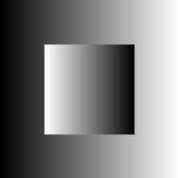
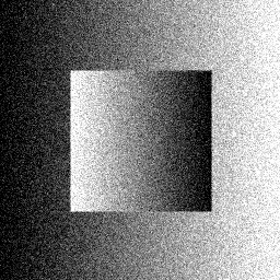
test image [8]		with Gaussian noise ($\sigma=40$)
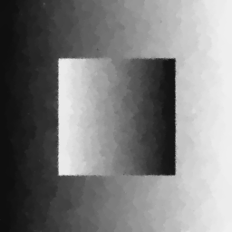
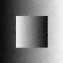
TV (MSE: 35.06)		ours, 1st order (MSE: 31.79)
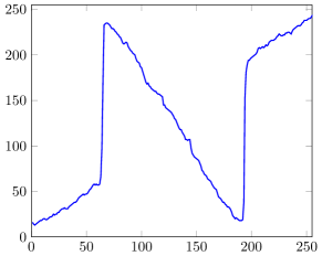
row 87, TV model		row 87, 1st order model

Figure 1: Comparison of denoising result for first order models

In this section we discuss the application of our first and second order coupling models for denoising. We compare our models to TV denoising [24] and the combined first and second order approach TV-TV² by Papafitsoros et al. [23]. We set the regularisation parameter of the penalising function to $\epsilon=10^{-6}$ and stop the algorithms if the relative residuum gets smaller than $10^{-6}$. For the solution of the linear subproblems we perform an inner loop of $10$ Jacobi steps per iteration. The numerical parameter $\lambda$ is important for the number of iterations until convergence is reached. Empirically we found that $\lambda$ should be chosen in dependence of $\beta$ and the regularisation order $\ell$. We fix $\lambda:=\ell\cdot\beta$. We choose the parameters optimally for each method such that the mean squared error (MSE) w.r.t. the ground truth is minimised.

In Fig. 1 we consider an affine test image of size $256\times 256$ that is corrupted by Gaussian noise with $\sigma=40$. We first consider denoising by first order models. Our model is able to beat the classical TV model w.r.t. the MSE. We also see a qualitative improvement when we consider a horizontal cross section of the images in the last row. We reduce the staircasing artifacts significantly.

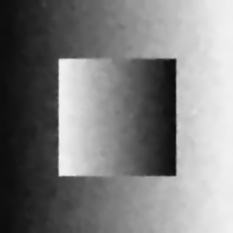
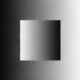
TV-TV2 (MSE: 31.35)		ours, 2nd order (MSE: 26.02)
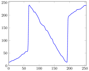
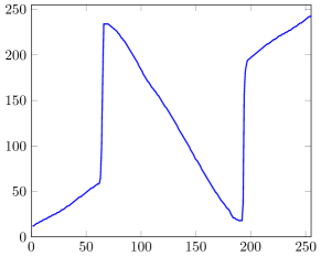
row 87, TV-TV2 model		row 87, 2nd order model

Figure 2: Comparison of denoising result for second order models

We compare the reconstruction by second order models in Fig. 2. While the TV-TV² model beats our first order coupling model only slightly w.r.t. to the MSE, our second order model presents a large improvement. In the 1D plot we see that no staircasing artifacts arise.

This experiment also illustrates the efficiency of the split Bregman implementation for solving our problems. We compare two implementations. On the one hand we employ an alternating minimisation strategy of equations (21) and (22) resp. (23) realised with a standard conjugate gradient method. On the other hand we apply a split Bregman Implementation based on the subproblems that arise from equation (25).

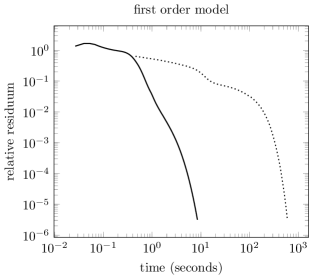
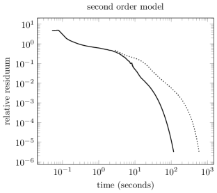
Figure 3: A log-log plot of runtime comparison of implementation with conjugate gradient scheme (dotted) and split Bregman implementation (straight line).

Figure 3 shows the decay in the relative residuum as a function to the runtime. For both the first and second order model, we gain a speed up of more than one order of magnitude with the split Bregman scheme.

4.2 Convex Mumford-Shah Approximation

To understand how the coupling model approximates the Mumford-Shah functional we first have to discuss the influence of the parameters. The parameter $\beta$ determines the smoothness between segments. For a fixed value of $\alpha$, increasing $\beta$ reduces the number of segments and consequently of detected edges. To counteract the segment fusion steered by $\beta$, the parameter $\alpha$ should be chosen relatively large to benefit from the TV-like effect inside each segment.

In Fig. 4 we show our first order model for varying values of $\beta$ together with the edge set that we get from the coupling term. For better visualisation we perform a hysteresis thresholding of the edge set [12]. Our method is able to produce smooth segments. For an increasing value of $\beta$, more and more segments are merged. For instance we see that the smaller hole in the rock vanishes for a higher value. As already mentioned the resulting images are rather smooth in each segment due to the quadratic smoothness term, but we still have sharp edges in between. For an increasing $\beta$ value we obtain a sparser edge set.

original image [14]	$\alpha=750$, $\beta=50$	$\alpha=750$, $\beta=500$

Figure 4: First row: original image and segmentation results for our first order model. Second row: corresponding edge sets $\|\bm{\nabla}\bm{u}-\bm{v}\|^{2}$.

4.3 Application to Edge Detection

The previous subsection shows that an edge detector can be obtained directly from the coupling term. In Fig. 5 we illustrate its high robustness under noise. We compare it to a Canny edge detector [12], which is a classical edge detection method. To compensate for the noise, the Canny edge detector presmoothes the image by a convolution with a Gaussian kernel. While most large scale structures are detected, edges of smaller details are dislocated or merged together. This can be seen e.g. at the branch below the bird. Our method works edge-preserving and is able to capture these small details.

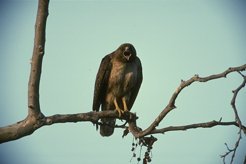
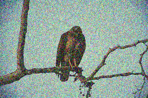
Figure 5: First row: Original image [14]; noisy version ($\sigma=100$) second row: edge set of the Canny edge detector; edge set of our first order model.

5 Conclusions and Outlook

We have shown that coupling terms in variational models are useful for more than just easing numerics. Already first order models that contain a coupling term in the sparsity promoting $L^{1}$ norm are sufficient for edge-preserving denoising. For the remaining data and smoothness terms we can use simple quadratic $L^{2}$ norms. This does not only simplify the numerical minimisation scheme, it also challenges the common belief that edge-preserving denoising requires a nonquadratic smoothness term. The first order coupling model also shows a theoretical connection to the classical segmentation model of Mumford and Shah. As it works on a strictly convex energy, we obtain an approximation of the Mumford-Shah functional that has a unique solution and is guaranteed to converge. Furthermore, the introduced coupling term itself carries valuable information: It has the properties of a global edge detector that is robust against noise and comes at literally no cost as a byproduct of the minimisation.

In our ongoing research we investigate how the coupling formulation can be extended to applications in deblurring or inpainting or in combination with anisotropic regularisation. Moreover, we intend to exploit the simplicity of the quadratic terms by using parallel implementations to gain more efficient solvers.

References

- [1] R. Acar and C. R. Vogel. Analysis of bounded variation penalty methods for ill–posed problems. Inverse Problems, 10:1217–1229, 1994.
- [2] L. Ambrosio, N. Fusco, and D. Pallara. Functions of Bounded Variation and Free Discontinuity Problems. Oxford University Press, Oxford, 2000.
- [3] L. Ambrosio and V. Tortorelli. Approximation of functionals depending on jumps by elliptic functionals via -convergence. Bolletino della Unione Matematica Italiana, 7:105–123, 1992.
- [4] M. Bildhauer, M. Fuchs, and J. Weickert. An alternative approach towards the higher order denoising of images. analytical aspects. Journal of Mathematical Sciences, 224(3):414–441, July 2017.
- [5] A. Blake and A. Zisserman. Visual Reconstruction. MIT Press, Cambridge, MA, 1987. Paperback reprint edition.
- [6] S. Boyd, N. Parikh, B. Peleato, and J. Eckstein. Distributed optimization and statistical learning via the alternating direction method of multipliers. Foundations and Trends in Machine Learning, 3:1–122, 2010.
- [7] K. Bredies, K. Kunisch, and T. Pock. Total generalized variation. SIAM Journal on Imaging Sciences, 3(3):492–526, 2010.
- [8] E.-M. Brinkmann, M. Burger, and J. S. Grah. Unified models for second-order TV-type regularisation in imaging-a new perspective based on vector operators. Journal of Mathematical Imaging and Vision, 61(5):571–601, June 2019.
- [9] M. Burger, T. Esposito, and C. I. Zeppieri. Second-order edge-penalization in the ambrosio–tortorelli functional. Multiscale Modeling & Simulation, 13(4):1354–1389, 2015.
- [10] M. Burger, K. Papafitsoros, E. Papoutsellis, and C. Schönlieb. Infimal convolution regularisation functionals of BV and spaces. part I: The finite case. Journal of Mathematical Imaging and Vision, 55(3):343–369, July 2016.
- [11] X. Cai, R. Chan, and T. Zeng. A two-stage image segmentation method using a convex variant of the Mumford–Shah model and thresholding. SIAM Journal on Imaging Sciences, 6(1):368–390, 2013.
- [12] J. Canny. A computational approach to edge detection. IEEE Transactions on Pattern Analysis and Machine Intelligence, 8:679–698, 1986.
- [13] A. Chambolle and P.-L. Lions. Image recovery via total variation minimization and related problems. Numerische Mathematik, 76:167–188, 1997.
- [14] D. Martin, and C. Fowlkes. Berkeley Segmentation and Boundary Detection Benchmark and Dataset. http://www.cs.berkeley.edu/projects/vision/grouping/segbench., 2003.
- [15] J. Duan, Y. Ding, Z. Pan, J. Yang, and L. Bai. Second order Mumford–Shah model for image denoising. In Proc. 2015 IEEE International Conference on Image Processing, pages 547–551, Sep. 2015.
- [16] T. Goldstein and S. Osher. The split Bregman method for L1-regularized problems. SIAM Journal on Imaging Sciences, 2(2):323–343, 2009.
- [17] D. Hafner, C. Schroers, and J. Weickert. Introducing maximal anisotropy into second order coupling models. In J. Gall, P. Gehler, and B. Leibe, editors, Pattern Recognition, volume 9358 of Lecture Notes in Computer Science, pages 79–90. Springer, Cham, 2015.
- [18] A. Hewer, J. Weickert, T. Scheffer, H. Seibert, and S. Diebels. Lagrangian strain tensor computation with higher order variational models. In T. Burghardt, D. Damen, W. Mayol-Cuevas, and M. Mirmehdi, editors, Proc. 24th British Machine Vision Conference, pages 129.1–129.10, Bristol, Sept. 2013. BMVA Press.
- [19] B. K. P. Horn. Height and gradient from shading. International Journal of Computer Vision, 5(1):37–75, 1990.
- [20] J. M. Hyman and M. Shashkov. Natural discretizations for the divergence, gradient, and curl on logically rectangular grids. Computers and Mathematics with Applications, 33(4):81–104, 1997.
- [21] M. Lysaker, A. Lundervold, and X.-C. Tai. Noise removal using fourth-order partial differential equations with applications to medical magnetic resonance images in space and time. IEEE Transactions on Image Processing, 12(12):1579–1590, Dec. 2003.
- [22] D. Mumford and J. Shah. Optimal approximation of piecewise smooth functions and associated variational problems. Communications on Pure and Applied Mathematics, 42:577–685, 1989.
- [23] K. Papafitsoros and C. B. Schönlieb. A combined first and second order variational approach for image reconstruction. Journal of Mathematical Imaging and Vision, 48(2):308–338, Feb 2014.
- [24] L. I. Rudin, S. Osher, and E. Fatemi. Nonlinear total variation based noise removal algorithms. Physica D, 60:259–268, 1992.
- [25] O. Scherzer. Denoising with higher order derivatives of bounded variation and an application to parameter estimation. Computing, 60:1–27, 1998.
- [26] S. Setzer. Split Bregman algorithm, Douglas-Rachford splitting and frame shrinkage. In X.-C. Tai, K. Mørken, M. Lysaker, and K.-A. Lie, editors, Scale Space and Variational Methods in Computer Vision, pages 464–476. Springer, 2009.
- [27] S. Setzer, G. Steidl, and T. Teuber. Infimal convolution regularizations with discrete 1-type functionals. Communications in Mathematical Sciences, 9(3):797–872, 2011.
- [28] A. N. Tikhonov. Solution of incorrectly formulated problems and the regularization method. Soviet Mathematics Doklady, 4:1035–1038, 1963.
- [29] E. T. Whittaker. A new method of graduation. Proceedings of the Edinburgh Mathematical Society, 41:65–75, 1923.
- [30] Y.-L. You and M. Kaveh. Fourth-order partial differential equations for noise removal. IEEE Transactions on Image Processing, 9(10):1723–1730, 2000.