Quantum Absorbance Estimation and the Beer-Lambert Law

Abstract

The utility of transmission measurement has made it a target for quantum enhanced measurement strategies. Here we find if the length of an absorbing object is a controllable variable, then via the Beer-Lambert law, classical strategies can be optimised to reach within 83% of the absolute quantum limit. Our analysis includes experimental losses, detector noise, and input states with arbitrary photon statistics. We derive optimal operating conditions for both classical and quantum sources, and observe experimental agreement with theory using Fock and thermal states.

In sensing scenarios, a measured parameter is often a function of known constants of the experiment and the particular variable of interest. An example of this is the Beer-Lambert law, where the intensity of radiation transmitted through a sample of length $L$ is given by: $I=~{}I_{0}\exp{(-aL)}$, where $I_{0}$ and $I$ are the intesities before and after the sample, and $a$ is the sample absorbance parameter. The law is ubiquitous across a wide range of investigative techniques including atomic vapour thermometry Truong et al. (2011), femtosecond pump-probe spectroscopy Woutersen et al. (1997), high-throughput screening Inglese et al. (2007), on- and in-line food processing Scotter (1990), medical diagnostics Behera et al. (2012), and spectrophotometry Trumbo et al. (2013). The Beer-Lambert law also applies to non-optical techniques such as neutron transmission and electron tomography Vontobel et al. (2006); Yan et al. (2015).

Optical quantum metrology investigates how quantum strategies, such as probing with quantum states of light, provides increased precision over classical techniques in estimating parameters including optical phase Caves (1981); Ono et al. (2013), transmission Sabines-Chesterking et al. (2017); Moreau et al. (2017), polarisation Zhang et al. (2016), and displacements Braginsky (1967). A variety of practical implementations have demonstrated these schemes and have been shown to outperform classical strategies operating at the same average input intensity Aasi et al. (2013).

Motivated by the utility of measuring optical absorption to image and identify objects, there has been a series of studies exploring the benefits of using quantum light to estimate the total transmission $\eta$, where the average intensity passing through the loss channel is ${I}=\eta{I}_{0}$ Fujiwara (2004); Adesso et al. (2009); Brida et al. (2010); Moreau et al. (2017). Here, we investigate how the advantage of applying optimal quantum states changes, if the parameter sought is the absorbance coefficient $a$ (loss per unit length) used in the Beer-Lambert law Whittaker et al. (2017).

The scenario we consider (Fig. 1) comprises the targeted absorbance $a\in(0,\infty)$, a variable length $L\in(0,\infty)$, length independent loss $\gamma$ which, for example, could arise from loss at each facet of the sample chamber, and a length dependent loss per unit length $\beta$, which we refer to as co-propagating loss, and could arise from a distinct absorbing material in the chamber with the sample. Input intensity $I_{0}$ is then related to output $I$ by

$$I=I_{0}\exp(-aL)\eta_{l},$$ (1)

where we group the instrumental ‘non-sample’ loss mechanisms as $\eta_{l}=\gamma^{2}\exp(-\beta L)$ and facet loss is assumed to be the same for entrance and exit to simplify expressions. Variables $L$, $\beta$, and $\gamma$ are assumed to be known a priori to infinite precision and so contribute no uncertainty to estimating $a$. We note that both length dependent loss variables $a$ and $\beta$ are multiplied by the same length $L$ as any loss occurring outside of $L$ can be encapsulated in the parameter $\gamma$.

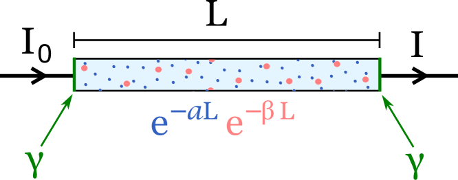
Figure 1: A typical experiment to measure the absorbance of a medium in the presence of other loss mechanisms such as surface losses $\gamma$ and co-propagation loss $\beta$.

To compare different experimental strategies, we use the Fisher information per average incident photon into the sample, $\mathcal{F(x)}=F(x)/N_{0}$, where $F(x)$ is the total Fisher information for the probe state on the parameter $x$ and $N_{0}$ is the mean input photon number. Using Fisher information per absorbed photon, $F/(N_{0}(1-\eta))$, does not alter the qualitative results observed but can alter the optimal numerical values of parameters (which can still be analytically defined).

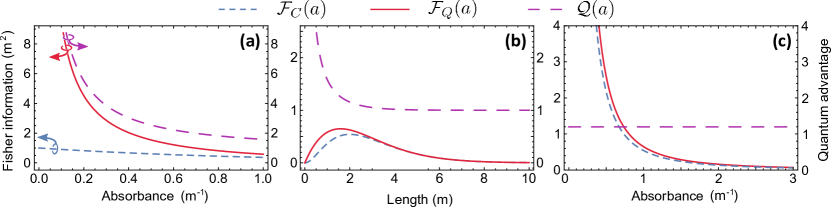
Figure 2: (a) $\mathcal{F}(a)$ given a fixed $L=1$ for both classical and quantum strategies. Also shown is the quantum advantage $\mathcal{Q}(a)$ (ratio of quantum to classical Fisher information). The trend follows that previously found from absorption estimation, where weakly absorbing samples are most improved by using quantum states of light. Colour arrows dictate relevant axis for each line. (b) $\mathcal{F}(a)$ and quantum advantage $\mathcal{Q}(a)$ given a fixed sample absorbance of $a=1$. We see that the Fisher information in both classical and quantum cases peaks at particular length values. (c) $\mathcal{F}(a)$ and quantum advantage $\mathcal{Q}(a)$ when both schemes are allowed to operate at the optimal length values given by Eq. 8 and 9. We see that maximising the Fisher information in the classical and quantum case means that the quantum advantage is fixed to a value of $1.2$ for all values of absorbance.

For estimation of the total absorption $\eta$, the best known quantum strategy is to input Fock states, $\ket{N_{0}}$, of known photon number $N_{0}$ into the sample, and measure the output intensity Fujiwara (2004); Adesso et al. (2009). The corresponding classical strategy uses a coherent state $\ket{\alpha}$, with mean photon number $N_{0}=|\alpha|^{2}$. While absorbance and absorption estimation differ in parametrisation, in both cases the underlying evolution of any input quantum state is the same physical process of a loss channel. Therefore the Fisher information of absorption and absorbance are proportional to one another (Eq. 2) Lehmann and Casella (2006); Paris (2009), and so share the same optimal quantum and classical strategies. We therefore can consider the difference between these two input states as defining the difference between classical ($\ket{\alpha}$ input) and quantum ($\ket{N_{0}}$ input) strategies in absorbance estimation.

Because $\eta=\exp(-aL)$ is a continuous differentiable function of $a$, the relationship relating the Fisher information on each parameter applies Lehmann and Casella (2006):

$$\mathcal{F}(a) =\left(\frac{\partial\eta}{\partial a}\right)^{2}\mathcal{F}(\eta)$$ (2)

$$=L^{2}e^{-2aL}\mathcal{F}(\eta).$$

For absorption estimation with $\eta_{l}$ present, for classical and quantum strategies, we have sup

$$\mathcal{F}_{C}(\eta)=\frac{\eta_{l}}{\eta}=\eta_{l}e^{aL},$$ (3)

$$\mathcal{F}_{Q}(\eta)=\frac{\eta_{l}}{\eta(1-\eta\eta_{l})}=\frac{\eta_{l}e^{aL}}{1-\eta_{l}e^{-aL}}.$$ (4)

When combined with Eq. 2, Eqs. 16, & 17 provide Fisher information per incident photon for estimating $a$

$$\mathcal{F}_{C}(a)=L^{2}\gamma^{2}e^{-(a+\beta)L},$$ (5)

$$\mathcal{F}_{Q}(a)=\frac{L^{2}\gamma^{2}}{e^{(a+\beta)L}-\gamma^{2}}.$$ (6)

These are plotted in Fig. 2(a) for a fixed $L=1$ and no experimental loss $\eta_{l}=1$, along with the quantum advantage $\mathcal{Q}(a)=\mathcal{F}_{Q}(a)/\mathcal{F}_{C}(a)$. We see that fixing $L$ provides a scaling for $\mathcal{Q}(a)$ that follows the trend of absorption estimation, namely that $\mathcal{Q}(a)\rightarrow\infty$ for $a\rightarrow 0$ ($\mathcal{Q}(\eta)\rightarrow\infty$ for $\eta\rightarrow 1$) Sabines-Chesterking et al. (2017).

We see in Fig. 2(b) how $\mathcal{F}(a)$ changes for a fixed sample absorbance ($a=1$), no experimental loss $\eta_{l}=1$ and a varying $L$. This behaviour differs from Fig. 2(a). For a varying length we see that both $\mathcal{F}_{C}(a)$ and $\mathcal{F}_{Q}(a)$ have maximal values before tending towards zero for both large and small $L$. This demonstrates that for a particular $a$ (e.g. a particular gas fixed in concentration), optimising the length of the medium that the light passes through provides maximum information on $a$. For the classical Fisher information provided in Eq. 5, the optimum can be found by solving ${\partial\mathcal{F}_{C}(a)}/{\partial L}=0$:

$$\frac{\partial\mathcal{F}_{C}(a)}{\partial L} =2L\gamma^{2}e^{-(a+\beta)L}-(a+\beta)L^{2}\gamma^{2}e^{-(a+\beta)L}$$

$$=(2-(a+\beta)L)L\gamma^{2}e^{-(a+\beta)L}=0,$$ (7)

which for non-zero $L$ and $a$, is only satisfied for $(a+\beta)L=2$. Therefore for a coherent state

$$L_{\text{opt}}^{C}={2}/{(a+\beta)},$$ (8)

maximises $\mathcal{F}_{C}(a)$. For $a=1$, $\beta=0$, and $\gamma=1$, this is in agreement with Fig. 2(b). An identical process for $\mathcal{F}_{Q}(a)$ yields the optimal

$$L_{\text{opt}}^{Q}=\frac{\mathcal{W}\left[-2\gamma^{2}/e^{2}\right]+2}{a+\beta},$$ (9)

where $\mathcal{W}[x]$ is the principal value of the Lambert W-function Corless et al. (1996). As the values of $L_{\text{opt}}$ are inversely proportional to $a$, the optimal lengths correspond to constant total absorption values. For $\beta=0$ and $\gamma=1$, these are $\eta_{\text{optimal}}^{Q}=0.20$ and $\eta_{\text{optimal}}^{C}=0.14$. This shows that for any fixed $a$, $L$ should be chosen to provide approximately $\geq$80% total absorption through the sample.

We now compare $\mathcal{F}_{C}(a)$ and $\mathcal{F}_{Q}(a)$ when both schemes are allowed their optimal $L_{\text{opt}}$ value. We compute the quantum advantage as a function of absorbance where at each value of $a$ the length of the material is set to $L_{\text{opt}}(a)$, and arrive at Fig. 2(c). Here we see that in the case where there are no constraints on $L$, the advantage gained by using quantum states of light is limited to a fixed factor of $\mathcal{Q}(a)=1.2$ for any $a$. Alternatively, this shows that classical light can reach to within $83\%$ of the fundamental quantum bound. This shows free choice of the length parameter $L$ can severely limit the benefit of implementing a quantum strategy for estimating the absorbance. This effect can also be seen analytically by inputting the respective values for $L_{\text{opt}}$ into the expression for quantum advantage.

An important feature of $L_{\text{opt}}$ is that for both strategies it is a function of the absorbance. Since $a$ is the parameter being estimated, there are cases where it will not be known in advance. There do, however, exist practical scenarios when one may still be able to implement $L_{\text{opt}}$. One is when the experiment is intended to measure a deviation from an initially known $a$ by $\delta a$, such as a change in the concentration of a gas. Another scenario is when $a$ is known approximately and the quantum strategy is employed to achieve a more precise measurement of its value. Finally, in cases when $a$ is completely unknown beforehand but $L$ can be easily varied, one could use Bayesian inference to adaptively update the value of $L$ as an estimate of $a$ is attained, eventually arriving at the value $L_{\text{opt}}$.

In the classical case, $L_{\text{opt}}$ is independent of $\gamma$ and so is independent of facet loss. When both schemes are operated with their respective $L_{\text{opt}}$, the quantum advantage is found to be independent of $\beta$. The absolute Fisher information for each scheme is reduced as a co-propagating loss is introduced (non-zero $\beta$) but they are reduced by the same amount such that the ratio, $\mathcal{Q}(a)$, remains unchanged. This is not the case for the value of $\gamma$, which has a more detrimental effect on $\mathcal{F}_{Q}(a)$ than it does on $\mathcal{F}_{C}(a)$. Supplementary Material B sup displays how the quantum advantage is changed as $\gamma$ is varied.

We now expand our analysis to consider states more general than Fock and coherent states $\ket{\psi}$, with arbitrary Fano factor $\sigma_{{\psi}}=\mathrm{Var}(N_{{0}})/\bar{{N}}_{{0}}$ where $\mathrm{Var}(N_{{0}})$ and $\bar{{N}}_{{0}}$ are the input photon number variance and mean respectively. This allows the estimation capabilities of any light source with any statistics to be found. In Supplementary Material C sup we investigate estimation bounds in total absorption estimation when considering general input states of light and find that the Fisher information on the transmission $\eta$ is given by

$$\mathcal{F}_{\psi}(\eta)=1/{\left(\eta^{2}\sigma_{{\psi}}+\eta(1-\eta)\right)},$$ (10)

where for simplicity we have assume $\eta_{l}=1$. Following the same analysis as the Fock and coherent state inputs, where the Fisher information in $\eta$ is related to the Fisher information of $a$ using Eq. 2, the Fisher information is found to be

$$\mathcal{F}_{\psi}(a)={L^{2}}/{\left(\sigma_{{\psi}}+\exp(aL)-1\right)}.$$ (11)

For the specific cases of the coherent and Fock states ($\sigma_{{\psi}}=1$ and $0$ respectively), $\mathcal{F}_{\psi}(a)$ returns to $\mathcal{F}_{C}(a)$ and $\mathcal{F}_{Q}(a)$. The dependence of the optimal length on $\sigma_{{\psi}}$ is found analytically to be

$$L_{\text{opt}}^{{\psi}}=\left(\mathcal{W}\!\left[{2(\sigma_{{\psi}}-1)}/{e^{2}}\right]+2\right)/a.$$ (12)

The general features of absorbance estimation also appear in multipass or multi-application strategies for quantum and classical light. Specifically, the freedom of multiple passes acts like a discrete version of optimising the length and allows the classical scheme to reach close to the estimation capabilities of the quantum strategy. We show this in Supplementary Material D sup by revisiting work by Birchall et al. who investigated multipass strategies in lossy phase estimation Birchall et al. (2017) and loss estimation Birchall et al. (2019). We investigate the problem of estimating a sample transmission $\epsilon$ that is interrogated multiple times by either applying $\epsilon$ $i$ times to the beam (with $i$ copies of $\epsilon$), or by passing light through the same sample $i$ times, such that the total loss on the optical beam is $\eta=\epsilon^{i}$.

We experimentally demonstrate the length dependent optimisation that can be performed for both quantum (single photon) and noisy (thermal) sources of light using the experimental setup illustrated in Fig. 3(a). A collinear type II spontaneous parametric down conversion (SPDC) source (periodically-poled potassium titanyl phosphate/PPKTP crystal) is pumped by a 3 mW 404 nm continuous-wave (CW) laser and spontaneously produces correlated photon pairs at 810 nm that have orthogonal polarisations. The spectral output of the crystal is controlled by varying the temperature using an oven. The pair of photons are spatially separated at a PBS into the ‘signal’ and ‘idler’ channels. The signal photon is detected by a single photon avalanche photodiode (SPAD) which heralds the presence of the other photon, producing a single photon Fock state. Long pass (LPF) and band pass filters (BPF) are used to filter out the pump.

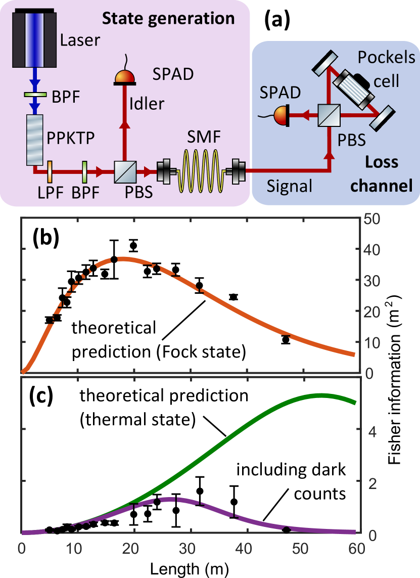
Figure 3: (a) Experimental setup to measure optimisation of sample length (b) Results for pair-photon source (c) Results for single-armed source with and without dark counts included in the theoretical analysis.

The sample of varying loss is implemented using a Pockels cell modulator composed of two lithium niobate crystals. When inactive, these crystals rotate the polarisation of the photon by 90 degrees but cause no rotation when activated. When used in conjunction with a polarising beamsplitter (PBS), this applies a variable loss to the incoming photon. At the wavelength of interest, the halfway voltage of the device is 200 V and so the crystal is driven by a high voltage driver. To make the loss independent to the photon input polarisation (which is arbitrary due to the single-mode optical fibre prior to the loss channel), we used the Sagnac configuration from Sabines-Chesterking et al. (2017). The transmission of the idler photon’s path with the switch fully open is 38%, including detection efficiency, and thus we apply $\gamma=\sqrt{0.38}=0.62$ and $\beta=0$ to the following analysis. The experiment produced approximately 14 k coincidences/s.

Optimisation of $L$ is observed by applying the inferred total loss from an object with absorbance $a=1$ m^-1 with varying $L$. For example, for $a=1$ m^-1, $L=\{1,3,5\}$ m applies losses $\eta=\exp{(-aL)}=\{0.37,0.14,0.05\}$, that we implement with the Pockels cell. By setting each $\eta$ and then taking measurements to estimate $a$ (given that we have prior knowledge of $L$), we measure the statistics of the noise on the estimate of absorbance and hence estimate $\mathcal{F}(a)=1/\mathrm{Var}(\hat{a})$, where $\mathrm{Var}(\hat{a})$ denotes the variance on the estimates of the parameter $a$.

Estimates of $a$ are found by using the estimator

$$\hat{a}=-\log\left({N_{cc}}/{\gamma N_{S}}\right)/L,$$ (13)

where $N_{cc}$ is the number of coincidences between the signal and idler detectors, and $N_{S}$ is the total number in the signal channel. This is an adaptation of the estimator used for absorption estimation with pair sources and photon counting Sabines-Chesterking et al. (2017). Eq. 13 is only valid for the Fisher information per incident photon metric where instrumental loss occurring before and after the sample affect $\mathcal{F}$ in the same fashion, and therefore do not need to be considered independently. A total of 500 estimates for each setting of absorbance were found using a coincidence window of 0.5 seconds. These were separated into five groups of 100 estimates, and the variance of each group computed each providing a Fisher information estimate. The mean of these are shown in Fig. 3(b) and error bars are computed using the standard error of these Fisher information estimates. These show good agreement with theoretical predictions for the Fock state strategy.

By disregarding the idler photons we experimentally test the estimation capabilities of a noisy (thermal) light source as a single arm of a pair photon source is a thermal state Blauensteiner et al. (2009). In this case, the estimator for the absorbance is changed to

$$\hat{a}=-\log\left[\left({N_{I}-{N}_{DC}}\right)/{\bar{N}_{0}}\right]/L,$$ (14)

where $N_{I}$ is the number of idler photons detected, $N_{DC}$ is the mean number of dark counts in the idler detector, and $\bar{N}_{0}$ is the mean number of input photons, found prior by applying no loss.

The experimental results in Fig. 3(c) deviate from the theory given by Eq. 10. We attribute this to dark counts from the detectors, which are particularly detrimental for the thermal state (single arm) strategy as the counts from the lossy arm are used to estimate $\eta$. This is in contrast to the more robust coincidence estimator (Eq. 13) where only the singles in the signal channel are considered. By adding dark counts into the analysis of the Fisher information (Supplementary Material E sup ) we are able to reconcile the difference between the theoretical prediction and the experimental results seen in Fig. 3(c). We estimate the $\sigma_{\psi}$ value for the idler path by measuring the photon number variance and mean when there is no sample present and correcting for the inherent loss of the channel (see Supplementary Material F sup ). This gave a predicted $\sigma_{\psi}=826$.

Including dark counts provides an estimator information per incident photon of

$$I(\eta)=\left[\mathrm{Var}(N_{DC})/{\bar{N}_{0}}+\eta^{2}\sigma_{\psi}+(1-\eta)\eta\right]^{-1},$$ (15)

where $\mathrm{Var}(N_{DC})$ is the variance of the detector dark counts. We expect this estimator information bound to be optimal (and hence equal to the Fisher information), but have no rigorous proof of this. $\mathrm{Var}(N_{C})$ in this experiment was measured to be 518 $s^{-2}$.

We have shown how experimental optimisation of the sample length $L$ can offer significant advantages in precision for both quantum and classical inputs in absorbance estimation. We find that for cases where this optimisation is possible, the quantum advantage is restricted to $1.2$ at most. We have derived optimal operating conditions for a number of experimental variations including additional experimental loss, input states with arbitrary photon number statistics, and detector dark counts. The experimental implementation presented demonstrates that $L$ can be optimised for Fock and thermal states, suggesting that for such an experiment the quantum advantage would be limited. These results not only have implications for future quantum sensors designed for measuring absorbance but can also be applied to optimise current classical sensors using laser or thermal light.

The existence of experimental optimisation strategies for absorbance, phase Birchall et al. (2017), and loss estimation Birchall et al. (2019); sup , suggest that in general the existence of a free optimisation parameter can be a powerful tool for increasing the achievable measurement precision. Future analysis and experiments should consider this in order to correctly predict the advantage provided by quantum strategies. Efforts towards providing practical advantages using quantum states of light can now be focussed towards applications where such optimisation strategies are difficult to implement, such as imaging or very weakly absorbing samples.

I Supplementary Material

I.1 Supplementary Material A: Total Absorption ($\eta$) Estimation with Loss

It has previously been shown Whittaker et al. (2017); Sabines-Chesterking et al. (2017) that for transmission estimation, where the goal is to estimate a transmission $\eta$ defined by the input $I_{0}$ and output intensity $I=\eta I_{0}$, the Fisher information per incident photon for a coherent and Fock state input are given respectively to be

$$\mathcal{F}_{C}(\eta) =\frac{1}{\eta},$$ (16)

$$\mathcal{F}_{Q}(\eta) =\frac{1}{\eta(1-\eta)},$$ (17)

where $\mathcal{F}$ bounds the variance on any unbiased estimate of $\eta$ via

$$\mathcal{F}(\eta)\leq\frac{1}{\mathrm{Var}(\hat{\eta})},$$ (18)

where $\hat{\eta}$ denotes an estimator of the parameter $\eta$. We note that these bounds were derived for the case where no experimental loss (other than for the sample $\eta$) exists. Here we derive how these bounds are changed by the introduction of experimental loss is also applied to the channel (e.g. by inefficient detectors). This loss is characterise by a second transmission parameter $\eta_{l}$ such that the input and output intensities are defined by $I=\eta\eta_{l}I_{0}$.

Assuming no change to the photon energy through the experiment, the output photon number from the lossy channel is given by

$$\bar{N}=\eta\eta_{l}\bar{N}_{0}$$ (19)

where $\bar{N}_{0}$ and $\bar{N}$ are the mean input and output photon numbers respectively. Considering the estimator $\hat{\eta}=N/(\eta_{l}\bar{N}_{0})$ (which has previously been show to saturate the Fisher information bound Whittaker et al. (2017); Sabines-Chesterking et al. (2017)) and using the error propagation formula: $\mathrm{Var}(\hat{\eta})=\left(\frac{\partial\eta}{\partial N}\right)^{2}\mathrm{Var}(N)$ we can relate the variance on any estimate of $\hat{\eta}$ to the output photon number variance and find

$$\mathrm{Var}(\hat{\eta})=\frac{\mathrm{Var}(N)}{(\eta_{l}\bar{N}_{0})^{2}}.$$ (20)

For an input coherent state $\ket{\alpha}$ ($|\alpha|^{2}=N_{0}$) input into a lossy channel, the output state is given by $\ket{\sqrt{\eta_{l}\eta}\alpha}$ and therefore the photon number statistics at the output follow a Poisson distribution with a characteristic variance equivalent to the it’s mean $\mathrm{Var}(N)_{C}=\eta_{l}\eta N_{0}$. Similarly, a Fock state input will have output statistics defined by a Binomial distribution Whittaker et al. (2017) with number of trials $N_{0}$ and success probability (chance of being transmitted) $\eta\eta_{l}$. As a result, for a Fock state — the optimal quantum strategy — the output photon number variance is given by $\mathrm{Var}(N)_{Q}=\eta_{l}\eta(1-\eta_{l}\eta)\bar{N}_{0}$.

Combining the classical and quantum output photon number variances with Equation 20 and using $\mathcal{F}^{\prime}(\eta)=1/(\mathrm{Var}(\hat{\eta})\bar{N}_{0})$ we find

$$\mathcal{F}_{C}(\eta) =\frac{\eta_{l}}{\eta},$$ (21)

$$\mathcal{F}_{Q}(\eta) =\frac{\eta_{l}}{\eta(1-\eta\eta_{l})},$$ (22)

as defined in the main text.

I.2 Supplementary Material B: Quantum Advantage as a Function of the Loss Parameter $\gamma$

Figure 4 demonstrates how the quantum advantage varies as a function of the length independent facet transmission $\gamma$ (defined in the main text). We see that unlike the length dependent loss factor $\beta$ the quantum advantage offered by Fock states is reduced as the transmission $\gamma$ is reduced.

Figure 4: The quantum advantage in estimation the absorbance as a function of the experimental transmission value $\gamma$. The value of $\gamma$ provides the value of the length independent loss, applied twice for loss occurring before and after the sample of interest.

I.3 Supplementary Material C: Absorption Estimation with Arbitrary Input States

Here we derive the Fisher information attained on $\eta$ when arbitrary states, $\ket{\psi}$ characterised by the Fano factor $\sigma_{{\psi}}=\mathrm{Var}(N_{{0}})/\bar{N}_{0}$ where $\mathrm{Var}(N_{{0}})$ and $\bar{N}_{0}$ are the input photon number variance and mean respectively, are incident on the absorbing medium.

Let $X({N}_{0})$ define the (arbitrary) photon number distribution describing the input state of light used to probe a sample of transmission $\eta$ where ${N}_{0}$ is the input photon number. As we are interested in linear absorption processes, where the loss acts independently on each incoming photon, passing this light through the sample applies a Binomial distribution to the input distribution and results in the output compound distribution

$$\mathcal{X}_{B}(N|\eta)=\sum_{{N}_{0}=0}^{\infty}X({N}_{0})B(N|{N}_{0},\eta),$$ (23)

where $B(N|{N}_{0},\eta)$ defines a binomial distribution providing the probability of measuring $N$ sucesses with ${N}_{0}$ trials and a chance of success of $\eta$. The expectation values and variance of the Binomial distribution

$$B(N|{N}_{0},\eta)={{N}_{0}\choose N}\eta^{N}(1-\eta)^{{N}_{0}-N},$$ (24)

can be calculated to be:

$$\mathds{E}_{B}[N] =\sum_{N=0}^{\infty}NB(N|{N}_{0},\eta)={N}_{0}\eta,$$ (25)

$$\mathds{E}_{B}[N^{2}] =\sum_{N=0}^{\infty}N^{2}B(N|{N}_{0},\eta)$$

$$={N}_{0}\eta+{N}_{0}^{2}\eta^{2}-{N}_{0}\eta^{2}$$ (26)

$$=\eta^{2}{N}_{0}^{2}+\eta(1-\eta){N}_{0},$$ (27)

$$\mathrm{Var}_{B}(N) =\mathds{E}_{B}[N^{2}]-\mathds{E}_{B}[N]^{2}$$ (28)

$$={N}_{0}\eta-{N}_{0}\eta^{2}={N}_{0}\eta(1-\eta),$$ (29)

where $\mathds{E}_{F}[x]$ denotes the expectation value of $x$ for the distribution $F$. For the compound distribution $\mathcal{X}_{B}(N|\eta)$:

$$\mathds{E}_{\mathcal{X}_{B}}[N] =\sum_{N=0}^{\infty}N\mathcal{X}_{B}(N|\eta)$$

$$=\sum_{N=0}^{\infty}N\sum_{{N}_{0}=0}^{\infty}X({N}_{0})B(N|{N}_{0},\eta)$$

$$=\sum_{{N}_{0}=0}^{\infty}X({N}_{0})\mathds{E}_{B}[N]$$

$$=\sum_{{N}_{0}=0}^{\infty}X({N}_{0}){N}_{0}\eta=\eta\mathds{E}_{X}[{N}_{0}],$$

$$\mathds{E}_{\mathcal{X}_{B}}[N^{2}] =\sum_{N=0}^{\infty}N^{2}\sum_{{N}_{0}=0}^{\infty}X({N}_{0})B(N|{N}_{0},\eta)$$

$$=\sum_{{N}_{0}=0}^{\infty}X({N}_{0})({N}_{0}^{2}\eta^{2}+{N}_{0}(\eta-\eta^{2}))$$

$$=\eta^{2}\mathds{E}_{X}[{N}_{0}^{2}]+\eta(1-\eta)\mathds{E}_{X}[{N}_{0}],$$

$$\mathrm{Var}_{\mathcal{X}_{B}}(N) =\eta^{2}\mathds{E}_{X}[{N}_{0}^{2}]+\eta(1-\eta)\mathds{E}_{X}[{N}_{0}]-\eta^{2}\mathds{E}_{X}[{N}_{0}]^{2}$$

$$=\eta^{2}\mathrm{Var}_{X}({N}_{0})+\eta(1-\eta)\mathds{E}_{X}[{N}_{0}].$$ (30)

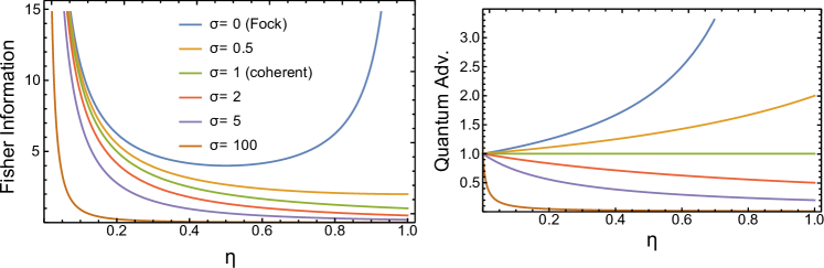
Figure 5: The Fisher information on the parameter $\eta$ per incident photon $\mathcal{F}(\eta)$ (left) and quantum advantage (right) for states with varying Fano factors ($\sigma=\frac{\mathrm{Var}({N}_{0})}{\bar{{N}}_{0}}$). We observe that reducing the $\sigma$ provides an increase in the Fisher information available with that input state.

From Equation 30 one can deduce that for an input photon number distribution of $X({N}_{0})$, the photon number variance of the light after the sample (where the sample transmission coefficient is $\eta$) is given by

$$\mathrm{Var}_{\mathcal{X}_{B}}(N)=\eta^{2}\mathrm{Var}({N}_{0})+(1-\eta)\eta\bar{{N}}_{0},$$ (31)

where $\mathds{E}_{X}[N_{0}]=\bar{{N}}_{0}$ is the mean number of input photons and $\mathrm{Var}({N}_{0})$ is the variance. Using the estimator $\hat{\eta}=N/\bar{N}_{0}$ allows the variance on the estimator to be computed using the relationship for the propagation of errors: $\mathrm{Var}(\hat{\eta})=\left(\frac{\partial\hat{\eta}}{\partial N}\right)^{2}\mathrm{Var}_{\mathcal{X}_{B}}(N)$:

$$\mathrm{Var}(\hat{\eta}) =\frac{\mathrm{Var}(N)_{\mathcal{X}_{B}}}{\bar{{N}}_{0}^{2}}$$

$$=\frac{\eta^{2}\mathrm{Var}({N}_{0})+(1-\eta)\eta\bar{{N}}_{0}}{\bar{{N}}_{0}^{2}}$$

$$=\frac{1}{\bar{{N}}_{0}}\left(\eta^{2}\left(\frac{\mathrm{Var}({N}_{0})}{\bar{{N}}_{0}}\right)+(1-\eta)\eta\right)$$

$$=\frac{1}{\bar{{N}}_{0}}\left(\eta^{2}\sigma+(1-\eta)\eta\right).$$ (32)

From this we find that the Fisher information on the parameter $\eta$ per incident photon is given by

$$\mathcal{F}(\eta)=\frac{1}{\eta^{2}\sigma+(1-\eta)\eta}.$$ (33)

Note, that for the coherent state case ($\sigma=1$), we arrive at the same variance as discussed previously. Also, the Fisher information is maximised for the case where $\sigma=0$, which is true for Fock states. Therefore, we confirm Fock state is an optimal probe state for a linear loss channel, as found previously Adesso et al. (2009); Fujiwara (2004). Figure 5 displays the relationship with the input photon number $\sigma$ value and the Fisher information.

I.4 Supplementary Material D: Multipass Strategies

The general features of absorbance estimation also appear when one investigates how multipass or multi-application strategies change the estimation capabilities for quantum and classical light. For completeness, here we look at the problem of estimating a sample transmission $\epsilon$ but where the experimentalist is either allowed to apply this loss multiple times to the beam (through having many copies of the sample), or is allowed to pass the light through the same sample multiple times (see Figure 6). This type of estimation procedure has been previously studied by Birchall et al. who investigated multipass strategies in lossy phase estimation Birchall et al. (2017) and loss estimation Birchall et al. (2019).

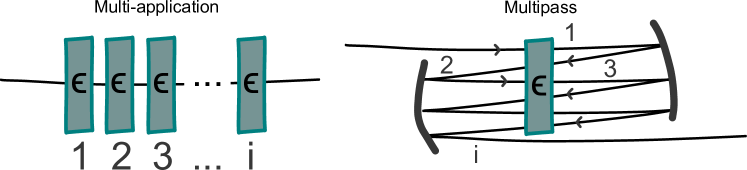
Figure 6: Sketch of practical ways to implement a multi-application (left) or multipass (right) strategy.

Figure 6 demonstrates the two implementations of a multipass or multiapplication strategy. In this case the total transmission of the optical beam is given by

$$\eta=\epsilon^{i},$$ (34)

where $i$ is the number of applications of the sample $\epsilon$ or beam passes, and $\epsilon$ is the single-pass sample transmission. Using the same Fisher information propagation analysis used in the main text, where $\mathcal{F}(\epsilon)=\left(\frac{\partial\eta}{\partial\epsilon}\right)^{2}\mathcal{F}(\eta)$, we find that for a coherent state the Fisher information per incident photon is found to be

$$\mathcal{F}(\epsilon)_{\ket{\alpha}}=\frac{i^{2}}{\epsilon^{2-i}},$$ (35)

and for the Fock state

$$\mathcal{F}(\epsilon)_{\ket{N_{0}}}=\frac{i^{2}}{\epsilon^{2-i}(1-\epsilon^{i})}.$$ (36)

The value of the Fisher information for fixed $\epsilon=0.5$ as a function of applications $i$ is shown in Figure 7.

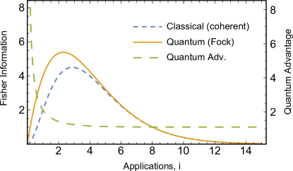
Figure 7: Fisher information per incident photon $\mathcal{F}^{\prime}(\epsilon)$ as a function of the number of passes $i$ for $\epsilon=0.5$. Distribution shows that applying the loss three (two) times in the classical (quantum) case would provide the most precise estimate of $\epsilon$. We note that practically $i$ is limited to discrete values but we have plotted a continuous line to display the simarlarities of this result with that in the main text.

Figure 7 displays very similar behaviour as the Beer-Lambert law absorbance case that was discussed in the main text. In this case, applying the loss sample more that once can increase the precision on the estimate of it’s value. This is similar to increasing the length of the absorbing sample for the absorbance case.

The optimal value of $i$ can be found by finding the location of the maxima of the Fisher information functions in Figure 7 using the same differential approach as the main paper. This produces the value $i^{C}_{optimal}=-\frac{2}{\log{\epsilon}}$ and $i^{Q}_{optimal}=-\frac{W(\frac{2}{e^{2}})-2}{\log{\epsilon}}$ for the classical and quantum cases respectively. The optimal values for the number of passes are shown in Figure 8. This fixes the optimal total absorption $\eta$ to be around 13.5% and 20.3% in the classical and quantum cases respectively (for all values of $\epsilon$).

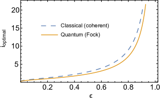
Figure 8: Optimal values of $i$ (number of passes or implementations of the loss $\epsilon$) for maximising $FI^{\prime}(\epsilon)$ for classical and quantum cases.

We see from Figure 7 that the multipass strategy holds many similarities with the Beer-Lambert law case in the main text, where increasing the interaction of the light with the sample can increase the information provided on the loss, even when this results in more total loss being applied to the beam. In this sense, the multipass strategy can be thought of as a discrete version of the Beer-Lambert law (since the number of applications of the sample are limited to integer values).

I.5 Supplementary Material E: Adding Dark Counts to Information Analysis

Results presented in the main text demonstrate deviation of experimental results of the single arm data from what is expected from theoretical predictions. It is hypothesised that this is the result of dark counts from the detectors, which are particularly detrimental for the single arm strategy as the counts from the lossy arm are used in the estimate of the loss. This is not true for the coincidence estimator $\hat{\eta}=N_{signal}/N_{CC}$ where only the singles in the signal channel are considered. Here we look in more detail at the effect of dark counts on the estimation capabilities of a single-arm measurement in a multipass scheme in an effort to reconcile the difference between the theoretical prediction and experimental results.

For a single-arm measurement, estimates of $\eta$ are calculated using the estimator

$$\hat{\eta}=\frac{N_{C}-\bar{N}_{DC}}{\bar{N}_{0}}$$ (37)

where $N_{C}$ is number of detector counts in a sample window, $\bar{N}_{DC}$ is the average number of dark counts over many sample windows, and $\bar{N}_{0}$ is the average number of input photons. The number of counts on the detector is the sum of dark counts in the sample window and the number of incident photons, $N_{i}$, $N_{C}=N_{DC}+N_{i}$. Because of this relationship, and that $N_{i}$ and $N_{DC}$ are independent variables, the variance on $N_{C}$ is just the sum of the individual variances of $N_{i}$ and $N_{DC}$

$$\mathrm{Var}(N_{C})=\mathrm{Var}(N_{i})+\mathrm{Var}(N_{DC}).$$ (38)

Using the standard error propagation formula

$$\mathrm{Var}(\hat{\eta})=\left(\frac{\partial\hat{\eta}}{\partial N_{C}}\right)^{2}\mathrm{Var}(N_{C})$$ (39)

with Equation 37, we find

$$\mathrm{Var}(\hat{\eta})=\frac{\mathrm{Var}(N_{C})}{\bar{N}_{0}^{2}}=\frac{\mathrm{Var}(N_{i})+\mathrm{Var}(N_{DC})}{\bar{N}_{0}^{2}}.$$ (40)

We can relate the detected incident photon number variance with the input (pre-sample) variance using Equation 31

$$\mathrm{Var}(N_{i})=\eta^{2}\mathrm{Var}(N_{0})+(1-\eta)\eta\bar{N}_{0},$$ (41)

which can then be used to give the variance on $\hat{\eta}$ for an arbitrary input states with $\sigma=\mathrm{Var}(N_{0})/\bar{N}_{0}$

$$\mathrm{Var}(\hat{\eta})=\frac{1}{\bar{N}_{0}}\left(\frac{\mathrm{Var}(N_{DC})}{\bar{N}_{0}}+\eta^{2}\sigma+(1-\eta)\eta\right).$$ (42)

This provides an estimator information per incident photon of

$$I(\eta)=\frac{1}{\bar{N}_{0}\mathrm{Var}(\hat{\eta})}=\frac{1}{\frac{\mathrm{Var}(N_{DC})}{\bar{N}_{0}}+\eta^{2}\sigma+(1-\eta)\eta},$$ (43)

which simplifies to the Fisher information bounds for previous scenarios discussed in the main text. We expect this information bound to be optimal (and hence equal to the Fisher information), but have no rigorous proof of this.

I.6 Supplementary Material F: Computing the $\sigma$ Value of a Source

Here we show how to calculate the Fano factor $\sigma$ of a light source from measurement of the noise properties of the light after a channel of transmission $\eta_{l}$. This is useful when trying to estimate the properties of the source when taking measurements with inherent experimental loss. This technique is used in the experimental results of the main paper.

Equation 31 relates the photon number variance after a loss channel to properties of the light before the channel:

$$\mathrm{Var}(N)=\eta_{l}^{2}\mathrm{Var}(N_{0})+(1-\eta_{l})\eta_{l}\bar{N}_{0}.$$ (44)

By dividing by the mean photon number after the channel, $\bar{N}$, we can relate the input sigma value $\sigma_{0}$ to the output one

$$\sigma =\frac{\mathrm{Var}(N)}{\bar{N}}=\frac{\mathrm{Var}(N)}{\eta_{l}\bar{N}_{0}},$$ (45)

$$=\frac{\eta_{l}^{2}\mathrm{Var}(N_{0})}{\eta_{l}\bar{N}_{0}}+\frac{(1-\eta_{l})\eta_{l}\bar{N}_{0}}{\eta_{l}\bar{N}_{0}},$$ (46)

$$=\eta_{l}\sigma_{0}+(1-\eta_{l}),$$ (47)

and therefore

$$\sigma_{0}=\frac{\sigma+\eta_{l}-1}{\eta_{l}}.$$ (48)

Experimentally we measured a Fano factor $\sigma=314.5$ where the channel transmission with no sample present was $\eta_{l}=0.38$. This produces a value of $\sigma_{0}=826$ which is used as the correction factor in the main text.

References

- Truong et al. (2011) G.-W. Truong, E. F. May, T. M. Stace, and A. N. Luiten, Phys. Rev. A 83, 033805 (2011).
- Woutersen et al. (1997) S. Woutersen, U. Emmerichs, and H. J. Bakker, Science 278, 658 (1997).
- Inglese et al. (2007) J. Inglese et al., Nature Chemical Biology 3, 466 (2007).
- Scotter (1990) C. Scotter, Food Control 1, 142 (1990).
- Behera et al. (2012) S. Behera, S. Ghanty, F. Ahmad, S. Santra, and S. Banerjee, J Anal Bioanal Techniques 3, 151 (2012).
- Trumbo et al. (2013) T. A. Trumbo, E. Schultz, M. G. Borland, and M. E. Pugh, Biochemistry and Molecular Biology Education 41, 242 (2013).
- Vontobel et al. (2006) P. Vontobel, E. H. Lehmann, R. Hassanein, and G. Frei, Physica B: Condensed Matter 385-386, 475 (2006).
- Yan et al. (2015) R. Yan, T. J. Edwards, L. M. Pankratz, R. J. Kuhn, J. K. Lanman, J. Liu, and W. Jiang, Journal of structural biology 192, 297 (2015).
- Caves (1981) C. M. Caves, Phys. Rev. D 23, 1693 (1981).
- Ono et al. (2013) T. Ono, R. Okamoto, and S. Takeuchi, Nature Commun. 4, 2426 (2013).
- Sabines-Chesterking et al. (2017) J. Sabines-Chesterking et al., Phys. Rev. Applied 8, 014016 (2017).
- Moreau et al. (2017) P.-A. Moreau et al., Sci. rep. 7, 6256 (2017).
- Zhang et al. (2016) L. Zhang, K. W. C. Chan, and P. K. Verma, Phys. Rev. A 93, 032137 (2016).
- Braginsky (1967) V. B. Braginsky, Zh. Eksp. Teor. Fiz 53, 1434 (1967).
- Aasi et al. (2013) J. Aasi, J. Abadie, B. Abbott, R. Abbott, T. Abbott, M. Abernathy, C. Adams, T. Adams, P. Addesso, R. Adhikari, et al., Nature Photonics 7, 613 (2013).
- Fujiwara (2004) A. Fujiwara, Phys. Rev. A 70, 012317 (2004).
- Adesso et al. (2009) G. Adesso, F. Dell’Anno, S. D. Siena, F. Illuminati, and L. A. M. Souza, Phys. Rev. A 79, 040305 (2009).
- Brida et al. (2010) G. Brida, M. Genovese, and I. R. Berchera, Nature Photonics 4, 227 (2010).
- Whittaker et al. (2017) R. Whittaker et al., New J. Phys. 19, 023013 (2017).
- Lehmann and Casella (2006) E. L. Lehmann and G. Casella, Theory of Point Estimation (Springer Science & Business Media, 2006).
- Paris (2009) M. G. A. Paris, International Journal of Quantum Information 7, 125 (2009).
- (22) See Supplementary Material for a) the derivation of the Fisher information for when experimental loss is present, b) a plot of the quantum advantage as a function of the experimental loss parameter , c) a derivation of the Fisher information for for states with arbitrary Fano factor, d) derivation of the Fisher information for multipass strategies, e) the experimental analysis including dark counts, f) calculation of the Fano factor for the experiment source.
- Corless et al. (1996) R. M. Corless, G. H. Gonnet, D. E. G. Hare, D. J. Jeffrey, and D. E. Knuth, Advances in Computational Mathematics 5, 329 (1996).
- Birchall et al. (2017) P. M. Birchall, J. L. O’Brien, J. C. F. Matthews, and H. Cable, Phys. Rev. A 96, 062109 (2017).
- Birchall et al. (2019) P. M. Birchall, E. J. Allen, T. M. Stace, J. L. O’Brien, J. C. F. Matthews, and H. Cable, arXiv preprint arXiv:1910.00857 (2019).
- Blauensteiner et al. (2009) B. Blauensteiner, I. Herbauts, S. Bettelli, A. Poppe, and H. Hübel, Physical Review A 79, 063846 (2009).
- Burke et al. (1973) R. W. Burke, E. R. Deardorff, and O. Menis, Accuracy in Spectrophotometry and Luminescence Measurements: Proceedings 378, 95 (1973).