Totally Deep Support Vector Machines

Abstract

Support vector machines (SVMs) have been successful in solving many computer vision tasks including image and video category recognition especially for small and mid-scale training problems. The principle of these non-parametric models is to learn hyperplanes that separate data belonging to different classes while maximizing their margins. However, SVMs constrain the learned hyperplanes to lie in the span of support vectors, fixed/taken from training data, and this reduces their representational power and may lead to limited generalization performances.
In this paper, we relax this constraint and allow the support vectors to be learned (instead of being fixed/taken from training data) in order to better fit a given classification task. Our approach, referred to as deep total variation support vector machines, is parametric and relies on a novel deep architecture that learns not only the SVM and the kernel parameters but also the support vectors, resulting into highly effective classifiers. We also show (under a particular setting of the activation functions in this deep architecture) that a large class of kernels and their combinations can be learned. Experiments conducted on the challenging task of skeleton-based action recognition show the outperformance of our deep total variation SVMs w.r.t different baselines as well as the related work.

1 Introduction

Support vector machine (SVM) — also known as support vector network — has been a mainstream standard in machine learning for a while [35, 37, 3, 24, 1, 2, 24, 4, 5, 79, 6, 7, 14, 8, 9, 10, 11, 12, 13, 108, 15, 16] before deep learning has been re-popularized by the seminal work of  [34] and [54, 55, 56, 57, 60, 63, 59, 21]. The general idea of SVMs [28] is to learn hyperplanes that separate populations of training data belonging to different classes while maximizing their margin. These models have been successfully applied to different pattern recognition tasks including image category recognition especially for small or mid-scale training problems (see for instance [99, 40, 51, 41, 42, 43, 27, 44, 45, 46, 58, 47, 48, 49, 62, 50, 85, 52, 65, 53, 64, 79, 30, 97, 85, 27]). However, the success of SVMs is highly dependent on the appropriate choice of kernels. The latter, defined as symmetric positive semi-definite functions, should reserve large values to highly similar content and vice-versa [103, 88]. Existing kernels are either handcrafted (such as gaussian, histogram intersection, etc. [19, 80, 114, 38, 106]) or trained using multiple kernels [73, 74, 76, 77, 78] and explicit kernel maps [66, 67, 75, 68, 70, 69, 71, 72] as well as their deep variants [81, 82, 83, 84, 86, 87, 89, 33].

SVMs are basically non-parametric models; their training consists in solving a constrained quadratic programming (QP) problem [35] whose parameter set grows as the size of training data increases. The solution of a given QP (the separating hyperplane) is defined in the span of a subset of training data known as the support vectors, i.e., as a linear combination of training data whose Lagrange multipliers are strictly positive. Constraining the SVM solution in the span of fixed support vectors contributes in making the QP convex and always convergent to a global solution regardless of its initialization; however, this reduces the representational power of the learned SVMs as only a subclass of possible functions is explored during optimization (i.e., only those defined in the span of fixed support vectors), and this makes the estimation risk of SVMs structurally high compared to other models (including deep learning ones [91]), especially when the support vectors are not sufficiently representative of the actual distribution of training and test data.

In this paper, we introduce an alternative learning algorithm referred to as total variation support vector machine (TV SVM) where the support vectors, kernels and their combinations are all allowed to vary (together with the original SVM parameters) resulting into more flexible and highly discriminant classifiers. Our model is parametric and based on a novel deep network architecture that includes three major steps: (i) support vector learning as a part of individual kernel design, (ii) kernel combination and (iii) SVM parameter learning. We will show, for a particular setting of the activation functions in this deep architecture, that a large class of kernels (including distance and inner product-based as well as their combinations) can be modeled. The non-convexity of the underlying deep learning problem makes the class of possible solutions larger compared to the ones obtained using standard (convex and non-parametric) SVMs. In contrast to the latter, the VC-dimension [29] of our parametric TV SVMs is finite; according to Vapnik’s VC-theory  [31], the finiteness of the VC-dimension avoids loose generalization bounds, reduces the risk of over-fitting and guarantees better performances as also shown in our experiments.

In this proposed framework, the learned support vectors act as kernel parameters and make it possible to map input data to multiple kernel features prior to their classification (as also achieved in [66, 67, 68, 69, 71, 72]). Nevertheless, the proposed framework is conceptually different from these related methods; the latter consider the support vectors fixed/taken from training data in order to design explicit kernel maps prior to learn parametric SVMs while in our method, the support vectors are optimized to better fit the task at hand. Our method is also different from the reduced set technique [36] and the deep kernel nets (for instance [83, 84, 87, 89, 33]). Indeed, the latter operate on precomputed kernel inputs (gram matrices) while the former aims at reducing the complexity of pre-trained nonlinear SVM classifiers using a reduced set of virtual support vectors obtained by minimizing a least squares criterion between the initial and newly generated hyperplane classifiers. Furthermore, the reduced set technique assumes that the initial SVMs are already pre-trained (which could be intractable for large scale problems); besides, the newly generated classifiers could be biased especially when the original pre-trained SVMs are highly complex and nonlinear. Finally, resulting from the parametric setting of our approach, its training and testing complexity is a priori controllable.

The rest of this paper is organized as follows; section 2 reminds the general formulation of SVMs and their deep extensions using kernel networks. Section 3 introduces our main contribution; a total variation SVM that makes it possible to learn not only kernels and SVMs but also the support vectors. Section 4 shows the validity of our method through extensive experiments on the challenging task of skeleton-based action recognition. Section 5 concludes the paper while providing possible extensions for a future work.

2 Deep SVM networks

Define ${\cal X}\subseteq\mathbb{R}^{p}$ as an input space corresponding to all the possible data (e.g., images or videos) and let ${\cal S}=\{\mathbf{x}_{1},\dots,\mathbf{x}_{n},\dots,\mathbf{x}_{n+m}\}$ be a finite subset of $\cal X$ with an arbitrary order. This order is defined so only the first $n$ labels of $\cal S$, denoted $\{{\bf y}_{1},\dots,{\bf y}_{n}\}$, are known (with ${\bf y}_{i}\in\{-1,+1\}$).

2.1 Hinge loss max-margin inference at a glance

Max margin inference aims at building a decision function $f$ that predicts a label ${\bf y}$ for any given input data $\mathbf{x}$; this function is trained on ${\cal L}=\{\mathbf{x}_{1},\dots,\mathbf{x}_{n}\}$ and used in order to infer labels on ${\cal U}={\cal S}\backslash{\cal L}$. In the max-margin classification [29], we consider ${\phi}$ as a mapping of the input data (in $\cal X$) into a high dimensional space $\mathcal{H}$. The dimension of $\cal H$ is usually sufficiently large (possibly infinite) in order to guarantee linear separability of data.

Assuming data linearly separable in $\mathcal{H}$, the hinge loss max-margin learning finds a hyperplane $f$ (with a normal $\mathbf{w}$ and shift $b$) that separates $n$ training samples $\{(\mathbf{x}_{i},{\bf y}_{i})\}_{i=1}^{n}$ while maximizing their margin. The margin is defined as twice the distance between the closest training samples w.r.t $f$ and the optimal $(\hat{\mathbf{w}},\hat{b})$ corresponds to

$$\begin{array}[]{cl}\underset{\mathbf{w},b}{\text{argmin}}&\displaystyle{\frac{1}{2}}\left\|\mathbf{w}\right\|_{2}^{2}+C\sum_{i=1}^{n}\ell({\bf y}_{i},f({\bf x}_{i})),\end{array}$$ (1)

which is the primal form of the max-margin support vector machine, $\|.\|_{2}^{2}$ is the $\ell_{2}$-norm, $C>0$ and $\ell({\bf y}_{i},f({\bf x}_{i}))$ is the hinge loss function defined as $\max(0,1-{\bf y}_{i}f({\bf x}_{i}))$; a differentiable (and also convex) surrogate of this loss is used in practice and defined as $\log(1+\exp(.))$. Given $\mathbf{x}_{i}\in{\cal U}$, the class of $\mathbf{x}_{i}$ in $\{-1,+1\}$ is decided by the sign of $f(\mathbf{x}_{i})={\bf w}^{\prime}{{\phi}(\mathbf{x}_{i})}+b$ with ${\bf w}^{\prime}$ being the transpose of ${\bf w}$. Following the kernel trick and the representer theorem [29], one may write the solution $\bf w$ of the above problem as

$$\begin{array}[]{l}{\bf w}=\displaystyle\sum_{j=1}^{n}\alpha_{j}{\bf y}_{j}\phi(\mathbf{x}_{j}),\end{array}$$ (2)

hence $f(\mathbf{x}_{i})$ can also be expressed as $\sum_{j=1}^{n}\alpha_{j}{\bf y}_{j}\kappa(\mathbf{x}_{i},\mathbf{x}_{j})+b$, where $\alpha=(\alpha_{1}\dots\alpha_{n})^{\prime}$ is a vector of positive real-valued training parameters found as the solution of the following dual problem

$$\begin{array}[]{lll}\displaystyle&\displaystyle\min_{\alpha\geq 0,b}&\displaystyle\frac{1}{2}\sum_{i,j=1}^{n}\alpha_{i}\alpha_{j}{\bf y}_{i}{\bf y}_{j}\kappa(\mathbf{x}_{i},\mathbf{x}_{j})\\ &&\ \ \ \ +C\displaystyle\sum_{i=1}^{n}\ell({\bf y}_{i},\sum_{j=1}^{n}\alpha_{j}{\bf y}_{j}\kappa(\mathbf{x}_{i},\mathbf{x}_{j})+b),\end{array}$$ (3)

here $\kappa(.,.)=\langle{\phi}(.),{\phi}(.)\rangle$ is a symmetric and positive (semi-definite) kernel function [26, 28]. The closed form of $\kappa$ is defined among a collection of existing elementary (a.k.a individual) kernels including linear, gaussian and histogram intersection and the underlying mapping ${\phi}(x)\in{\cal H}$ is usually implicit, i.e., it does exist but it is not necessarily known and may be infinite dimensional. We consider in the remainder of this paper an approach that learns better kernels; the latter are deep and designed in order to i) guarantee linear separability of data in $\cal L$, ii) to ensure better generalization performance using deep networks and iii) to ensure positive definiteness by construction (see subsequent sections and also appendix).

2.2 Deep multiple kernels

We aim to learn an implicit mapping function that recursively characterizes a nonlinear and deep combination of multiple elementary kernels [90]. For each layer $l\in\{2,\dots,L\}$ and its associated unit $p$, a kernel domain $\big{\{}{\kappa}_{p}^{(l)}(\cdot,\cdot)\big{\}}$ is recursively defined as

$${\kappa}_{p}^{l}(\cdot,\cdot)=g\big{(}\sum_{q}{\bf\beta}_{q,p}^{l-1}\ \kappa_{q}^{l-1}(\cdot,\cdot)\big{)},$$ (4)

where $g$ is a nonlinear activation function chosen in order to guarantee the positive semi-definiteness of the learned deep kernels (see more details in appendix). In the above equation, $q\in\{1,\dots,n_{l-1}\}$, $n_{l-1}$ is the number of units in layer $(l-1)$ and $\{{\bf\beta}^{l-1}_{q,p}\}_{q}$ are the (learned) weights associated to kernel ${\kappa}_{p}^{l}$. In particular, $\{{\kappa}_{p}^{1}\}_{p}$ are the input elementary kernels including linear and histogram intersection kernels, etc. When $L=2$, the architecture is shallow, and it is equivalent to the 2-layer MKL of Zhuang et al. [32]. For larger values of $L$, the network becomes deep.

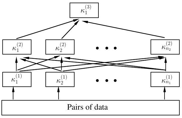
Figure 1: The deep kernel learning architecture with two intermediate layers and an output layer. The input of this network corresponds to different elementary kernels evaluated on a given pair of data.

We notice that the deep kernel network in essence is a multi-layer perceptron (MLP), with nonlinear activation functions (see Fig. 1). The difference is that the last layer is not designed for classification, rather than to deliver a similarity value. However, we can use standard back-propagation algorithm specific for MLP to optimize the weights in the deep kernel network. Considering the output kernel $\kappa_{1}^{L}$ (and its parameters ${\bf\beta}$), a slight variant (denoted as $J(\alpha,{{\bf\beta}})$) of the objective function in Eq. 3 is defined as

$$\begin{array}[]{lll}\displaystyle&\displaystyle\min_{\alpha\geq 0,b,{\bf\beta}}&\displaystyle\frac{1}{2}\sum_{i,j=1}^{n}\alpha_{i}\alpha_{j}{\bf y}_{i}{\bf y}_{j}\kappa_{1}^{L}(\mathbf{x}_{i},\mathbf{x}_{j})\\ \displaystyle&&\ \ \ \ +\displaystyle C\sum_{i=1}^{n}\ell({\bf y}_{i},\sum_{j=1}^{n}\alpha_{j}{\bf y}_{j}\kappa_{1}^{L}(\mathbf{x}_{i},\mathbf{x}_{j})+b)\\ &\textrm{s.t.}&\displaystyle\sum_{q=1}^{n_{l-1}}{\bf\beta}_{q,p}^{l-1}=1,\ \ \ {\bf\beta}_{q,p}^{l-1}\geq 0,\\ &&l\in\{2,\dots,L\},\ \ \ p\in\{1,\dots,n_{l}\}.\end{array}$$ (5)

Note that this objective function is now optimized w.r.t both $\alpha$ and ${\bf\beta}$ (the parameters of the deep multiple kernels). Assuming that the computation of gradients of the objective function $J$ w.r.t the output kernel $\kappa^{(L)}_{1}$ (i.e. $\frac{\partial J}{\partial\kappa^{L}_{1}(.,.)}$) is tractable; according to the chain rule, the corresponding gradients w.r.t coefficients ${\bf\beta}$ are computed, and then used to update these weights using gradient descent (see also extra details in section 3.2). Note also that the above problem is not convex anymore (w.r.t $\alpha$, $\beta$ when taken jointly), however, releasing convexity makes it possible to explore a larger set of possible solutions resulting into a better estimator as also discussed subsequently and also in experiments.

Figure 2: This figure shows the architecture of our deep net including individual and deep kernel evaluations as well as SVM classification. The first layer is fed with the input vector ${\bf x}$ (whose dimension is $D$) which is transferred to different branches; each one corresponds to one individual kernel (linear, polynomial, histogram intersection, etc.). In the second layer, the $\sigma_{1}$ activation is first applied to all the dimensions of ${\bf x}$, then each dimension of the resulting activated signal $\sigma_{1}({\bf x})$ is multiplied, in the third layer, by the $N$ (re-parameterized) weights $\{\sigma_{4}({\cal Z})\}$ (as shown in Eq 9) prior to apply the $\sigma_{2}$ activation; here $N$ corresponds to the number of virtual support vectors in ${\cal Z}$ and these weights (or virtual support vectors) are shared through different branches (i.e., individual kernels). In the fourth layer, the results of the previous one are pooled across dimensions resulting into $N$ kernel values. Note that these $N$ kernel values are activated by $\sigma_{3}()$ and fed to the deep multiple kernel MLP, in the fifth layer, resulting into $N$ deep multiple kernel values which are linearly combined in the last layer for classification (as shown in Eq. 8).

3 Deep total variation SVM networks

Considering the primal form in Eq. 1 (and Eq. 2); for a given $N$ (targeted number of support vectors), we define a more general class of solutions as

$${\bf w}=\sum_{j=1}^{N}\alpha_{j}\phi(\mathbf{z}_{j}).$$ (6)

In the above form, ${\bf w}$ is not written in the span of the fixed training set $\cal L$ but in the span of a more general set ${\cal Z}=\{{\bf z}_{j}\}_{j=1}^{N}\subset\mathbb{R}^{p}$, referred to as virtual support vectors, which varies together with $\{\alpha_{j}\}_{j}$. As the labels of $\cal Z$ are unknown, these labels are implicitly embedded into $\{\alpha_{j}\}_{j}$, so the latter are not constrained to be positive anymore. With this more general setting of ${\bf w}$ (i.e., $\{\alpha_{j}\}_{j}$ and $\{{\bf z}_{j}\}_{j}$), one may define a larger set of possible solutions, and thereby obtain a better universal estimator; at least because the set of solutions defined by Eq. 2 is included in Eq. 6 (while the converse is not true).

Considering this variant of ${\bf w}$, the objective function (5) can be rewritten as

$$\begin{array}[]{lll}\displaystyle&\displaystyle\min_{\alpha,b,{\cal Z},{\bf\beta}}&\displaystyle\frac{1}{2}\sum_{i,j=1}^{N}\alpha_{i}\alpha_{j}\kappa_{1}^{L}({\bf z}_{i},{\bf z}_{j})\\ &&\displaystyle\ \ \ \ +C\sum_{i=1}^{n}\ell({\bf y}_{i},\sum_{j=1}^{N}\alpha_{j}\kappa_{1}^{L}(\mathbf{x}_{i},{\bf z}_{j})+b)\\ &\textrm{s.t.}&\displaystyle\sum_{q=1}^{n_{l-1}}{\bf\beta}_{q,p}^{l-1}=1,\ \ \ {\bf\beta}_{q,p}^{l-1}\geq 0,\\ &&l\in\{2,\dots,L\},\ \ \ p\in\{1,\dots,n_{l}\},\end{array}$$ (7)

and the decision function becomes

$$\begin{array}[]{lll}f({\bf x}_{i})=\displaystyle\sum_{j=1}^{N}\alpha_{j}\kappa_{1}^{L}({\bf x}_{i},{\bf z}_{j})+b.\end{array}$$ (8)

The left-hand side term of the objective function (7) acts as a regularizer (which is now totally independent from the training set $\cal L$) while the right-hand side term still corresponds to the hinge loss. With this new constrained minimization problem all the parameters are allowed to vary including the virtual support vectors $\cal Z$, together with $\alpha$ and $b$ as well as the mixing parameters (in $\beta$) of the deep multiple kernels. In contrast to standard non-parametric SVMs (as well as their multiple kernel variants), this formulation is totally parametric, which means, that the decision function (once trained on a given $\cal L$) is defined using a fixed-length set of trained parameters $\cal Z$, $\beta$, $\alpha$ and $b$. Note that the complexity of evaluating (8) scales linearly w.r.t the size of $\cal S$ while for standard (non-parametric) SVM this complexity is quadratic. As shown in the following section, one may consider a deep net architecture in order to effectively and efficiently train and evaluate the model in Eq. 8. In the remainder of this paper, this model will be referred to as total variation SVM; as shown later in experiments, this model is highly flexible and shows superior performances compared to individual and multi-kernel SVMs as well as their deep variants.

		$k({\bf x},{\bf z})$	$\sigma_{1}(t)$	$\sigma_{2}(t)$	$\sigma_{3}(t)$	$\sigma_{4}(t)$
Inner product based	Linear	$\langle{\bf x},{\bf z}\rangle$	$t$	$t$	$t$	$t$
	Polynomial	$\langle{\bf x},{\bf z}\rangle^{p}$	$t$	$t$	$t^{p}$	$t$
	Sigmoid	$\frac{1}{1+\exp(-\beta\langle{\bf x},{\bf z}\rangle)}$	$t$	$t$	$\frac{1}{1+\exp(-\beta t)}$	$t$
	tanh	$\tanh(a\langle{\bf x},{\bf z}\rangle+b$)	$t$	$t$	$\tanh(at+b)$	$t$
Distance based	Gaussian	$\exp(-\beta\|{\bf x}-{\bf z}\|^{2})$	$\exp(t)$	$\log(t)^{2}$	$\exp(-\beta t)$	$\exp(-t)$
	Laplacian	$\exp(-\beta\|{\bf x}-{\bf z}\|)$	$\exp(t)$	$\log(t)^{2}$	$\exp(-\beta\sqrt{t})$	$\exp(-t)$
	Power	$-\|{\bf x}-{\bf z}\|^{p}$	$\exp(t)$	$\log(t)^{2}$	$-t^{p/2}$	$\exp(-t)$
	Multi-quadratic	$\sqrt{\|{\bf x}-{\bf z}\|^{2}+b^{2}}$	$\exp(t)$	$\log(t)^{2}$	$\sqrt{t+b^{2}}$	$\exp(-t)$
	Inverse Multi-quadratic	$\frac{1}{\sqrt{\|{\bf x}-{\bf z}\|^{2}+b^{2}}}$	$\exp(t)$	$\log(t)^{2}$	$\frac{1}{\sqrt{t+b^{2}}}$	$\exp(-t)$
	Log	$-\log(\|{\bf x}-{\bf z}\|^{p}+1)$	$\exp(t)$	$\log(t)^{2}$	$-\log(t^{p/2}+1)$	$\exp(-t)$
	Cauchy	$\frac{1}{1+\frac{\|{\bf x}-{\bf z}\|^{2}}{\sigma^{2}}}$	$\exp(t)$	$\log(t)^{2}$	$\frac{1}{1+\frac{t}{\sigma^{2}}}$	$\exp(-t)$
	Histogram intersection	$\sum_{d}\min({\bf x}_{.,d},{\bf z}_{.,d})$	$\exp(\exp(-\beta(1-t)))$	$\frac{1}{\beta}\log(\log(t))+1$	$t$	$\sigma_{1}(t)$

TABLE I: This table shows the setting of $\sigma_{1}$, $\sigma_{2}$, $\sigma_{3}$, $\sigma_{4}$ for different kernel functions. Note that the best parameters of these individual kernels are set using cross validation.

3.1 Neural consistency and architecture design

In contrast to decision functions defined with the primal parameters $\bf w$, the one in Eq. 8 cannot be straightforwardly evaluated using standard neural units as input kernels $\{\kappa_{q}^{1}\}$ in Eq. 4 may have general forms. Hence, modeling Eq. 8 requires a careful design; our goal in this paper, is not to change the definition of neural units, but instead to adapt Eq. 8 in order to make it consistent with the usual definition of neural units. In what follows, we introduce the overall architecture associated to the decision function $f(.)$ (and also $\kappa_{1}^{L}$) for different input kernels $\{\kappa_{q}^{1}\}_{q}$ including linear, polynomial, gaussian and histogram intersection as well as a more general class of kernels (see for instance [18, 23]).

Definition 1 (Neural consistency)

Let ${\bf x}_{.,d}$ (resp. ${\bf z}_{.,d}$) denote the $d^{th}$ dimension of a vector ${\bf x}$ (resp. ${\bf z}$). For a given (fixed or learned) ${\bf z}$, a kernel $\kappa$ is referred to as “neural-consistent” if

$$\kappa({\bf x},{\bf z})=\sigma_{3}\big{(}\sum_{d}\sigma_{2}(\sigma_{1}({\bf x}_{.,d}).\omega_{d})\big{)},$$ (9)

with $\omega_{d}=\sigma_{4}({\bf z}_{.,d})$ and being $\sigma_{1}$, $\sigma_{2}$, $\sigma_{3}$, $\sigma_{4}$ any arbitrary real-valued activation functions.

Considering the above definition, it is easy to see that deep kernels defined in Eq. 4 are neural consistent provided that their input kernels are also neural consistent; the latter include (i) the linear $\langle{\bf x},{\bf z}\rangle$, (ii) the polynomial $\langle{\bf x},{\bf z}\rangle^{p}$, (iii) the hyperbolic tangent $\tanh\langle{\bf x},{\bf z}\rangle$, (iv) the gaussian $\exp(-\beta\|{\bf x}-{\bf z}\|^{2})$ and (v) the histogram intersection $\sum_{d}\min({\bf x}_{.,d},{\bf z}_{.,d})$. Neural consistency is straightforward for inner product-based kernels (namely linear, polynomial and tanh) while for shift invariant kernels such as the gaussian, one may write $\exp(-\beta\|{\bf x}-{\bf z}\|_{2}^{2})=\sigma_{3}\big{(}\sum_{d}\sigma_{2}(\sigma_{1}({\bf x}_{.,d}).\omega_{d})\big{)}$ with $\sigma_{1}(.)=\exp(.)$, $\sigma_{2}(.)=\log(.)^{2}$, $\sigma_{3}(.)=\exp(-\beta(.))$ and $\omega_{d}=\exp(-{\bf z}_{.,d})$. For histogram intersection, it is easy to see that $\sum_{d}\min({\bf x}_{.,d},{\bf z}_{.,d})=\sum_{d}1-\max(1-{\bf x}_{.,d},1-{\bf z}_{.,d})$ and one may obtain (for a sufficiently large $\beta$) $\sum_{d}1-\max(1-{\bf x}_{.,d},1-{\bf z}_{.,d})\approx\sigma_{3}\big{(}\sum_{d}\sigma_{2}(\sigma_{1}({\bf x}_{.,d}).\omega_{d})\big{)}$ using $\sigma_{1}(.)=\exp(\exp(-\beta(1-(.))))$, $\sigma_{2}(.)=\frac{1}{\beta}\log(\log(.))+1$, $\sigma_{3}(.)=(.)$ and $\omega_{d}=\sigma_{1}({\bf z}_{.,d})$.
Following the above example, neural consistent kernels (including linear, polynomial, gaussian, histogram intersection) can be expressed using the deep net architecture shown in Fig. 2. Neural consistency can be extended to other shift invariant kernels including: multi-quadratic, inverse multi-quadratic, power, log, Cauchy, Laplacian, etc. (see for instance [19] for a taxonomy of the widely used functions in kernel machines; see also table I for the setting of $\sigma_{1}$, $\sigma_{2}$, $\sigma_{3}$, $\sigma_{4}$ for different kernels).

Figure 3: This figure shows the whole keypoint tracking and description process on the motion stream.

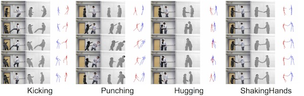
Figure 4: This figure shows a sample of videos and skeletons associated to different action categories taken from the SBU dataset;
see https://www3.cs.stonybrook.edu/$\sim$kyun/research/kinect_interaction/index.html.

3.2 Optimization

All the parameters of the network (including the virtual support vectors, the mixing parameters of the multiple kernels and the weights of the SVMs) are learned end-to-end using back-propagation and stochastic gradient descent. However, as the mixing parameters $\beta$ are constrained, we consider a slight variant in order to implement these constraints.
From proposition 2 (see appendix), provided that i) the input kernels are conditionally positive definite (c.p.d), ii) the activation function $g$ preserves the c.p.d (as leaky-ReLU) and iii) the weights $\{{\bf\beta}_{q,p}^{l-1}\}$ (written for short as $\{{\bf\beta}_{q,p}^{l}\}$ in the remainder of this section) are positive, all the resulting multiple kernels in Eq. 4 will also be c.p.d and admit equivalent positive definite kernels (following proposition 1 in appendix), and thereby max-margin SVM can be achieved. Note that conditions (i) and (ii) are satisfied by construction while condition (iii) requires adding equality and inequality constraints to Eq. 4, i.e., ${\bf\beta}_{q,p}^{l}\in[0,1]$ and $\sum_{q}{\bf\beta}_{q,p}^{l}=1$. In order to implement these constraints, we consider a re-parametrization in Eq. 4 as ${\bf\beta}_{q,p}^{l}=h({\hat{{\bf\beta}}}_{q,p}^{l})/{\sum_{q}h({\hat{{\bf\beta}}}_{q,p}^{l})}$ for some $\{\hat{{\bf\beta}}_{q,p}^{l}\}$ with $h$ being strictly monotonic real-valued (positive) function and this allows free settings of the parameters $\{\hat{{\bf\beta}}_{q,p}^{l}\}$ during optimization while guaranteeing ${\bf\beta}_{q,p}^{l}\in[0,1]$ and $\sum_{q}{\bf\beta}_{q,p}^{l}=1$. During back-propagation, the gradient of the loss $J$ (now w.r.t ${\hat{{\bf\beta}}}$’s) is updated using the chain rule as

$$\begin{array}[]{lll}\displaystyle\frac{\partial J}{\partial{\hat{{\bf\beta}}}_{q,p}^{\l}}&=&\displaystyle\frac{\partial J}{\partial{\bf\beta}_{q,p}^{l}}.\frac{\partial{\bf\beta}_{q,p}^{l}}{\partial{\hat{{\bf\beta}}}_{q,p}^{l}}\\ \ \ \ \ \textrm{with}&&\ \ \ \displaystyle\frac{\partial{\bf\beta}_{q,p}^{l}}{\partial{\hat{{\bf\beta}}}_{q,p}^{\l}}=\displaystyle\frac{h^{\prime}({\hat{{\bf\beta}}}_{q,p}^{l})h(\sum_{r\neq q}{\hat{{\bf\beta}}}_{r,p}^{l})}{(h({\hat{{\bf\beta}}}_{q,p}^{l})+h(\sum_{r\neq q}{\hat{{\bf\beta}}}_{r,p}^{l}))^{2}},\end{array}$$ (10)

in practice $h(.)=\exp(.)$ and $\frac{\partial J}{\partial{\bf\beta}_{q,p}^{l}}$ is obtained from layerwise gradient backpropagation (as already integrated in standard deep learning tools including PyTorch and TensorFlow). Hence, $\frac{\partial J}{\partial{\hat{{\bf\beta}}}_{q,p}^{l}}$ is obtained by multiplying the original gradient $\frac{\partial J}{\partial{{\bf\beta}}_{q,p}^{l}}$ by $\frac{\exp(\sum_{r}{\hat{{\bf\beta}}}_{r,p}^{l})}{(\exp({\hat{{\bf\beta}}}_{q,p}^{l})+\exp(\sum_{r\neq q}{\hat{{\bf\beta}}}_{r,p}^{l}))^{2}}$.

4 Experiments

We evaluate the performance of our total variation SVM on the challenging task of action recognition, using the SBU kinect dataset [93]. The latter is an interaction dataset acquired using the Microsoft kinect sensor; it includes in total 282 video sequences belonging to 8 categories: “approaching”, “departing”, “pushing”, “kicking”, “punching”, “exchanging objects”, “hugging”, and “hand shaking” with variable duration, viewpoint changes and interacting individuals (see examples in Fig. 4). In all these experiments, we use the same evaluation protocol as the one suggested in [93] (i.e., train-test split) and we report the average accuracy over all the classes of actions.

	Standard SVM with SVs	Total variation SVM w.r.t different # of learned SVs
	fixed/taken from the training set	10	50	100	150	200	250
Linear	81.5385	90.7692	92.3077	92.3077	93.8462	89.2308	92.3077
Polynomial	84.6154	89.2308	92.3077	92.3077	90.7692	90.7692	90.7692
Sigmoid	83.0769	92.3077	90.7692	92.3077	92.3077	92.3077	92.3077
tanh	83.0769	92.3077	93.8462	90.7692	92.3077	93.8462	93.8462
Gaussian	86.1538	90.7692	92.3077	92.3077	92.3077	92.3077	92.3077
Laplacian	84.6154	83.0769	80.0000	81.5385	87.6923	92.3077	86.1538
Power	86.1538	81.5385	92.3077	93.8462	95.3846	95.3846	95.3846
Multi-quadratic	86.1538	81.5385	90.7692	93.8462	95.3846	93.8462	95.3846
Inverse Multi-quadratic	83.0769	90.7692	93.8462	93.8462	93.8462	93.8462	93.8462
Log	87.6923	78.4615	89.2308	92.3077	93.8462	95.3846	95.3846
Cauchy	86.1538	92.3077	93.8462	93.8462	93.8462	93.8462	93.8462
Histogram Intersection	86.1538	92.3077	92.3077	93.8462	93.8462	93.8462	95.3846
MKL (one layer)	89.2308	80.0000	95.3846	93.8462	95.3846	93.8462	93.8462
MKL (two layers)	87.6923	90.7692	95.3846	93.8462	96.9231	95.3846	95.3846
MKL (three layers)	89.2308	93.8462	95.3846	95.3846	93.8462	95.3846	95.3846

TABLE II: This table shows a comparison of our TV SVM against standard SVM with different individual and multiple kernels.

4.1 Video skeleton description

Given a video ${\cal V}$ in SBU as a sequence of skeletons, each keypoint in these skeletons defines a labeled trajectory through successive frames (see Fig. 3). Considering a finite collection of trajectories $\{v_{i}\}_{i}$ in ${\cal V}$, we process each trajectory using temporal chunking: first we split the total duration of a video into $M$ equally-sized temporal chunks ($M=4$ in practice), then we assign the keypoint coordinates of a given trajectory $v_{i}$ to the $M$ chunks (depending on their time stamps) prior to concatenate the averages of these chunks and this produces the description of $v_{i}$ denoted as $\psi(v_{i})$ and the final description of a given video ${\cal V}$ is $(\psi(v_{1})\ \psi(v_{2})\dots)$ following the same order through trajectories. Hence, two trajectories $v_{i}$ and $v_{j}$, with similar keypoint coordinates but arranged differently in time, will be considered as very different. Note that beside being compact and discriminant, this temporal chunking gathers advantages – while discarding drawbacks – of two widely used families of techniques mainly global averaging techniques (invariant but less discriminant) and frame resampling techniques (discriminant but less invariant). Put differently, temporal chunking produces discriminant descriptions that preserve the temporal structure of trajectories while being frame-rate and duration agnostic.

4.2 Performances and comparison

We trained our TV SVM for 1000 epochs with a batch size equal to $50$ and we set the learning rate (denoted $\nu$) iteratively inversely proportional to the speed of change of the objective function in Eq. 7; when this speed increases (resp. decreases), $\nu$ decreases as $\nu\leftarrow\nu\times 0.99$ (resp. increases as $\nu\leftarrow\nu/0.99$). All these experiments are run on a GeForce GTX 1070 GPU device (with 8 GB memory) and no data augmentation is achieved. Table II shows a comparison of action recognition performances, using TV SVM against different baselines involving individual kernels with support vectors (SVs) fixed/taken from the training set. We also show the results using deep multiple kernel learning (MKL).

From all these results, we observe a clear and a consistent gain of TV SVM w.r.t all the individual kernel settings and their MKL combinations; this gain is further amplified when using deep MKL with only two layers. However, these performances stabilize as the depth of MKL increases since the size of the training set is limited compared to the large number of training parameters in its underlying MLP. These performances also improve quickly as the number of learned (virtual) support vectors $N$ increases, and this results from the flexibility of TV SVM which learns — with few virtual support vectors — relevant representatives of training and test data. These performances consistently improve for all the individual kernels (as well as their MKL combinations) and this is again explained by the modeling capacity of TV SVM. Indeed, the latter captures better the actual decision boundary while standard SVM (even when combined with MKL) is clearly limited when the fixed support vectors are biased (i.e., not sufficiently representative of the actual distribution of the data especially on small or mid-scale problems); hence, learning the MKL+SVM parameters (with fixed SVs) is not enough in order to recover from this bias. In sum, the gain of TV SVM results from the complementary aspects of the used individual kernels and also the modeling capacity of SVMs when the support vectors are allowed to vary.

Finally, we compare the classification performances of our TV SVM against other related methods in action recognition (on SBU) ranging from sequence based such as LSTM and GRU [101, 102, 98] to deep graph (no-vectorial) methods based on spatial and spectral convolution [96, 95, 94]. From the results in table III, TV SVM brings a substantial gain w.r.t state of the art methods, and provides comparable results with the best vectorial methods on SBU (see also [112]).

Perfs 90.00 96.00 94.00 96.00 49.7 80.3 86.9 83.9 80.35 90.41 93.3 90.5 91.51 94.9 97.2 95.7 93.7 96.92 Methods GCNConv [96] ArmaConv [105] SGCConv [95] ChebyNet [94] Raw coordinates [93] Joint features [93] Interact Pose [107] CHARM [109] HBRNN-L [110] Co-occurence LSTM [111] ST-LSTM [113] Topological pose ordering[115] STA-LSTM [98] GCA-LSTM [102] VA-LSTM [104] DeepGRU [101] Riemannian manifold trajectory[100] Our best TV SVM

TABLE III: Comparison against state of the art methods.

5 Conclusion

We introduced in this paper a novel deep total variation support vector machine that learns highly effective classifiers. The strength of our method resides in its ability to models different kernels and to learn their support vectors resulting into better classification performances. Experiments conducted on the challenging action recognition task show the outperformance of this parametric SVM formulation against different baselines including non-parametric SVMs as well as the related work. As a future work, we are currently investigating the application of our method to other computer vision and pattern recognition tasks in order to further study the impact of this highly flexible model.

Appendix

We consider, as $g$ in Eq. (4), the leaky ReLU [20, 22] activation function: leaky ReLU allows learning conditionally positive definite (c.p.d) kernels. In what follows, we discuss the sufficient conditions about the choices of the input kernels, the parameters $\{{\bf\beta}_{q,p}^{l-1}\}$ and the activation function that guarantee this c.p.d property.

Definition 2 (c.p.d kernels)

A kernel $\kappa$ is c.p.d, iff $\forall{\bf x}_{1},\dots,{\bf x}_{n}\in\mathbb{R}^{p}$, $\forall c_{1},\dots,c_{n}\in\mathbb{R}$ (with $\sum_{i=1}^{n}c_{i}=0$), we have $\sum_{i,j}c_{i}c_{j}\kappa({\bf x}_{i},{\bf x}_{j})\geq 0$.

From the above definition, it is clear that any p.d kernel is also c.p.d, but the converse is not true; this property is a weaker (but sufficient) condition in order to learn max margin SVMs (see for instance [28]; see also the following proposition).

Proposition 1 (Berg et al.[17])

Consider $\kappa$ and define $\hat{\kappa}$ with

$$\hat{\kappa}({\bf x}_{i},{\bf x}_{j}) = {\kappa}({\bf x}_{i},{\bf x}_{j})-{\kappa}({\bf x}_{i},{\bf x}_{n+1})$$

$$-{\kappa}({\bf x}_{n+1},{\bf x}_{j})+{\kappa}({\bf x}_{n+1},{\bf x}_{n+1})$$

Then, $\hat{\kappa}$ is positive definite if and only if ${\kappa}$ is c.p.d.

Proof 1

See Berg et al.[17]. Now we derive our main result

Proposition 2

Provided that the input kernels $\{\kappa_{q}^{(1)}\}_{q}$ are c.p.d, and $\{{\bf\beta}_{q,p}^{l-1}\}_{p,q,l}$ belong to the positive orthant of the parameter space; any combination defined as $g(\sum_{q}{{\bf\beta}}_{q,p}^{l-1}\ \kappa_{q}^{l-1})$ with $g$ equal to leaky ReLU is also c.p.d.

Proof 2

Details of the first part of the proof, based on recursion, are omitted and result from the application of definition (2) to $\kappa=\sum_{q}{\bf\beta}_{q,p}^{l-1}\ \kappa_{q}^{l-1}$ (for different values of $l$) while considering $\{\kappa_{q}^{1}\}_{q}$ c.p.d. Now we show the second part of the proof (i.e., if $\kappa$ is c.p.d, then $g(\kappa)$ is also c.p.d for leaky ReLU).
For leaky ReLU, one may write $g(\kappa)=\log(\exp(a\kappa)+\exp(\kappa))$ with $0<a\ll 1$. Considering $\kappa$ c.p.d, and following proposition (1), one may define a positive definite $\hat{\kappa}$ and obtain $\forall\{c_{i}\}_{i}$, $\forall\{{\bf x}_{i}\}_{i}$, $\sum_{i,j=1}^{n}c_{i}c_{j}\exp(\kappa({\bf x}_{i},{\bf x}_{j}))=(*)$ with

$$(*) = \exp(\kappa({\bf x}_{n+1},{\bf x}_{n+1}))$$

$$.\sum_{i,j=1}^{n}(c_{i}\exp(\kappa({\bf x}_{i},{\bf x}_{n+1}))).(c_{j}\exp(\kappa({\bf x}_{n+1},{\bf x}_{j})))$$

$$\ \ \ \ \ \ \ \ \ \ \ \ .\exp(\hat{\kappa}({\bf x}_{i},{\bf x}_{j}))$$

$$\geq 0,$$

so $\exp(\kappa)$ is also positive definite. One may also rewrite $g$ as

$$g(\kappa)=a\ \kappa+\log(1+\exp((1-a)\ \kappa)).$$ (11)

Since $\exp(\kappa)$ is positive definite, it follows that $(1+\exp((1-a)\ \kappa))^{\alpha}$ is also positive definite for any arbitrary $\alpha>0$ and $0<a\ll 1$ so from [25], $\log(1+\exp((1-a)\ \kappa))$ is c.p.d and so is $g(\kappa)$; the latter results from the closure of the c.p.d with respect to the sum.

$\blacksquare$

References

- [1] Weston, Jason, and Chris Watkins. Multi-class support vector machines. Technical Report CSD-TR-98-04, Department of Computer Science, Royal Holloway, University of London, May, 1998.
- [2] Hearst, Marti A., et al. ”Support vector machines.” IEEE Intelligent Systems and their applications 13.4 (1998): 18-28.
- [3] H. Sahbi, X. Li. Context-based support vector machines for interconnected image annotation. Asian Conference on Computer Vision. Springer, Berlin, Heidelberg, 2010.
- [4] Zeng, Zhi-Qiang, et al. ”Fast training support vector machines using parallel sequential minimal optimization.” 2008 3rd international conference on intelligent system and knowledge engineering. Vol. 1. IEEE, 2008.
- [5] Osuna, Edgar, Robert Freund, and Federico Girosi. ”Training support vector machines: an application to face detection.” Proceedings of IEEE computer society conference on computer vision and pattern recognition. IEEE, 1997.
- [6] M. Jiu, H. Sahbi. Laplacian deep kernel learning for image annotation. IEEE International Conference on Acoustics, Speech and Signal Processing, 2016.
- [7] AK, Suykens Johan. Least squares support vector machines. World Scientific, 2002.
- [8] M. Jiu, H. Sahbi. Semi supervised deep kernel design for image annotation. IEEE International Conference on Acoustics, Speech and Signal Processing, 2015 .
- [9] Muller, K-R., et al. ”Predicting time series with support vector machines.” International Conference on Artificial Neural Networks. Springer, Berlin, Heidelberg, 1997.
- [10] Andrews, Stuart, Ioannis Tsochantaridis, and Thomas Hofmann. ”Support vector machines for multiple-instance learning.” Advances in neural information processing systems. 2003.
- [11] M. Jiu, H. Sahbi. Deep representation design from deep kernel networks. Pattern Recognition 88, 447-457, 2019.
- [12] Campbell, William M., Douglas E. Sturim, and Douglas A. Reynolds. ”Support vector machines using GMM supervectors for speaker verification.” IEEE signal processing letters 13.5 (2006): 308-311.
- [13] Platt, John. ”Probabilistic outputs for support vector machines and comparisons to regularized likelihood methods.” Advances in large margin classifiers 10.3 (1999): 61-74.
- [14] H. Sahbi. Coarse-to-fine support vector machines for hierarchical face detection. PhD thesis, Versailles University, 2003.
- [15] Mangasarian, Olvi L., and David R. Musicant. ”Lagrangian support vector machines.” Journal of Machine Learning Research 1.Mar (2001): 161-177.
- [16] Ghaddar, Bissan, and Joe Naoum-Sawaya. ”High dimensional data classification and feature selection using support vector machines.” European Journal of Operational Research 265.3 (2018): 993-1004.
- [17] C. Berg, J. P. R. Christensen, and P. Ressel. Harmonic analysis on semigroups: theory of positive definite and related functions, volume 100. Springer, 1984.
- [18] C. Cortes, M. Mohri, and A. Rostamizadeh. Learning non-linear combinations of kernels. In Advances in neural information processing systems, pages 396–404, 2009.
- [19] M. G. Genton. Classes of kernels for machine learning: a statistics perspective. Journal of machine learning research, 2(Dec):299–312, 2001.
- [20] X. Glorot, A. Bordes, and Y. Bengio. Deep sparse rectifier neural networks. In Proceedings of the fourteenth international conference on artificial intelligence and statistics, pages 315–323, 2011.
- [21] T. Postadjian, A. Le Bris, H. Sahbi, C. Mallet. Investigating the potential of deep neural networks for large-scale classification of very high resolution satellite images. ISPRS Annals 4, 183-190, 2017.
- [22] K. He, X. Zhang, S. Ren, and J. Sun. Delving deep into rectifiers: Surpassing human-level performance on imagenet classification. In Proceedings of the IEEE international conference on computer vision, pages 1026–1034, 2015.
- [23] S. Maji, A. C. Berg, and J. Malik. Efficient classification for additive kernel svms. IEEE transactions on pattern analysis and machine intelligence, 35(1):66–77, 2012.
- [24] F. Yuan, G-S. Xia, H. Sahbi, V. Prinet. Mid-level Features and Spatio-Temporal Context for Activity Recognition. Pattern Recognition. volume 45, number 12, 4182-4191, 2012
- [25] I. J. Schoenberg. Metric spaces and positive definite functions. Transactions of the American Mathematical Society, 44(3):522–536, 1938.
- [26] B. Schölkopf and A. Smola. Learning with Kernels: Support Vector Machines, Regularization, Optimization, and Beyond. The MIT Press, Dec. 2001.
- [27] S. Tollari, P. Mulhem, M. Ferecatu, H. Glotin, M. Detyniecki, P. Gallinari, H. Sahbi, Z-Q. Zhao. A comparative study of diversity methods for hybrid text and image retrieval approaches. In Workshop of the Cross-Language Evaluation Forum for European Languages, pp. 585-592. Springer, Berlin, Heidelberg, 2008.
- [28] J. Shawe-Taylor and N. Cristianini. Kernel methods for pattern analysis. Cambriage University Press, 2004.
- [29] V. Vapnik. Statistical Learning Theory. Wiley, New York, 1998.
- [30] H. Sahbi. CNRS-TELECOM ParisTech at ImageCLEF 2013 Scalable Concept Image Annotation Task: Winning Annotations with Context Dependent SVMs. CLEF (Working Notes). 2013.
- [31] V. Vapnik and A. Sterin. On structural risk minimization or overall risk in a problem of pattern recognition. Automation and Remote Control, 10(3):1495–1503, 1977.
- [32] J. Zhuang, I. Tsang, and S. Hoi. Two-layer multiple kernel learning. In ICML, pages 909–917, 2011.
- [33] M. Jiu and H. Sahbi. Deep kernel map networks for image annotation. IEEE International Conference on Acoustics, Speech and Signal Processing (ICASSP), 2016.
- [34] A. Krizhevsky, I. Sutskever, and G. E. Hinton. Imagenet classification with deep convolutional neural networks. In Advances in neural information processing systems, pages 1097–1105, 2012.
- [35] C. J. Burges. A tutorial on support vector machines for pattern recognition. Data mining and knowledge discovery, 2(2):121–167, 1998.
- [36] C. J. Burges and B. Schölkopf. Improving the accuracy and speed of support vector machines. In Advances in neural information processing systems, pages 375–381, 1997.
- [37] C.-C. Chang and C.-J. Lin. Libsvm: a library for support vector machines. ACM transactions on intelligent systems and technology (TIST), 2(3):27, 2011.
- [38] L. Wang, H. Sahbi. Directed Acyclic Graph Kernels for Action Recognition. Proceedings of the IEEE International Conference on Computer Vision. 2013.
- [39] Xiao, Huang, et al. ”Support vector machines under adversarial label contamination.” Neurocomputing 160 (2015): 53-62.
- [40] Tang, Yichuan. ”Deep learning using linear support vector machines.” arXiv preprint arXiv:1306.0239 (2013).
- [41] Joachims, Thorsten. ”Transductive inference for text classification using support vector machines.” Icml. Vol. 99. 1999.
- [42] A. Mazari, H. Sahbi. Deep Temporal Pyramid Design for Action Recognition. In international Conference on Acoustics, Speech and Signal Processing (ICASSP), 2019
- [43] Guo, Guodong, Stan Z. Li, and Kapluk Chan. ”Face recognition by support vector machines.” Proceedings fourth IEEE international conference on automatic face and gesture recognition (cat. no. PR00580). IEEE, 2000.
- [44] Lilleberg, Joseph, Yun Zhu, and Yanqing Zhang. ”Support vector machines and word2vec for text classification with semantic features.” 2015 IEEE 14th International Conference on Cognitive Informatics and Cognitive Computing (ICCI* CC). IEEE, 2015.
- [45] Q. Oliveau, H. Sahbi. Learning attribute representations for remote sensing ship category classification. IEEE Journal of Selected Topics in Applied Earth Observations and Remote Sensing, 2017.
- [46] Zhang, Shunli, et al. ”Object tracking with multi-view support vector machines.” IEEE Transactions on Multimedia 17.3 (2015): 265-278.
- [47] Chapelle, Olivier, Patrick Haffner, and Vladimir N. Vapnik. ”Support vector machines for histogram-based image classification.” IEEE transactions on Neural Networks 10.5 (1999): 1055-1064.
- [48] H. Sahbi. Coarse-to-fine deep kernel networks. Proceedings of the IEEE International Conference on Computer Vision, 1131-1139, 2017.
- [49] Mountrakis, Giorgos, Jungho Im, and Caesar Ogole. ”Support vector machines in remote sensing: A review.” ISPRS Journal of Photogrammetry and Remote Sensing 66.3 (2011): 247-259.
- [50] Guyon, Isabelle, et al. ”Gene selection for cancer classification using support vector machines.” Machine learning 46.1-3 (2002): 389-422.Joachims, Thorsten. ”Text categorization with support vector machines: Learning with many relevant features.” European conference on machine learning. Springer, Berlin, Heidelberg, 1998.
- [51] H. Sahbi, JY. Audibert, J. Rabarisoa, R. Keriven. Object recognition and retrieval by context dependent similarity kernels. International Workshop on Content-Based Multimedia Indexing, 216-223, 2008.
- [52] Pontil, Massimiliano, and Alessandro Verri. ”Support vector machines for 3D object recognition.” IEEE transactions on pattern analysis and machine intelligence 20.6 (1998): 637-646.
- [53] M. Everingham, L. Van Gool, C. K. Williams, J. Winn, A. Zisserman. The pascal visual object classes (voc) challenge. International journal of computer vision, 88(2), 303-338, 2010.
- [54] L. Deng, D. Yu, et al. Deep learning: methods and applications. Foundations and Trends® in Signal Processing, 7(3–4):197–387, 2014.
- [55] R. Girshick, J. Donahue, T. Darrell, and J. Malik. Rich feature hierarchies for accurate object detection and semantic segmentation. In Proceedings of the IEEE CVPR, pages 580–587, 2014.
- [56] I. Goodfellow, Y. Bengio, and A. Courville. Deep Learning. MIT Press, 2016.
- [57] K. He, X. Zhang, S. Ren, and J. Sun. Deep residual learning for image recognition. In Proceedings of the IEEE conference on computer vision and pattern recognition, pages 770–778, 2016.
- [58] N Boujemaa, F Fleuret, V Gouet, H Sahbi. Visual content extraction for automatic semantic annotation of video news. The proceedings of the SPIE Conference, San Jose, CA 6, 2004.
- [59] O. Russakovsky, J. Deng, H. Su, J. Krause, S. Satheesh, S. Ma, Z. Huang, A. Karpathy, A. Khosla, M. Bernstein, et al. Imagenet large scale visual recognition challenge. International Journal of Computer Vision, 115(3):211–252, 2015.
- [60] R. K. Srivastava, K. Greff, and J. Schmidhuber. Training very deep networks. In Advances in neural information processing systems, pages 2377–2385, 2015.
- [61] Y. Taigman, M. Yang, M. Ranzato, and L. Wolf. Deepface: Closing the gap to human-level performance in face verification. In Proceedings of the IEEE conference on computer vision and pattern recognition, pages 1701–1708, 2014.
- [62] N. Bourdis, D. Marraud, H. Sahbi. Constrained optical flow for aerial image change detection. IEEE International Geoscience and Remote Sensing Symposium, 4176-4179, 2011.
- [63] C. Szegedy, W. Liu, Y. Jia, P. Sermanet, S. Reed, D. Anguelov, D. Erhan, V. Vanhoucke, and A. Rabinovich. Going deeper with convolutions. In Proceedings of the IEEE conference on computer vision and pattern recognition, pages 1–9, 2015.
- [64] M. Villegas, R. Paredes, B. Thomee, Overview of the imageclef 2013 scalable concept image annotation subtask, in: CLEF 2013 Evaluation Labs and Workshop, 2013.
- [65] H. Sahbi. Scene Decoding with Finite State Machines. 25th IEEE International Conference on Image Processing (ICIP), 485-489, 2018.
- [66] A. Rahimi, B. Recht, Random features for large-scale kernel machines, in: Advances in Neural Information Processing Systems (NIPS), Vol. 20, 2007, pp. 1177–1184.
- [67] F. Li, C. Ionescu, C. Sminchisescu, Random fourier approximations for skewed multiplicative histogram kernels, in: DAGM conference Pattern Recognition, 2010, pp. 262–271.
- [68] A. Iosifidis, M. Gabbouj, Nyström-based approximate kernel subspace learning, Pattern Recognition 57 (2016) 190–197.
- [69] A. Vedaldi, A. Zisserman, Efficient additive kernels via explicit feature maps, IEEE Transactions on Pattern Analysis and Machine Intelligence 34 (3) (2012) 480–492.
- [70] H. Sahbi. Explicit context-aware kernel map learning for image annotation. International Conference on Computer Vision Systems, 304-313, 2013
- [71] D. López-Sánchez, A. G. Arrieta, J. M. Corchado, Data-independent random projections from the feature-space of the homogeneous polynomial kernel, Pattern Recognition 82 (2018) 130–146.
- [72] P. Huang, L. Deng, M. Hasegawa-Johnson, X. He, Random features for kernel deep convex network, in: 2013 IEEE International Conference on Acoustics, Speech and Signal Processing (ICASSP), 2013, pp. 3143–3147.
- [73] X. Qi, Y. Han, Incorporating multiple svms for automatic image annotation, Pattern Recognition 40 (2) (2007) 728–741.
- [74] G. Lanckriet, N. Cristianini, P. Bartlett, L. E. Ghaoui, M. I. Jordan, Learning the kernel matrix with semi-definite programming, Journal of Machine Learning Research 5 (2004) 27–72.
- [75] M. Jiu, H. Sahbi, L. Qi. Deep Context Networks for Image Annotation, 24th International Conference on Pattern Recognition (ICPR), 2422-2427, 2018.
- [76] A. Rakotomamonjy, F. Bach, C. S., G. Yves, Simplemkl, Journal of Machine Learning Research 9 (2008) 2491–2521.
- [77] S. Sonnenburg, G. Rätsch, C. Schafer, B. Schölkopf, Large scale multiple kernel learning, Journal of Machine Learning Research 7 (2006) 1531–1565.
- [78] C. Cortes, M. Mohri, A. Rostamizadeh, Learning non-linear combinations of kernels, in: Advances in Neural Information Processing Systems (NIPS), 2009, pp. 1–9.
- [79] X. Li, H. Sahbi. Superpixel-based object class segmentation using conditional random fields. IEEE International Conference on Acoustics, Speech and Signal Processing (ICASSP). 2011.
- [80] K. Q. Weinberger, F. Sha, L. K. Saul, Learning a kernel matrix for nonlinear dimensionality reduction, in: International Conference on Machine Learning (ICML), 2014, pp. 839–846.
- [81] K. Yu, W. Xu, Y. Gong, Deep learning with kernel regularization for visual recognition, in: Advances in Neural Information Processing Systems (NIPS), 2008, pp. 1889–1896.
- [82] C. Corinna, M. Mehryar, R. Afshin, Two-stage learning kernel algorithms, in: International Conference on Machine Learning (ICML), 2010, pp. 239–246.
- [83] Y. Cho and L. K. Saul. Kernel methods for deep learning. In Advances in neural information processing systems, pages 342–350, 2009.
- [84] C. Jose, P. Goyal, P. Aggrwal, and M. Varma. Local deep kernel learning for efficient non-linear svm prediction. In International Conference on Machine Learning, pages 486–494, 2013.
- [85] S. Thiemert, H. Sahbi, M. Steinebach. Applying interest operators in semi-fragile video watermarking. Security, Steganography, and Watermarking of Multimedia Contents VII. Vol. 5681. International Society for Optics and Photonics, 2005.
- [86] J. Mairal, P. Koniusz, Z. Harchaoui, and C. Schmid. Convolutional kernel networks. In Advances in Neural Information Processing Systems, pages 2627–2635, 2014.
- [87] E. V. Strobl and S. Visweswaran. Deep multiple kernel learning. In Machine Learning and Applications (ICMLA), 2013 12th International Conference on, volume 1, pages 414–417. IEEE, 2013.
- [88] M. Ferecatu, H. Sahbi. Multi-view object matching and tracking using canonical correlation analysis. 16th IEEE International Conference on Image Processing (ICIP), 2109-2112, 2009.
- [89] A. G. Wilson, Z. Hu, R. Salakhutdinov, and E. P. Xing. Deep kernel learning. In Artificial Intelligence and Statistics, pages 370–378, 2016.
- [90] M. Jiu, H. Sahbi. Nonlinear deep kernel learning for image annotation. IEEE Transactions on Image Processing, volume 26, number 4, 1820-1832, 2017.
- [91] B. Hanin. Universal function approximation by deep neural nets with bounded width and relu activations. arXiv preprint arXiv:1708.02691. 2017.
- [92] H Sahbi. Imageclef annotation with explicit context-aware kernel maps. International Journal of Multimedia Information Retrieval 4 (2), 113-128
- [93] K. Yun and J. Honorio and D. Chattopadhyay and T-L. Berg and D. Samaras. Two-person Interaction Detection Using Body-Pose Features and Multiple Instance Learning. In Computer Vision and Pattern Recognition (CVPR), 2012
- [94] M. Defferrard, X. Bresson, P. Vandergheynst. Convolutional Neural Networks on graphs with Fast Localized Spectral Filtering. In Neural Information Processing Systems (NIPS), 2016
- [95] F. Wu, T. Zhang, A. Holanda de Souza Jr., C. Fifty, T. Yu, K-Q. Weinberger. Simplifying Graph Convolutional Networks. In arXiv:1902.07153, 2019
- [96] TN. Kipf, M. Welling. Semi-supervised classification with graph convolutional networks. In International Conference on Learning Representations (ICLR), 2017
- [97] H. Sahbi, D. Geman. A hierarchy of support vector machines for pattern detection. Journal of Machine Learning Research 7.Oct (2006): 2087-2123.
- [98] S. Song, C. Lan, J. Xing, W. Zeng, and J. Liu. An end-to end spatio-temporal attention model for human action recognition from skeleton data. In Association for the Advancement of Artificial Intelligence (AAAI), 2017
- [99] H Sahbi. Kernel PCA for similarity invariant shape recognition. Neurocomputing 70 (16-18), 3034-3045
- [100] A. Kacem, M. Daoudi, B. Ben Amor, S. Berretti, J-Carlos. Alvarez-Paiva. A Novel Geometric Framework on Gram Matrix Trajectories for Human Behavior Understanding. IEEE Transactions on Pattern Analysis and Machine Intelligence, 28 September 2018
- [101] M. Maghoumi, JJ. LaViola Jr. DeepGRU: Deep Gesture Recognition Utility. In arXiv preprint arXiv:1810.12514, 2018
- [102] J. Liu, G. Wang, L. Duan, K. Abdiyeva, and A. C. Kot. Skeleton-based human action recognition with global context-aware attention lstm networks. IEEE Transactions on Image Processing, 27(4):1586–1599, April 2018
- [103] H. Sahbi, J-Y. Audibert, J. Rabarisoa, R. Keriven, R. Context-dependent kernel design for object matching and recognition. In IEEE Conference on Computer Vision and Pattern Recognition (CVPR), 2008.
- [104] P. Zhang, C. Lan, J. Xing, W. Zeng, J. Xue, and N. Zheng. View adaptive recurrent neural networks for high performance human action recognition from skeleton data. In International Conference on Computer Vision (ICCV), 2017
- [105] F-M. Bianchi, D. Grattarola, C. Alippi, L. Livi. Graph Neural Networks with Convolutional ARMA Filters. In arXiv:1901.01343, 2019
- [106] L. Wang, H. Sahbi. Bags-of-Daglets for Action Recognition. IEEE International Conference on Image Processing (ICIP), 2014.
- [107] Y. Ji, G. Ye, and H. Cheng. Interactive body part contrast mining for human interaction recognition. In International Conference on Multimedia and Expo Workshops (ICMEW), 2014
- [108] Q. Oliveau, H. Sahbi. Attribute learning for ship category recognition in remote sensing imagery. IEEE International Geoscience and Remote Sensing Symposium (IGARSS), 96-99, 2016.
- [109] W. Li, L. Wen, M. Choo Chuah, and S. Lyu. Category-blind human action recognition: A practical recognition system. In International Conference on Computer Vision, 2015
- [110] Y. Du, W. Wang, and L. Wang. Hierarchical recurrent neural network for skeleton based action recognition. In Computer Vision and Pattern Recognition (CVPR), 2015
- [111] W. Zhu, C. Lan, J. Xing, W. Zeng, Y. Li, L. Shen, and X. Xie. Co-occurrence feature learning for skeleton based action recognition using regularized deep LSTM networks. In Association for the Advancement of Artificial Intelligence (AAAI), 2016
- [112] A. Mazari, H. Sahbi. ”MLGCN: Multi-Laplacian Graph Convolutional Networks for Human Action Recognition.” In BMVC, 2019.
- [113] J. Liu, A. Shahroudy, D. Xu, and G. Wang. Spatio-temporal LSTM with trust gates for 3D human action recognition. In European Conference on Computer Vision (ECCV), 2016
- [114] L. Wang, H. Sahbi. Nonlinear Cross-View Sample Enrichment for Action Recognition. European Conference on Computer Vision. Springer, 2014.
- [115] F. Baradel, C. Wolf, J. Mille. Pose-conditioned Spatio-Temporal Attention for Human Action Recognition. In arXiv preprint, 2017